A simple fermionic model of deconfined phases and phase transitions

Abstract

Using Quantum Monte Carlo simulations, we study a series of models of fermions coupled to quantum Ising spins on a square lattice with $N$ flavors of fermions per site for $N=1,2$ and $3$. The models have an extensive number of conserved quantities but are not integrable, and have rather rich phase diagrams consisting of several exotic phases and phase transitions that lie beyond Landau-Ginzburg paradigm. In particular, one of the prominent phase for $N>1$ corresponds to $2N$ gapless Dirac fermions coupled to an emergent $\mathbb{Z}_{2}$ gauge field in its deconfined phase. However, unlike a conventional $\mathbb{Z}_{2}$ gauge theory, we do not impose the ‘Gauss’s Law’ by hand and instead, it emerges due to spontaneous symmetry breaking. Correspondingly, unlike a conventional $\mathbb{Z}_{2}$ gauge theory in two spatial dimensions, our models have a finite temperature phase transition associated with the melting of the order parameter that dynamically imposes the Gauss’s law constraint at zero temperature. By tuning a parameter, the deconfined phase undergoes a transition into a short range entangled phase, which corresponds to Néel/Superconductor for $N=2$ and a Valence Bond Solid for $N=3$. Furthermore, for $N=3$, the Valence Bond Solid further undergoes a transition to a Néel phase consistent with the deconfined quantum critical phenomenon studied earlier in the context of quantum magnets.

I Introduction

Ground states of strongly interacting electronic systems can exhibit an extremely rich variety of phases. One way to organize our understanding is to classify the zero temperature phases by their entanglement structure at long distances and low energies Bisognano and Wichmann (1975, 1976); Susskind (2004); Holzhey et al. (1994); Callan and Wilczek (1994); Calabrese and Cardy (2004); Kitaev and Preskill (2006); Levin and Wen (2006); Zhang et al. (2012). Gapped phases which possess a local order parameter are characterized by short-range entanglement, that is, the reduced density matrix of a large subsystem $A$ can be understood simply by patching together density matrices of smaller subsystems $A_{i}$ whose union is $A$ Grover et al. (2011). This is no longer true for gapless phases such as Fermi liquids Wolf (2006); Gioev and Klich (2006); Swingle (2010), or gapped topological phases such as a fractional quantum Hall liquid, and such phases are thus said to possess ‘long-range entanglement’ Kitaev (2003); Kitaev and Preskill (2006); Levin and Wen (2006).

Experience as well as heuristic arguments suggest that Hamiltonians whose ground states posess long range entanglement are relatively difficult to simulate on a classical computer. For example, even a phase as ubiquitous and as well understood as a Fermi liquid is rather hard to simulate numerically because fermions at finite density with repulsive interactions tend to have an intricate sign structure in their wavefunctions leading to the infamous Monte Carlo fermion sign problem Hirsch et al. (1982); Blankenbecler et al. (1981); Troyer and Wiese (2005). Similarly, fractional quantum Hall phases again possess a non-trivial sign structure to their wavefunctions Laughlin (1983a), and therefore so far are amenable only via techniques such as Exact Diagonalization Laughlin (1983b); Yoshioka et al. (1983) and Density Matrix RG Feiguin et al. (2008), which are restricted to only small two-dimensional systems due to exponential scaling of numerical cost with system size. However, there do exist long-range entangled phases that do not suffer from Monte Carlo sign problem. Two prominent examples are: (1) Interacting Dirac fermions with an even number of flavors Dagotto et al. (1989) (2) A gapped $\mathbb{Z}_{2}$ topological ordered system such as a Toric code Hamiltonian Kitaev (2003) in a magnetic field Trebst et al. (2007). The absence of sign problem for the former is related to the positive fermion determinant, while in the latter case, the Hamiltonian has non-positive off-diagonal elements in a local basis, allowing one to sample the corresponding Boltzmann weight efficiently Suzuki (1976). In this paper, we study a sign problem free model that has a ground state with features of both of the aforementioned long range entangled phases together, namely, Dirac fermions coupled to a fluctuating $\mathbb{Z}_{2}$ gauge field. By tuning parameters in the Hamiltonian, we also study competition with symmetry breaking short-range entangled phases which leads to novel strongly interacting quantum critical phenomena.

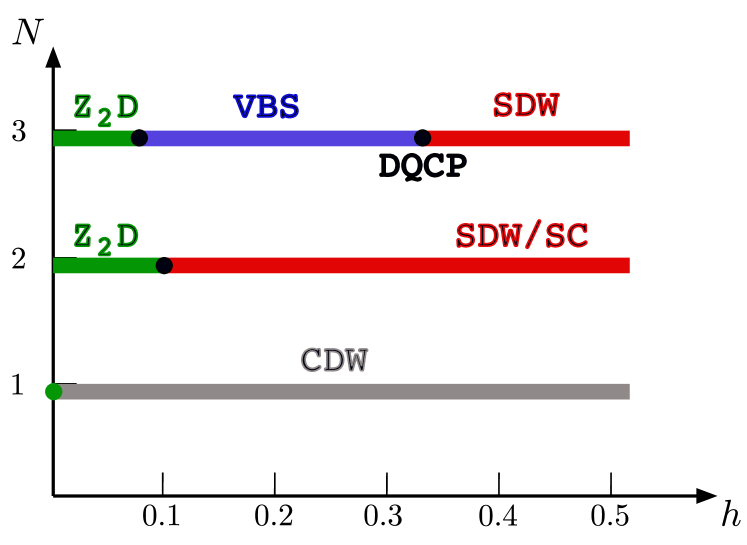
Figure 1: (color online) Schematic zero temperature phase diagram of the model in Eq. 1. We observe a $\mathbb{Z}_{2}$ Dirac deconfined phase ($Z_{2}$D), a spin-density wave (SDW) phase ($\equiv$ Néel phase) (or a superconductor (SC), depending on the pattern of particle-hole symmetry breaking), a charge density wave (CDW) phase as well as a valence bond solid (VBS). For $N=1$, we do not find evidence for a $Z_{2}$D phase beyond $h=0$ consistent with the arguments in the main text. The phase transitions from the $Z_{2}$D to SDW/SC ($N=2$) and VBS ($N=3$) are seemingly continuous. At $N=3$ we observe a deconfined quantum critical point (DCQP) between the VBS and SDW phases.

Our Hamiltonian (Eq.1) is partially motivated by a recent study of nematic instability of a Fermi surface Schattner et al. (2015) and velocity fluctuations in Dirac metals Xu et al. (2016). It consists of $N$ species of fermions on the vertices of a square lattice interacting with quantum Ising spins that live on the links of the same square lattice. However, in contrast to the Hamiltonian in Ref. Schattner et al. (2015), our Hamiltonian has a local $\mathbb{Z}_{2}$ invariance, which leads to $L_{x}L_{y}$ conserved operators on a $L_{x}\times L_{y}$ lattice. Furthermore, we restrict ourselves to half-filling and thus at low energies, instead of a Fermi surface, we either obtain either no fermions (e.g. a Mott insulator) or Fermi points. These differences completely alter the phase diagram of our model compared to Ref. Schattner et al. (2015).

The phase diagram for various values of $N$ is summarized in Fig.1. For $N>1$, we find that when the kinetic energy of the aforementioned Ising spins is small compared to the kinetic energy of the fermions, the ground state resembles deconfined phase of the $\mathbb{Z}_{2}$ gauge theory coupled to $2N$ Dirac fermions (the $N=1$ case is special in that the deconfined fermions are unstable to infinitesimal interactions). However, as we will discuss in detail, there is an important distinction between this phase and the deconfined phase of a conventional $\mathbb{Z}_{2}$ gauge matter theory (Ref. Kogut and Susskind (1975); Fradkin and Shenker (1979); Senthil and Fisher (2000)). Namely, the local $\mathbb{Z}_{2}$ invariance in our model is an actual symmetry of the Hamiltonian in contrast to the so-called ‘gauge symmetry’ in gauge-matter theories which just corresponds to redundancy in the description of the physical states. This is because we do not project the Hilbert space of our Hamiltonian to gauge invariant states, that is, we do not impose the Gauss’s law. Instead, in our model, the Gauss’s law in the ground state emerges due to spontaneous symmetry breaking as the locally conserved operators order in a certain definite pattern. One physical significance of this is that in contrast to regular $\mathbb{Z}_{2}$ gauge theory, in our model, equal space, unequal time non-gauge invariant correlation functions do not vanish identically. Further, there is a finite temperature Ising transition corresponding to the restoration of the aforementioned symmetry.

As the kinetic energy of the Ising degrees of freedom is increased, we find that the aforementioned gapless Dirac deconfined phase enters a symmetry broken confined phase. The nature of symmetry breaking depends on the value of $N$. For $N=1$ it corresponds to a charge density wave, while for $N=2$, due to an enlarged symmetry, the symmetry broken phase can correspond to a superconductor or a spin density wave, depending on the sign of infinitesimal symmetry breaking field. The $N=3$ case is even richer. We find that after exiting the deconfined phase, the model enters a valence bond solid (VBS) phase, and as the tuning parameter controlling the kinetic energy of Ising spins is tuned further, the valence-bond solid quantum melts and yields a anti-ferromagnet phase. The phase transition between the VBS and Néel phase, if second-order, will correspond to a deconfined quantum critical point Senthil et al. (2004), reported earlier in the context of quantum magnets Sandvik (2007); Lou et al. (2009). Our results are consistent with a second order transition.

II Model and symmetries

Our model reads:

$$\hat{H}=\sum_{\left<\boldsymbol{i},\boldsymbol{j}\right>}\hat{Z}_{\langle\boldsymbol{i},\boldsymbol{j}\rangle}\left(\sum_{\alpha=1}^{N}\hat{c}^{\dagger}_{\boldsymbol{i},\alpha}\hat{c}_{\boldsymbol{j},\alpha}+\text{H.c.}\right)+Nh\sum_{\left<\boldsymbol{i},\boldsymbol{j}\right>}\hat{X}_{\langle\boldsymbol{i},\boldsymbol{j}\rangle}$$ (1)

Here, $\hat{c}^{\dagger}_{\boldsymbol{i},\alpha}$ creates a fermion of flavor $\alpha$ in a Wannier state centered around lattice site $\boldsymbol{i}$ of a square lattice and the sum runs over bonds of nearest neighbors. Each bond, $\boldsymbol{b}=\langle\boldsymbol{i},\boldsymbol{j}\rangle$, accommodates a two level system spanned by the Hilbert space $|0\rangle_{\boldsymbol{b}}$ and $|1\rangle_{\boldsymbol{b}}$ and in this basis, $\hat{Z}_{\langle\boldsymbol{i},\boldsymbol{j}\rangle}$, and $\hat{X}_{\langle\boldsymbol{i},\boldsymbol{j}\rangle}$, corresponds to the Pauli spin matrices $\left(\begin{smallmatrix}1&0\\ 0&-1\end{smallmatrix}\right)$ and $\left(\begin{smallmatrix}0&1\\ 1&0\end{smallmatrix}\right)$ respectively. $h$ tunes the strength of the transverse field. Note that we have set the coefficient of the hopping term to unity so that all energy scales, including the size of $h$ and the temperature $T$, will be measured relative to the hopping term.

II.1 Discrete Symmetries

The model (Eq.1) leads to a number of symmetries. The particle-hole symmetry we consider is

$$\hat{P}_{\alpha}^{-1}\hat{c}^{\dagger}_{\boldsymbol{i},\beta}\hat{P}_{\alpha}=\delta_{\alpha,\beta}e^{i\boldsymbol{K}\cdot\boldsymbol{i}}\hat{c}_{\boldsymbol{i},\beta}+\left(1-\delta_{\alpha,\beta}\right)\hat{c}^{\dagger}_{\boldsymbol{i},\beta}$$ (2)

and it satisfies

$$\left[\hat{P}_{\alpha},\hat{H}\right]=0.$$ (3)

As an explicit operator, $\hat{P}_{\alpha}=\prod_{i}(c_{\boldsymbol{i},\alpha}e^{i\boldsymbol{K}\cdot\boldsymbol{i}/2}+\hat{c}^{\dagger}_{\boldsymbol{i},\alpha}e^{-i\boldsymbol{K}\cdot\boldsymbol{i}/2})$ where $\bm{K}=\left(\pi,\pi\right)$. Thus it is a fermionic (bosonic) operator if the total number of lattice sites is odd (even). As it will become clearer later in the paper, it is helpful to define a $\mathbb{Z}_{2}$ valued order-parameter $\hat{p}_{\boldsymbol{i}}$ that captures the breaking of the particle-hole symmetry,

$$\hat{p}_{\boldsymbol{i}}=\prod_{\alpha=1}^{N}\left(1-2\hat{n}_{\boldsymbol{i},\alpha}\right)=\left(-1\right)^{\hat{N}_{\boldsymbol{i}}}$$ (4)

This is nothing but the parity of fermion particle number at site $\boldsymbol{i}$. Under particle-hole transformation, $\hat{p}_{\boldsymbol{i}}\rightarrow-\hat{p}_{\boldsymbol{i}}$.

A more interesting symmetry corresponds to the local conservation laws:

$$\left[\hat{Q}_{\boldsymbol{i}},\hat{H}\right]=0$$ (5)

where

$$\hat{Q}_{\boldsymbol{i}}=\hat{X}_{\boldsymbol{i},\boldsymbol{i}+\boldsymbol{a}_{x}}\hat{X}_{\boldsymbol{i},\boldsymbol{i}-\boldsymbol{a}_{x}}\hat{X}_{\boldsymbol{i},\boldsymbol{i}+\boldsymbol{a}_{y}}\hat{X}_{\boldsymbol{i},\boldsymbol{i}-\boldsymbol{a}_{y}}\hat{p}_{\boldsymbol{i}}$$ (6)

with $\left[\hat{Q}_{\boldsymbol{i}},\hat{Q}_{\boldsymbol{j}}\right]=0$ and $\hat{Q}_{\boldsymbol{i}}^{2}=1$. Despite an extensive number of conservation laws, our Hamiltonian is not integrable. This is because the total number of degrees of freedom, $N_{dof}$, after taking into account $L_{x}L_{y}$ number of conserved $\hat{Q}_{\boldsymbol{i}}$’s on a $L_{x}\times L_{y}$ lattice, are still extensive: $N_{dof}=$ Number of Ising spins $+$ Number of fermions $-$ Number of constraints $=2L_{x}L_{y}+NL_{x}L_{y}-L_{x}L_{y}=(N+1)L_{x}L_{y}$.

Crucially, the operators $\hat{Q}_{\boldsymbol{i}}$ anti-commute with the generator of particle-hole symmetry: $\hat{P}^{-1}_{\alpha}\hat{Q}_{\boldsymbol{i}}\hat{P}_{\alpha}=-\hat{Q}_{\boldsymbol{i}}$. Therefore, the low energy theory of our model cannot contain terms that are proportional to $\hat{Q}_{\boldsymbol{i}}$ unless the particle-hole symmetry is spontaneously broken. The anti-commutation also implies that the energy eigenstates cannot simultaneously be particle-hole symmetric and eigenstates of $\hat{Q}_{\boldsymbol{i}}$. In particular, particle-hole symmetric eigenstates satisfy $\langle\hat{Q}_{\boldsymbol{i}}\rangle=0$. However, it’s worth emphasizing that even if an energy eigenstate is not particle-hole symmetric, it does not necessarily break the particle-hole symmetry spontaneously. For example, one can in principle construct a state $|\psi\rangle$ which is an eigenstate of all $\hat{Q}_{\boldsymbol{i}}$’s, (and therefore cannot be eigenstate of $\hat{P}_{\alpha}$ for any $\alpha$), but nevertheless satisfies $\langle\psi|\hat{p}_{\boldsymbol{i}}|\psi\rangle=0$, and $\langle\psi|\hat{p}_{\boldsymbol{i}}\hat{p}_{\boldsymbol{j}}|\psi\rangle\rightarrow 0$ as $|{\boldsymbol{i}}-{\boldsymbol{j}}|\rightarrow\infty$.

Another consequence of anticommutation between $\hat{Q}_{\boldsymbol{i}}$ and $\hat{P}_{\alpha}$ is that the spectra of the Hamiltonian is at least doubly degenerate. In fact, on a lattice with an odd number of total sites, the Hamiltonian possesses a $\mathcal{N}=2$ SUSY Hsieh et al. (2016). This is because, as discussed in $\hat{P}_{\alpha}$ is a fermionic operator and together with bosonic operator $\hat{Q}_{\boldsymbol{i}}$ can be used to define a fermionic SUSY generator $\mathcal{Q}=\sqrt{H/2}\hat{P}_{\alpha}(1+\hat{Q}_{\boldsymbol{i}})$ for any $\alpha$ and $\bm{i}$, so that $\{\mathcal{Q},\mathcal{Q}^{\dagger}\}=2H$, $\mathcal{Q}^{2}=0$, and $[\mathcal{Q},H]=0$.

At this point it is important to pause and note that even though our Hamiltonian (Eqn.1) bears a strong resemblance to a $\mathbb{Z}_{2}$ gauge theory coupled to matter fields Kogut and Susskind (1975); Fradkin and Shenker (1979); Senthil and Fisher (2000), ours is actually not a gauge theory due to an important difference. Unlike a matter-gauge theory, we do not impose the Gauss’s law constraint at any site. In a conventional $\mathbb{Z}_{2}$ gauge theory, the field $\hat{X}_{\boldsymbol{i},\boldsymbol{i}+\hat{n}}$ would correspond to the $\mathbb{Z}_{2}$ electric field along direction $\hat{n}$ at site $\boldsymbol{i}$, and thus the Gauss’s law (‘$\bm{\nabla}.\bm{E}=\rho$’) reads: $\hat{X}_{\boldsymbol{i},\boldsymbol{i}+\boldsymbol{a}_{x}}\hat{X}_{\boldsymbol{i},\boldsymbol{i}-\boldsymbol{a}_{x}}\hat{X}_{\boldsymbol{i},\boldsymbol{i}+\boldsymbol{a}_{y}}\hat{X}_{\boldsymbol{i},\boldsymbol{i}-\boldsymbol{a}_{y}}\,(\equiv\bm{\nabla}.\bm{E})=\hat{p}_{\boldsymbol{i}}\,(\equiv\rho)$. Satisfying this operator equation would thus require projecting the Hamiltonian to a specific set of eigenvalues of operators $\hat{Q}_{\boldsymbol{i}}$ (namely, $\hat{Q}_{\boldsymbol{i}}=1$ ). In contrast, we do not impose any constraint on $\hat{Q}_{\boldsymbol{i}}$’s, which therefore behave like classical degrees of freedom, whose values are allowed to vary from one eigenstate to another, and for a given many-body eigenstate these values will be determined by the intrinsic dynamics of our Hamiltonian.

The local conservation of $\hat{Q}_{\boldsymbol{i}}$ has important consequences. Since $\hat{Q}_{\boldsymbol{i}}\hat{c}^{\dagger}_{\boldsymbol{j},\alpha}{\hat{Q}_{\boldsymbol{i}}}^{-1}=\left(1-2\delta_{\boldsymbol{i},\boldsymbol{j}}\right)\hat{c}^{\dagger}_{\boldsymbol{j},\alpha}$, one can readily show that

$$\langle\hat{c}^{\dagger}_{{\boldsymbol{i}}_{1},\alpha}(\tau)\hat{c}_{{\boldsymbol{i}}_{n},\alpha}(0)\rangle=\delta_{\boldsymbol{i}_{1},\boldsymbol{i}_{n}}\langle\hat{c}^{\dagger}_{{\boldsymbol{i}}_{1},\alpha}(\tau)\hat{c}_{{\boldsymbol{i}}_{1},\alpha}(0)\rangle.$$ (7)

or equivalently

$$\langle\hat{Z}_{{\boldsymbol{b}}}(\tau)\hat{Z}_{{\boldsymbol{b}}^{\prime}}(0)\rangle=\delta_{\boldsymbol{b},\boldsymbol{b}^{\prime}}\langle\hat{Z}_{{\boldsymbol{b}}}(\tau)\hat{Z}_{{\boldsymbol{b}}}(0)\rangle.$$ (8)

Thus, a bare single fermion $\hat{c}_{\boldsymbol{i},\alpha}$ as well as the Ising operator $\hat{Z}$, are localized along the real space axis, but can propagate along the imaginary time direction. Propagation along the imaginary time implies transitions between different $\hat{Q}_{\boldsymbol{i}}$ sectors which is not prohibited in our model. As already mentioned, if one were to instead impose a constraint on the values of $\hat{Q}_{\boldsymbol{i}}$, it would prohibit propagation along the time direction as well, leading to a local $\mathbb{Z}_{2}$ gauge redundancy.

On the other hand, quantities such as

$$\langle\hat{c}^{\dagger}_{{\boldsymbol{i}}_{1},\alpha}(\tau)\prod_{j=1}^{n-1}\hat{Z}_{\langle\boldsymbol{i}_{j},\boldsymbol{i}_{j+1}\rangle}\left(\tau_{j}\right)\hat{c}_{\boldsymbol{i}_{n},\alpha}(0)\rangle$$ (9)

where one attaches a string of $\hat{Z}$-operators along certain chosen bonds connecting $\boldsymbol{i}_{1}$ to $\boldsymbol{i}_{n}$, as well as closed paths of $\hat{Z}$-operators, or the expectation value of $\hat{X}_{\langle\boldsymbol{i},\boldsymbol{j}\rangle}$ are all quantities which do not vanish due to symmetry arguments. Again, since the Hilbert space is not restricted to a single choice of $\hat{Q}_{i}$ the strings are continuous in space but can be discontinuous in the imaginary time.

II.2 Continuous Symmetries

The model is clearly invariant under global U($N$) rotations in flavor space:

$$\hat{c}^{\dagger}_{\boldsymbol{i},\alpha}\rightarrow\sum_{\beta=1}^{N}U_{\alpha,\beta}\hat{c}^{\dagger}_{\boldsymbol{i},\beta}$$ (10)

where $U$ corresponds to an U($N$) matrix. We recall that U($N$) = $\frac{\textrm{SU}(N)\times\textrm{U}(1)}{Z_{N}}$ where the SU($N$) component corresponds to the rotations among the $N$-flavors and the U(1) corresponds to the global particle number conservation $c_{\bm{i},\alpha}\rightarrow e^{i\theta}c_{\bm{i},\alpha}$.

In fact, the full set of continuous symmetries is bigger than U($N$) and corresponds to O(2$N$). This symmetry is manifest if one makes a unitary transformation $c_{\boldsymbol{j},\alpha}\rightarrow ic_{\boldsymbol{j},\alpha}$ on only one of the sublattices of the square lattice, and then writes the complex fermions in terms of their Majorana components: $c_{\boldsymbol{j},\alpha}=\left(\gamma_{\boldsymbol{j},\alpha,1}+i\gamma_{\boldsymbol{j},\alpha,2}\right)/2$. The Hamiltonian then becomes:

$$\hat{H}=\sum_{\left<\boldsymbol{i},\boldsymbol{j}\right>}\hat{Z}_{\langle\boldsymbol{i},\boldsymbol{j}\rangle}\left(\sum_{\alpha=1}^{N}\sum_{a=1,2}i\gamma_{\boldsymbol{i},\alpha,a}\gamma_{\boldsymbol{j},\alpha,a}\right)+Nh\sum_{\left<\boldsymbol{i},\boldsymbol{j}\right>}\hat{X}_{\langle\boldsymbol{i},\boldsymbol{j}\rangle}$$ (11)

which is manifestly O(2$N$) invariant.

Since we are in two spatial dimensions, the aforementioned global continuous symmetry can break spontaneously at zero temperature. In many of the examples we will discuss, the symmetry breaking will be manifest in long-ranged correlation functions such as:

$$S_{\text{Spin}}(\boldsymbol{i}-\boldsymbol{j},\tau-\tau^{\prime})=\frac{1}{N}\sum_{\alpha,\beta}\langle\hat{S}^{\alpha}_{\;\;\beta}(\boldsymbol{i},\tau)\hat{S}^{\beta}_{\;\;\alpha}(\boldsymbol{j},\tau^{\prime})\rangle.$$ (12)

Here

$$\hat{S}^{\alpha}_{\;\;\beta}(\boldsymbol{i})=\hat{c}^{\dagger}_{\boldsymbol{i},\alpha}\hat{c}_{\boldsymbol{i},\beta}-\frac{1}{N}\delta_{\alpha,\beta}\sum_{\gamma=1}^{N}\hat{c}^{\dagger}_{\boldsymbol{i},\gamma}\hat{c}_{\boldsymbol{i},\gamma}$$ (13)

are the generators of the subgroup SU(N) of the aforementioned O(2$N$) symmetry.

Before moving on, we note that the discrete particle-hole symmetry provides exact mapping between seemingly different correlations functions. For example, let us consider the transverse ($\alpha\neq\beta$) spin operator

$$\hat{P}^{-1}_{\beta}\hat{S}^{\alpha}_{\;\;\beta}(\boldsymbol{i},\tau)\hat{P}_{\beta}=e^{i\boldsymbol{K}\cdot\boldsymbol{i}}\hat{c}^{\dagger}_{\boldsymbol{i},\alpha}(\tau)\hat{c}^{\dagger}_{\boldsymbol{i},\beta}(\tau).$$ (14)

Hence, the particle-hole condensate at $\boldsymbol{q}=\boldsymbol{K}=\left(\pi,\pi\right)$ is equivalent to a particle-particle condensate at $\boldsymbol{q}=\left(0,0\right)$. Equivalently, a charge density wave at $\boldsymbol{q}=\left(\pi,\pi\right)$ transforms to a diagonal spin-density wave at the same wave vector.

III Effective model at weak and strong coupling

III.1 Strong transverse field limit

In this limit, we can understand the model in terms of a Su-Schrieffer-Heeger coupling Su et al. (1980) to an Einstein phonon mode of frequency $h$, but with a truncated phonon Hilbert space. This reading of the model is certainly valid in the high frequency limit where phonon modes are not highly occupied. In particular, and in the $|\pm\rangle=\frac{1}{\sqrt{2}}\left(|1\rangle+|0\rangle\right)$ basis, we can represent the Ising spins in terms of hard core bosons:

$$\hat{X}_{\boldsymbol{b}}=2\hat{b}^{\dagger}_{\boldsymbol{b}}\hat{b}_{\boldsymbol{b}}-1,\;\;\;\;\hat{Z}_{\boldsymbol{b}}=\hat{b}^{\dagger}_{\boldsymbol{b}}+\hat{b}_{\boldsymbol{b}}$$ (15)

At high frequencies, the occupation of the bosonic level will be small so that one can safely relax the hard-core boson constraint, $\left(\hat{b}^{\dagger}_{\boldsymbol{b}}\right)^{2}=0$, and promote the bosonic operators to soft core ones. In this approximation, the analogy to phonons is exact. Integrating out the phonons leads to a retarded interaction resulting in the action:

$$S=-\frac{1}{2Nh}\sum_{\langle\boldsymbol{i},\boldsymbol{j}\rangle}\int_{0}^{\beta}{\text{d}}\tau{\text{d}}\tau^{\prime}\hat{k}_{\langle\boldsymbol{i},\boldsymbol{j}\rangle}(\tau)D(\tau-\tau^{\prime})\hat{k}_{\langle\boldsymbol{i},\boldsymbol{j}\rangle}(\tau^{\prime})$$ (16)

with

$$\hat{k}_{\langle\boldsymbol{i},\boldsymbol{j}\rangle}=\sum_{\alpha=1}^{N}\left(\hat{c}^{\dagger}_{\boldsymbol{i},\alpha}\hat{c}_{\boldsymbol{j},\alpha}+\text{H.c.}\right),$$ (17)

the local hopping term, and

$$D(\tau)=h\frac{e^{-2\left(\beta-|\tau|\right)h}+e^{-2|\tau|h}}{1-e^{-2\beta h}},$$ (18)

the bosonic propagator for $-\beta<\tau<\beta$. In the high frequency limit and for constant values of $\beta$ the interaction becomes instantaneous $\lim_{h\rightarrow\infty}D(\tau)=\delta(\tau)$ and the full Hamiltonian reduces to

$$\hat{H}_{\infty}=-\frac{1}{2Nh}\sum_{\left<\boldsymbol{i},\boldsymbol{j}\right>}\hat{k}^{2}_{\langle\boldsymbol{i},\boldsymbol{j}\rangle}.$$ (19)

This interaction was recently considered in the context of SU($N$) fermions on the honeycomb lattice in Ref. Li et al. (2015).

The form in Eq. 19 is easy to understand. In the strong coupling limit, the Ising spins are polarized along the $x$-direction, and fermion hopping is prohibited since this implies flipping of the spin against the transverse field. Virtual processes can nevertheless occur and generate a super exchange energy scale $J\propto\frac{1}{2Nh}$ .

It is instructive to consider the nature of phases in this limit for a few values of $N$. First, at large $N$, the Hamiltonian $\hat{H}_{\infty}$ in Eq.19 can be solved exactly (Ref.Affleck and Marston (1988)) and the ground state corresponds to a valence bond solid state. For $N=1$ case, the Hamiltonian is simply $H=\frac{1}{2Nh}\sum_{\langle\boldsymbol{i},\boldsymbol{j}\rangle}\left(n_{\boldsymbol{i}}-\frac{1}{2}\right)\left(n_{\boldsymbol{j}}-\frac{1}{2}\right)$ and thus the ground state corresponds to a charge-density wave. For $N=2$ case, one finds

$$-\frac{1}{4h}\sum_{\left<\boldsymbol{i},\boldsymbol{j}\right>}\hat{k}^{2}_{\langle\boldsymbol{i},\boldsymbol{j}\rangle}=\frac{1}{h}\sum_{\left<\boldsymbol{i},\boldsymbol{j}\right>}\left(\hat{\boldsymbol{S}}_{\boldsymbol{i}}\hat{\boldsymbol{S}}_{\boldsymbol{j}}+\hat{\boldsymbol{\eta}}_{\boldsymbol{i}}\hat{\boldsymbol{\eta}}_{\boldsymbol{j}}\right).$$ (20)

Here $\hat{\boldsymbol{S}}_{\boldsymbol{i}}$ is the spin-1/2 operator and $\hat{\boldsymbol{\eta}}_{\boldsymbol{i}}=\hat{P}^{-1}_{\uparrow}\hat{\boldsymbol{S}}_{\boldsymbol{i}}\hat{P}_{\uparrow}$ is the ‘Anderson’s pseudospin’ Anderson (1958),. In the strong coupling limit charge is localized and the Ising spins are frozen in the $x$-direction wave functions. Such functions have well defined quantum numbers $\hat{Q}_{\boldsymbol{i}}$. If one choses $\hat{Q}_{\boldsymbol{i}}=-1$, then the ground state will be a Néel state for the fermions while the Ising spins point along the x-direction. It is interesting to note that at $h=\infty$ the kinetic energy vanishes and that all real space charge configurations and thereby all $\hat{Q}_{\boldsymbol{i}}$ sectors are degenerate.

III.2 Weak transverse field limit

In the $h\rightarrow 0$ limit, the imaginary time scale on which the Ising spins can fluctuate diverges such that the Ising spin degrees of freedom become classical. The model then reduces to

$$\hat{H}_{0}=\sum_{\left<\boldsymbol{i},\boldsymbol{j}\right>}Z_{\langle\boldsymbol{i},\boldsymbol{j}\rangle}\left(\sum_{\alpha=1}^{N}\hat{c}^{\dagger}_{\boldsymbol{i},\alpha}\hat{c}_{\boldsymbol{j},\alpha}+\text{H.c.}\right)$$ (21)

and one has to find an arrangement of Ising spins which will minimize the energy. Local $\mathbb{Z}_{2}$ invariance implies that the energy of an eigenstate depends only on the $\mathbb{Z}_{2}$ flux $\hat{F}_{\boldsymbol{i}}$ through a plaquette:

$$\hat{F}_{\boldsymbol{i}}= \hat{Z}_{\langle\boldsymbol{i},\boldsymbol{i}+\boldsymbol{a}_{x}\rangle}\hat{Z}_{\langle\boldsymbol{i}+\boldsymbol{a}_{x},\boldsymbol{i}+\boldsymbol{a}_{x}+\boldsymbol{a}_{y}\rangle}\times$$ (22)

$$\hat{Z}_{\langle\boldsymbol{i}+\boldsymbol{a}_{x}+\boldsymbol{a}_{y},\boldsymbol{i}+\boldsymbol{a}_{y}\rangle}\hat{Z}_{\langle\boldsymbol{i}+\boldsymbol{a}_{y},\boldsymbol{i}\rangle}.$$

Lieb’s work Lieb (1994) implies that the minimal energy is realized by $\pi$-flux configurations i.e. $\hat{F}_{\boldsymbol{i}}=-1$. This means that the coupling to the fermions effectively generates a $\mathbb{Z}_{2}$ magnetic field term

$$|J|\sum_{\boldsymbol{i}}\hat{F}_{\boldsymbol{i}}$$ (23)

in the Hamiltonian.

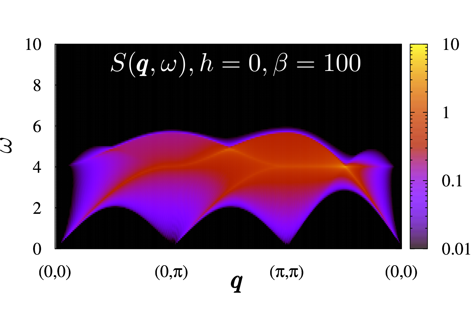
Figure 2: (color online) Dynamical spin structure factor at $h=0$. At the considered temperature we can safely neglect the thermal fluctuations of the Ising fields. Only Ising field configurations with a $\pi$-flux per plaquette contribute.

On the torus with $L_{x}\times L_{y}$ sites, there are $2^{L_{x}L_{y}}$ configurations of the Ising field that correspond to the $\pi$-flux through every plaquette, and therefore, an equal number of ground states at $h=0$. This huge ground state degeneracy can also be thought of as a result of the conserved quantities $\hat{Q}_{\boldsymbol{i}}$ that relate different ground states. To see the effect of $\pi$-flux on fermions, let us chose a two orbital unit cell with unit vectors $\boldsymbol{a}_{\pm}=\boldsymbol{a}_{x}\pm\boldsymbol{a}_{y}$ such that the intra-unit cell Ising field is $-1$ while all others are set to $1$. As mentioned above, the single particle spectral function depends on the specific choice of Ising fields. On the other hand, the two particle Green functions in the particle-hole channel are independent of the background Ising configuration. In Fig. 2, we plot the ground state dynamical spin-spin correlations function, $S(\boldsymbol{q},\omega)$, valid for all $N$. One observes a particle-hole continuum with gapless excitations at wave vectors connecting the Dirac cones $\boldsymbol{q}=(\pi,0)$ and $\boldsymbol{q}=(\pi,\pi)$. One key interest of the QMC simulations will be to study the fate of this particle-hole continuum at non-zero values of $h$.

As one might expect, and in accord with the third law of thermodynamics, quantum fluctuations will lift the zero temperature finite entropy density. In general, at non-zero values of $h$ terms which do not violate symmetries of the model will be dynamically generated. In particular, alongside the magnetic field term of Eq. 23 one can write down,

$$\hat{H}_{Q}=\sum_{\boldsymbol{i},\boldsymbol{j}}K_{\boldsymbol{i},\boldsymbol{j}}\hat{Q}_{\boldsymbol{i}}\hat{Q}_{\boldsymbol{j}}.$$ (24)

which is invariant under the particle-hole symmetry that sends $\hat{Q}_{\boldsymbol{i}}\rightarrow-\hat{Q}_{\boldsymbol{i}}$. Since this is nothing but a classical Ising Hamiltonian, one can foresee that there will likely be a finite temperature Ising transition below which the $\hat{Q}_{\boldsymbol{i}}$’s spontaneously order. As discussed in the following sections, this symmetry breaking will result in an emergent $\mathbb{Z}_{2}$ gauge structure in the ground state phase diagram and would also determine the nature of both confined and deconfined phases.

IV Methodology

In the Majorana representation of Eq. 11 the O(2$N$) symmetry of our model is manifest. As a consequence, sign free quantum Monte Carlo (QMC) simulations can be carried out for all values of $N$ Li et al. (2015). We have used a standard implementation of the finite temperature auxiliary field approach Hirsch et al. (1982); Blankenbecler et al. (1981); Assaad and Evertz (2008) to evaluate

$$\langle\hat{O}\rangle=\frac{\text{Tr}\left[e^{-\beta\hat{H}}\hat{O}\right]}{\text{Tr}\left[e^{-\beta\hat{H}}\right]}$$ (25)

where the trace runs over the fermionic and Ising degrees of freedom and $\beta$ corresponds to the inverse temperature. For Hubbard type model simulations, the auxiliary field corresponds to a Hubbard-Stratonovitch field with no explicit imaginary time dynamics Hirsch et al. (1982); Blankenbecler et al. (1981); Assaad and Evertz (2008). Here, in contrast, the auxiliary field corresponds to the z-component of the Ising field, and its imaginary time dynamics is controlled by the transverse field. We have adopted a single spin flip algorithm, which turns out to be efficient (high acceptance rates) at large values of $h$ where the field oscillates rapidly in imaginary time. At weak couplings, the Ising field becomes classical and the single spin-flip update in space-time becomes increasingly inefficient. This renders simulations at low values of $h$ expensive. Unless mentioned otherwise we have used a Trotter time step $\Delta\tau=0.2$ so as to allow for a bond decomposition of the infinitesimal time propagator: $e^{-\Delta\tau\hat{H}}\simeq\prod_{\boldsymbol{b}}e^{-\Delta\tau\hat{H}_{\boldsymbol{b}}}$, where $\hat{H}_{\boldsymbol{b}}$ corresponds to the Hamiltonian on a single bond. Within the auxiliary field QMC method one can compute equal time as well as imaginary time displaced correlation functions. We have carried out the analytical continuation with a stochastic implementation of the Maximum Entropy method Sandvik (1998); Beach (2004). Eq. 7, which states that the single-particle Green’s function is independent of momentum, provides an ideal test for the QMC as well as for the analytical continuation since the locality of the single particle Green function results from the Monte Carlo sampling. Fig. 3 shows the single particle spectral function $A(\boldsymbol{k},\omega)=-\text{Im }G^{\text{ret}}(\boldsymbol{k},\omega)$ for $N=1$ model which is obtained from Wick rotation of the imaginary time Green function $G(\boldsymbol{k},\tau)=-\langle T\hat{c}_{\boldsymbol{k}}(\tau)\hat{c}_{\boldsymbol{k}}^{\dagger}(0)\rangle$. The $\boldsymbol{k}$-independence of the data should be seen as a measure of our spectral resolution.

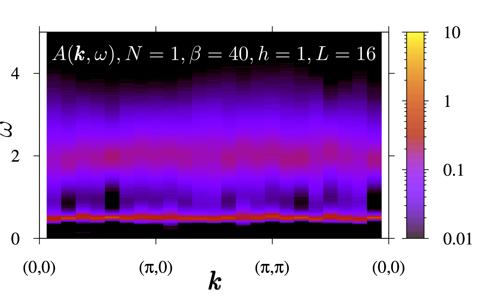
Figure 3: (color online) Single-particle spectral function $A(\boldsymbol{k},\omega)$ for the $N=1$ model. As argued in the text, $A(\boldsymbol{k},\omega)$ is $\boldsymbol{k}$-independent.

V Numerical results

In this section we will describe our numerical results obtained from finite temperature auxiliary field simulations.

Summary of Results

A sketch of the zero temperature phase diagram in the transverse field $h$ versus $N$ plane is shown in Fig. 1. We will argue below that for all values of $N$, there is a finite temperature Ising transition at which the $\hat{Q}_{\boldsymbol{i}}$ operators order. Since $\left[\hat{Q}_{\boldsymbol{i}},\hat{H}\right]=0$, this is akin to spontaneous symmetry breaking in a classical Ising model. For even (odd) values of $N$ we observe (anti) ferromagnetic ordering of the $\hat{Q}_{\boldsymbol{i}}$’s so that at zero temperature we can understand our results in terms of an effective $\mathbb{Z}_{2}$ gauge theory coupled to 2$N$ Dirac fermions, with the understanding that non-gauge invariant unequal time, equal-space correlators do not vanish, as discussed earlier. The (anti) ferromagnetic ordering for even (odd) values of $N$ is consistent with the fact that perturbatively, the couplings $K_{i,j}$ in Eq. 24 for nearest neighbour vertices are proportional to $(-1)^{N+1}$.

Spontaneous breaking of $\hat{Q}_{\boldsymbol{i}}\rightarrow-\hat{Q}_{\boldsymbol{i}}$ generates term proportional to $\sum_{i}e^{iN\boldsymbol{K}\cdot\boldsymbol{i}}\hat{p}_{\boldsymbol{i}}$ in the effective Hamiltonian, leading to spontaneous charge ordering of fermions below the finite temperature transition. The relevance/irrelevance of this term determines the fate of $h=0$ gapless Dirac fermions (Fig. 2) at infinitesimal $h$. When $N=1$, this term is a fermion bilinear proportional to $\sum_{i}e^{i\boldsymbol{K}\cdot\boldsymbol{i}}\left(1-2\hat{n}_{\boldsymbol{i}}\right)$ and thus leads to spontaneous charge-ordering and mass gap for fermions at infinitesimal $h$. For $N=2$, this term is proportional to the Hubbard term $\sum_{i}\left(1-2\hat{n}_{\boldsymbol{i},1}\right)\left(1-2\hat{n}_{\boldsymbol{i},2}\right)$ where the overall sign of this term is determined by whether $\langle\hat{Q}_{\boldsymbol{i}}\rangle=1$ or $-1$. The Hubbard term is irrelevant for gapless Dirac fermions, and therefore one expects to find a stable $\mathbb{Z}_{2}$ Dirac deconfined phase (Z₂D in Fig.1). Similarly, when $N=3$, the corresponding term $\sum_{i}e^{i\boldsymbol{K}\cdot\boldsymbol{i}}\left(1-2\hat{n}_{\boldsymbol{i},1}\right)\left(1-2\hat{n}_{\boldsymbol{i},2}\right)\left(1-2\hat{n}_{\boldsymbol{i},3}\right)$ is irrelevant at the $h=0$ point, leading again to a stable Z₂D phase.

As $h$ is increased, the aforementioned Dirac deconfined phase undergoes a transition to a symmetry broken confined phase whose nature depends on the value of $N$ (Fig.1). For $N=2$, we find a Néel antiferromagnet, or a superconductor depending on whether $\langle\hat{Q}_{\boldsymbol{i}}\rangle=-1$ or $1$, respectively. For $N=3$, we find two symmetry broken phases, a dimerized ($\equiv$ Valence Bond Solid) phase separated from the Z₂D phase again by a seemingly continuous transition, and a Néel phase at larger values of $h$. The transition between the spin-dimerized state and the Néel phase is apparently also continuous and thus provides an example of deconfined quantum critical point Senthil et al. (2004).

V.1 N=1

As already discussed briefly in Sec.II, in the large-$h$ limit, our model Hamiltonian (Eq.1) maps onto (Eq. 19)

$$\hat{H}_{\infty}=\frac{1}{h}\sum_{\left<\boldsymbol{i},\boldsymbol{j}\right>}\left(\hat{n}_{\boldsymbol{i}}-1/2\right)\left(\hat{n}_{\boldsymbol{j}}-1/2\right)$$ (26)

so that the ground state is a charge density wave. In this limit $\langle\hat{X}_{\boldsymbol{b}}\rangle\simeq 1$ and the charge ordering follows a $\boldsymbol{K}=(\pi,\pi)$ modulation. Consequently the $\hat{Q}_{\boldsymbol{i}}$’s, by definition (Eq.6), order anti-ferromagnetically. Therefore, as a function of temperature, there must be a finite temperature transition in the 2D Ising universality class below which the $\hat{Q}_{\boldsymbol{i}}$ develop long range order. In the absence of a particle-hole symmetry breaking field, $\langle\hat{Q}_{\boldsymbol{i}}\rangle=0$ on any finite lattice and one has to measure correlation functions to detect ordering. The $\langle\hat{Q}_{\boldsymbol{i}}\hat{Q}_{\boldsymbol{j}}\rangle$ correlation functions turn out to be very noisy and we have found it more convenient to include a small symmetry breaking field:

$$\hat{H}_{s}=h_{s}\sum_{\boldsymbol{i}}e^{i\boldsymbol{K}\cdot\boldsymbol{i}}\left(\hat{n}_{\boldsymbol{i}}-1/2\right).$$ (27)

Such a term in Hamiltonian does not introduce a negative sign problem Li et al. (2016) and pins the CDW. Since $\left[\hat{Q}_{\boldsymbol{i}},\hat{H}_{s}\right]=0$, $\hat{Q}_{\boldsymbol{i}}$ remains a good quantum number at finite value of $h_{s}$. In fact $\hat{H}_{s}$ acts on the Ising model of the $\hat{Q}_{\boldsymbol{i}}$ variables as a staggered magnetic field.

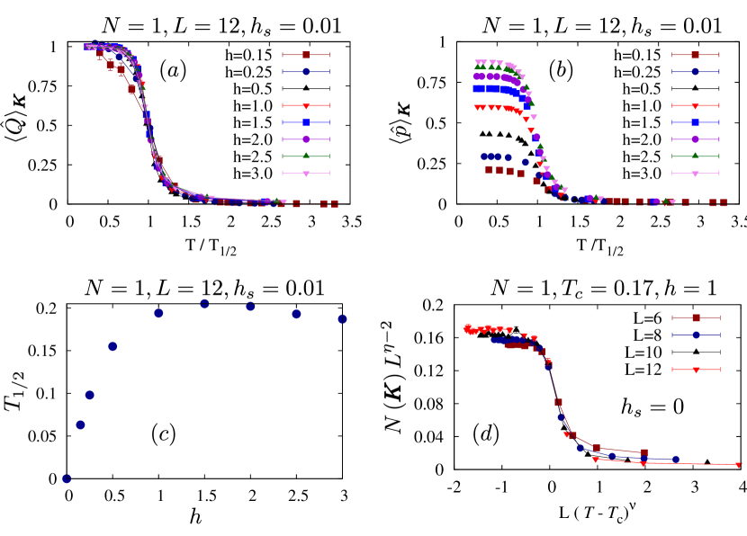
Figure 4: (color online) (a) Staggered order parameter of Eq. 28 at finite symmetry breaking field $h_{s}=0.01$. (b) Staggered order parameter of Eq. 31 again at finite symmetry breaking field $h_{s}=0.01$. The temperature scale is normalized by $T_{1/2}$ defined in Eq. 30. (c) $T_{1/2}$ as a function of $h$. (d) Data collapse of the density-density correlation function defined in Eq. 32. This correlation function is related to the CDW order parameter via Eq. 34. A reasonable data collapse is obtained using the 2D Ising exponents.

Figure 4(a) plots

$$\langle\hat{Q}\rangle_{\boldsymbol{K}}=\frac{1}{L^{2}}\sum_{\boldsymbol{i}=1}^{L^{2}}e^{i\boldsymbol{K}\cdot\boldsymbol{i}}\langle\hat{Q}_{\boldsymbol{i}}\rangle$$ (28)

at a small value of the particle-hole symmetry breaking field, $h_{s}=0.01$. At low temperatures we find that $\langle\hat{Q}\rangle_{\boldsymbol{K}}$ scales to unity for all values of $h$. Since $\hat{Q}_{\boldsymbol{i}}$ is a good quantum number, even in the presence of the symmetry breaking field, this means that the ground state has

$$\hat{Q}_{\boldsymbol{i}}=e^{i\boldsymbol{K}\cdot\boldsymbol{i}}$$ (29)

and the gauge constraint is dynamically generated. The temperature scale at which $\langle\hat{Q}\rangle_{\boldsymbol{K}}$ takes half of its maximal value defines $T_{1/2}$

$$\langle\hat{Q}\rangle_{\boldsymbol{K}}(T=T_{1/2})=1/2.$$ (30)

Figure 4(c) plots $T_{1/2}$ as a function of $h$. The plot is consistent with the expectation that $T_{1/2}$ vanishes at $h=0$ and $h=\infty$ since in both limits all $\hat{Q}_{\boldsymbol{i}}$ configurations are degenerate.

Ordering of $\hat{Q}_{\boldsymbol{i}}$ implies charge ordering. This is because the low-energy effective Hamiltonian now contains a term proportional to $\sum_{\boldsymbol{i}}e^{i\boldsymbol{K}\cdot\boldsymbol{i}}\hat{Q}_{\boldsymbol{i}}=\sum_{\boldsymbol{i}}e^{i\boldsymbol{K}\cdot\boldsymbol{i}}\hat{X}_{\boldsymbol{i},\boldsymbol{i}+\boldsymbol{a}_{x}}\hat{X}_{\boldsymbol{i},\boldsymbol{i}-\boldsymbol{a}_{x}}\hat{X}_{\boldsymbol{i},\boldsymbol{i}+\boldsymbol{a}_{y}}\hat{X}_{\boldsymbol{i},\boldsymbol{i}-\boldsymbol{a}_{y}}\hat{p}_{\boldsymbol{i}}$. At the same time, by symmetry, the effective Hamiltonian already contains a term proportional to $\sum_{\boldsymbol{i}}\hat{X}_{\boldsymbol{i},\boldsymbol{i}+\boldsymbol{a}_{x}}\hat{X}_{\boldsymbol{i},\boldsymbol{i}-\boldsymbol{a}_{x}}\hat{X}_{\boldsymbol{i},\boldsymbol{i}+\boldsymbol{a}_{y}}\hat{X}_{\boldsymbol{i},\boldsymbol{i}-\boldsymbol{a}_{y}}$. The product of these two terms, which will also be generated, is proportional to $\sum_{\boldsymbol{i}}e^{i\boldsymbol{K}\cdot\boldsymbol{i}}\hat{p}_{\boldsymbol{i}}$ and leads to charge-ordering. To confirm this, we have hence computed

$$\langle\hat{p}\rangle_{\boldsymbol{K}}=\frac{1}{L^{2}}\sum_{\boldsymbol{i}=1}^{L^{2}}e^{i\boldsymbol{K}\cdot\boldsymbol{i}}\langle\hat{p}_{\boldsymbol{i}}\rangle.$$ (31)

As apparent from Fig. 4(b) the energy scale at which $\langle\hat{p}\rangle_{\boldsymbol{K}}$ picks up, matches $T_{1/2}$ defined in Eq.30. As a further test we have computed charge-charge correlation functions in the absence of symmetry breaking field:

$$N(\boldsymbol{q})=\frac{1}{4}\sum_{\boldsymbol{r}}e^{i\boldsymbol{q}\cdot\boldsymbol{r}}\langle\hat{p}_{\boldsymbol{r}}\hat{p}_{\boldsymbol{0}}\rangle$$ (32)

where $\hat{p}_{\boldsymbol{i}}=\left(1-2\hat{n}_{\boldsymbol{i}}\right)$. At low temperatures, ordering occurs at the antiferromagnetic wave vector $\boldsymbol{K}=(\pi,\pi)$ and as shown in Fig. 4(c) a reasonable data collapse is obtained using the 2D Ising exponents, $\eta=1/4$ and $\nu=1$. For the value of $h=1$ considered in Fig. 4(d) we obtain $T_{c}\simeq 0.17$ which stands, to a first approximation, in agreement with the value of $T_{1/2}$ listed in Fig. 4(b).

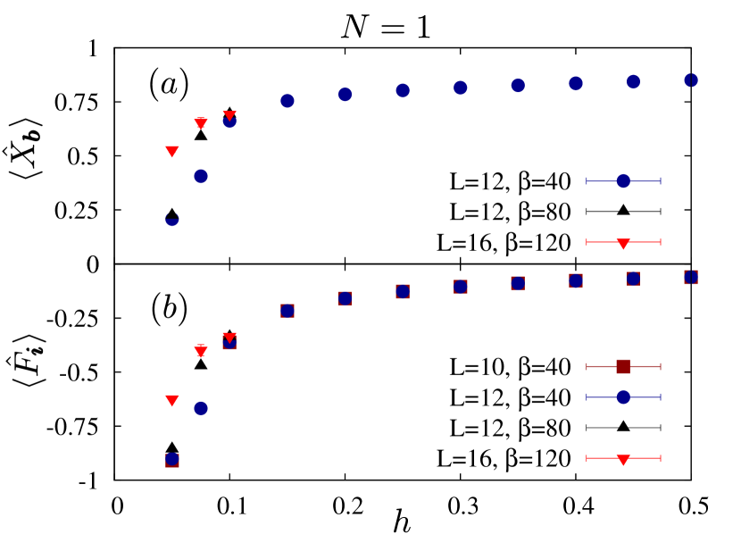
Figure 5: (color online) (a) Electric field and (b) magnetic flux for the $N=1$ model as a function of the transverse field. After taking into account the strong finite temperature and size effects in the small $h$ limit, the data is consistent with a smooth behavior.

Fig. 5 plots ‘gauge invariant’ quantities $\langle\hat{X}_{\boldsymbol{b}}\rangle$ and $\langle\hat{F}_{\boldsymbol{i}}\rangle$ (Eq.22) corresponding to the Ising field. We note that the average electric field is given by

$$\langle\hat{X}_{\boldsymbol{b}}\rangle=\frac{1}{L^{2}}\frac{\partial F}{\partial h}$$ (33)

where $F$ is the free energy, and therefore provides a direct access to the behavior of free energy as a function of $h$. At small values of $h$ one observes strong finite size and temperature effects for both quantities. Our lowest temperature results support a smooth crossover from $\langle\hat{X}_{\boldsymbol{b}}\rangle=0$, $\langle\hat{F}_{\boldsymbol{i}}\rangle=-1$ to $\langle\hat{X}_{\boldsymbol{b}}\rangle=1$, $\langle\hat{F}_{\boldsymbol{i}}\rangle=0$ as $h$ grows. This implies that there is no level crossing associated with a change of ground state quantum numbers and that the gauge constraint remains enforced for all values of the transverse field. At $h=0$ all plaquettes are threaded by a $\pi$-flux static magnetic field and no electric field is present. Starting form this limit gauge fluctuations introduce pairs of $\mathbb{Z}_{2}$ vortices – which are nothing but plaquettes with zero flux – such that as a function of $h$ the magnetic field grows. The fluctuations of the magnetic field induce the onset of the electric field.

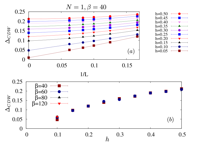
Figure 6: (color online) (a) Size extrapolation of the charge density wavve order parameter $\Delta_{CDW}$ performed with a second order polynomial in $1/L$. (b) Extrapolated value of $\Delta_{CDW}$ at different temperatures. Below $h=0.1$ our lattice sizes are too small to unambiguously extrapolate to the thermodynamic limit.

We now discuss zero-temperature phase diagram. The CDW order parameter,

$$\Delta_{CDW}=\sqrt{N(\boldsymbol{K})/L^{2}},$$ (34)

at low temperatures and as a function of $h$ is plotted in Fig. 6. Consistent with the fact that at $h=0$, the spectrum is gapless (Fig. 2), and correspondingly $T_{1/2}\rightarrow 0$ as $h\rightarrow 0$ (Fig. 4), the CDW order parameter also approaches zero as $h\rightarrow 0$. We expect that $\langle\hat{Q}_{\boldsymbol{i}}\rangle\neq 0$ for any non-zero $h$, and therefore the Z₂D phase is stable only at $h=0$.

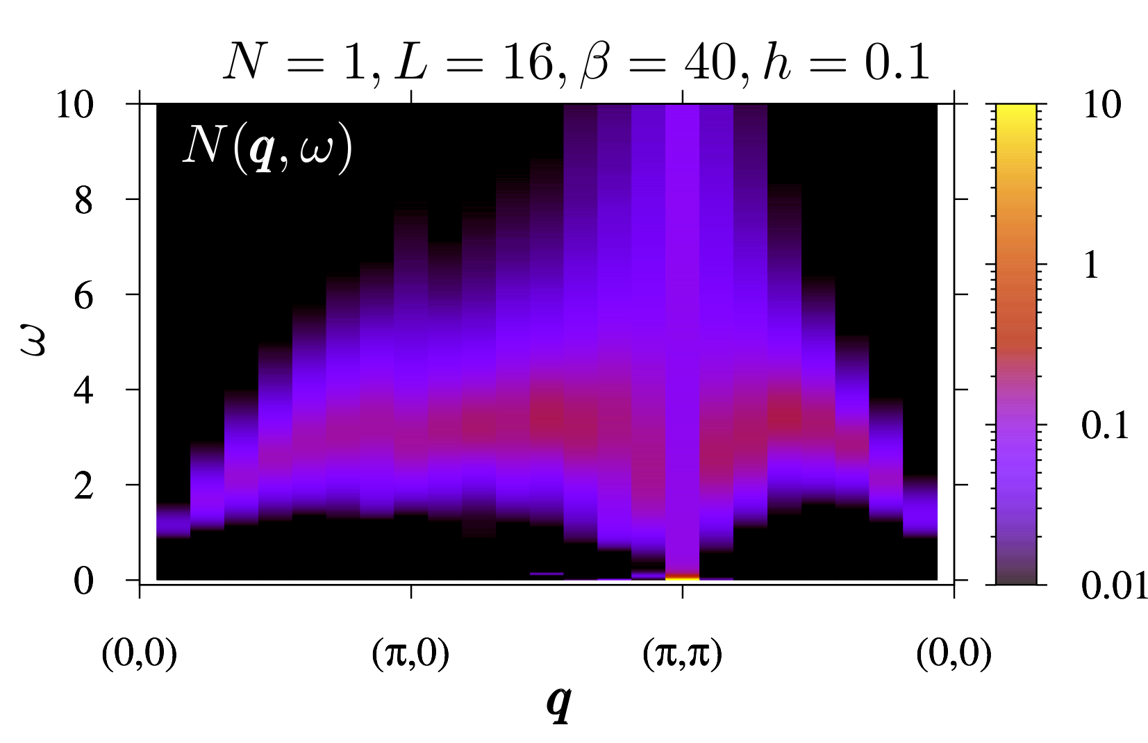
Figure 7: (color online) Dynamical charge structure factor for the $N=1$ model.

In Fig. 7 we consider the dynamical properties of the model at $h=0.1$ and $\beta=40$. This choice of parameters places us below $T_{1/2}$ and we will discuss the data in terms of the ground state with quantum numbers

$$\hat{Q}_{\boldsymbol{i}}|\Psi_{0}\rangle=e^{i\boldsymbol{K}\cdot\boldsymbol{i}}|\Psi_{0}\rangle.$$ (35)

The dynamical charge structure factor reads,

$$N(\boldsymbol{q},\omega)=\pi\sum_{n}|\langle\Psi_{n}|\hat{N}_{\boldsymbol{q}}|\Psi_{0}\rangle|^{2}\delta(E^{N}_{n}-E^{N}_{0}-\omega)$$ (36)

with

$$\hat{N}(\boldsymbol{q})=\frac{1}{L}\sum_{\boldsymbol{i}}e^{i\boldsymbol{q}\cdot\boldsymbol{i}}\hat{n}_{\boldsymbol{i}}.$$ (37)

The intermediate states, $|\Psi_{n}\rangle$, have the same $\hat{Q}_{\boldsymbol{i}}$ quantum numbers as in the ground state since $\left[\hat{n}_{\boldsymbol{i}},\hat{Q}_{\boldsymbol{i}}\right]=0$. Thereby, the dynamical charge structure factor of Fig. 7 is identical to that one would obtain when imposing exactly the gauge constraint on the Hilbert space. Within this constrained Hilbert space, the elementary excitations are closed Wilson loops of $\hat{Z}_{\boldsymbol{b}}$ operators in Euclidian space-time as well as open strings of $\hat{Z}_{\boldsymbol{b}}$ operators with particle-hole excitations at the extremities again in $2+1$ dimensions. For the considered values of $h$ the ground state shows long range CDW order and the gauge string binds particle-hole excitations. This corresponds to the confined phase of the gauge field and leads to the central peak feature at the wave vector $\boldsymbol{K}=(\pi,\pi)$ apparent in Fig. 7. In the limit $h\rightarrow\infty$ this becomes the dominant feature of the spectral function. At higher energies or on shorter time scales, the string does not bind particle-hole excitations and a continuum very reminiscent of the $h=0$ limit is apparent in the spectral function.

V.2 N=2

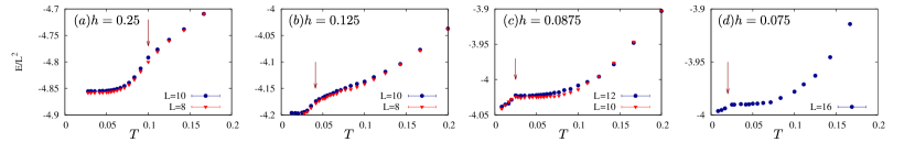
Figure 8: (color online) Energy as a function of temperature for the $N=2$ model at various values of $h$.

As discussed in the Sec.II.2, for $N=2$ the global symmetry is O(4). To understand the physical content of this symmetry, it is instructive to consider the limit $h\rightarrow\infty$:

$$\hat{H}_{\infty}= -\frac{1}{4h}\sum_{\left<\boldsymbol{i},\boldsymbol{j}\right>}\left[\sum_{\sigma=1}^{2}\left(\hat{c}^{\dagger}_{\boldsymbol{i},\sigma}\hat{c}_{\boldsymbol{j},\sigma}+\text{H.c.}\right)\right]^{2}$$

$$= \frac{1}{h}\sum_{\left<\boldsymbol{i},\boldsymbol{j}\right>}\left[\hat{\boldsymbol{S}}_{\boldsymbol{i}}\hat{\boldsymbol{S}}_{\boldsymbol{j}}+\hat{\boldsymbol{\eta}}_{\boldsymbol{i}}\hat{\boldsymbol{\eta}}_{\boldsymbol{j}}\right].$$ (38)

Here, $\hat{\boldsymbol{S}}_{\boldsymbol{i}}=\frac{1}{2}\sum_{\sigma,\sigma^{\prime}}\hat{c}^{\dagger}_{\boldsymbol{i},\sigma}\boldsymbol{\sigma}_{\sigma,\sigma^{\prime}}\hat{c}_{\boldsymbol{i},\sigma^{\prime}}$ corresponds to a fermionic representation of the spin operator and $\hat{\boldsymbol{\eta}}_{\boldsymbol{i}}=\hat{P}^{-1}_{1}\hat{\boldsymbol{S}}_{\boldsymbol{i}}\hat{P}_{1}$ where $\hat{P}_{1}$ corresponds to particle-hole symmetry transformation defined in Eq. 2. Since the $\boldsymbol{\eta}$-operators are derived from the spin operators with a similarity transformation they satisfy the SU(2) algebra as well. Furthermore, $\left[\hat{\eta}_{\boldsymbol{j},\alpha},\hat{S}_{\boldsymbol{i},\beta}\right]=0$ so that at the level of Lie algebra, the O(4) symmetry can be understood as O(4) $\cong$ SU${}_{S}(2)$ $\otimes$ SU${}_{\eta}(2)$ Yang and Zhang (1990), .

The Ising order parameter corresponding to particle-hole symmetry breaking (Eq. 4) relates to the $\hat{\boldsymbol{S}}$- and $\hat{\boldsymbol{\eta}}$-operators via

$$\hat{p}_{\boldsymbol{i}}=\frac{4}{3}\left(\hat{\boldsymbol{\eta}}_{\boldsymbol{i}}^{2}-\hat{\boldsymbol{S}}_{\boldsymbol{i}}^{2}\right).$$ (39)

If particle-hole symmetry breaks, then there are two possibilities. If $\langle\hat{p}_{\boldsymbol{i}}\rangle<0$, then the SU${}_{S}(2)$ $\otimes$ SU${}_{\eta}(2)$ is reduced to SU${}_{S}(2)$. In the extreme limit of $p=-1$, sites are singly occupied, and the model reduces to a spin-only model. Away from this limit, there are charge fluctuations per site, but the universal properties (such as the phase transition out of the deconfined phase), which depends only on symmetries, can still be understood in terms of only spin fluctuations. The other possibility is that $\langle\hat{p}_{\boldsymbol{i}}\rangle>0$, in which case the sites are predominantly empty or doubly occupied, leading to a charge-only model in the extreme limit $p=1$. In this case, the underlying symmetry is SU${}_{\eta}(2)$ and the phase diagram can be understood in terms of fluctuations of a three component vector consisting of CDW (one component) and s-wave superconductor ( two components, since it has both real and imaginary components). Since the superconducting phase, whenever it exists, is always degenerate with CDW due to SU${}_{\eta}(2)$ symmetry, henceforth we will call the corresponding phase as just superconductor.

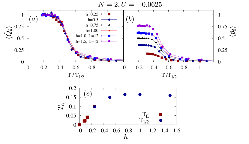
Figure 9: (color online) (a) Average value of $\langle\hat{Q}_{\boldsymbol{i}}\rangle$ in the presence of a small symmetry breaking field, $U=-0.0625$. (b) Average value of $\langle\hat{p}_{\boldsymbol{i}}\rangle$ at the same value of the symmetry breaking field. Unless mentioned otherwise, we have set $L=8$. (c) Estimate of $T_{c}$ below which we expect $\langle\hat{Q}_{\boldsymbol{i}}\rangle$ to order ferromagnetically. $T_{E}$ stems from the energy data of Fig. 8 and the temperature scale $T_{1/2}$ is defined by $\langle\hat{Q}_{\boldsymbol{i}}\rangle(T_{1/2})=1/2$.

To detect the possibility of Ising transitions corresponding to ordering of $\hat{Q}_{\boldsymbol{i}}$ and $\hat{p}_{\boldsymbol{i}}$ we compute the temperature dependence of the internal energy for a range of values of $h$ (Fig. 8). Note that in contrast to the $\hat{Q}_{\boldsymbol{i}}$’s, $\hat{p}_{\boldsymbol{i}}$ is not a good quantum number since $\left[\hat{p}_{\boldsymbol{i}},\hat{H}\right]\neq 0$. The Ising transition in two-dimensions has a specific heat exponent $\alpha=0$ which implies that the specific heat is logarithmic divergent at the transition temperature. This results in an infinite slope of the internal energy at $T_{c}$ and in the thermodynamic limit. An arrow in each plot points to the temperature where singularities are apparent. It is beyond the scope of our calculations to pin down the details of the singularity. In particular, when $T_{c}$ is small very large systems sizes are required to resolve the two dimensional nature of the singularity. Within our resolution we observe only one transition which we will now argue corresponds to the ordering of the $\hat{Q}_{\boldsymbol{i}}$’s as well as $\hat{p}_{\boldsymbol{i}}$, that is, breaking of particle-hole symmetry.

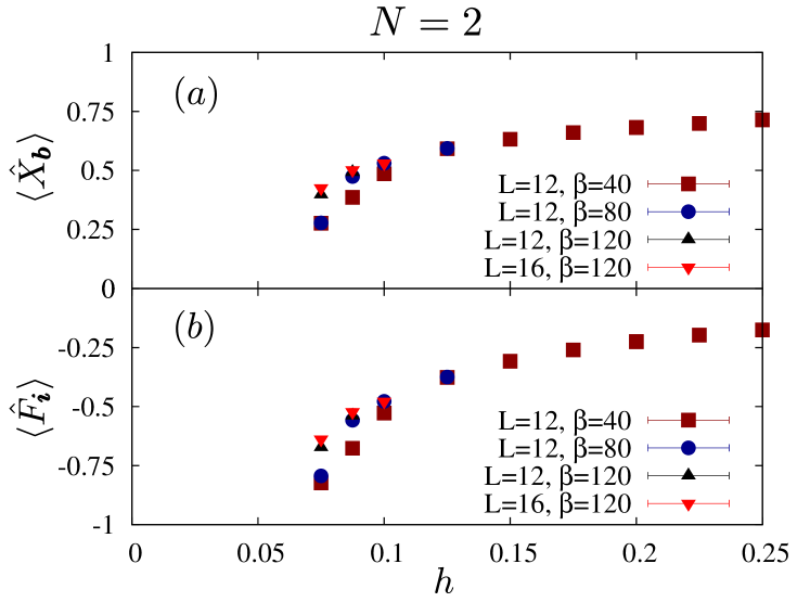
Figure 10: (color online) (a) Electric field and (b) magnetic flux per plaquette as a function of $h$ for the $N=2$ model.

To explicitly see the ordering of $\hat{Q}_{\boldsymbol{i}}$ and $\hat{p}_{\boldsymbol{i}}$, we add a small attractive Hubbard term to the model, $\hat{H}_{U}=-U\sum_{\boldsymbol{i}}\left(\hat{n}_{\boldsymbol{i},1}-1/2\right)\left(\hat{n}_{\boldsymbol{i},2}-1/2\right)$. This does not introduce a sign problem Wu and Zhang (2005), but breaks particle-hole symmetry and effectively acts as a uniform magnetic field for the $\hat{Q}_{\boldsymbol{i}}$ variables, alongside the Ising interaction term of Eq. 24. Note that $\left[\hat{H}_{U},\hat{Q}_{\boldsymbol{i}}\right]=0$ so that $\hat{Q}_{\boldsymbol{i}}$ remains a good quantum number upon inclusion of this symmetry breaking term. Fig. 9 shows $\langle\hat{Q}_{\boldsymbol{i}}\rangle$ as a function of temperature at small values of the Hubbard $U$. At an energy scale set by $T_{c}$ one observes a growth in $\langle\hat{Q}_{\boldsymbol{i}}\rangle$ which saturates to the value $\langle\hat{Q}_{\boldsymbol{i}}\rangle\simeq 1$. The fact that $\langle\hat{Q}_{\boldsymbol{i}}\rangle\simeq 1$ at low temperature implies ferromagnetic coupling between the $\hat{Q}_{\boldsymbol{i}}$ variables in Eq. 24. Since the Hubbard term acts as a Zeeman field for particle-hole symmetry as well, we can compute $\langle\hat{p}_{\boldsymbol{i}}\rangle$ to check if particle-hole symmetry is broken spontaneously at the same energy scale. If so, one expects $\langle\hat{p}_{\boldsymbol{i}}\rangle$ to show a marked growth at the energy scale where $\langle\hat{Q}_{\boldsymbol{i}}\rangle\approx 0.5$. Fig. 9(b) supports this. Fig. 9(c) summarizes our estimate of $T_{c}$ as obtained from the internal energy and by explicitly including a symmetry breaking term.

Below $T_{c}$, any change in the $\hat{Q}_{\boldsymbol{i}}$ quantum numbers as a function of $h$ should correspond to a level crossing. To rule out this scenario, we plot the average electric (see Eq. 33) and magnetic field per plaquette (Eq. 22) as a function of $h$. Size and temperature effects are strong in the weak coupling limit where $T_{c}$ is small. However, our lowest temperature results on the $L=16$ lattice are consistent with a smooth evolution of the magnetic flux and electric field. Hence, at an energy scale set by $T_{c}$ the constraint is dynamically generated such that at $T=0$ we can interpret our findings in terms of a $\mathbb{Z}_{2}$ lattice gauge theory with $\hat{Q}_{\boldsymbol{i}}=1$, or $\hat{Q}_{\boldsymbol{i}}=-1$ coupled to fermions.

As discussed above, the pattern of ordering for $\hat{Q}_{\boldsymbol{i}}$ determines the pattern of symmetry breaking of the continuous global symmetries in the confined phase. Specifically, superconducting phase corresponds to $\hat{Q}_{\boldsymbol{i}}=1$ and $\langle\hat{p}_{\boldsymbol{i}}\rangle>0$ while the SDW phase corresponds to $\hat{Q}_{\boldsymbol{i}}=-1$ and $\langle\hat{p}_{\boldsymbol{i}}\rangle<0$. One can in fact explicitly map a superconducting state to an SDW state by particle-hole transformation. Consider a superconducting ground state $|\Psi\rangle$, so that

$$\left(\hat{H}+\hat{H}_{U}\right)|\Psi\rangle=h|\Psi\rangle\text{ and }\hat{Q}_{\boldsymbol{i}}|\Psi\rangle=|\Psi\rangle.$$ (40)

Since $\left\{\hat{P}_{\uparrow},\hat{H}_{U}\right\}=0$ and $\left\{\hat{P}_{\uparrow},\hat{Q}_{\boldsymbol{i}}\right\}=0$, it follows that one can generate an orthogonal state $|\Psi^{\prime}\rangle=\hat{P}_{\uparrow}|\Psi\rangle$ which satisfies

$$\left(\hat{H}-\hat{H}_{U}\right)|\Psi^{\prime}\rangle=h|\Psi^{\prime}\rangle\text{ and }\hat{Q}_{\boldsymbol{i}}|\Psi^{\prime}\rangle=-|\Psi^{\prime}\rangle.$$ (41)

If the state $|\Psi\rangle$ corresponds to a superconductor, then $|\Psi^{\prime}\rangle$ corresponds to SDW, since $\langle\Psi|\hat{\boldsymbol{S}}_{\boldsymbol{i}}.\hat{\boldsymbol{S}}_{\boldsymbol{j}}|\Psi\rangle=\langle\Psi^{\prime}|\hat{\boldsymbol{\eta}}_{\boldsymbol{i}}.\hat{\boldsymbol{\eta}}_{\boldsymbol{j}}|\Psi^{\prime}\rangle$ for all ${\boldsymbol{i}},{\boldsymbol{j}}$. In the limit $U\rightarrow 0$, $|\Psi^{\prime}\rangle$ would also correspond to an eigenstate of the Hamiltonian. As an aside, as discussed in the introduction, when the number of sites is odd, then $|\Psi\rangle$ and $|\Psi^{\prime}\rangle$ are supersymmetric partners Hsieh et al. (2016), and thus $\mathcal{N}=2$ supersymmetry relates superconducting and SDW order parameters. Similar dichotomy between superconductor and SDW was also explored in Feldbacher et al. (2003).

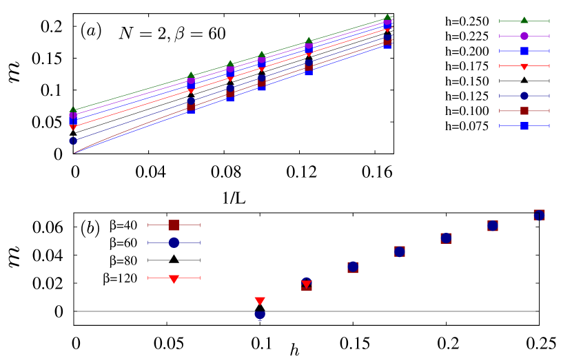
Figure 11: (color online) (a) Magnetization as a function of system size (see Eq. 43). In the ordered phase we have used a second order polynomial form in $1/L$ to extrapolate to the thermodynamic limit. At $h=0.1$ and $h=0.075$ we have set $\beta=120$ and fitted the data to the form $f(x)=aL^{-b}$. (b) Estimated value of the magnetization in the thermodynamic limit.

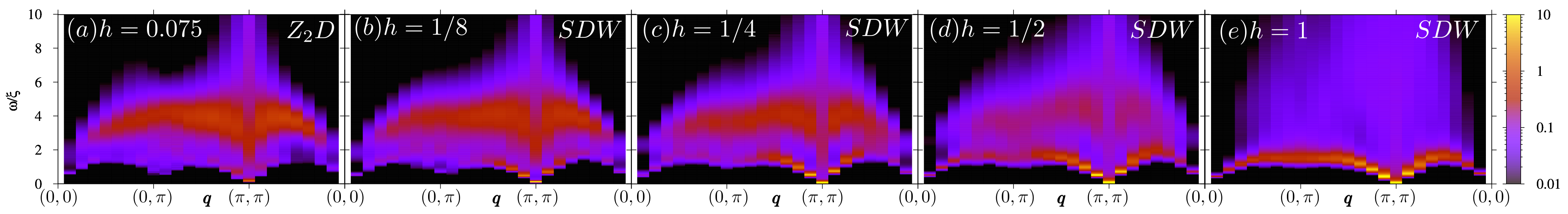
Figure 12: (color online) Dynamical spin structure factor for the $N=2$ model as a function of $h$. For the smallest value of $h$ we have considered $\beta=60$ as opposed to $\beta=40$ for other values of the transverse field. This choice of temperature places us below $T_{c}$ such that $\hat{Q}_{\boldsymbol{i}}\simeq 1$

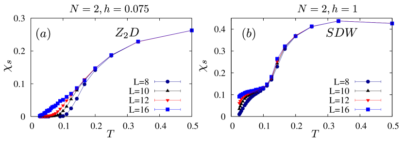
Figure 13: (color online) Uniform spin susceptibility at a) $h=0.075$ (Z₂D phase) and b) $h=1$ (SDW phase).

Let us investigate the zero temperature in the language of spins i.e. in the sector $\hat{Q}_{\boldsymbol{i}}=-1$. We compute the spin-spin correlations given by:

$$S_{\text{Spin}}(\boldsymbol{q},\tau)=\frac{1}{L^{2}}\sum_{\boldsymbol{r},\alpha,\beta}e^{i\boldsymbol{q}\cdot\boldsymbol{r}}\langle\hat{S}^{\alpha}_{\;\;\beta}(\boldsymbol{r},\tau)\hat{S}^{\beta}_{\;\;\alpha}(\boldsymbol{0},0)\rangle.$$ (42)

The local moment of the antiferromagnetic order is then defined as:

$$m=\sqrt{\frac{1}{L^{2}}S_{\text{Spin}}(\boldsymbol{K},0)}.$$ (43)

Note that $\left[\hat{S}^{\alpha}_{\;\;\beta}(\boldsymbol{i}),\hat{Q}_{\boldsymbol{i}}\right]=0$ such that spin excitations do not violate the dynamically generated constraint at $T=0$. Fig. 11 shows the finite size scaling of $m$ for various value of $h$. We see that extrapolation to the thermodynamic limit with a second order form in $1/L$ yields a magnetization which vanishes at $h\simeq 0.1$. Below $h\simeq 0.1$ we have tested for bond dimerized orders but found no positive signal. In this regime, we will interpret our findings in terms of a $\mathbb{Z}_{2}$-Dirac deconfined phase of our effective lattice gauge theory. At $T=0$ where $\hat{Q}_{\boldsymbol{i}}=-1$, the gauge invariant elementary excitations are pairs of spinons tied by a gauge field string of $\hat{Z}_{\boldsymbol{b}}$ operators as well as closed loops of $\hat{Z}_{\boldsymbol{b}}$’s. Below $h\simeq 0.1$ the gauge field is deconfined and the magnetic flux per plaquette is close to $\pi$. In particular one expects the dynamical spin structure factor to bear similarities with the particle-hole continuum of Dirac fermions shown in Fig. 2. In fact the Fig. 2 would correspond to the mean-field theory of the $\mathbb{Z}_{2}$-Dirac deconfined phase.

Fig. 12 plots the dynamical spin-spin correlation functions as a function of $h$. As apparent, in the small $h$ limit we indeed see a continuum of excitations with soft features at wave vectors $(0,\pi)$ and $(\pi,\pi)$ corresponding to transitions between Dirac nodes. As $h$ grows spectral weight accumulates around $\boldsymbol{K}=(\pi,\pi)$ and a distinct spin-density wave feature emerges. As in the $N=1$ case, in the proximity of the transition the continuum of fractionalized excitations is visible at high energies whereas the low energy sector is dominated by the Goldstone mode.

To see the difference between the small $h$ vs large $h$ phase, we also considered the spin-susceptibility,

$$\chi_{s}=\frac{\beta}{N}\left(\langle\hat{\boldsymbol{S}}^{2}\rangle-\langle\hat{\boldsymbol{S}}\rangle^{2}\right).$$ (44)

Some care has to be taken when considering this quantity, since Monte Carlo averages over different $\hat{Q}_{\boldsymbol{i}}$ sectors, and it is only in the low temperature limit that this quantity will correspond to that of the lattice gauge theory. Our results are shown in Fig. 13. As apparent, the two phases have very distinct low energy signatures. Taking into account finite size effects, the $\mathbb{Z}_{2}$-Dirac deconfined phase is characterized by a $\chi_{s}\propto T$ in accord with the mean-field theory of this state. On the other hand, the confined phase is consistent with a constant low temperature spin-susceptibility originating from spin-wave excitations.

V.3 N=3

We will next discuss the $N=3$ model (Eq.1) where alongside a deconfined phase at small $h$ and magnetically ordered phase at large $h$, a spin dimerized state emerges at intermediate values of $h$. As in the $N=1$ case, the $\hat{Q}_{\boldsymbol{i}}$’s order anti-ferromagnetically such that we can pick up the ordering temperature by implementing a small staggered field as in Eq. 27. Our results are plotted in Fig. 14(a) and (b). As expected, anti-ferromagneitc ordering of $\hat{Q}_{\boldsymbol{i}}$ and $\hat{p}_{\boldsymbol{i}}$ occurs at the same energy scale. Being a constant of motion even in the presence of the small staggered chemical potential $\hat{Q}_{\boldsymbol{K}}$ (see Eq. 28) saturates to unity. As a technical aside, we note for values of $h<1/3$ the Monte Carlo autocorrelation time for aforementioned quantities becomes large thus rendering the calculation difficult.

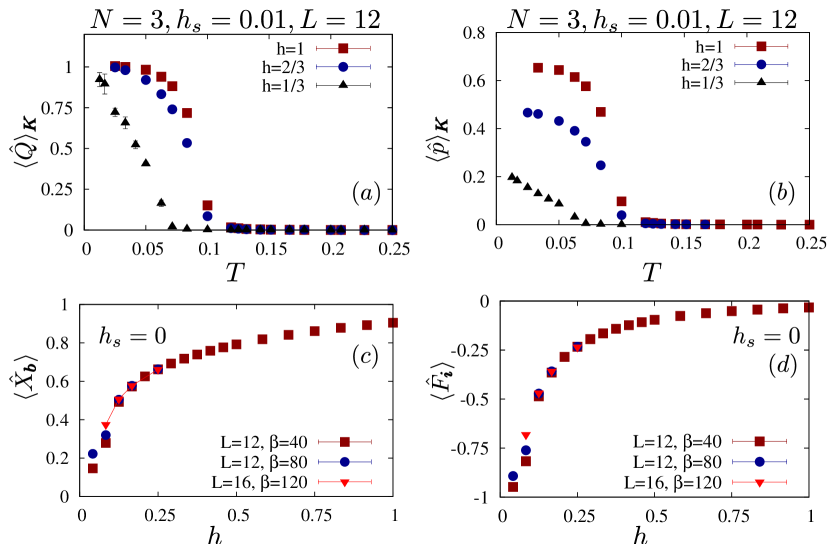
Figure 14: (color online) (a) $\langle\hat{Q}\rangle_{\boldsymbol{K}}=\frac{1}{L^{2}}\sum_{\boldsymbol{i}}e^{i\boldsymbol{K}\cdot\boldsymbol{i}}\langle\hat{Q}_{\boldsymbol{i}}\rangle$ and (b) $\langle\hat{p}\rangle_{\boldsymbol{K}}=\frac{1}{L^{2}}\sum_{\boldsymbol{i}}e^{i\boldsymbol{K}\cdot\boldsymbol{i}}\langle\hat{p}_{\boldsymbol{i}}\rangle$ in the presence of a small staggered chemical potential term which breaks particle-hole symmetry and introduces an antiferromagnetic Zeeman term for the Ising Hamiltonian of Eq. 24. (c) Electric field and (d) Magnetic flux per plaquette as a function of $h$.

In Fig. 14(c) and (d) we plot the magnetic flux as well as the electric field as a function of $h$. Size and temperature effects are large at a small values of $h$. Nevertheless, our data is consistent with absence of level crossing in the ground state quantum numbers since owing to Eq. 33 this would result in a jump in the electric field $\langle\hat{X}_{\boldsymbol{b}}\rangle$.

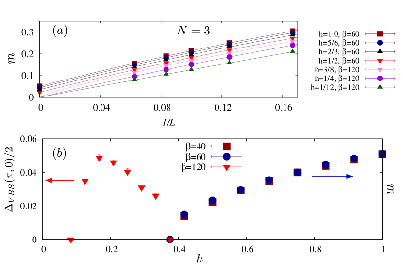
Figure 15: (color online) (a) SU(3) spin staggered moment as a function of system size. The data is consistent with the following choices of fit functions. For $h>3/8$ we have used a second order polynomial in 1/L. At $h=3/8$ we have fitted the data to the form $m(L)=aL^{-(1+\eta)/2}$ to obtain $\eta\simeq 0.64$ which turns out to be substantially larger than the exponent obtained for the J-Q model for the SU(3) case, $\eta\simeq 0.4$ Block et al. (2013). For lower values of $h$ we again use a polynomial fit and impose a zero intercept with the y-axis. In Fig. (b) we plot the extrapolated value of the magnetization as well as of the VBS order parameter. At $h=3/8$ both VBS and SDW order parameters are consistent with a power-law decay.

The anti-ferromagnetic ordering of $\hat{p}_{\boldsymbol{i}}$ along with the constraint that there are on average one and a half electrons per unit cell, gives us two options for the resulting charge ordering:
I. One can place two charges on sub-lattice A and one charge on sub-lattice B. This choice leaves the SU(3) color degree of freedom unquenched. In particular, on sub-lattice A, two SU(3) spins combine to give $3\otimes 3=\overline{3}\oplus 6$ where 3 corresponds to the fundamental representation, $\overline{3}$ to the antisymmetric complex conjugate representation with Young tableau consisting of a single column and two rows and 6 to the symmetric representation with Young tableau consisting of a single row and two columns. Since we are working with fermions, only the $\overline{3}$ representation is relevant and has states given by

$$\Delta^{\dagger}_{\alpha,\boldsymbol{i}}=\frac{1}{2}\epsilon_{\alpha,\beta,\gamma}\hat{c}^{\dagger}_{\beta,\boldsymbol{i}}\hat{c}^{\dagger}_{\gamma,\boldsymbol{i}}.$$ (45)

Here summation over repeated indices, running over the three colors of SU(3), is implied. Neglecting the site index $\boldsymbol{i}$ and assuming that under an infinitesimal SU(3) rotation $\hat{c}^{\dagger}_{\gamma}\rightarrow\left(1+i\epsilon\boldsymbol{e}\cdot\boldsymbol{T}\right)_{\gamma,\delta}\hat{c}^{\dagger}_{\delta}$ with $\boldsymbol{T}$, the vector of Gell-Mann matrices, $\boldsymbol{e}$ a unit vector in $\mathbb{R}^{8}$, and $\epsilon$ a real infinitesimal, one will show that $\Delta^{\dagger}_{\alpha}\rightarrow\left(1-i\epsilon\boldsymbol{e}\cdot\overline{\boldsymbol{T}}\right)_{\alpha,\delta}\Delta^{\dagger}_{\delta}$. On sub-lattice B the single electron corresponds to the fundamental representation of SU(3). With this assignment of representations, Néel states, as well spin-dimerized states can naturally occur. For the Néel state we break the SU(3) symmetry by arbitrarily choosing a color $\alpha$ so as to define the state:

$$|\text{N\'{e}el}\rangle=\prod_{\boldsymbol{i}\in\text{A}}\Delta^{\dagger}_{\alpha,\boldsymbol{i}}\prod_{\boldsymbol{j}\in\text{B}}\hat{c}^{\dagger}_{\boldsymbol{j},\alpha}|0\rangle$$ (46)

Fluctuations around this state will produce spin waves. On the other hand, a possible VBS state with $\boldsymbol{q}=(\pi,0)$ order is given by:

$$|\text{VBS}\rangle=\prod_{\boldsymbol{i},e^{i\boldsymbol{q}\cdot\boldsymbol{i}}=1}\left(\sum_{\alpha=1}^{3}\Delta^{\dagger}_{\alpha,\boldsymbol{i}}c^{\dagger}_{\alpha,\boldsymbol{i}+\boldsymbol{a}_{x}}\right)|0\rangle.$$ (47)

This state remains invariant under SU(3) rotations and thereby defines a singlet.
II. The other charge ordering pattern consistent with the anti-ferromagnetic structure of the $\hat{p}_{\boldsymbol{i}}$’s, corresponds to three particles on sub-lattice B and none on sub-lattice A. This assignment quenches the spin degree of freedom.

One might expect that SDW states which possess low lying Goldstone modes are energetically favorable. Our QMC results are consistent with this expectation. In Fig.15 we plot the equal time spin-spin correlation and corresponding staggered moment $m$. Antiferromagnetic spin ordering is present down to $h\simeq 3/8$. At lower values of $h$, the data is consistent with the vanishing of SDW.

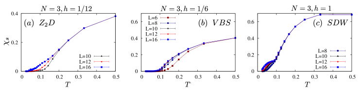
Figure 16: (color online) Uniform spin susceptibility in the Z₂D, VBS and SDW phases.

The uniform spin susceptibility plotted in Fig. 16 gives a very clear account on the nature of the phases one expects as a function of $h$. At $h=1$ and at low temperatures, the data is consistent with the SDW state with constant density of states originating from the Goldstone modes. At $h=1/12$ we observe, similar to $N=2$ case at $h=0.075$, the characteristic spin susceptibility of a Dirac deconfined phase. There is however a distinct intermediate phase possessing no low lying spin excitations. As hinted above, a very natural candidate to account for this is spin-dimerization which breaks the $C_{4}$ lattice symmetry. To verify this, we compute the dimer-dimer correlation functions:

$$\left[S_{\text{VBS}}(\boldsymbol{q})\right]_{\boldsymbol{\delta},\boldsymbol{\delta}^{\prime}}=$$ (48)

$$\frac{1}{L^{2}}\sum_{\boldsymbol{i},\boldsymbol{j}}e^{i\boldsymbol{q}\cdot\left(\boldsymbol{i}-\boldsymbol{j}\right)} \left(\langle\hat{\Delta}_{\boldsymbol{i},\boldsymbol{i}+\boldsymbol{\delta}}\hat{\Delta}_{\boldsymbol{j},\boldsymbol{j}+\boldsymbol{\delta}^{\prime}}\rangle-\langle\hat{\Delta}_{\boldsymbol{i},\boldsymbol{i}+\boldsymbol{\delta}}\rangle\langle\hat{\Delta}_{\boldsymbol{j},\boldsymbol{j}+\boldsymbol{\delta}^{\prime}}\rangle\right)$$

with

$$\hat{\Delta}_{\boldsymbol{i},\boldsymbol{i}+\boldsymbol{\delta}}=\hat{S}^{\alpha}_{\;\;\beta}(\boldsymbol{i})\hat{S}^{\beta}_{\;\;\alpha}(\boldsymbol{i}+\boldsymbol{\delta})$$

. From the above correlation function, we define the dimer order parameter as:

$$\Delta_{VBS}(\boldsymbol{q})=\sqrt{\frac{1}{L^{2}}\text{Tr}\left[S_{\text{VBS}}(\boldsymbol{q})\right]}.$$ (49)

Fig. 17 shows a finite size scaling of the above VBS order parameter at wave vector $\boldsymbol{q}=\left(\pi,0\right)$. Extrapolating to the thermodynamic limit necessarily implies a choice for the fit function. In the parameter range where we observe no low lying spin-excitations in the susceptibility, we use a polynomial fit up to second order in $1/L$. This fit indeed confirms long range valence-bond order in the vicinity of $h=1/6$.

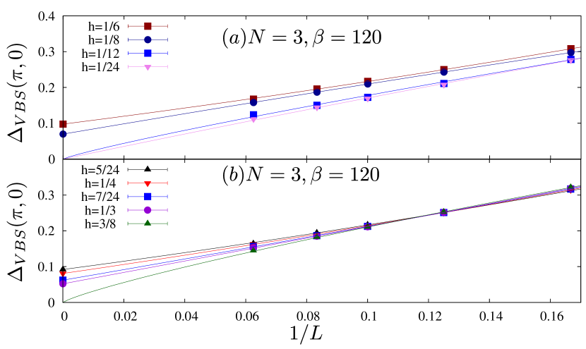
Figure 17: (color online) SU(3) VBS order parameter. At $h=1/12$ corresponding to a rough estimate of the transition from the $\mathbb{Z}_{2}$ Dirac deconfined to the dimerized phase, we fit the data to the form: $aL^{-b}$. The transition from the VBS phase to the SDW occurs approximately at $h=2/3$. For this value of $h$ the data is consistent with a large $\eta=2b-1$ exponent, $\eta\simeq 0.6$ which is larger than the one obtained for the J-Q model at SU(3) $\eta\simeq 0.5$ (see Ref. Block et al. (2013) ).

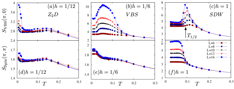
Figure 18: (color online) Temperature dependence of the dimer-dimer and spin-spin correlations in the Z₂D, VBS and SDW phases of the $N=3$ model. The arrow in Fig.(c) corresponds to the energy scale at which $\langle\hat{Q}\rangle_{\boldsymbol{K}}$ plotted in Fig. 14 (a) takes a value of $1/2$ (see Eq. 30).

In Fig. 18 we show the temperature dependence of the VBS and SDW correlation functions at $\boldsymbol{q}=(\pi,0)$ and at $\boldsymbol{q}=\left(\pi,\pi\right)$ respectively and in the Z₂D, VBS and SDW phases. The VBS order breaks the lattice $C_{4}$ symmetry and therefore one correspondingly expects a finite temperature Kosterlitz-Thouless transition below which $S_{\text{VBS}}(\pi,0)$ diverges as a function of system size. The SDW ordering breaks a continuous symmetry and at finite temperatures the real space spin-spin correlations will decay exponentially if the total system size is bigger than the correlation length. In our model, there is also the Ising transition of the $\boldsymbol{Q}_{\boldsymbol{i}}$’s which will feed into the spin and dimer correlation functions. At $h=1$ we can evaluate $T_{1/2}$, $\langle\hat{Q}\rangle_{\boldsymbol{K}}(T_{1/2})=1/2$, from the data shown in Fig. 14(a). This energy scales, which tracks the Ising transition temperature, is shown in Fig. 18 (c). Here, the VBS correlations show strong size effects above the $T_{1/2}$ scale suggesting that the Kosterlitz-Thouless transition temperature exceeds the ordering temperature of the $\boldsymbol{Q}_{\boldsymbol{i}}$’s. At $T_{1/2}$ charge ordering equally occurs (see Fig. 14(b)) leading to a dynamical selection of the representations of SU(3) on each sub-lattice. The fact that at $T_{1/2}$ the antiferromagnetic spin correlations (Fig. 18 (f)) grow agrees with the $3$ and $\bar{3}$ representation pattern. The drop in the VBS order parameter at this energy scale illustrates the competition between these two ordered states and the data at $h=1$ supports dominant SDW correlations in the low temperature limit. We note that the data of Fig. 18 (f) seemingly supports long range order at finite temperature. However, recall that the antiferromagnetic correlation length grows exponentially with inverse temperature Chakravarty et al. (1988) so that when it exceeds our largest lattice size the QMC data falsely suggests long range ordering. Our results at $h=1/6$ in the VBS phase are plotted in Fig. 18 (b),(e). Comparing with the h=1 data set, one observes very similar finite temperature behavior and we again interpret the sharp downturn in the VBS correlation functions as a measure of the Ising transition. However, and in contrast to the $h=1$ data set, the low energy results are consistent with long range dimer order. In the Z₂D phase (see Fig 18 (a),(d)) the Ising transition is again manifest in the sharp upturn in both the dimer and the spin correlations. For this value of the coupling both spin and dimer correlation grow below the Ising transition.

Overall the data is consistent with a deconfined phase at small values of $h$, a valence bond solid at intermediate values of $h$ and finally antiferromagnetic order at large values $h$. The evolution of the order parameters is show in Fig. 15(b). From this we observe that the SU(3) model not only captures a seemingly continuous transition between the $\mathbb{Z}_{2}$ Dirac deconfined and the VBS, similar to the $N=2$ case, but also a transition from the spin-dimerized state (VBS) to the SDW phase. Since we observe no jump in the electric field and the order parameters also evolve continuously, Eq. 33 leads to the conclusion that all transitions are continuous. In particular, the VBS and SDW phases is then expected to be an instance of a deconfined quantum critical point occurring at $h\simeq 3/8$, similar to those found in quantum magnets Lou et al. (2009). The low energy theory for this transition has been argued to be three complex bosons coupled to a non-compact U(1) gauge field (non-compact CP₂ theory) Senthil et al. (2004). Within our limited system sizes we were not able to confirm the literature value of the exponents Block et al. (2013); Harada et al. (2013). Note however that even for the largest values of $L$ in Ref. Harada et al. (2013) the $\nu$ exponent has still not converge. We notice that irrespective of the value of $\nu$, $\beta_{m}<\beta_{VBS}$ where $\beta$ corresponds to the order parameter exponent. This inequality between $\beta_{m}$ and $\beta_{VBS}$ is seemingly consistent with Fig. 15(b) where VBS order parameter rises more sharply compared to the SDW as one moves away from the transition on the two sides.

Fig. 19 plots the evolution of the spin dynamical structure factor as a function of $h$. As for the SU(2) case, $\left[\hat{Q}_{\boldsymbol{i}},\hat{S}^{\beta}_{\;\;\alpha}(\boldsymbol{j})\right]=0$ such that intermediate states in the Lehmann representation of the zero temperature spectral function do not violate the dynamically generated constraint.

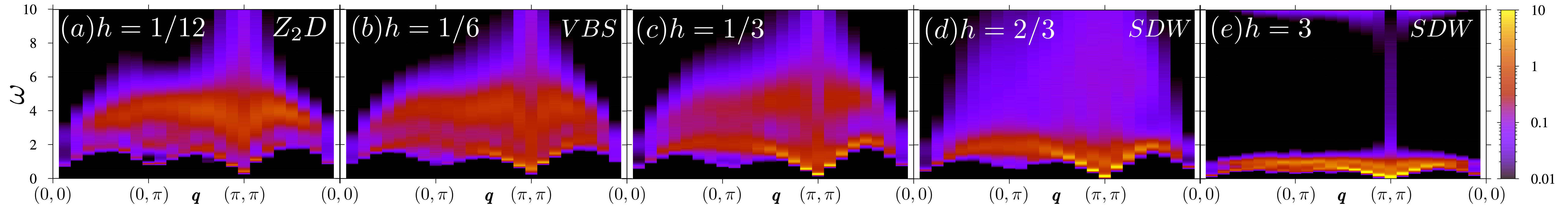
Figure 19: (color online) Dynamical spin structure factor for the SU(3) model. The simulations were carried out on a $16\times 16$ lattice at $\beta=30$ for $h\geq 1/6$ and at $\beta=60$ for $h=1/12$.

Since we are running through two phase transition in rather close proximity, we have to disentangle features stemming from the $\mathbb{Z}_{2}$ Dirac deconfined phase and from the deconfined quantum critical point. The characteristic of the Z₂D phase at $h=1/12$ is the spinon continuum, the high energy features of which are very visible across the transition, and in the VBS phase ($h=1/6$) but then fade away when entering the SDW phase ($h\geq 3/8$) and are completely absent in the strong coupling limit at $h=3$. At this coupling strength, one observes a pronounced Goldstone mode in the vicinity of $\boldsymbol{K}=(\pi,\pi)$ accounting for the spin order. Starting from this point and turning down the transverse field $h$ results in a loss of weight of the spin wave mode. Upon close inspection, one equally sees that it shifts to higher energies.

Another striking feature is the overall broadness of the spectral function in the vicinity of the antiferromagnetic wave vector and in proximity of the VBS to SDW transition at $h\simeq 1/3$. Qualitatively, this is consistent with a deconfined quantum critical point which is characterized by a large value of the anomalous dimension $\eta$ characterizing a complete breakdown of well defined quasiparticles at criticality. Of course, since the spin susceptibility at criticality is expected to be of the form:

$$\chi(\boldsymbol{q},\omega)\simeq\frac{1}{\left(c^{2}|\boldsymbol{q}-\boldsymbol{Q}|^{2}-\omega^{2}\right)^{1-\eta/2}}$$ (50)

with $c$ the spin velocity, any non-zero $\eta$ implies absence of quasiparticles. However at a conventional Wilson-Fisher fixed point in 2+1 dimensions, which describes a phase transition between an SDW and a featureless paramagnet in the Heisenberg universality class $\eta\approx 0.036$ Wang et al. (2006); Campostrini et al. (2002), and correspondingly there are essentially no broad features visible in $S(\bm{q},\omega)$ Lohöfer et al. (2015). For the SU(3) J-Q model which shows a deconfined critical point, $\eta\simeq 0.4$ Block et al. (2013) . We note that the Z₂D to SDW transition observed in the SU(2) model is equally characterized by a large value anomalous exponent which within the $\epsilon$-expansion reads $\eta=0.8$. In the vicinity of the transition (see Fig. 12 a) and b)) broad features at the antiferromagnetic wave vector are again apparent.

The data set at $h=3$ (see Fig. 19e)) corresponds to the strong coupling limit where the spin wave velocity vanishes as $\frac{1}{2Nh}$. Upon comparison between the data sets of Fig. 19d) and e) one notices a marked reduction of the spin wave velocity. Another striking feature of the data, is the lack of a sharp spin-wave mode as seen in the SU(2) case at our strongest coupling (see Fig. 12e)). In fact in the vicinity of the $\boldsymbol{q}=(\pi,0)$, one detects two distinct features. We interpret this in terms of charge fluctuations around the mean-field spin-density wave state of Eq. 46. Setting $\alpha=1$ in this equation and applying Hamiltonian $\hat{H}_{\infty}$ will generate spin-flip excitations on bonds with $\alpha=2,3$. This set of excitations lead to the spin-density wave mode. One will however equally generate charge fluctuations where one site of the bond is left empty and the other accommodates three particles. We interpret the additional features observed in the data in terms of these charge fluctuations. At $h=\infty$ spin and charge excitations are degenerate and the spin wave velocity as well as the energy cost of the charge excitation are tied to the same scale $\frac{1}{2Nh}$ such that we cannot dissociate both features. Furthermore one easily sees that such charge fluctuations do not occur in the SU(2) case, where we observe a sharp spin-wave mode (Fig.12e).

VI Summary and Future Directions

Perhaps the most attractive feature of our model (Eq.1) is that despite its simplicity and the absence of fermion sign problem, the phase diagram is rather rich (Fig.1) and features several highly entangled phases and quantum phase transitions. In particular, in the $\mathbb{Z}_{2}$ deconfined phase, topological degrees of freedom, namely, the dynamically generated $\mathbb{Z}_{2}$ gauge field is coupled to gapless fermions. From an entanglement perspective, the $\mathbb{Z}_{2}$ Dirac phase will result in sharp universal footprints in their entanglement structure and this provides an attractive opportunity to apply some of the recently developed techniques to calculate entanglement entropies and entanglement spectrum Grover (2013); Assaad et al. (2014); Broecker and Trebst (2014); Assaad (2015); Drut and Porter (2015). Specifically, the universal part of the entanglement in the $\mathbb{Z}_{2}$ Dirac phase is expected to follow the relation $\gamma_{Z_{2}D}=\gamma_{D}+\log(2)$ where $\gamma_{D}$ is the universal value for the same shaped region in a regular Dirac phase Yao and Qi (2010). It would be similarly interesting to study the entanglement structure at the transition from Z₂D to symmetry broken phases for $N=2$ and $N=3$, as well as at the deconfined critical point between SDW and VBS.

The transitions from Z₂D phase to the SDW/SC for $N=2$ and to VBS for $N=3$ are rather exotic since they appear to be continuous while involving both symmetry breaking, and confinement of the gauge field . We don’t have an understanding of these transitions and it’s a worthwhile direction to pursue.

Although our model is not microscopically motivated by any specific material(s), the resulting phenomenology does share several features with spin-liquid candidate materials Kagawa et al. (2005); Han et al. (2012); Shimizu et al. (2003); Itou et al. (2008) which also exhibit broad, non-quasiparticle features in their excitation spectrum. It is also worth noting that there have been recent proposals for realizing dynamical gauge-matter theories in cold atomic lattices where instead of imposing the gauge constraint as a penalty term, the Hamiltonians such as ours (Eq.1) appear naturally due to angular momentum conservation Zohar et al. (2013, 2016).

Our model features an interesting interplay of several symmetries – an extensive number of conserved operators $\hat{Q}_{\boldsymbol{i}}$ that anti-commute with the particle-hole symmetry, as well as continuous O(2N) symmetry that allows one to perform sign free Monte Carlo for all N. The particle-hole symmetry is the reason that our model hosts a finite temperature transition where $\hat{Q}_{\boldsymbol{i}}$ spontaneously orders leading to an effective ‘Gauss’s law’ for a $\mathbb{Z}_{2}$ gauge-matter theory, unlike a conventional gauge theory Kogut and Susskind (1975); Senthil and Fisher (2000) where the Gauss’s law is imposed explicitly on the Hilbert space. Contrast this also with 2D Toric code Kitaev (2003) where the Gauss’s law is imposed energetically by explicitly adding a term that is proportional to $\sum_{\bm{i}}\hat{Q^{\prime}}_{\boldsymbol{i}}=\sum_{\bm{i}}\hat{X}_{\boldsymbol{i},\boldsymbol{i}+\boldsymbol{a}_{x}}\hat{X}_{\boldsymbol{i},\boldsymbol{i}-\boldsymbol{a}_{x}}\hat{X}_{\boldsymbol{i},\boldsymbol{i}+\boldsymbol{a}_{y}}\hat{X}_{\boldsymbol{i},\boldsymbol{i}-\boldsymbol{a}_{y}}$. Since this term breaks the $\hat{Q^{\prime}}_{\boldsymbol{i}}\rightarrow-\hat{Q^{\prime}}_{\boldsymbol{i}}$ symmetry explicitly, there is no finite temperature transition in the 2D Toric code. The fields $\hat{Q}_{\boldsymbol{i}}$ in our model are of course classical in the sense that they are conserved and don’t have any dynamics. It would be desirable to extend the idea of studying deconfined phases of gauge theories without imposing the gauge constraint to other gauge groups as well, particularly to the case of $U(1)$ gauge theory relevant to several spin-liquid candidates. Imposing gauge constraint numerically is often challenging, and our results indicate that at least in certain gauge theories, is not necessarily required.

On the above note, it would also be interesting to explore Toric code Kitaev (2003) like Hamiltonians with inbuilt $\hat{Q^{\prime}}_{\boldsymbol{i}}\rightarrow-\hat{Q^{\prime}}_{\boldsymbol{i}}$ symmetry, and study the implications of the melting of the Gauss’s law at finite temperature. This could be especially interesting in 4D Toric code where there exist finite temperature quantum memory Dennis et al. (2002). Is the quantum memory lost as soon as the thermal expectation value $\langle\hat{Q^{\prime}}_{\boldsymbol{i}}\rangle$ vanishes?

In our models, the finite temperature transition corresponding to the ordering of $\hat{Q}_{\boldsymbol{i}}$ coincided with spontaneous breaking of particle-hole symmetry for all values of $N$. This is because $\langle\hat{X}_{\boldsymbol{i},\boldsymbol{i}+\boldsymbol{a}_{x}}\hat{X}_{\boldsymbol{i},\boldsymbol{i}-\boldsymbol{a}_{x}}\hat{X}_{\boldsymbol{i},\boldsymbol{i}+\boldsymbol{a}_{y}}\hat{X}_{\boldsymbol{i},\boldsymbol{i}-\boldsymbol{a}_{y}}\rangle\neq 0$. It is interesting to contemplate the possiblity of a phase where this is not the case such that $\hat{Q}_{\boldsymbol{i}}$ order while the spatial correlation functions of $\hat{p}_{\boldsymbol{i}}$ are short-ranged. Consider for example the model:

$$\hat{H}=\sum_{\left<\boldsymbol{i},\boldsymbol{j}\right>}\left[\hat{Z}_{\langle\boldsymbol{i},\boldsymbol{j}\rangle}\left(\hat{c}^{\dagger}_{\boldsymbol{i}}\hat{c}_{\boldsymbol{j}}+\text{H.c.}\right)+u\,\hat{Q}^{\prime}_{\boldsymbol{i}}\hat{Q}^{\prime}_{\boldsymbol{j}}\right]+v\sum_{\boldsymbol{i}}\hat{Q}_{\boldsymbol{i}}$$ (51)

where $\hat{Q}^{\prime}_{\boldsymbol{i}}=\hat{X}_{\boldsymbol{i},\boldsymbol{i}+\boldsymbol{a}_{x}}\hat{X}_{\boldsymbol{i},\boldsymbol{i}-\boldsymbol{a}_{x}}\hat{X}_{\boldsymbol{i},\boldsymbol{i}+\boldsymbol{a}_{y}}\hat{X}_{\boldsymbol{i},\boldsymbol{i}-\boldsymbol{a}_{y}}$. One can implement a $\hat{Q}^{\prime}_{\boldsymbol{i}}\rightarrow-\hat{Q}^{\prime}_{\boldsymbol{i}}$ symmetry in the above Hamiltonian by demanding that $\hat{H}$ be invariant under the transformation $\hat{U}^{-1}\hat{H}\hat{U}$ where $\hat{U}=\prod^{\prime}_{\langle\boldsymbol{i},\boldsymbol{j}\rangle}\hat{Z}_{\langle\boldsymbol{i},\boldsymbol{j}\rangle}\prod_{{\boldsymbol{i}}}\hat{P}_{\boldsymbol{i}}$ where the prime on the first product denotes that it is taken over all vertical (horizontol) links either only for even rows (columns) or only for odd rows (columns). This transformation takes $\hat{Q}^{\prime}_{\boldsymbol{i}}\rightarrow-\hat{Q}^{\prime}_{\boldsymbol{i}}$, $\hat{Q}_{\boldsymbol{i}}\rightarrow\hat{Q}_{\boldsymbol{i}}$ and $\hat{X}_{\boldsymbol{i},\boldsymbol{j}}\rightarrow-\hat{X}_{\boldsymbol{i},\boldsymbol{j}}$. Therefore, even though $\langle\hat{Q}_{\boldsymbol{i}}\rangle\neq 0$ in this model, the order parameter for the charge-ordering, namely, $\langle\hat{p}_{\boldsymbol{i}}\rangle$ will be non-zero only if the $\hat{U}$ symmetry is spontaneously broken. A phase where $\hat{Q}_{\boldsymbol{i}}$ order while $\hat{p}_{\boldsymbol{i}}$ remain disordered would necessarily involve interesting entanglement between the fermions and the Ising degrees of freedom because one requires that $\langle\hat{X}_{\boldsymbol{i},\boldsymbol{i}+\boldsymbol{a}_{x}}\hat{X}_{\boldsymbol{i},\boldsymbol{i}-\boldsymbol{a}_{x}}\hat{X}_{\boldsymbol{i},\boldsymbol{i}+\boldsymbol{a}_{y}}\hat{X}_{\boldsymbol{i},\boldsymbol{i}-\boldsymbol{a}_{y}}\hat{p}_{\boldsymbol{i}}\rangle\neq 0$ while $\langle\hat{p}_{\boldsymbol{i}}\rangle=0$.

The $N=3$ model has the richest phase diagram among the models we study. In particular, apart from the continuous transition between Z₂D and VBS, the phase diagram contains two distinct symmetry broken phases, the VBS and the SDW phase. Remarkably, we find that these two phases are separated by a second order transition (Fig. 15b), which is thus expected to belong to a non-compact CP₂ universality class Senthil et al. (2004). At this deconfined quantum critical point, we also study the imaginary-time dynamics via the calculation of structure factor $S(\bf{q},\omega)$(Fig. 19, and found a rather broad continuum of excitations, consistent with the theoretical expectation that at this transition, the effective description is in terms of fractionalized ‘spinons’. To our knowledge, the dynamics at the deconfined quantum criticality has not been studied numerically in the past, and given rather distinct features seen in our work, it would be worthwhile to pursue this direction in quantum spin-models where much larger sizes are accessible via bosonic Quantum Monte Carlo such as Stochastic Series Expansion (SSE) Sandvik (2007).

Some cautionary statements are in order for the $N=3$ case. We found it challenging to perform scaling collapse at the both quantum phase transitions, despite no indication of a first-order transition in the behavior of the order parameter. One reason for this could be that the two zero temperature transitions are rather close by in the phase diagram. This is visible in the behavior of the structure factor as $h$ is tuned (Fig. 19) where a diffuse continuum of excitations exists all the way from $h=0$ ($\mathbb{Z}_{2}$ Dirac phase) to $h\sim 1/3$ (VBS to SDW transition). It’s also worth mentioning that the system sizes we are working ($L\leq 16$), are an order of magnitude smaller than the ones for spin-models which exhibit deconfined quantum criticality.

We notice that when $N$ is even, our model does not suffer from sign problem even in the presence of the a non-zero chemical potential on arbitrary lattices. Thus it would be interesting to extend our study to a system with finite density of fermions.

We would like to conclude with a conjecture only tangentially related to the rest of the paper. Consider the Hamiltonian in Eq. 19 for $N=2$ on an arbitrary graph, $\hat{H}_{\infty}=\hat{H}_{\bm{\eta}}+\hat{H}_{\bm{\sigma}}$ where $\hat{H}_{\bm{\eta}}=\sum_{\langle\boldsymbol{i},\boldsymbol{j}\rangle}J_{\boldsymbol{i},\boldsymbol{j}}\left(\hat{\eta}_{\boldsymbol{i}}^{z}\hat{\eta}_{\boldsymbol{j}}^{z}-\frac{1}{2}\left(\hat{\eta}_{\boldsymbol{i}}^{+}\hat{\eta}_{\boldsymbol{j}}^{-}+\hat{\eta}_{\boldsymbol{i}}^{-}\hat{\eta}_{\boldsymbol{j}}^{+}\right)\right)$ and $\hat{H}_{\bm{s}}=\sum_{\langle\boldsymbol{i},\boldsymbol{j}\rangle}J_{\boldsymbol{i},\boldsymbol{j}}\left(\hat{s}_{\boldsymbol{i}}^{z}\hat{s}_{\boldsymbol{j}}^{z}+\frac{1}{2}\left(\hat{s}_{\boldsymbol{i}}^{+}\hat{s}_{\boldsymbol{j}}^{-}+\hat{s}_{\boldsymbol{i}}^{-}\hat{s}_{\boldsymbol{j}}^{+}\right)\right)$. Assuming $J_{\boldsymbol{i},\boldsymbol{j}}\geq 0$, the Hamiltonian $\hat{H}_{\infty}$ is sign problem free on an arbitrary graph because one can use Hubbard-Stratanovich decomposition to write the partition function as a sum of non-negative fermion determinants. On the other hand, considering its decomposition into spin-Hamiltonians $\hat{H}_{\bm{\eta}}$ and $\hat{H}_{\bm{s}}$, only $\hat{H}_{\bm{\eta}}$ is sign problem free on an arbitrary graph due to all non-positive off-diagonal elements in a local basis. Since $\left[\bm{\eta},\bm{S}\right]=0$, the simulatability of $\hat{H}_{\infty}$ suggests that its ground state is likely identical to that of $\hat{H}_{\bm{\eta}}$. That is, in the ground state one expects no singly occupied sites – half of the sites are unoccupied while the other half are doubly occupied, so that only $\hat{H}_{\bm{\eta}}$ acts non-trivially. This leads to the following conjecture: Given a set of $J_{ij}\geq 0$, the ground state energy of $\hat{H}_{-}=\sum_{\langle\boldsymbol{i},\boldsymbol{j}\rangle}J_{\boldsymbol{i},\boldsymbol{j}}\left(\sigma_{\boldsymbol{i}}^{z}\sigma_{\boldsymbol{j}}^{z}-\frac{1}{2}\left(\sigma_{\boldsymbol{i}}^{+}\sigma_{\boldsymbol{j}}^{-}+\sigma_{\boldsymbol{i}}^{-}\sigma_{\boldsymbol{j}}^{+}\right)\right)$ is less than or equal to the ground state energy of $\hat{H}_{+}=\sum_{\langle\boldsymbol{i},\boldsymbol{j}\rangle}J_{\boldsymbol{i},\boldsymbol{j}}\left(\sigma_{\boldsymbol{i}}^{z}\sigma_{\boldsymbol{j}}^{z}+\frac{1}{2}\left(\sigma_{\boldsymbol{i}}^{+}\sigma_{\boldsymbol{j}}^{-}+\sigma_{\boldsymbol{i}}^{-}\sigma_{\boldsymbol{j}}^{+}\right)\right)$. Clearly, on a bipartite graph this conjectured inequality is always saturated. To test this conjecture, we performed exact diagonalization study for systems upto 10 qubits when $J_{ij}$ are chosen randomly from a uniform distribution on $[0,1]$ for a sample size of 1000. We didn’t find any counterexample.

Prior to submission of this paper, we were aware of related work by Snir Gazit, Mohit Randeria and Ashvin Vishwanath . We thank them for sharing their draft.

Acknowledgements: We would like to thank Yin-Chen He, I. Herbut, A. Läuchli, F. Parisen Toldin, S. Trebst, Mike Zaletel and especially Tim Hsieh for discussions. We especially thank Ashvin Vishwanath for pointing out discrepancies in our understanding of the transition between the Z₂D and SDW phase in an earlier draft of the paper.

TG acknowledges startup funds from UCSD. FFA is supported by the German Research Foundation (DFG), under the DFG-SFB 1170 ToCoTronics (Project C01). We thank the Jülich Supercomputing Centre for generous allocation of CPU time. This research was supported in part by the National Science Foundation under Grant No. NSF PHY11-25915.

References

- Bisognano and Wichmann (1975) J. J. Bisognano and E. H. Wichmann, Journal of Mathematical Physics 16, 985 (1975).
- Bisognano and Wichmann (1976) J. J. Bisognano and E. H. Wichmann, Journal of Mathematical Physics 17, 303 (1976).
- Susskind (2004) L. Susskind, An Introduction To Black Holes, Information And The String Theory Revolution: The Holographic Universe (World Scientific Publishing Company, 2004).
- Holzhey et al. (1994) C. Holzhey, F. Larsen, and F. Wilczek, Nuclear Physics B 424, 443 (1994).
- Callan and Wilczek (1994) C. Callan and F. Wilczek, Physics Letters B 333, 55 (1994).
- Calabrese and Cardy (2004) P. Calabrese and J. Cardy, Journal of Statistical Mechanics: Theory and Experiment 2004, P06002 (2004).
- Kitaev and Preskill (2006) A. Kitaev and J. Preskill, Phys. Rev. Lett. 96, 110404 (2006).
- Levin and Wen (2006) M. Levin and X.-G. Wen, Phys. Rev. Lett. 96, 110405 (2006).
- Zhang et al. (2012) Y. Zhang, T. Grover, A. Turner, M. Oshikawa, and A. Vishwanath, Phys. Rev. B 85, 235151 (2012).
- Grover et al. (2011) T. Grover, A. M. Turner, and A. Vishwanath, Phys. Rev. B 84, 195120 (2011).
- Wolf (2006) M. M. Wolf, Phys. Rev. Lett. 96, 010404 (2006).
- Gioev and Klich (2006) D. Gioev and I. Klich, Phys. Rev. Lett. 96, 100503 (2006).
- Swingle (2010) B. Swingle, Phys. Rev. Lett. 105, 050502 (2010).
- Kitaev (2003) A. Kitaev, Annals of Physics 303, 2 (2003).
- Hirsch et al. (1982) J. E. Hirsch, R. L. Sugar, D. J. Scalapino, and R. Blankenbecler, Phys. Rev. B 26, 5033 (1982).
- Blankenbecler et al. (1981) R. Blankenbecler, D. J. Scalapino, and R. L. Sugar, Phys. Rev. D 24, 2278 (1981).
- Troyer and Wiese (2005) M. Troyer and U.-J. Wiese, Phys. Rev. Lett. 94, 170201 (2005).
- Laughlin (1983a) R. B. Laughlin, Phys. Rev. Lett. 50, 1395 (1983a).
- Laughlin (1983b) R. B. Laughlin, Phys. Rev. B 27, 3383 (1983b).
- Yoshioka et al. (1983) D. Yoshioka, B. I. Halperin, and P. A. Lee, Phys. Rev. Lett. 50, 1219 (1983).
- Feiguin et al. (2008) A. E. Feiguin, E. Rezayi, C. Nayak, and S. Das Sarma, Phys. Rev. Lett. 100, 166803 (2008).
- Dagotto et al. (1989) E. Dagotto, J. B. Kogut, and A. Kocić, Phys. Rev. Lett. 62, 1083 (1989).
- Trebst et al. (2007) S. Trebst, P. Werner, M. Troyer, K. Shtengel, and C. Nayak, Phys. Rev. Lett. 98, 070602 (2007).
- Suzuki (1976) M. Suzuki, Progress of Theoretical Physics 56, 1454 (1976), http://ptp.oxfordjournals.org/content/56/5/1454.full.pdf+html .
- Schattner et al. (2015) Y. Schattner, S. Lederer, S. A. Kivelson, and E. Berg, ArXiv e-prints (2015), arXiv:1511.03282 [cond-mat.supr-con] .
- Xu et al. (2016) X. Y. Xu, K. S. D. Beach, F. F. Assaad, and Z. Y. Meng, ArXiv e-prints (2016), arXiv:1602.07150 [cond-mat.str-el] .
- Kogut and Susskind (1975) J. Kogut and L. Susskind, Phys. Rev. D 11, 395 (1975).
- Fradkin and Shenker (1979) E. Fradkin and S. H. Shenker, Phys. Rev. D 19, 3682 (1979).
- Senthil and Fisher (2000) T. Senthil and M. P. A. Fisher, Phys. Rev. B 62, 7850 (2000).
- Senthil et al. (2004) T. Senthil, A. Vishwanath, L. Balents, S. Sachdev, and M. P. A. Fisher, Science 303, 1490 (2004), http://science.sciencemag.org/content/303/5663/1490.full.pdf .
- Sandvik (2007) A. W. Sandvik, Phys. Rev. Lett. 98, 227202 (2007).
- Lou et al. (2009) J. Lou, A. W. Sandvik, and N. Kawashima, Phys. Rev. B 80, 180414 (2009).
- Hsieh et al. (2016) T. H. Hsieh, G. B. Halász, and T. Grover, ArXiv e-prints (2016), arXiv:1604.08591 [cond-mat.str-el] .
- Note (1) In general, one can also allow for the possibility of a background static charge so that the constraint is .
- Su et al. (1980) W. P. Su, J. R. Schrieffer, and A. J. Heeger, Phys. Rev. B 22, 2099 (1980).
- Li et al. (2015) Z.-X. Li, Y.-F. Jiang, S.-K. Jian, and H. Yao, ArXiv e-prints (2015), arXiv:1512.07908 [cond-mat.str-el] .
- Affleck and Marston (1988) I. Affleck and J. B. Marston, Phys. Rev. B 37, 3774 (1988).
- Anderson (1958) P. W. Anderson, Phys. Rev. 112, 1900 (1958).
- Note (2) Note that on a general lattice, the second term would instead be . On a bipartite lattice, such as ours, one can do a unitary transformation to bring it to the form in Eq.20.
- Lieb (1994) E. H. Lieb, Phys. Rev. Lett. 73, 2158 (1994).
- Li et al. (2015) Z.-X. Li, Y.-F. Jiang, and H. Yao, Phys. Rev. B 91, 241117 (2015).
- Assaad and Evertz (2008) F. Assaad and H. Evertz, in Computational Many-Particle Physics, Lecture Notes in Physics, Vol. 739, edited by H. Fehske, R. Schneider, and A. Weiße (Springer, Berlin Heidelberg, 2008) pp. 277–356.
- Sandvik (1998) A. Sandvik, Phys. Rev. B 57, 10287 (1998).
- Beach (2004) K. S. D. Beach, eprint arXiv:cond-mat/0403055 (2004), cond-mat/0403055 .
- Li et al. (2016) Z.-X. Li, Y.-F. Jiang, and H. Yao, ArXiv e-prints (2016), arXiv:1601.05780 [cond-mat.str-el] .
- Yang and Zhang (1990) C. N. Yang and S. C. Zhang, Modern Physics Letters B 04, 759 (1990).
- Note (3) At the level of group structure, O(4) where implements improper rotation, but this distinction will not be relevant for us.
- Wu and Zhang (2005) C. Wu and S.-C. Zhang, Phys. Rev. B 71, 155115 (2005).
- Feldbacher et al. (2003) M. Feldbacher, F. F. Assaad, F. Hébert, and G. G. Batrouni, Phys. Rev. Lett. 91, 056401 (2003).
- Block et al. (2013) M. S. Block, R. G. Melko, and R. K. Kaul, Phys. Rev. Lett. 111, 137202 (2013).
- Note (4) Note that under a particle-hole transformation, the SDW phase will map onto the color superconducting states discussed in Ref. Honerkamp and Hofstetter (2004). There is however an important difference, namely the unpaired flavor forms an CDW rather that a Fermi liquid.
- Note (5) To compute this correlation function we have set: .
- Chakravarty et al. (1988) S. Chakravarty, B. I. Halperin, and D. R. Nelson, Phys. Rev. Lett. 60, 1057 (1988).
- Harada et al. (2013) K. Harada, T. Suzuki, T. Okubo, H. Matsuo, J. Lou, H. Watanabe, S. Todo, and N. Kawashima, Phys. Rev. B 88, 220408 (2013).
- Wang et al. (2006) L. Wang, K. S. D. Beach, and A. W. Sandvik, Phys. Rev. B 73, 014431 (2006).
- Campostrini et al. (2002) M. Campostrini, M. Hasenbusch, A. Pelissetto, P. Rossi, and E. Vicari, Phys. Rev. B 65, 144520 (2002).
- Lohöfer et al. (2015) M. Lohöfer, T. Coletta, D. G. Joshi, F. F. Assaad, M. Vojta, S. Wessel, and F. Mila, Phys. Rev. B 92, 245137 (2015).
- Grover (2013) T. Grover, Phys. Rev. Lett. 111, 130402 (2013).
- Assaad et al. (2014) F. F. Assaad, T. C. Lang, and F. Parisen Toldin, Phys. Rev. B 89, 125121 (2014).
- Broecker and Trebst (2014) P. Broecker and S. Trebst, Journal of Statistical Mechanics: Theory and Experiment 2014, P08015 (2014).
- Assaad (2015) F. F. Assaad, Phys. Rev. B 91, 125146 (2015).
- Drut and Porter (2015) J. E. Drut and W. J. Porter, Phys. Rev. B 92, 125126 (2015).
- Yao and Qi (2010) H. Yao and X.-L. Qi, Phys. Rev. Lett. 105, 080501 (2010).
- Note (6) We thank Ashvin Vishwanath for discussion on this point.
- Kagawa et al. (2005) F. Kagawa, K. Miyagawa, and K. Kanoda, Nature 436, 534 (2005).
- Han et al. (2012) T.-H. Han, J. S. Helton, S. Chu, D. G. Nocera, J. A. Rodriguez-Rivera, C. Broholm, and Y. S. Lee, Nature 492, 406 (2012).
- Shimizu et al. (2003) Y. Shimizu, K. Miyagawa, K. Kanoda, M. Maesato, and G. Saito, Phys. Rev. Lett. 91, 107001 (2003).
- Itou et al. (2008) T. Itou, A. Oyamada, S. Maegawa, M. Tamura, and R. Kato, Phys. Rev. B 77, 104413 (2008).
- Zohar et al. (2013) E. Zohar, J. I. Cirac, and B. Reznik, Phys. Rev. A 88, 023617 (2013).
- Zohar et al. (2016) E. Zohar, J. I. Cirac, and B. Reznik, Reports on Progress in Physics 79, 014401 (2016).
- Dennis et al. (2002) E. Dennis, A. Kitaev, A. Landahl, and J. Preskill, Journal of Mathematical Physics 43, 4452 (2002).
- Note (7) Snir Gazit, Mohit Randeria and Ashvin Vishwanath, arXiv (to appear).
- Honerkamp and Hofstetter (2004) C. Honerkamp and W. Hofstetter, Phys. Rev. B 70, 094521 (2004).