Bilinear condensate in three-dimensional large-$N_{c}$ QCD

Abstract

We find clear numerical evidence for a bilinear condensate in three-dimensional QCD in the ’t Hooft limit. We use a non-chiral random matrix model to extract the value of the condensate $\Sigma$ from the low-lying eigenvalues of the massless anti-Hermitian overlap Dirac operator. We estimate $\Sigma/\lambda^{2}=0.0042\pm 0.0004$ in units of the physical ’t Hooft coupling.

It has been recently shown Karthik and Narayanan (2016a), contrary to expectations (see references in Karthik and Narayanan (2016a)), that QED in three dimensions with parity-invariant coupling to massless two-component fermions does not result in a bilinear condensate for any number of fermion flavors. Further numerical analysis using overlap fermions Karthik and Narayanan (2016b) that preserves the U$(2N_{f})$ global symmetry of the theory on the lattice with $2N_{f}$ flavors of two-component fermions shows that the theory behaves in a scale-invariant manner.

Three-dimensional QCD with SU$(N_{c})$ as the color group and $2N_{f}$ flavors of two-component fermions has also been studied with the aim of finding a critical number of fermion flavors below which the theory is confined and develops bilinear condensate for massless fermions. Analysis of the gap equation Appelquist and Nash (1990) suggests the existence of such a critical number of fermion flavors. A numerical study of the SU$(3)$ gauge theory in the quenched approximation using staggered fermions has shown evidence for a bilinear condensate at finite lattice spacings Damgaard et al. (1998). This issue has been recently studied in Goldman and Mulligan (2016) using the $\epsilon$-expansion about four dimensions.

Consider the theory in the limit of $N_{c}\to\infty$. If the fermions are coupled in a parity-invariant manner, then the fermion determinant is real and positive, and does not contribute to the measure in the $N_{c}\to\infty$ limit, provided $N_{f}$ is kept finite ’t Hooft (1974, 1983). The pure gauge theory in the large-$N_{c}$ limit is in the confined phase at zero temperature, and undergoes deconfinement transition at a temperature $T_{c}$. The continuum reduction Narayanan et al. (2007) implies that the theory in a periodic box of size $\ell_{x}\times\ell_{y}\times\ell_{z}$ is in the confined phase if $\ell_{x},\ell_{y},\ell_{z}>\frac{1}{T_{c}}$ and there is no dependence on the box size. A computation of the string tension using a variational technique Karabali et al. (1998); a numerical evaluation Bringoltz and Teper (2007) at finite values of $N_{c}$ extrapolated to $N_{c}\to\infty$; and a numerical evaluation Kiskis and Narayanan (2008) at large $N_{c}$ using continuum reduction are all in good agreement with each other. Since fermions do not provide a back reaction in the ’t Hooft limit and the theory has a non-zero string tension, we expect massless fermions to develop a non-zero bilinear condensate in the large-$N_{c}$ limit. A numerical study establishing the presence of a bilinear condensate using techniques similar to the ones used in Karthik and Narayanan (2016b) will serve as a sanity check and justify a future numerical study of SU$(N_{c})$ gauge theory coupled to $2N_{f}$ flavors of dynamical fermions and map the critical line in the $(N_{c},N_{f})$ plane that separates the phase where scale invariance is broken from one that is scale-invariant. This is the aim of this brief report.

We used the standard Wilson gauge action and $b$ is the lattice gauge coupling, which is related to the physical ’t Hooft coupling, $\lambda=g^{2}N_{c}$, by

$$b=\frac{1}{a\lambda},$$ (1)

where $a$ is the lattice spacing. We used the primes $N_{c}=7,11,13,17,19,23,29,37,41$ and 47 in this study. We worked on a periodic $L^{3}$ lattice. Based on the numerical studies in Narayanan et al. (2007), we know that $b\in[0.55,0.75]$ is in the confined phase as long as $L\geq 4$. We used five different lattice couplings; $b=$ 0.55, 0.6, 0.65, 0.7 and 0.75 on $4^{3}$ lattice; to study the approach to the continuum limit. We also used $L=4,5$ and 6 at $b=0.75$ to check for any volume dependence. We used overlap fermions with the standard Wilson kernel as described in Karthik and Narayanan (2016b) and studied the behavior of the five low-lying eigenvalues. We used the Cabibo-Marinari SU$(2)$ heat bath along with the SU$(N_{c})$ over-relaxation algorithm Kiskis et al. (2003) to generate 300-500 statistically independent gauge field configurations for the pure gauge theory. Details pertaining to the overlap Dirac operator in three dimensions and the computation of low-lying eigenvalues can be found in Karthik and Narayanan (2016b).

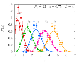
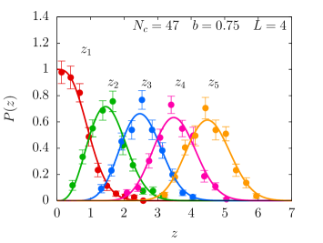
Figure 1: The agreement between the distributions of the five scaled low-lying eigenvalues (data points) of the overlap Dirac operator, $N_{c}L^{3}\Sigma(i,N_{c},L)\Lambda_{i}$, and the distributions from the non-chiral random matrix model (solid curves) is shown. All the data are on $4^{3}$ lattice. Two different $N_{c}$’s are shown : $N_{c}=23$ on the top panel and $N_{c}=47$ on the bottom. Agreement with the non-chiral RMM gets better when $N_{c}$ is increased.

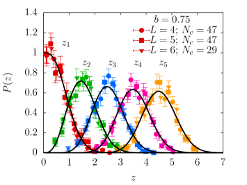
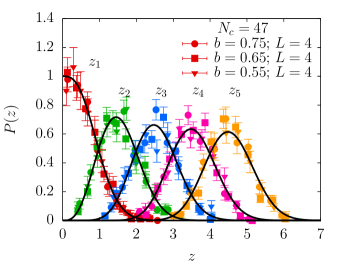
Figure 2: On the top panel, the distributions of the scaled eigenvalues of the overlap Dirac operator at various lattice sizes $L=$ 4, 5 and 6, at the same $b=0.75$, are compared with the distributions from the non-chiral RMM. An agreement is seen independent of the volume. On the bottom panel, such a comparison between the data at $b=$ 0.75, 0.65, 0.55 and the non-chiral RMM distributions is made at the same $L=4$ and $N_{c}=47$. The agreement is seen at all lattice spacings in this study.

The eigenvalues $i\Lambda_{j}$ are associated with an anti-Hermitian operator in the case of overlap fermions. There is no symmetry in three dimensions that pairs up eigenvalues of opposite signs per configuration. The parity symmetry implies that the spectrum is flipped about zero under parity. Therefore, the distribution of eigenvalues will be symmetric around zero. The presence of a bilinear condensate implies a non-zero density at zero eigenvalue. Level repulsion implies that the level spacing of eigenvalues near zero will be inversely proportional to $N_{c}L^{3}$. The individual distributions of the low-lying eigenvalues (ordered by their absolute values) will be governed by an appropriate non-chiral random matrix model (RMM) Verbaarschot and Zahed (1994); Szabo (2001), which in our case will be a Hermitian random matrix model: the matrix elements of a $k\times k$ Hermitian matrix, $H$, are independently and normally distributed with zero mean and a variance of $\pi^{2}/4k$. The spectrum of each randomly generated $H$ will not be symmetric about zero but the distribution will be symmetric on the average since $H$ and $-H$ have the same weight. The distributions of the low lying eigenvalues $z_{j}$ in the RMM model can be obtained using the sinc-kernel and the associated Fredholm determinants Mehta (2004); Nishigaki (2016). We numerically evaluated the eigenvalues of the kernel required for the computation of the determinants and traces of the resolvents, and we were able to determine the distributions of the five lowest eigenvalues $z_{j}$ in the RMM needed for our comparison to a very good accuracy.

The bilinear condensate can be obtained by matching the distribution in the large-$N_{c}$ gauge theory to the RMM model in the large $k$ limit. In theory, for very large $N_{c}$ one should be able to make such a matching for all the eigenvalues using a single number $\Sigma_{\rm lat}(b)$, which is the condensate. In practice, at finite $N_{c}$ we scale the $j$-th eigenvalue by $\Sigma_{\rm lat}(j,N_{c},b,L)$ such that their respective distributions $P_{j}$ match:

$$P_{j}\big{(}\left\{N_{c}L^{3}\Sigma_{\rm lat}(j,N_{c},b,L)\big{\}}\Lambda_{j}\right)=P_{j}\left(z_{j}\right),$$ (2)

where $i\Lambda_{j}$ is the $j$-th eigenvalue of the anti-Hermitian overlap Dirac operator computed in the quenched SU$(N_{c})$ gauge theory on a $L^{3}$ lattice at lattice gauge coupling $b$, and $z_{j}$ is the $j$-th eigenvalue of $H$ in the $k\to\infty$ limit. If a non-zero condensate $\Sigma_{\rm lat}(b)$ is present in the large-$N_{c}$ theory on the lattice, then

$$\Sigma_{\rm lat}(b)=\lim_{N_{c}\to\infty}\Sigma_{\rm lat}(j,N_{c},b,L)\neq 0,$$ (3)

and it should be independent of $j$ (only one scale parameter) and $L$ (lattice volume independence) for large enough $N_{c}$. If a non-zero condensate $\Sigma$ is present in the continuum limit of the large-$N_{c}$ theory, then

$$\frac{\Sigma}{\lambda^{2}}=\lim_{b\to\infty}\Sigma_{\rm lat}(b)b^{2}.$$ (4)

With the intention of obtaining the continuum limit, we consider the quantity, $b^{2}\Sigma_{\rm lat}(b)$, in the following discussion. In Figure 1, we make a comparison of distributions at two different values of $N_{c}$ ($=23$ and $47$), at the finest lattice spacing used in this study. An agreement between the scaled eigenvalues of the overlap operator, and the non-chiral RMM distributions is seen for the low-lying eigenvalues. As one would expect in the presence of a bilinear condensate, this agreement is seen to get better as $N_{c}$ is made larger. Further, we find this agreement with the non-chiral RMM for three different lattice volumes at a fixed lattice coupling as shown in the top panel of Figure 2. The agreement with RMM continues to hold as one changes the lattice coupling as seen in the bottom panel of Figure 2.

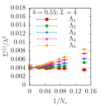
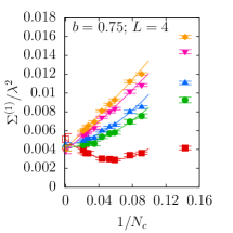
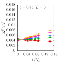
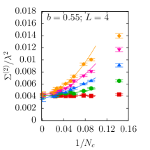
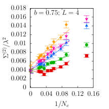
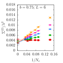
Figure 3: Infinite $N_{c}$ extrapolation of $\Sigma/\lambda^{2}$. The top panels are for $\Sigma^{(1)}/\lambda^{2}$ estimated from the means of the first five low-lying eigenvalues of the overlap Dirac operator, while the bottom ones are for $\Sigma^{(2)}/\lambda^{2}$ estimated from standard deviation of the distributions (refer Eq. (5)). The leftmost panels are at a lattice coupling $b=0.55$ on $L=4$ lattice. The center panels are at $b=0.75$ on $L=4$ lattice. The rightmost panels are at the same $b=0.75$ but on $L=6$ lattice.

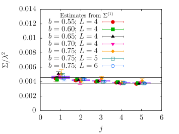
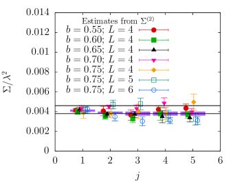
Figure 4: Bilinear condensate at infinite $N_{c}$ as obtained from the mean (top panel), and from the standard deviation (bottom panel) of the $j$-th eigenvalue distribution, for $j=1,\ldots,5$. The purple filled bands over each $j$ are the combined 1-$\sigma$ estimates of $\Sigma(j)/\lambda^{2}$ using the values at different $b$ and $L$, which are shown using symbols. The unfilled bands in the two panels enclose all the estimates of $\Sigma(j)/\lambda^{2}$ at different $j$, thereby giving an estimate of the systematic error in $\Sigma/\lambda^{2}$ due to the large-$N_{c}$ extrapolations and lattice spacing effects.

A convenient way to obtain $\Sigma_{\rm lat}(j,N_{c},b,L)$ is from the mean and central moments of the RMM and $\Lambda$ distributions:

$$\Sigma^{(1)}_{\rm lat}(j,N_{c},b,L)\equiv\frac{1}{N_{c}L^{3}}\frac{\langle z_{j}\rangle}{\langle\Lambda_{j}\rangle};\quad\Sigma^{(n)}_{\rm lat}(j,N_{c},b,L)\equiv\frac{1}{N_{c}L^{3}}\left(\frac{\langle\left(z_{j}-\langle z_{j}\rangle\right)^{n}\rangle}{\langle\left(\Lambda_{j}-\langle\Lambda_{j}\rangle\right)^{n}\rangle}\right)^{1/n}\quad\text{for $n>1$}.$$ (5)

If the distributions agree in the large-$N_{c}$ limit, then the values of $\Sigma^{(n)}_{\rm lat}(j,N_{c},b,L)$ should be the same for all $n$. Since, one requires larger statistics to get reliable values of higher central moments, we restrict ourselves to the mean ($n=1$) and standard deviation ($n=2$) in this paper. In Figure 3, we show the extrapolation of $\Sigma^{(1)}/\lambda^{2}$ and $\Sigma^{(2)}/\lambda^{2}$ to infinite $N_{c}$ using $\Sigma(N_{c}=\infty)/\lambda^{2}+a_{2}/N_{c}+a_{3}/N_{c}^{2}$ ansatz. It is clear that the extrapolations of both $\Sigma^{(1)}$ and $\Sigma^{(2)}$ at various $b$, $L$ and $j$ lead to values $\frac{\Sigma}{\lambda^{2}}\approx 0.004$, significantly away from zero. In Figure 4, we show the various estimates of $\Sigma/\lambda^{2}$ (from different $b$, $L$ and five different eigenvalues) in the large-$N_{c}$ limit. The top panel shows the estimates obtained from $\Sigma^{(1)}$ and the bottom panel for the estimates from $\Sigma^{(2)}$. It is clear that $\Sigma/\lambda^{2}$ from the mean and the standard deviation of the eigenvalue distributions are consistent with each other. The estimates of the condensate using the same $j$-th eigenvalue, $\Sigma(j)/\lambda^{2}$, at the same lattice spacing but different $L$ are consistent within errors, thereby serving as a check on continuum reduction which is a requirement for using smaller $L^{3}$ lattices. A similar consistency is also seen between the estimates of $\Sigma(j)/\lambda^{2}$ at different lattice spacings, which indicates that our estimate is close to the continuum value. Using these independent estimates of $\Sigma(j)/\lambda^{2}$ at different $b$ and $L$, we can get a combined estimate of $\Sigma(j)/\lambda^{2}$, and we have shown these as the different purple filled bands superimposed on the data in Figure 4. We tabulate these values in Table 1 for different $j$. Each of the tabulated entry is an estimate of the condensate in the large-$N_{c}$ limit. It is evident that these $\Sigma(j)/\lambda^{2}$, lie in a narrow range between $0.0038$ and $0.0046$. Even though this range of values is small, it is bigger than the statistical errors in $\Sigma^{(1)}/\lambda^{2}$. We take this small variation in $\Sigma/\lambda^{2}$ between the eigenvalues to be the systematic error in our estimate (which could possibly arise due to higher order $1/N_{c}$ corrections that we are not able to capture and due to lattice corrections), and quote our estimate as

$$\Sigma=(0.0042\pm 0.0004)\lambda^{2}.$$ (6)

This is shown by the unfilled band in Figure 4. We checked that this value is consistent with the estimates from the third central moments of the eigenvalue distributions, which are noisy compared to $\Sigma^{(1)}$ and $\Sigma^{(2)}$. Comparing with the value of string tension, $\sigma$, at $N_{c}\to\infty$ from Karabali et al. (1998); Bringoltz and Teper (2007); Kiskis and Narayanan (2008), we can express

$$\frac{\Sigma}{\sigma}=0.10\pm 0.01.$$ (7)

The result in this paper implies that SU$(N_{c})$ gauge theories coupled to $2N_{f}$ flavors of massless fermions must have a confined phase with a non-zero bilinear condensate. Our future plan is to numerically study such theories using massless overlap fermions with the aim of mapping out the critical line that separates such a phase from a scale invariant phase.

$j$	$\Sigma^{(1)}/\lambda^{2}$	$\Sigma^{(2)}/\lambda^{2}$
1	0.0046(2)	0.0041(1)
2	0.0042(1)	0.0039(1)
3	0.00411(6)	0.0038(2)
4	0.00385(6)	0.0038(2)
5	0.00383(6)	0.0038(2)

Table 1: Estimates of bilinear condensate obtained using $\Sigma^{(1)}(j)$ and $\Sigma^{(2)}(j)$ from the first five low-lying eigenvalues $\Lambda_{j}$ at infinite $N_{c}$, by a combined fit of the estimates of $\Sigma^{(1)}(j)$ and $\Sigma^{(2)}(j)$ at different $L$ and $b$.