Models of the Cosmological 21 cm Signal from the Epoch of Reionization Calibrated with Ly$\alpha$ and CMB Data

Abstract

We present here 21 cm predictions from high dynamic range simulations for a range of reionization histories that have been tested against available Ly$\alpha$ and CMB data. We assess the observability of the predicted spatial 21 cm fluctuations by ongoing and upcoming experiments in the late stages of reionization in the limit in which the hydrogen spin temperature is significantly larger than the CMB temperature. Models consistent with the available Ly$\alpha$ data and CMB measurement of the Thomson optical depth predict typical values of 10–20 mK² for the variance of the 21 cm brightness temperature at redshifts $z=7$–$10$ at scales accessible to ongoing and upcoming experiments ($k\lesssim 1$ cMpc${}^{-1}h$). This is within a factor of a few magnitude of the sensitivity claimed to have been already reached by ongoing experiments in the signal rms value. Our different models for the reionization history make markedly different predictions for the redshift evolution and thus frequency dependence of the 21 cm power spectrum and should be easily discernible by LOFAR (and later HERA and SKA1) at their design sensitivity. Our simulations have sufficient resolution to assess the effect of high-density Lyman limit systems that can self-shield against ionizing radiation and stay 21 cm bright even if the hydrogen in their surroundings is highly ionized. Our simulations predict that including the effect of the self-shielded gas in highly ionized regions reduces the large scale 21 cm power by about 30%.

1 Introduction

Finally unraveling the complete ionization history of hydrogen with high-redshift 21 cm observations is the major science driver of currently operating and planned low-frequency radio telescopes. Achieving the necessary dynamic range for accurate models of the reionization process has thereby been recognized as a key challenge (Trac & Gnedin, 2011). Numerical simulations that aim to be self-consistent in their modeling of ionizing sources and the radiative transfer of ionizing photons in the intergalactic medium (IGM) cannot account for the clustering of sources or the structure of the ionization field on scales greater than $\sim 10$ comoving Mpc (Finlator et al., 2012, 2013; So et al., 2014; Pawlik et al., 2015). On the other hand, simulations that can take these large scale effects into consideration have low spatial and mass resolution and are unable to consistently model small-scale effects such as radiative feedback on ionizing sources and self-shielding of high density regions in the IGM (Lidz et al., 2007; Thomas et al., 2009; Aubert & Teyssier, 2010; Ahn et al., 2012; Shapiro et al., 2012; Bauer et al., 2015; Aubert et al., 2015).

Simulations are nevertheless crucial for the ongoing and upcoming experiments that aim to detect the 21 cm signal from the epoch of reionization (Iliev et al., 2015). The 21 cm brightness distribution is expected to eventually become the ultimate probe of reionization. The design of instruments capable of detecting this signal is guided by its predictions from numerical simulations (e.g., Parsons et al., 2012). Simulations are also crucial in the interpretation of the results of these experiments (Greig et al., 2016), all of which aim to detect the 21 cm signal statistically. Thus, given their relevance, not only should these simulations have a large enough dynamic range to be self-consistent and convergent but they should also be consistent with other currently available constraints on the epoch of reionization. Due to their computational cost, most simulations of the 21 cm signal lack one or both of these properties.

It has been argued that the goal of self-consistent large scale simulation of cosmic reionization is now gradually coming within reach thanks to Moore’s Law (Gnedin, 2014; Gnedin & Kaurov, 2014; Ocvirk et al., 2015; Norman et al., 2015), but semi-numerical and analytical methods of reionization modeling continue to remain attractive for efficient and flexible exploration of the parameter space, especially given the paucity of data at high redshifts (Mesinger & Furlanetto, 2007; Geil & Wyithe, 2008; Choudhury et al., 2009; Mesinger et al., 2011; Kulkarni & Choudhury, 2011; Venkatesan & Benson, 2011; Kuhlen & Faucher-Giguère, 2012; Alvarez & Abel, 2012; Mitra et al., 2013; Zhou et al., 2013; Battaglia et al., 2013; Robertson et al., 2013; Kaurov & Gnedin, 2013; Sobacchi & Mesinger, 2014; Paranjape & Choudhury, 2014; Mitra et al., 2015; Hassan et al., 2016).

In this paper, we combine a high dynamic range cosmological simulation with an excursion set based model for the growth of ionized regions to predict the 21 cm signal during the epoch of reionization. We follow the approach of Choudhury et al. (2015; hereafter CPHB15) to calibrate the simulation parameters such that they reproduce the IGM Lyman-$\alpha$ (Ly$\alpha$) opacity at $z\lesssim 6$ (Fan et al., 2006; Becker et al., 2015; McGreer et al., 2015) as well as the cosmic microwave background (CMB) constraints on the electron scattering optical depth (Planck Collaboration, 2016a, b). The advantage of this approach is that once the reionization history is given, all other quantities of interest—such as the photoionization rate, emissivity of ionizing sources, and the clumping factor of the IGM—can be calculated self-consistently from the simulation box at each redshift. This enables us to simulate concordant models of reionization consistent with a wide variety of observations without losing the dynamic range of our simulations.

CPHB15 applied this method to study the evolution of Ly$\alpha$ emission in high-redshift galaxies by calibrating a “hybrid” cosmological simulation box, which was created by combining a low-resolution cosmological simulation box at large scales with a high-resolution simulation box at small scales. A similar approach was used by Mesinger et al. (2015) to study the evolution of the Lyman-$\alpha$ emitter fraction of high-redshift galaxies. In their approach, a seminumerical scheme was used to obtain the low-resolution simulation. The hybrid box used in CPHB15 formally had very high dynamic range (equivalent to a cosmological simulation with $2\times 5120^{3}$ particles in a 100 $h^{-1}$cMpc box) but did not correctly represent the clustering of matter at scales larger than the size of the small box, which was 10 $h^{-1}$cMpc. Thus from the point of view of deriving the cosmological 21 cm signal, hybrid boxes are of little use as they fail to yield, e.g., the 21 cm power spectrum at scales of interest. The main improvement in the simulation method used in this work is the use of a cosmological hydrodynamical simulation with improved dynamic range.

We follow CPHB15 and consider three different reionization histories for our analysis. One of our reionization histories follows the widely used model of the meta-galactic UV background by Haardt & Madau (2012; hereafter HM12). This model was tuned to match the constraints on reionization from the Wilkinson Microwave Anisotropy Probe (WMAP; Jarosik et al. 2011) and predicts an electron scattering optical depth higher than the recent Planck measurements (Planck Collaboration, 2016a, b). We therefore explore two other reionization histories in which reionization is completed later than in the HM12 model and the electron scattering predictions are consistent with Planck results.

In addition to the evolution of the ionized fraction, the 21 cm signal also depends on the distribution of optically thick systems that are self-shielded from the ionizing radiation. Such systems, which are high-redshift counterparts of the Lyman-limit systems seen in quasar absorption spectra, are usually missed by low resolution simulations. We leverage our high dynamic range to study the effect of these self-shielded regions on the 21 cm signal using a prescription for self-shielding provided by Rahmati et al. (2013). Finally, we consider whether our predicted signal can be observed by five ongoing and upcoming 21 cm experiments. The main aim of the paper is thus to use models that are calibrated to existing data and predict the 21 cm signal and its detectability at different redshifts.

We describe our simulations and the calibration procedure in Section 2. Section 3 presents our predictions for the 21 cm signal and its observability in ongoing and future experiments. We investigate the effect of various assumptions on our results in Section 4 and conclude with a discussion in Section 5. Our $\Lambda$CDM cosmological model has $\Omega_{\mathrm{b}}=0.0482$, $\Omega_{\mathrm{m}}=0.308$, $\Omega_{\Lambda}=0.692$, $h=0.678$, $n=0.961$, $\sigma_{8}=0.829$, and $Y_{\mathrm{He}}=0.24$ (Planck Collaboration, 2014).

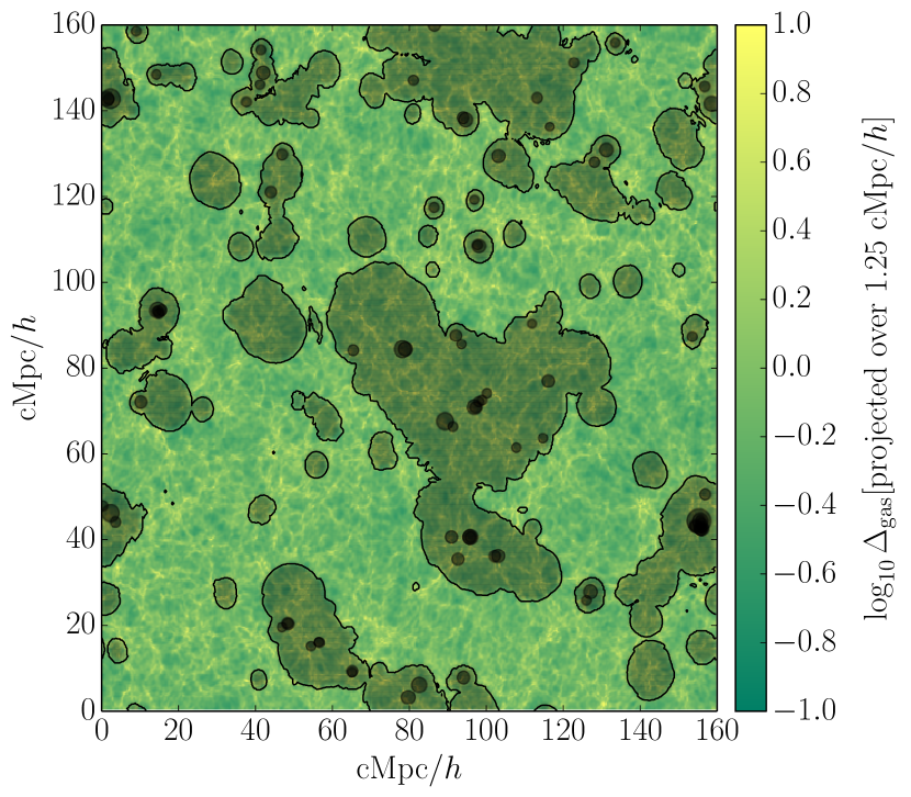
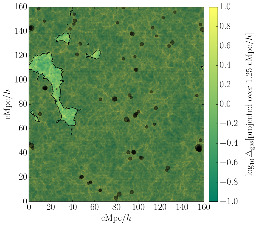
Figure 1: Distribution of gas density at $z=7$. Black symbols denote the locations of centres of masses of dark matter haloes. Shaded areas in both panels show ionized regions identified by the excursion set method. Colour scale shows the gas density. The left panel shows the ionization field for $\zeta_{\mathrm{eff}}=0.5$, which corresponds to $Q_{V}=0.31$. The right panel shows the ionization field for $\zeta_{\mathrm{eff}}=1.0$, which corresponds to $Q_{V}=0.94$.

2 Calibrated Simulations of Cosmic Reionization

Our 21 cm predictions are based on cosmological hydrodynamical simulations with large dynamic range that are part of the Sherwood simulation suite and were run as part of a large (15 million core hour, PI: James Bolton) prace simulation program (Bolton et al., 2016). Sources of ionizing radiation are placed in dark matter haloes identified in the simulation, and an ionization field is obtained using the well-known excursion set approach. This resultant ionization field is then calibrated to a given reionization history, while accounting for residual neutral gas in ionized regions. The reionization history used for calibration is chosen carefully such that it is consistent with a range of Ly$\alpha$ and CMB data. In this manner, our models self-consistently predict the large scale distribution of neutral hydrogen with high resolution for reionization histories consistent with data that constrain the ionization state of hydrogen during the late stages of reionization.

2.1 Large Scale Ionization Field

The Sherwood simulation suite has been run using the energy- and entropy-conserving TreePM smoothed particle hydrodynamical (SPH) code p-gadget-3, which is an updated version of the gadget-2 code (Springel et al., 2001; Springel, 2005). Our base simulation was performed in a cubic box of length 160 $h^{-1}$cMpc on a side. Periodic boundary conditions were imposed. The number of gas and dark matter particles were both initially $2048^{3}$. This corresponds to a dark matter particle mass of $M_{\mathrm{dm}}=3.44\times 10^{7}$ $h^{-1}$M_⊙ and gas particle mass of $M_{\mathrm{gas}}=6.38\times 10^{6}$ $h^{-1}$M_⊙. The softening length was set to $l_{\mathrm{soft}}=3.13$ $h^{-1}$ckpc. The simulation evolves the gas and dark matter density fields from $z=99$ to $z=2$. We use the QUICK_LYALPHA flag in p-gadget-3 in order to speed up the simulation: gas particles with temperature less than $10^{5}$ K and overdensity of more than a thousand times the mean baryon density are converted to collisionless stars and removed from the hydrodynamical calculation (Viel et al., 2004).

In addition to the cosmological evolution of baryons and dark matter, the simulation implements photoionization and photoheating of baryons by calculating the equilibrium ionization balance of hydrogen and helium in a optically thin UV background based on the model of Haardt & Madau (2012), modified so that the resultant IGM temperature agrees with the measurements by Becker et al. (2011). Radiative cooling is implemented by taking into account cooling via two-body processes such as collisional excitation of H i, He i, and He ii, collisional ionization of H i, He i, and He ii, recombination, and Bremsstrahlung (Katz et al., 1996). Likewise, p-gadget-3 also includes inverse Compton cooling off the CMB (Ikeuchi & Ostriker, 1986), which can be an important source of cooling at high redshifts. We ignore metal enrichment and its effect on cooling rates, which is a good approximation for the IGM. In the redshift range relevant to this paper, we use snapshots of the particle positions at $z=10,8,7,$ and $6$. Dark matter haloes are identified using the friends-of-friends algorithm. To calculate power spectra, we project the relevant particles onto a grid to create a density field, using the cloud-in-cell (CIC) scheme. After calculating the power spectrum, we deconvolve the CIC kernel, ignoring small errors due to aliasing on the smallest scales (Cui et al., 2008).

Having obtained the gas density field from the cosmological simulation, we then derive the ionization field corresponding to a distribution of sources with some ionizing emissivity. We assume that the total number of ionizing photons produced by a halo, $N_{\gamma}$, is proportional to its mass $M$. (We further discuss and vary this assumption in Section 4.1.) The minimum halo mass in our simulation is $1.6\times 10^{8}$ $h^{-1}$M_⊙; the maximum halo mass at $z=7$ is $2.1\times 10^{12}$ $h^{-1}$M_⊙. A grid cell at position $\mathbf{x}$ is ionized if the condition

$$\langle n_{\gamma}(\mathbf{x})\rangle_{R}>\langle n_{\mathrm{H}}(\mathbf{x})\rangle_{R}(1+\bar{N}_{\mathrm{rec}}),$$ (1)

is satisfied in a spherical region centred on the cell for some radius $R$ (Furlanetto et al., 2004; Choudhury et al., 2009; Mesinger et al., 2011). Here, the averages are over the spherical region, $n_{\mathrm{H}}$ is the hydrogen number density,

$$n_{\gamma}=\int_{M_{\mathrm{min}}}^{\infty}dM\frac{dn}{dM}N_{\gamma}(M),$$ (2)

where $dn/dM$ is the halo mass function within the spherical region, $M_{\mathrm{min}}$ is the minimum halo mass that contributes ionizing photons, $N_{\gamma}(M)$ is the number of ionizing photons from a halo of mass $M$, and $\bar{N}_{\mathrm{rec}}$ is the average number of recombinations per hydrogen atom in the IGM. The condition in Equation (1) can be recast as

$$\zeta_{\mathrm{eff}}f(\mathbf{x},R)\geq 1,$$ (3)

where

$$f\propto\rho_{m}(R)^{-1}\int_{M_{\mathrm{min}}}^{\infty}dM\frac{dn}{dM}N_{\gamma}(M).$$ (4)

Here $\rho_{m}(R)$ is the average matter density in the sphere of radius $R$. The quantity $f$ is identical to the collapsed fraction $f_{\mathrm{coll}}$ if $N_{\gamma}(M)\propto M$. The parameter $\zeta_{\mathrm{eff}}$ here is the effective ionizing efficiency, which corresponds to the number of photons in the IGM per hydrogen atom in stars, compensated for the number of hydrogen recombinations in the IGM. It is the only parameter that determines the large scale ionization field in this approach. Cells that do not satisfy the criterion in Equation (3) are at least partially neutral, and are assigned an ionized fraction $\zeta_{\mathrm{eff}}f(\mathbf{x},R_{\mathrm{min}})$, where $R_{\mathrm{min}}$ is the length of the cell. We denote the ionized volume fraction in a cell $i$ as $Q_{i}$. The total volume-weighted ionized fraction is then $Q_{V}\equiv\sum_{i}Q_{i}/n_{\mathrm{cell}}$, where $n_{\mathrm{cell}}$ is the number of grid cells.

Figure 1 shows the ionization field in a 1.25 $h^{-1}$cMpc deep slice of our simulation. The colour scale shows the gas density distribution. Black symbols denote the locations of the centres of masses of dark matter haloes. The left and right panels of Figure 1 show the ionization field corresponding to $\zeta_{\mathrm{eff}}=0.5$ and $1$, respectively. As expected, the volume-weighted ionization fraction increases with $\zeta_{\mathrm{eff}}$. Ionized regions prefer overdensities around dark matter haloes. Similar large-scale ionization fields obtained using the excursion set approach have been shown to agree with results of low resolution radiative transfer simulations (Majumdar et al., 2014). However, the excursion set method misses high resolution features, such as self-shielded high density sinks of ionizing photons within the ionized regions (Sobacchi & Mesinger, 2014). A second, related, drawback is that the distribution of ionized IGM in Figure 1 is not calibrated to any observational constraints.

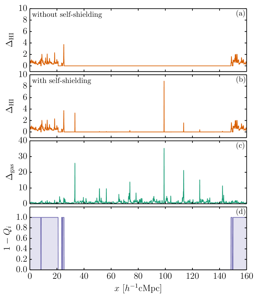
Figure 2: Neutral hydrogen overdensity ($\Delta_{\mathrm{HI}}\equiv n_{\mathrm{HI}}/\bar{n}_{\mathrm{H}}$) along a randomly selected sightline at $z=7$ from the Late/Default model. Panel (a) shows the neutral hydrogen density distribution in absence of self-shielding; panel (b) shows the density distribution when self-shielding is assumed. Panels (c) and (d) show the total gas overdensity ($\Delta_{\mathrm{gas}}\equiv n_{\mathrm{gas}}/\bar{n}_{\mathrm{gas}}$) and the large scale ionization field (here shown as the neutral hydrogen fraction, $1-Q_{i}$) along the same sightline. The region from about $30$ to $150$ $h^{-1}$cMpc is ionized, but high density locations within this region can self-shield.

2.2 Calibration

We calibrate the large scale ionization field obtained by the procedure described above to a chosen reionization history, incorporating inhomogeneities within ionized regions. This is done using the method developed by CPHB15, which we now describe. The aim here is to use the density field from the hydrodynamical simulation and the ionization field from the excursion set approach to derive the spatial distribution of the photoionization rate $\Gamma_{\mathrm{HI}}$ that reproduces a given reionization history. As we will see below, this calibration is equivalent to solving the globally averaged radiative transfer equation at high resolution, without the concomitant numerical cost.

	Model	$L_{\mathrm{box}}$	$N_{\mathrm{gas}}$	$M_{\mathrm{gas}}$	$z_{\mathrm{reion}}$	$\tau$	Minimum halo mass	$N_{\gamma}(M)$
		($h^{-1}$cMpc)		($h^{-1}$M⊙)			(M⊙)
1.	HM12	160	$2048^{3}$	$6.38\times 10^{6}$	6.7	0.084	$2.3\times 10^{8}$	$\propto M_{\mathrm{halo}}$
2.	Late/Default	160	$2048^{3}$	$6.38\times 10^{6}$	6.0	0.068	$2.3\times 10^{8}$	$\propto M_{\mathrm{halo}}$
3.	Very Late	160	$2048^{3}$	$6.38\times 10^{6}$	6.0	0.055	$2.3\times 10^{8}$	$\propto M_{\mathrm{halo}}$
2a.	High Mass	160	$2048^{3}$	$6.38\times 10^{6}$	6.0	0.068	$3.5\times 10^{10}$	$\propto M_{\mathrm{halo}}$
2b.	Nonlinear	160	$2048^{3}$	$6.38\times 10^{6}$	6.0	0.068	$2.3\times 10^{8}$	$\propto M_{\mathrm{halo}}^{1.41}$
2c.	Convergence Run	40	$2048^{3}$	$9.97\times 10^{4}$	6.0	0.068	$2.3\times 10^{8}$	$\propto M_{\mathrm{halo}}$

Table 1: Reionization models considered in this paper. Models 1–3 represent the three reionization histories considered. The “Late/Default” model is our preferred model of reionization. Models 2a and 2b are variations on the Late/Default model. The reionization history in these models is identical to the Late/Default model, but other details have changed. The “High Mass” model has only relatively high mass haloes, while in the “Nonlinear” model, the number of ionizing photons contributed by a halo, $N_{\gamma}(M)$, defined in Equation (2), has a nonlinear dependence on the halo mass. Model 2c uses a higher resolution base simulation together with Late/Default reionization history to check our results for convergence; this model is discussed in Appendix A.

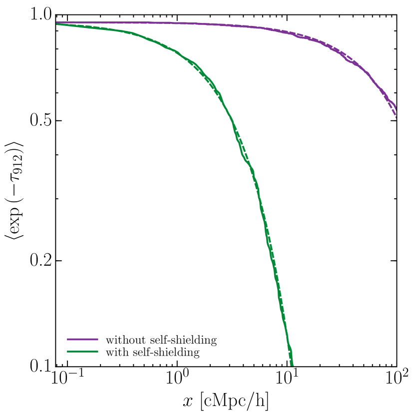
Figure 3: The mean 912 Å transmission along 1000 sightlines in the Late/Default model with and without self-shielding (green and purple curves, respectively). Dashed curves show fits of the form given in Equation (11).

Following CPHB15, we consider three reionization histories for calibration:

• HM12: This model corresponds to the ionization history predicted by the widely used model of the meta-galactic UV background by Haardt & Madau (2012). In this model, ionized regions overlap and the universe is completely reionized at $z=6.7$. The galaxy UV emissivity traces the cosmic star formation history determined from galaxy UV luminosity function measurements at $z>6$ (Robertson et al., 2013). The escape fraction of ionizing radiation increases with redshift. The clumping factor of the high redshift IGM is determined from simulations that are similar to our fiducial simulation but with smaller box sizes so that the resolution is higher by a factor of 4. In this model, quasars and Population III stars make a negligible contribution to the reionization photon budget.

  The HM12 model agrees reasonably well with the background photoionization rate determined from the Ly$\alpha$ forest at $z<6$ (Faucher-Giguère et al., 2009; Becker & Bolton, 2013) and from quasar proximity zones at $z\sim 6$ (Wyithe & Bolton, 2011; Calverley et al., 2011), albeit with notable differences (Puchwein et al., 2015; Chardin et al., 2015). The value of the electron scattering optical depth to the last scattering surface in this model is $\tau=0.084$, which agrees with the WMAP nine-year measurements ($\tau=0.089\pm 0.014$; Hinshaw et al. 2013). This value, however, is inconsistent at more than 1-$\sigma$ level with the much lower value of the optical depth reported by Planck ($\tau=0.058\pm 0.012$; Planck Collaboration 2016b).

• Late/Default: CPHB15 found that the rapid disappearance of Ly$\alpha$ emitters with increasing redshift at $z>6$ suggest a somewhat later reionization than predicted by the HM12 model. We have therefore chosen the “Late” model of CPHB15 as our default reionization model, which we call “Late/Default”. In this model, reionization is complete ($Q_{V}\sim 1$) at $z=6$. The electron scattering optical depth in this model is $\tau=0.068$. This reionization history is consistent with constraints derived by Mitra et al. (2015), and Greig et al. (2016). As we will see the evolution of the neutral hydrogen fraction is also very similar with the default model in the suite of radiative transfer simulations performed by Chardin et al. (2015) that fits the Ly$\alpha$ forest absorption data very well. Chardin et al. (2015) use hydrodynamical simulation boxes with sufficient resolution to resolve Ly$\alpha$ forest absorption features and post-process them with the cosmological radiative transfer code aton (Aubert & Teyssier, 2008). These simulations are able to capture the sudden increase of the ionizing photon mean free path and the mean photoionization rate due to overlap of H ii regions towards the end of reionization. As shown by Chardin et al. (2015), this reionization model also agrees well with the photoionization rate measurements at $z<6$ (Faucher-Giguère et al., 2009; Wyithe & Bolton, 2011; Calverley et al., 2011; Becker & Bolton, 2013). In their radiative transfer simulation, the abundance of sources is thereby consistent with UV luminosity function measurements at $z>6$ (Robertson et al., 2013).

• Very Late: Finally, we also consider the “Very Late” model introduced by CPHB15. In this model, reionization completes at $z=6$ (similar to the Late/Default model), but the ionized fraction $Q_{V}$ evolves more rapidly at $z>6$. The electron scattering optical depth in this case is reduced to $\tau=0.055$. This reionization history is consistent with constraints derived by Mitra et al. (2015) and Greig et al. (2016) and models developed by Khaire et al. (2016).

Table 1 summarizes these three models, together with three variations on the Late/Default model that we consider later in this paper. Each of the above three reionization models is specified by the redshift evolution of the volume-weighted ionization fraction $Q_{V}$. Our simulated ionization field is calibrated to the given reionization model in two steps. In the first step, the effective ionization parameter $\zeta_{\mathrm{eff}}$ is tuned to get the volume-weighted ionization fraction predicted by the reionization model at the corresponding redshift. In the second step, we obtain the photoionization rate distribution within the ionized regions by solving the globally averaged radiative transfer equation

$$\frac{dQ_{V}}{dt}=\frac{\dot{n}_{\mathrm{ion}}}{n_{H}}-\frac{Q_{V}}{t_{\mathrm{rec}}}$$ (5)

for the photoionization rate $\Gamma_{\mathrm{HI}}$.

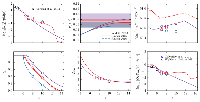
Figure 4: Calibration of our simulation to various reionization models. The red dashed curves show various quantities from Chardin et al. (2015) which is similar to our Late/Default reionization model (shown by the red solid curves). Purple curves show results from Haardt & Madau (2012) and describe our HM12 reionization model. Blue curves show our Very Late reionization model. Purple, red, and blue circles show values of various quantities from our simulation when it is calibrated to the HM12, Late/Default, and Very Late reionization models, respectively. Quantities shown are (clockwise from top left): the mean free path of ionizing photons, Thomson scattering optical depth, rate of ionizing photons, the volume-averaged hydrogen photoionization rate, clumping factor of ionized gas with an overdensity of less than 100, and the volume-weighted ionization fraction. In the top left panel, black squares show measurements of the mean free path of hydrogen-ionizing photons by Worseck et al. (2014). In the top middle panel, the dashed purple line and the associated purple shaded region show the measured value of the Thomson scattering optical depth from WMAP (Hinshaw et al., 2013) and the associated 1$\sigma$ uncertainty, respectively. The red dashed line and shaded region show the measured value of the Thomson scattering optical depth from the 2015 Planck analysis (Planck Collaboration, 2015) with its associated 1$\sigma$ uncertainty. This value was obtained using the Planck CMB power spectra in combination with CMB lensing reconstruction. The blue dashed line and shaded regions show the measured value of the Thomson scattering optical depth from the 2016 Planck analysis (Planck Collaboration, 2016b) with its associated 1$\sigma$ uncertainty. This value was obtained using the Planck CMB polarization and temperature data. In the bottom right panel, black and blue squares show measurements of the hydrogen photoionization rate by Wyithe & Bolton (2011) and Calverley et al. (2011), respectively, from quasar proximity zones.

Note that in Equation (5) the first term on the right hand side is determined by the average comoving photon emissivity $\dot{n}_{\mathrm{ion}}$ which is related to the photoionization rate by (Kuhlen & Faucher-Giguère, 2012; Becker & Bolton, 2013)

$$\dot{n}_{\mathrm{ion}}=\frac{\Gamma_{\mathrm{HI}}Q_{V}}{(1+z)^{2}\sigma_{H}\lambda_{\mathrm{mfp}}}\left(\frac{\alpha_{b}+3}{\alpha_{s}}\right),$$ (6)

where $\alpha_{s}$ is the spectral index of the ionizing sources at $\lambda<912$ Å and $\alpha_{b}$ is the spectral index of the ionizing “background” within ionized regions. The mean free path $\lambda_{\mathrm{mfp}}$ also depends on the photoionization rate $\Gamma_{\mathrm{HI}}$. (We will discuss below how the mean free path is determined.) The $\Gamma_{\mathrm{HI}}$ defined above is the photoionization rate within ionized regions. The corresponding globally averaged value is given by $\Gamma_{\mathrm{HI}}Q_{V}$. We use the same value for the quantity $(\alpha_{b}+3)/\alpha_{s}$ as that used by Haardt & Madau (2012). It is estimated from the model of Haardt & Madau (2012) by computing the ratio $\dot{n}_{\mathrm{ion}}\lambda_{\mathrm{mfp}}/(\Gamma_{\mathrm{HI}}Q_{V})$.

The second term on the right hand side of Equation (5) is also related to the photoionization rate. The recombination time is given by

$$t_{\mathrm{rec}}=\frac{1}{\mathcal{C}\alpha_{R}\chi\bar{n}_{\mathrm{H}}(1+z)^{3}},$$ (7)

where $\mathcal{C}=\langle\rho_{\mathrm{HII}}^{2}\rangle/\langle\rho_{\mathrm{HII}}\rangle^{2}$ is the clumping factor in the ionized regions, $\alpha_{R}$ is the recombination rate, and $\chi=1.08$ is the number of electrons per hydrogen nucleus (assuming that He i is completely ionized in H ii regions). The time scale $t_{\mathrm{rec}}$ is dependent on the photoionization rate via the clumping factor.

It is possible to use Equations (6) and (7) to solve Equation (5) iteratively for the photoionization rate at each point in our simulation box if we are able to calculate the ionized fraction given a photoionization rate and estimate the mean free path. The resultant combination of gas density, source distribution, photoionization rate, and the ionization field are now consistent with the assumed average reionization history. This procedure breaks down in the post-reionization era when $Q_{V}=1$ and $dQ_{V}/dt=0$. In that case, we assume a value of $\Gamma_{\rm HI}$ that is consistent with observations at $z\sim 5$–$6$.

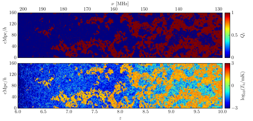
Figure 5: Light cones of the ionized fraction (top panel) and the 21 cm brightness temperature (bottom panel) in the Late/Default model from $z=6$ to $10$. The ionized fraction is obtained using the excursion set method and our hydrodynamical simulations. 21 cm brightness temperature is derived by calibrating the ionization field to the Late/Default reionization history with assumptions for self-shielding in high density regions as suggested by Rahmati et al. (2013).

2.3 Self-shielding

Because of the high resolution of our simulation, it is possible to account for self-shielding and an inhomogeneous photoionization rate distribution in ionized regions. Self shielding is implemented in our simulation during the process of solving Equation (5) for the photoionization rate. For a given photoionization rate $\Gamma_{\mathrm{HI}}$ in a grid cell, the neutral fraction $x_{\mathrm{HI}}\equiv n_{\mathrm{HI}}/n_{\mathrm{H}}$ of the cell is given by

$$x_{\mathrm{HI}}\Gamma^{\mathrm{local}}_{\mathrm{HI}}=\chi n_{H}(1-x_{\mathrm{HI}})^{2}\alpha_{\mathrm{R}},$$ (8)

where $\Gamma^{\mathrm{local}}_{\mathrm{HI}}$ is the local photoionization rate in the cell. This density-dependent photoionization rate is obtained from the background photoionization rate $\Gamma_{\mathrm{HI}}$ using the fitting function obtained by Rahmati et al. (2013) from radiative transfer simulations

$$\frac{\Gamma^{\mathrm{local}}_{\mathrm{HI}}}{\Gamma_{\mathrm{HI}}}=0.98\left[1+\left(\frac{\Delta_{\mathrm{H}}}{\Delta_{\mathrm{ss}}}\right)\right]^{-2.28}+0.02\left[1+\frac{\Delta_{\mathrm{H}}}{\Delta_{\mathrm{ss}}}\right]^{-0.84}.$$ (9)

Here $\Delta_{\mathrm{ss}}$ is a self-shielding density threshold given by (Schaye, 2001; Furlanetto et al., 2005; Rahmati et al., 2013)

$$\Delta_{\mathrm{ss}}=36\left(\frac{\Gamma_{\mathrm{HI}}}{10^{-12}~{}\mathrm{s}^{-1}}\right)^{2/3}\left(\frac{T}{10^{4}~{}\mathrm{K}}\right)^{2/15}\\ \times\left(\frac{\mu}{0.61}\right)^{1/3}\left(\frac{f_{e}}{1.08}\right)^{-2/3}\left(\frac{1+z}{8}\right)^{-3},$$ (10)

where $T$ is the gas temperature, $\mu$ is the mean molecular weight, and $f_{e}=n_{e}/n_{\mathrm{H}}$ is the ratio of free electron and hydrogen number densities. We assume $T=10^{4}$ K in ionized regions.

Figure 2 illustrates the effect of self-shielding by showing the distribution of neutral hydrogen density, total gas density, and the ionization field along a line of sight through the simulation box at $z=7$ for the Late/Default model. Panel (a) shows the H i density distribution in the absence of self-shielding. Panel (b) shows the H i density distribution with self-shielding. Panels (c) and (d) show the total gas overdensity and the large scale ionization field along this line of sight. In the absence of self-shielding the photoionization rate is constant across the large ionized region from $x\sim 25$ to $150$ $h^{-1}$cMpc and the neutral hydrogen fraction is significantly non-zero only outside this region. In contrast, panel (b) shows the neutral hydrogen distribution when self-shielding is applied following the prescription in Equations (8) and (9). Locations within ionized regions now show high neutral hydrogen fraction if they have sufficiently high density as seen, e.g., at around $x\sim 100$ and 120 $h^{-1}$cMpc. Our calibration technique allows us to account for these self-shielded regions.

With a chosen self-shielding criterion, we obtain a neutral hydrogen distribution across the box. This can then also be used to calculate the mean free path of ionizing photons. To estimate the mean free path, we calculate the mean transmission at 912 Å across a large number of sightlines through the box. Figure 3 shows the mean transmission obtained from 1000 sightlines in the box at $z=7$ corresponding to the two self-shielding cases shown in Figure 2. The mean free path $\lambda_{\mathrm{mfp}}$ is then just obtained by fitting the mean transmission by

$$\langle\exp\left(-\tau_{912}\right)\rangle=F_{0}\exp\left(-\frac{x}{\lambda_{\mathrm{mfp}}}\right),$$ (11)

where $x$ is the position along a sightline, as expected for radiative transfer in a highly ionized medium (Rybicki & Lightman, 1985).

Figure 4 shows the result of calibrating our simulation to the HM12 (purple curves and symbols), Late/Default (red curves and symbols), and Very Late (blue curves and symbols) reionization models at redshifts $z=7,8,$ and $10$. The volume-weighted ionization fraction, $Q_{V}$, in the simulation is matched to the model by tuning the effective ionization emissivity parameter $\zeta_{\mathrm{eff}}$. We then get a good agreement between the mean free path and clumping factor in the simulation and the models. This is reflected in the good agreement on the total ionizing photon emission rate, $\dot{n}_{\mathrm{ion}}$ and the photoionization rate. Note that Figure 4 shows the clumping factor of regions with overdensity less than 100 for consistency. In our analysis, we use the clumping factor calculated throughout the ionized regions. At redshift $10$, the low value of the photoionization rate in Equation (10) results in an unrealistically low value of $\Delta_{\mathrm{ss}}$, which can potentially self-shield all the gas in the ionized regions. This problem has been noted by CPHB15. Here we restrict $\Delta_{\mathrm{ss}}\geq 10$ while calibrating our simulation at this redshift. As already discussed the reionization history in our Late/Default model is very similar to the default model in Chardin et al. (2015) . Note that the required ionizing emissivity (upper right panel) in the simulations of Chardin et al. (2015) depends on resolution due to recombinations in the host haloes of the ionizing sources. The simulations of Chardin et al. (2015) are furthermore monochromatic. The ionizing emissivities therefore differ between their work and our model, even though the evolution of the ionized volume fraction is very similar.

3 Cosmological 21 cm Signal

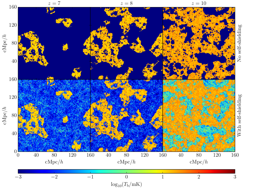
Figure 6: Slices of the 21 cm brightness temperature distribution at $z=7,8,$ and $10$ (left, middle, right columns, respectively) in the Late/Default model, with (bottom row) and without (top row) self-shielding. Self-shielding adds structure in ionized regions.

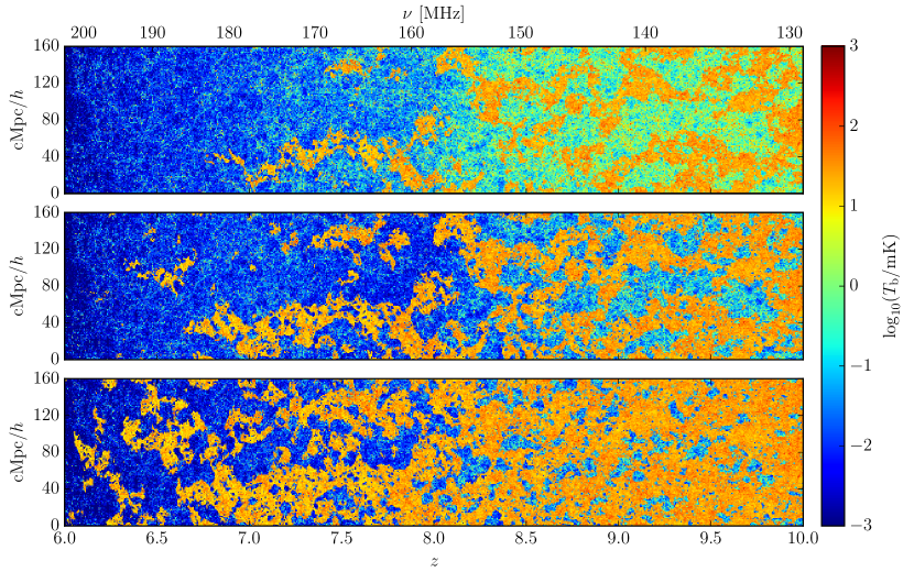
Figure 7: The 21 cm brightness distribution in the HM12 (top panel), Late/Default (middle panel), and Very Late (bottom panel) models.

The calibrated ionization field calculated above can now be used to derive the 21 cm brightness distribution from the epoch of reionization. Due to the calibration procedure described above, this distribution accounts for inhomogeneous recombinations in self-shielded regions of the IGM and is consistent with a variety of other constraints on reionization.

3.1 21 cm brightness temperature

The 21 cm brightness temperature can be approximated as

$$T_{b}(\mathbf{x})=\overline{T}_{b}x_{\mathrm{HI}}(\mathbf{x})\Delta(\mathbf{x}),$$ (12)

where the mean temperature $\overline{T}_{b}\approx 22\mathrm{mK}[(1+z)/7]^{1/2}$ (Choudhury et al., 2009). The above relation does not account for the fluctuations in the spin temperature, i.e., it implicitly assumes that the spin temperature is much greater than the CMB temperature and that the Ly$\alpha$ coupling is sufficiently complete throughout the IGM. These conditions are likely met in the redshift range considered here, when the global ionized fraction is greater than a few per cent (Pritchard & Loeb, 2012; Ghara et al., 2015).

Figure 5 shows light cones through the ionization field and 21 cm brightness distribution in our simulation from $z=6$ to $10$ for the Late/Default reionization model. The horizontal span of the figure is $\sim 1200$ $h^{-1}$cMpc, corresponding to the comoving distance from $z=6$ to $10$. As expected, the neutral regions are the brightest in 21 cm, but there are also self-shielded regions with $T_{b}\sim 1$–$10$ mK within the ionized regions. The number of 21 cm bright regions increases with redshift. It should be noted here that given a reionization history the resultant morphology of the ionized regions in this model is not unique; it is dictated by our assumptions that the total ionizing photon contribution of a halo is proportional to its mass, our assumptions about the spectral index of each source, and the mass range of haloes considered. We consider these issues in greater detail in Section 4 below.

To understand the influence of recombinations on 21 cm brightness, Figure 6 shows the distribution of the 21 cm brightness temperature in our Late/Default model at redshifts $z=7,8,$ and $10$ with and without self-shielding. To obtain the brightness distribution without self-shielding, we repeat the calibration procedure described in Section 2.2 but force the photoionization rate to be uniform within the ionized regions. For a given volume weighted ionization fraction, this typically results in a higher photoionization rate than the self-shielded case, as the mean free path of ionizing photons is significantly larger in the absence of self-shielded sinks (Figure 3). Note that because our calibration procedure fixes the volume weighted ionization fraction by construction, it leaves the size of the ionized regions unchanged when self-shielding is introduced. As a result, panels in the top and bottom rows of Figure 6 have very similar large scale structure. However, the brightness temperature within ionized regions is significantly higher in the simulations with self-shielding due to the presence of neutral hydrogen in dense regions. As gas density increases as $(1+z)^{3}$ and the photoionization rate decreases, this effect is relatively stronger at higher redshifts.

The light cones of the 21 cm brightness distribution for the three reionization histories with self-shielding are shown in Figure 7. The evolution of ionized regions in the three models is as expected, with an early reionization in the HM12 and rapid but late reionization in the Very Late model. The ionized regions in the HM12 model are relatively brighter than those in the Late/Default and Very Late models because the photoionization rate in the HM12 models falls much more rapidly at high redshifts. The effect of self-shielding is visible in the ionized regions in all three models.

3.2 Power spectra

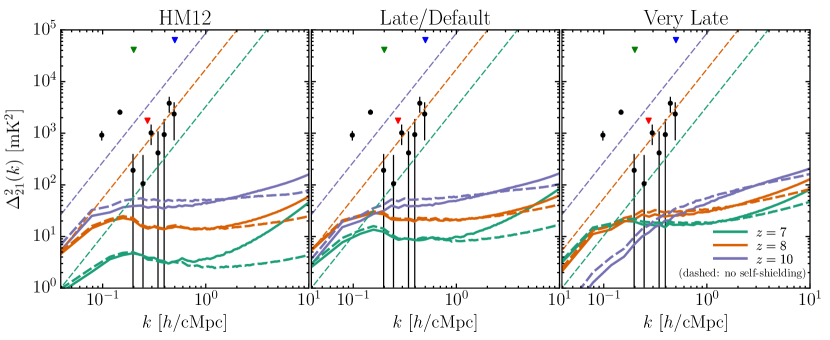
Figure 8: 21 cm power spectra at $z=7$ (green curves), $8$ (orange curves) and $10$ (purple curves) in the three reionization models: HM12 (left panel), Late/Default (middle panel), and Very Late (right panel). Solid curves show the power spectra when self-shielding in ionized regions is accounted for; dashed curves show the power spectra without self-shielding. Blue triangles show upper limits on the power spectrum at $z=8.6$ from GMRT (Paciga et al., 2013). Green triangles show upper limits at $z=9.5$ from MWA (Dillon et al., 2014). Red triangles show upper limits at $z=7.7$ from the 32-element deployment of PAPER (Parsons et al., 2014). Black points with error bars show measurements at $z=8.4$ by the 64-element deployment of PAPER (Ali et al., 2015) with their 2-$\sigma$ uncertainties. Dashed lines show our estimated sensitivity limits for the 64-element deployment of PAPER for same integration time as Ali et al. (2015) at $z=7$ (green), $8$ (orange) and $10$ (purple).

Spatial fluctuations in the 21 cm brightness distribution are conveniently characterized by their power spectrum (Furlanetto et al., 2006). Figure 8 shows the spherically averaged real-space 21 cm power spectra at $z=7,8$ and $10$ in our simulation for the HM12, Late/Default, and Very Late reionization histories. We define the power spectrum as

$$\Delta_{21}^{2}(k)=\frac{k^{3}\langle\tilde{T_{b}^{2}}(k)\rangle}{2\pi^{2}},$$ (13)

where $\tilde{T_{b}}(k)$ is the Fourier transform of the brightness temperature defined in Equation 12 and the average is over the simulation box. Also shown in Figure 8 are the measurements and upper limits from various experiments such as the Giant Metrewave Radio Telescope (GMRT, $z=8.6$; Paciga et al. 2013), Murchison Widefield Array (MWA, $z=9.5$; Dillon et al. 2014), the 32-element deployment of the Precision Array for Probing the Epoch of Reionization (PAPER, $z=7.7$; Parsons et al. 2014), and the 64-element deployment of PAPER ($z=8.4$; Ali et al. 2015). The dashed lines show our estimated sensitivity limits for the 64-element deployment of PAPER for the same integration time as Ali et al. (2015) at $z=7$, $8$ and $10$. We describe how these are derived in Section 3.3 below.

The evolution of the power spectrum is qualitatively familiar (Furlanetto et al., 2006; Pritchard & Loeb, 2012). At large scales the power spectrum amplitude is around 1 to 20 mK², depending on the model. The power spectrum amplitude continuously increases with redshift in the HM12 model (Lidz et al., 2008; Choudhury et al., 2009; Hassan et al., 2016) due to increasing presence of dense, neutral regions. In the Late/Default model, the large scale power first increases from $z=7$ to $8$ and then decreases at $z=10$. This is the “rise and fall” signature of reionization that is visible in the 21 cm power spectrum in the Late/Default model because of the relatively late reionization. This effect is further enhanced in the Very Late model, in which the power spectrum drops from $z=7$ to $10$. At small scales the power spectrum follows the matter spectrum while at intermediate to large scales it deviates from the matter spectrum due to the clustering of ionized regions (Furlanetto et al., 2006). Our predicted 21 cm power spectra are about a factor of three lower than the lowest current experimental upper limits.

Figure 8 also shows the effect of self-shielded regions on the 21 cm power spectra in the three models. Dashed curves in this figure show the 21 cm power when no self-shielding is assumed. In general the effect of self-shielding is to increase 21 cm power at small scales. This is due to increased fluctuations in the 21 cm brightness resulting from the presence of neutral hydrogen in dense regions as seen in Figure 6. This increase in power is seen at all three redshifts in Figure 8 at scales corresponding to $k\gtrsim 1$ cMpc${}^{-1}h$. The enhancement of power generally decreases with increasing redshift between $z=7$ and $10$. At high redshift smaller volume filling factors of ionized regions reduces the impact of self-shielding. In the Late/Default model, at $k=10$ cMpc${}^{-1}h$ the power increment is by about a factor of $\sim 2$ at $z=10$ but it rises to factor of $\sim 5$ at $z=7$.

The effect of self-shielding at large scales is opposite to that at small scales. Here, power is reduced as a result of the reduction in the contrast between the brightness of ionized and neutral regions. This is in qualitative agreement with previous findings in the literature (Sobacchi & Mesinger, 2014; Kaurov & Gnedin, 2015; Hassan et al., 2016). Also, contrary to small scales, the effect of self-shielding on large scales generally increases with increasing redshift. In the Late/Default model, at $k=0.1$ cMpc${}^{-1}h$, the effect at $z=7$ is about 10%, while at $z=10$ the power is reduced by a factor of 30%. Thus, predictions of standard excursion set models of the 21 cm brightness distribution at large scales during the epoch of reionization grow successively worse at higher redshifts.

Parameter	PAPER	MWA	LOFAR	HERA	SKA1-LOW
Number of antennae ($N_{\mathrm{ant}}$)	132	126	48	547	512
Effective collecting area ($A_{\mathrm{eff}}/m^{2}$)	4.0	13.8	526.0	154.0	962.0
Maximum baseline ($b_{\mathrm{max}}/m$)	192.3	2401.9	3475.6	400.0	40286.8
Minimum baseline ($b_{\mathrm{min}}/m$)	4.0	3.72	22.92	14.0	16.8
Largest observable scale at $z=7$ ($k_{\perp}^{\mathrm{min}}/10^{-4}\mathrm{cMpc}^{-1}h$)	3.8	3.5	21.8	13.3	16.0
Largest observable scale at $z=8$ ($k_{\perp}^{\mathrm{min}}/10^{-4}\mathrm{cMpc}^{-1}h$)	3.3	3.1	19.0	11.6	13.9
Largest observable scale at $z=10$ ($k_{\perp}^{\mathrm{min}}/10^{-4}\mathrm{cMpc}^{-1}h$)	2.6	2.4	14.9	9.1	10.9

Table 2: Parameters used for the five experiments considered in this paper. Note that number of antennas in HERA in the final instrument design is 350 (DeBoer et al., 2016). We use SKA parameters obtained by Ghara et al. (2016) which broadly agrees with the baseline distribution given in the latest SKA1-LOW configuration document (http://astronomers.skatelescope.org/documents/; Document number SKA-SCI-LOW-001; date 2015-10-28).

The effect of self-shielding is similar in the HM12 and Very Late models: power is enhanced at small scales and reduced at large scales. The higher the volume filling fraction of ionized regions, the larger is the effect on small scales and smaller is the effect at large scales. At $z=7$ the volume-weighted ionization fraction, $Q_{V}$, in the HM12 model is 0.94, while it is 0.82 in the Late/Default model and 0.58 in the Very Late model. The corresponding difference in the volume filling fraction of neutral hydrogen in the Late/Default and Very Late models increases the predicted 21 cm brightness temperature in the Very Late model as compared to the Late/Default model and decreases it in the HM12 model. This is in turn reflected in the amplitude of the 21 cm power spectra for these models at $z=7$ as seen in Figure 8. At $z=7$ the shape of the power spectrum curves for these three reionization models is very similar but the amplitude increases in the Very Late model relative to the Late/Default model. The power spectrum amplitude in the HM12 is lower than that in the Late/Default model. The effect of self-shielding is also qualitatively similar to that in the Late/Default case: there is a $\sim 10\%$ decrease in the power at large scales ($k\sim 0.1$ cMpc${}^{-1}h$) and a significant increase in the power at small scales ($k\sim 10$ cMpc${}^{-1}h$). The magnitude of this effect is highest in the HM12 model. This can again be understood from the difference in the ionization fractions in the three models.

At redshifts $z=8$ and $10$, the ionization fraction in the Very Late model is much lower than in the Late/Default model. As a result, at $z=8$ the 21 cm power spectrum in the Very Late model already has a lower amplitude than in the Late/Default model at large scales ($k\sim 0.1$ cMpc${}^{-1}h$). At $z=10$, both Late/Default and Very Late model predict lower power spectrum amplitudes relative to the HM12 model at large scales. The result of this behaviour is that in the Very Late model the large scale ($k\sim 0.1$ cMpc${}^{-1}h$) power continuously drops $z=7$ to $z=10$ unlike the power spectrum in the Late/Default model, which shows a rise-and-fall behaviour at large scales. For the Very Late model, the fall in 21 cm brightness does not occur until $z<7$. In the HM12 model, on the other hand, $Q_{V}$ is large enough to push the rise-and-fall signature to redshifts higher than 10. In this model the 21 cm power continuously increases from $z=7$ to $z=10$. A general result is that there is up to 30% decrement in large scale power due to self-shielding.

Note that at post-reionization redshifts ($z<6$), models without self-shielding predict uniformly zero 21 cm signal. At these redshifts, significant amounts of neutral hydrogen are only present in self-shielded systems. However, the overall amplitude of the 21 cm power spectrum is very low at these redshifts and is unlikely to be detected by any of the five experiments considered here.

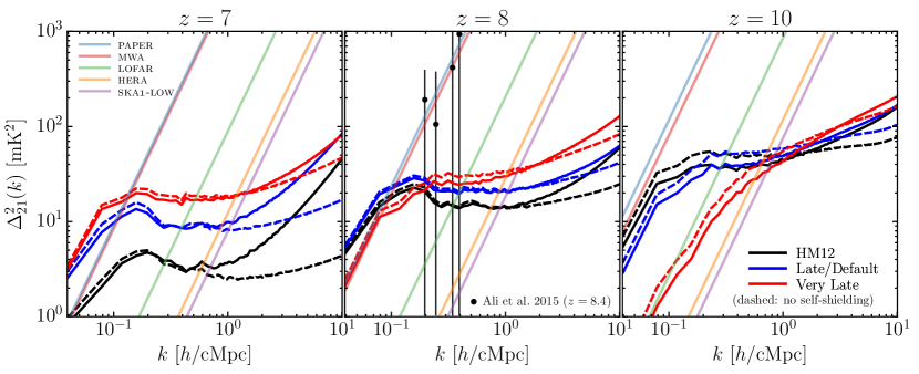
Figure 9: Effect of self-shielding on power spectra on the 21 cm power spectrum at $z=7$ (left panel), $8$ (middle panel), and $10$ (right panel) in our three models. Black, blue, and red curves show power spectra from the HM12, Late/Default, and Very Late models, respectively. Solid curves show power spectra when self-shielding is accounted for. Dashed curves show power spectra without self-shielding. Black points with error bars show measurements at $z=8.4$ by the 64-element deployment of PAPER (Ali et al., 2015) with their 2-$\sigma$ uncertainties. Dashed curves show our estimates of the sensitivities for PAPER (blue), MWA (red), LOFAR (green), HERA (orange), and SKA1-LOW (purple).

3.3 Detecting the 21 cm Power Spectrum

We study here the observational detectability of the 21 cm power spectrum, for five experiments: PAPER (Parsons et al., 2014), MWA (Bowman et al., 2013; Tingay et al., 2013), Low Frequency Array (LOFAR; van Haarlem et al. 2013; Pober et al. 2014), Hydrogen Epoch of Reionization Array (HERA; Pober et al. 2014, DeBoer et al. 2016), and the low frequency instrument from Phase 1 of the Square Kilometre Array (SKA1-LOW; http://astronomers.skatelescope.org). These are listed in Table 2. We assume a system temperature of (Thompson et al., 2007)

$$T_{\mathrm{sys}}=60~{}\mathrm{K}\left(\frac{300~{}\mathrm{MHz}}{\nu_{c}}\right)^{2.25},$$ (14)

and calculate the thermal noise power for an integration over 180 days, assuming a bandwidth of 6 MHz, an observing time of 6 hr per day, and a mid-latitude location.

We follow the method described by Parsons et al. (2012) to calculate experimental sensitivities, which we briefly summarize below. The $uv$ coverage of an interferometric array, obtained by accounting for Earth rotation synthesis of the array’s baselines, is binned in $uv$ pixels. Each pixel then corresponds to an independent sampling of a transverse $k_{\perp}$ mode of the cosmological 21 cm brightness distribution. For each such sampling, the array measures a range of line-of-sight $k_{\parallel}$ modes depending on the bandwidth and frequency resolution. The thermal white noise power for each mode is then given by (McQuinn et al., 2006; Parsons et al., 2012)

$$\Delta_{\mathrm{thermal}}^{2}(k)\approx X^{2}Y\frac{k^{3}}{2\pi^{2}}\frac{\Omega}{2t}T^{2}_{\mathrm{sys}},$$ (15)

where $k=(k_{\perp}^{2}+k_{\parallel}^{2})^{1/2}$, $\Omega$ is the field of view of an element of the array, and $t$ is the total integration time for this $k$-mode. The field of view is given by $\lambda^{2}/A_{\mathrm{eff}}$ where $\lambda=21~{}\mathrm{cm}(1+z)$ and $A_{\mathrm{eff}}$ is the effective area of an interferometric element.

The cosmological quantities $X$ and $Y$ convert from angles and frequencies to comoving distance, respectively, and are given by (Parsons et al., 2012)

$$X\approx 1.9\frac{h^{-1}\mathrm{cMpc}}{\mathrm{arcmin}}\left(\frac{1+z}{10}\right)^{0.2},$$ (16)

and

$$Y\approx 11.5\frac{h^{-1}\mathrm{cMpc}}{\mathrm{MHz}}\left(\frac{1+z}{10}\right)^{0.5}\left(\frac{\Omega_{m}h^{2}}{0.15}\right)^{-0.5}.$$ (17)

The factor of two in Equation (15) assumes that two orthogonal polarizations are measured. To obtain the total thermal noise power, the power from individual modes, given by Equation (15), can be added in quadrature suitably. We assume that every baseline can contribute to the measurement of each $k$-mode, i.e., that the range of $k_{\parallel}$ is broad enough. When multiple non-instantaneously redundant measurements are made, measurements of a $k$-mode can be added up in quadrature thereby reducing the uncertainty in power by the square root of number of measurements. On the other hand, multiple instantaneously redundant measurements of a $k$-mode are equivalent to coherent integration of the temperature measurement. This reduces the uncertainty in power with increasing number of measurements. In this paper, we add all sampling in quadrature. This is in a sense the worst case estimate of the thermal noise.

We first combine redundant measurements in quadrature in each $k$-bin in which the power spectrum is measured. For logarithmic bins of width $\Delta\ln k$, this modifies the thermal noise power of Equation (15) so that

$$\Delta_{\mathrm{thermal}}^{2}(k)\approx X^{2}Y\frac{k^{5/2}}{2\pi^{2}}\left(\frac{1}{B}\right)^{1/2}\left(\frac{1}{\Delta\ln k}\right)^{1/2}\frac{\Omega}{2t}T^{2}_{\mathrm{sys}},$$ (18)

where $B$ is the bandwidth of the observation, which decides the total number of $k$-modes observed for a given resolution. In this paper, we assume $B=6$ MHz for all experiments.

A second combination is performed over measurements of the same $k$-mode by different baselines as they are moved into suitable $uv$-pixels by Earth’s rotation. In order to do this calculation, in what follows, we assume that $N_{\mathrm{ant}}$ antennas are distributed uniformly up to a maximum baseline $b_{\mathrm{max}}$. Thus all redundant measurements are added in quadrature and instantaneously redundant measurements are ignored. Since we assume that each mode can be observed by every baseline, that introduces a term $\propto 1/\sqrt{N}$, where $N$ is number of baselines. Following Parsons et al. (2012), we first sum the sensitivity over rings of $uv$-pixels and then sum over all such rings. This results in a power spectrum given by

$$\Delta_{\mathrm{thermal}}^{2}(k)\approx X^{2}Y\frac{k^{5/2}}{2\pi^{2}}\left(\frac{1}{B}\right)^{1/2}\left(\frac{1}{\Delta\ln k}\right)^{1/2}\\ \times\frac{\Omega}{2t}T^{2}_{\mathrm{sys}}\frac{u_{\mathrm{max}}^{1/2}}{N}\frac{1}{\Omega^{1/4}}\frac{1}{t_{\textrm{per-day}}^{1/2}},$$ (19)

where $u_{\mathrm{max}}$ is the maximum baseline $b_{\mathrm{max}}$ in wavelength units. We assume $t_{\textrm{per-day}}=6$ hr for 120 days. Thus the sensitivity is proportional to $k^{5/2}$.

The thermal noise power spectrum calculated using Equation (19) determines the power spectrum sensitivity of 21 cm experiments. Figure 9 shows the sensitivities of the five experiments described in Section 3 above. Current and upcoming 21 cm experiments are only sensitive to large scales due to limited baselines. As a result, accounting for self-shielding predicts a decrease in the signal to noise ratio for these experiments compared to the predictions from simulations with a more limited dynamic range. None of the experiments are sensitive to 21 cm power for $k\gtrsim 1$ cMpc${}^{-1}h$. SKA1-LOW and HERA have the highest sensitivities primarily due to large number of antenna elements. The signal to noise ratio is about 100 for these two experiments $k\sim 0.1$ cMpc${}^{-1}h$. At $z=7$ and $8$, self-shielding has little effect on the signal to noise ratio, but it is reduced by about a factor of less than two at $z=10$ due to the reduction of signal power as discussed in the previous section. LOFAR has sensitivity for scales corresponding to $k\lesssim 0.2$ cMpc${}^{-1}h$. At $k\sim 0.1$ cMpc${}^{-1}h$, the signal to noise ratio for LOFAR is $\sim 10$ and the fractional reduction at $z=10$ is significant. PAPER and MWA are the least sensitive of the five experiments that we consider in this paper, due to relatively small number of antennas and shorter baselines.

Figure 8 shows our estimated sensitivity limits for the 64-element deployment of PAPER for the same integration time as Ali et al. (2015) at $z=7$, $8$ and $10$ together with their reported measurements. The largest scale observed by the experiments considered here corresponds to the smallest baseline in the array. This is listed in Table 2 and is of the order of $10^{-4}\mathrm{cMpc}^{-1}h$ for all experiments. Note that the sample variance from the limited number of $k$-modes measured in the survey volume also limits the sensitivity of the experiment. The sample variance scales as $\Delta^{2}(k)/\sqrt{N}$ and, due to the small amplitude of the power spectrum, is smaller ($\lesssim 1$ mK²) than the thermal noise at all redshifts for all experiments considered here. Note that we assume perfect foreground subtraction in this discussion. Foreground subtraction will reduce the experimental sensivity (Bernardi et al., 2009; Pober et al., 2013; Dillon et al., 2014). Due to the relatively smooth dependence of astrophysical foregrounds on frequency, this reduction in sensitivity particularly affects small $k$ values.

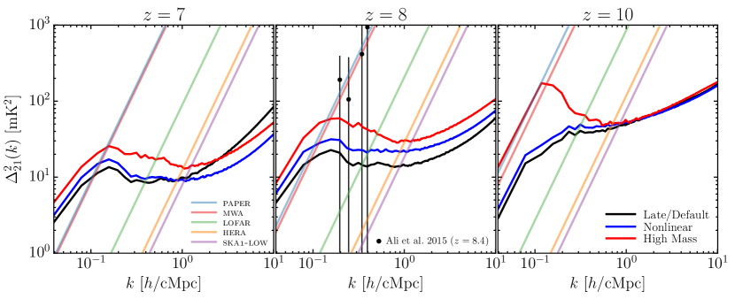
Figure 10: Power spectra of the 21 cm brightness temperature distribution in three models with the Late/Default reionization history at $z=7$ (left panel), $8$ (middle panel) and $10$ (right panel). Black curves correspond the Late/Default model, blue curves show the Nonlinear model, and red curves show the High Mass model. Experimental sensitivities are also shown: PAPER (blue), MWA (red), LOFAR (green), HERA (orange), and SKA1-LOW (purple). Black points with error bars show measurements at $z=8.4$ by the 64-element deployment of PAPER (Ali et al., 2015) with their 2-$\sigma$ uncertainties.

4 Model variations

So far we have assumed that the total number of ionizing photons produced by a halo, $N_{\gamma}$, is proportional to its mass $M$. We have also assumed that sources exist in haloes down to a mass of $\sim 10^{8}$ M_⊙. In this section, we discuss the influence of these assumptions on our results.

4.1 Nonlinear dependence of ionization photon emission rate on halo mass

The assumption that the number of ionizing photons emitted by a halo, $N_{\gamma}(M)$, defined in Equation (2), scales linearly with halo mass can be a bad approximation if, say, the star formation rate (SFR) or the escape fraction of ionizing photons from a halo scales nonlinearly with the halo mass. Galactic outflows and photoionization feedback can influence the dependence of star formation rate on halo mass. In their cosmological radiation hydrodynamical simulations, Finlator et al. (2011) found that feedback not only suppresses star formation in low mass haloes but also affects star formation rate in high mass haloes via hierarchical merging. They found that the SFR scales as $M_{\mathrm{halo}}^{1.41}$ for $M_{\mathrm{halo}}$ between $\sim 10^{8}$ M_⊙ and $10^{10}$ M_⊙. With a halo mass independent escape fraction for ionizing photons, this model was able to match constraints from measurements of the Ly$\alpha$ opacity and the Thomson scattering optical depth.

The blue curves in Figure 10 show the 21 cm power spectrum in our simulation at $z=7$, $8$, and $10$ when the number of ionizing photons emitted by a halo is assumed to scale with halo mass as $M_{\mathrm{halo}}^{1.41}$. Table 1 lists other properties of this model and a slice through the 21 cm brightness field in this model is shown in Appendix B. The model is calibrated to the Late/Default reionization history. Overall, the results are not much different from the Late/Default model presented earlier. The power increases throughout the range of $k$ values shown, by about 20%, because of the additional clustering added to the ionization field by the superlinear halo mass scaling of the number of ionizing photons.

4.2 Effect of feedback

Strong photoionization feedback can prevent star formation in low mass haloes due to photoevaporation of gas (Gnedin & Hui, 1998; Okamoto et al., 2008; Naoz et al., 2009; Gnedin, 2016). Feedback from supernovae is likely even more effective and seems to be a critical ingredient in understanding the abundance of faint galaxies (e.g., Benson et al. 2003, Puchwein & Springel 2013). If feedback is strong in low mass galaxies, the ionizing photon emissivity is dominated by high mass haloes. This can have a significant effect on the topology of the ionized regions (Iliev et al., 2012; Geil et al., 2015). To consider how this affects our prediction for the 21 cm power spectrum, in Figure 10 we consider a model in which only high mass haloes are present (red curves). The minimum halo mass considered in this model is $3.5\times 10^{10}$ M_⊙ which is a factor 152 higher than the minimum halo mass considered in the Late/Default model above. The model is calibrated to the Late/Default reionization history. Table 1 gives further details.

Our results for the effect of very strong feedback on the 21 cm power spectrum are in agreement with previous findings in the literature (McQuinn et al., 2007; Iliev et al., 2012). As seen in Figure 10, due to the enhanced clustering of high mass sources the 21 cm power is enhanced across all scales by factors of a few. For a given volume-weighted ionization fraction $Q_{V}$ the ionization field is now dominated by few large ionized regions. These regions are also more clustered, which increases the 21 cm power. A slice through the 21 cm brightness field in this model is shown in Appendix B. Although broad features in the power spectrum are qualitatively similar to those in the Late/Default model, at redshift $z=10$ the large scale power is enhanced almost ten times to about $100$ mK². Thus reionization histories with strongly clustered bright sources are favourable for the detection of the 21 cm signal. Recently, it has been argued that faint active galactic nuclei (AGN) could contribute significantly to the ionizing background at $z\sim 6$ (Giallongo et al., 2015; Madau & Haardt, 2015; Chardin et al., 2016). Such a scenario would result in an enhancement in the large-scale 21 cm power.

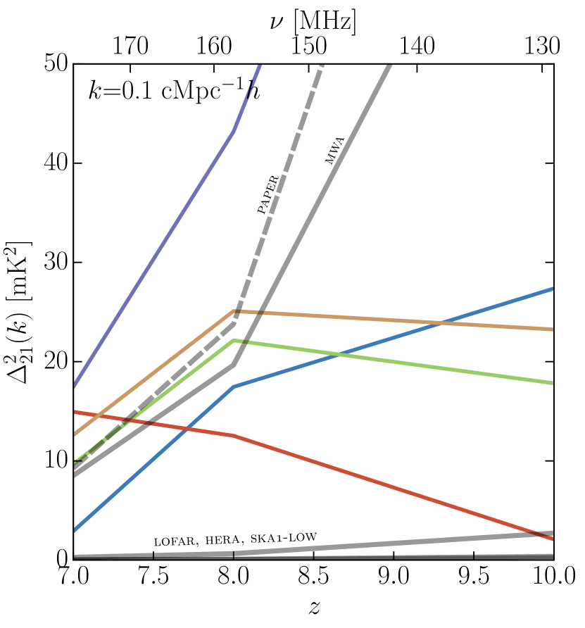
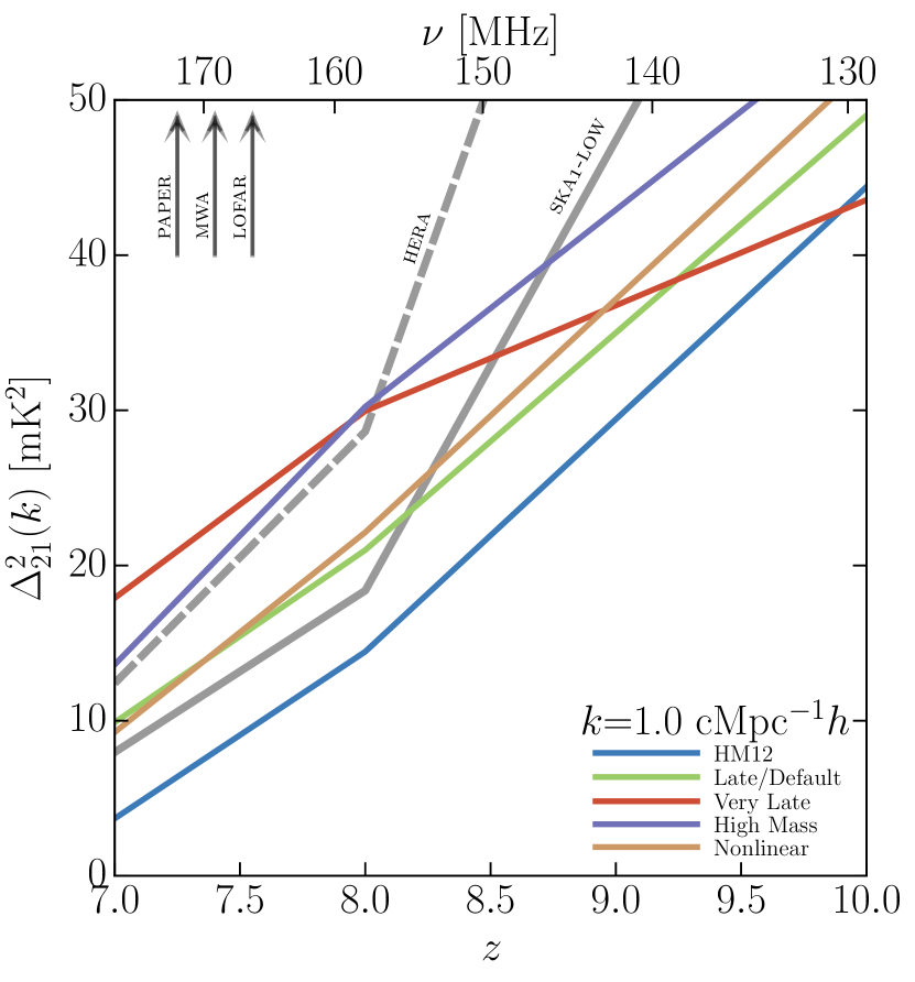
Figure 11: Evolution of 21 cm power at $k=0.1$ cMpc${}^{-1}h$ (left panel) and $k=1.0$ cMpc${}^{-1}h$ (right panel) in all five models presented in this paper: HM12 (blue), Late/Default (green), Very Late (red), High Mass (orange), and Nonlinear (beige). Grey curves show experimental sensitivities at the two scales. At $k=0.1$ cMpc${}^{-1}h$, LOFAR, HERA, and SKA1-LOW, have much lower thermal noise than the signal. At $k=0.1$ cMpc${}^{-1}h$, PAPER, MWA, and LOFAR, have much higher noise than the signal.

4.3 Evolution of power spectra

Figure 11 shows the evolution of 21 cm power from $z=10$ to $z=7$ in all of the reionization models considered in this paper. The left panel shows the evolution of power at $k=0.1$ cMpc${}^{-1}h$ while the right panel shows the power at $k=1.0$ cMpc${}^{-1}h$. The blue, green, and red curves show results from the HM12, Late/Default, and Very Late models respectively. Orange curves show results from the High Mass model calibrated to the Late/Default reionization history. Beige curves shows the Nonlinear model which is also calibrated to the Late/Default reionization history.

We find that the small scale power ($k=1.0$ cMpc${}^{-1}h$) decreases with redshift in all five of our models. The power at these scales is mostly affected by the reducing ionization fraction and photoionization rates. All three models calibrated to the Late/Default reionization history have very similar behaviour at this scale. The High Mass model shows higher amplitude at all redshifts due to the higher clustering of ionizing sources in this model. The HM12 and Very Late models behave differently. The HM12 model has lower power due to smaller neutral fraction, and the Very Late model has higher power.

There is a larger qualitative variation in the behaviour of different models at $k=0.1$ cMpc${}^{-1}h$. The power at this large scale is related to the the variance of the 21 cm brightness temperature distribution that could be measured by the 21 cm experiments (Patil et al., 2014; Watkinson & Pritchard, 2014). The Late/Default model, which agrees with most other reionization constraints, shows the rise and fall signature in the power at this scale. It should be possible for most experiments to detect this. In the redshift range $z=7$–$10$ considered here, the HM12 model only shows the falling part of the power evolution, while the Very Late model only shows the rising part. The High Mass model shows a very rapid increase in power at this scale towards high redshift. As discussed above, for the same volume-weighted ionized fraction the ionization field in this model is dominated by a few large regions around high mass sources. These sources are highly clustered, which correspondingly increases the 21 cm power. The Nonlinear and Late/Default models have similar behaviour at this scale.

5 Conclusions

We have presented here predictions of the spatial distribution of the 21 cm brightness temperature from the epoch of reionization based on high dynamic range cosmological hydrodynamical simulations from the Sherwood simulation suite (Bolton et al., 2016) for reionization histories motivated by constraints from Ly$\alpha$ absorption and emission data as well as CMB data. Our models of the 21 cm signal were obtained by combining the high dynamic range cosmological simulations with excursion set based models of the growth of ionized regions during reionization. This has allowed us to efficiently obtain realistic 21 cm predictions that are firmly anchored in current constraints on how reionization ends and that have sufficient resolution to account for the self-shielding of neutral hydrogen in dense regions within otherwise fully ionized regions. Our main conclusions are as follows:

• Our preferred ‘Late/Default’ model of reionization is consistent with a variety of observational constraints such as the electron scattering optical depth, Ly$\alpha$ opacity, galaxy UV luminosity function at high redshifts, and estimates of the hydrogen photoionization rates from quasar absorption spectra (Chardin et al., 2015). In this model the volume-weighted ionization fraction $Q_{V}$ evolves from 0.37 at $z=10$ to 0.82 at $z=7$ and reionization is complete at redshift $z\sim 6$. The variance of the 21 cm brightness temperature field at large scales accessible to current and upcoming experiments ($k\sim 0.1$ cMpc${}^{-1}h$) reduces from about 20 mK² at $z=10$ to about 10 mK² at $z=7$. Power at these large scales first increases from $z=10$ to $8$, when $Q_{V}$ is 0.65, and then decreases down to $z=7$. The change from the rise to the fall of the signal of reionization, where the 21 cm power peaks occurs when $Q_{V}$ is about 50%, which occurs at about $z=8.5$ in this model. The small scale 21 cm power in this model decreases continuously from about 50 mK² at $z=10$ to 10 mK² at $z=7$ ($k\sim 1$ cMpc${}^{-1}h$). These small scales are, however, unlikely to be accessible to any of the five experiments that we have investigated here, particularly at $z=10$.

• Self-shielding in high density regions within ionized regions affects the 21 cm power in two ways. At the large scales accessible to experiments, self-shielding decreases power by up to 30%. The contribution to the 21 cm power from self-shielded regions tends to be greater at high redshifts unless the ionization fractions are too small. At small scales, self-shielding enhances the 21 cm power by adding structure within ionized regions. This effect is generally stronger at lower redshift due to the larger volume occupied by ionized regions. The enhancement in power at small scales due to self-shielding can be considerable, often even greater than an order of magnitude. Unfortunately, these scales are too small to be detected by the 21 cm experiments considered here. By suppressing power at intermediate scales self-shielding can reduce the rise and fall signature of the epoch of reionization.

• In addition to our favoured Late/Default model, we have considered two other reionization histories. In the reionization history predicted by the widely used HM12 model of the meta-galactic UV background, reionization occurs earlier and the 21 cm signal peaks as early as $z=10$. Otherwise the evolution of the 21 cm brightness distribution is qualitatively similar to the Late/Default model on all scales. As a result of the earlier rise of the ionized volume fraction the large scale power does not show the same rise and fall behaviour in this model between $z=10$ and $7$ due to the relatively larger ionization fraction already at $z=10$. Instead the large scale variance of the 21 cm brightness decreases continuously from about 30 mK² at $z=10$ to about 3 mK² at $z=7$ in this model. Our third reionization history, the ‘Very Late’ model, in which reionization also ends at $z=6$ but starts later than in the other models, also does not show the rise and fall behaviour in the large scale 21 cm power. In this model the large scale power increases continuously from about 2 mK² at $z=10$ to about 15 mK² at $z=7$. The effect of self-shielding on the power spectrum in these two models is qualitatively similar to that in the Late model. In all three cases the effect of self-shielding reduces the large scale 21 cm power by up to 30% and increases the small scale power by factors of up to 10. The latter effect is not accessible at the resolution of the 21 cm experiments we have considered here.

• We have also varied the scaling of the luminosity of the ionizing sources with host halo mass in our models. Our ‘Nonlinear’ model has the same reionization history as the Late/Default model but an ionizing photon rate that is assumed to be a nonlinear function of the halo mass, as, e.g., preferred by the radiation hydrodynamical simulations of Finlator et al. (2011). This moderately strengthens the relative role of high mass haloes compared to low mass haloes during reionization. The results of this model are nearly identical to those from our Late/Default model. We have further considered a higher cut-off in the mass of haloes hosting ionizing sources. In this ‘High Mass’ model, we remove low-mass haloes from our ionization field calculation. This scenario corresponds to strong feedback, completely suppressing star formation in low-mass haloes. We find that although this model is calibrated to the same reionization history as our Late/Default model, suppression of low luminosity sources changes the 21 cm signal significantly. Broad features in the power spectrum are qualitatively similar to those in the Late/Default model, but at redshift $z=10$ the large scale power is enhanced almost ten times to about $100$ mK². Thus reionization histories with strongly clustered bright sources would clearly favour the detection of the 21 cm signal.

• We have derived sensitivity limits of five current and upcoming experiments, PAPER, MWA, LOFAR, HERA, and SKA1-LOW, for the 21 cm power spectrum due to thermal noise and consider the prospects of detecting the reduced large scale 21 cm power spectrum in presence of self-shielding. Assuming perfect foreground removal, LOFAR, HERA, and SKA1-LOW should be able to detect the power spectrum at $k\sim 0.1$ cMpc${}^{-1}h$ at $z=8$ at 20-$\sigma$ to 100-$\sigma$ significance in our Late/Default model, assuming perfect foreground removal. The significance drops at $z=7$ as well as $z=10$ due to changes in the ionization structure and evolution in experimental sensitivities. Detection is more difficult with the first generation experiments PAPER and MWA except at scales larger than our box size of 160 $h^{-1}$cMpc, although foreground removal can be difficult at these large scales (Pober et al., 2014). At $k=0.1$ cMpc${}^{-1}h$, MWA should be able to detect the rise and fall signal of the epoch of reionization at less than 2-$\sigma$, whereas LOFAR should be able to detect it at nearly 10-$\sigma$. Assuming ideal foreground removal, HERA and SKA1-LOW should be able to detect this signature comfortably at excess of 50-$\sigma$. At their design sensitivity LOFAR, HERA and SKA1-LOW should therefore easily discriminate between the ionization histories presented here.

The calibration procedure used in this paper provides a relatively low-cost method of performing high dynamic range simulations of the cosmological 21 cm signal for reionization histories that are well anchored in constraints from other data on how reionization ends. Although self-consistent large scale simulations of cosmic reionization are now gradually becoming possible, the method presented in this paper is valuable for an efficient and flexible exploration of the relevant parameter space that will be necessary for inference from the statistical detection of the 21 cm signal.

Appendix A Convergence test

We have discussed the role of self-shielded structure in the IGM on the large scale ionization field and the 21 cm signal. The base cosmological simulation that we used for our discussion has a box size of 160 $h^{-1}$cMpc and $2048^{3}$ gas and dark matter particles. This corresponds to a dark matter particle mass of $M_{\mathrm{dm}}=3.44\times 10^{7}$ $h^{-1}$M_⊙ and gas particle mass of $M_{\mathrm{gas}}=6.38\times 10^{6}$ $h^{-1}$M_⊙. It is because of this high mass resolution that the simulation was able to resolve the self-shielded structure that is usually missed by radiative transfer simulations of the epoch of reionization. We now check the convergence of our results by deriving the 21 cm signal in a cosmological simulation with higher resolution than our base simulation.

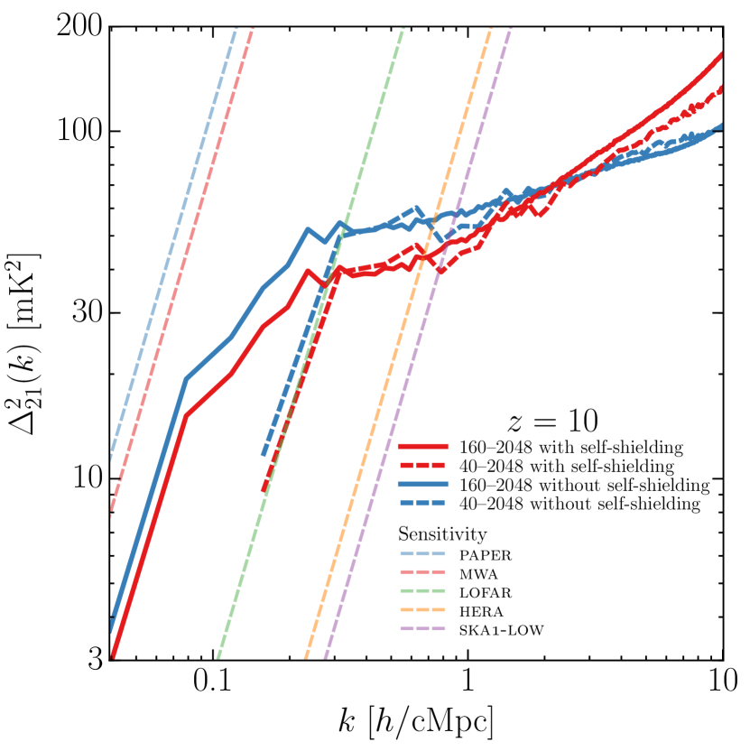
Figure 12: Effect of self-shielding on the 21 cm power spectrum at $z=10$ at two different numerical resolutions. The solid red and blue curves show the power spectra with and without self-shielding, respectively, in our fiducial base simulation, which has a box size of 160 $h^{-1}$cMpc and 2048³ gas particles. The dashed red and blue curves show the power spectra from a simulation with 64 times higher mass resolution. It has a box size of 40 $h^{-1}$cMpc and 2048³ gas particles. Identical reionization histories and halo mass ranges are used to derive these power spectra. The faint dashed curves show experimental sensitivities. Power spectra from the two simulations agree well, suggesting numerical convergence.

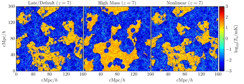
Figure 13: Distribution of 21 cm brightness in the Late/Default (left panel), High Mass (middle panel), and Nonlinear (right panel) models at $z=7$. Each slice has a depth of 78.1 $h^{-1}$ckpc. All three simulations are calibrated to the Late/Default reionization history, which has $Q_{V}=0.82$ at this redshift. Other details of these three models are given in Table 1.

Figure 12 shows the 21 cm power spectrum at $z=10$ taken from a simulation with a box size of 40 $h^{-1}$cMpc and $2048^{3}$ gas and dark matter particles. This corresponds to a dark matter particle mass of $M_{\mathrm{dm}}=5.37\times 10^{5}$ $h^{-1}$M_⊙ and gas particle mass of $M_{\mathrm{gas}}=9.97\times 10^{4}$ $h^{-1}$M_⊙. This simulation thus has a factor of 64 higher mass resolution than our base simulation. The spatial resolution is also higher as the softening length is set to $l_{\mathrm{soft}}=0.78$ $h^{-1}$ckpc. This simulation is also a part of the Sherwood suite of simulations (Bolton et al., 2016). Other details of this simulation are identical to our base simulation. The minimum halo mass in our base simulation is $1.6\times 10^{8}h^{-1}$M_⊙; the maximum halo mass is $2.1\times 10^{12}h^{-1}$M_⊙ at $z=7$. In comparison, the minimum halo mass in the higher resolution simulation is $2.4\times 10^{6}h^{-1}$M_⊙. The maximum halo mass is $4.2\times 10^{10}h^{-1}$ M_⊙ at $z=7$. For Figure 12, a minimum halo mass of $1.6\times 10^{8}h^{-1}$M_⊙ is used when placing the ionizing sources so that the large scale ionization fields can be compared.

In Figure 12, the solid red and blue curves show the 21 cm brightness temperature power spectra in the low resolution simulation with and without the effect of self-shielding respectively. The dashed curves show the corresponding power spectra from the high resolution simulation. Self-shielding is implemented using the same prescription as in Section 2.3. Both simulations are calibrated to the Late/Default model of reionization described in Section 2.2. The power spectrum curves of the low resolution simulation are identical to those from Figure 9. We find that power spectra from the two simulations agree quite well at scales relevant to experiments ($k<1$ cMpc${}^{-1}h$). The effect of self-shielding is also identical in the two simulations on observationally accessible scales. As described in Section 4 self-shielding reduces the large scale power by about a factor of two. This reduction is identical in the two simulations, showing that our self-shielding implementation has converged in the base simulation.

Appendix B 21 cm distribution in the High Mass and Nonlinear models

Figure 13 shows the 21 cm brightness distribution at $z=7$ in the High Mass and Nonlinear models that are discussed in Sections 4.1 and 4.2. The Late/Default reionization model is shown in the left panel for comparison. The middle panel shows the High Mass model in which sources are placed only in high mass haloes. The right panel shows the Nonlinear model in which the source emissivity has a nonlinear dependence on the halo mass. All three models are calibrated to the Late/Default reionization history so that they have $Q_{V}=0.82$ at this redshift.

We find that the 21 cm field in the fiducial Late/Default model is nearly identical to that in the Nonlinear model. This is understandable as the nonlinearity implemented here is mild ($N_{\mathrm{gamma}}\propto M_{\mathrm{halo}}^{1.41}$). The High Mass case shows larger differences from the fiducial Late/Default model. Smaller ionized regions around small mass haloes are not present in the High Mass model. These differences in the ionization fields are reflected in the 21 cm power spectra for these models, which are shown in Figure 10.

References

- Ahn et al. (2012) Ahn K., Iliev I. T., Shapiro P. R., Mellema G., Koda J., Mao Y., 2012, ApJ, 756, L16
- Ali et al. (2015) Ali Z. S., et al., 2015, ApJ, 809, 61
- Alvarez & Abel (2012) Alvarez M. A., Abel T., 2012, ApJ, 747, 126
- Aubert & Teyssier (2008) Aubert D., Teyssier R., 2008, MNRAS, 387, 295
- Aubert & Teyssier (2010) Aubert D., Teyssier R., 2010, ApJ, 724, 244
- Aubert et al. (2015) Aubert D., Deparis N., Ocvirk P., 2015, MNRAS, 454, 1012
- Battaglia et al. (2013) Battaglia N., Trac H., Cen R., Loeb A., 2013, ApJ, 776, 81
- Bauer et al. (2015) Bauer A., Springel V., Vogelsberger M., Genel S., Torrey P., Sijacki D., Nelson D., Hernquist L., 2015, MNRAS, 453, 3593
- Becker & Bolton (2013) Becker G. D., Bolton J. S., 2013, MNRAS, 436, 1023
- Becker et al. (2011) Becker G. D., Bolton J. S., Haehnelt M. G., Sargent W. L. W., 2011, MNRAS, 410, 1096
- Becker et al. (2015) Becker G. D., Bolton J. S., Madau P., Pettini M., Ryan-Weber E. V., Venemans B. P., 2015, MNRAS, 447, 3402
- Benson et al. (2003) Benson A. J., Bower R. G., Frenk C. S., Lacey C. G., Baugh C. M., Cole S., 2003, ApJ, 599, 38
- Bernardi et al. (2009) Bernardi G., et al., 2009, A&A, 500, 965
- Bolton et al. (2016) Bolton J. S., Puchwein E., Sijacki D., Haehnelt M. G., Kim T.-S., Meiksin A., Regan J. A., Viel M., 2016, preprint, (arXiv:1605.03462)
- Bowman et al. (2013) Bowman J. D., et al., 2013, Publ. Astron. Soc. Australia, 30, e031
- Calverley et al. (2011) Calverley A. P., Becker G. D., Haehnelt M. G., Bolton J. S., 2011, MNRAS, 412, 2543
- Chardin et al. (2015) Chardin J., Haehnelt M. G., Aubert D., Puchwein E., 2015, MNRAS, 453, 2943
- Chardin et al. (2016) Chardin J., Puchwein E., Haehnelt M. G., 2016, preprint, (arXiv:1606.08231)
- Choudhury et al. (2009) Choudhury T. R., Haehnelt M. G., Regan J., 2009, MNRAS, 394, 960
- Choudhury et al. (2015) Choudhury T. R., Puchwein E., Haehnelt M. G., Bolton J. S., 2015, MNRAS, 452, 261
- Cui et al. (2008) Cui W., Liu L., Yang X., Wang Y., Feng L., Springel V., 2008, ApJ, 687, 738
- DeBoer et al. (2016) DeBoer D. R., et al., 2016, preprint, (arXiv:1606.07473)
- Dillon et al. (2014) Dillon J. S., et al., 2014, Phys. Rev. D, 89, 023002
- Fan et al. (2006) Fan X., Carilli C. L., Keating B., 2006, ARA&A, 44, 415
- Faucher-Giguère et al. (2009) Faucher-Giguère C.-A., Lidz A., Zaldarriaga M., Hernquist L., 2009, ApJ, 703, 1416
- Finlator et al. (2011) Finlator K., Oppenheimer B. D., Davé R., 2011, MNRAS, 410, 1703
- Finlator et al. (2012) Finlator K., Oh S. P., Özel F., Davé R., 2012, MNRAS, 427, 2464
- Finlator et al. (2013) Finlator K., Muñoz J. A., Oppenheimer B. D., Oh S. P., Özel F., Davé R., 2013, MNRAS, 436, 1818
- Furlanetto et al. (2004) Furlanetto S. R., Zaldarriaga M., Hernquist L., 2004, ApJ, 613, 1
- Furlanetto et al. (2005) Furlanetto S. R., Schaye J., Springel V., Hernquist L., 2005, ApJ, 622, 7
- Furlanetto et al. (2006) Furlanetto S. R., Oh S. P., Briggs F. H., 2006, Phys. Rep., 433, 181
- Geil & Wyithe (2008) Geil P. M., Wyithe J. S. B., 2008, MNRAS, 386, 1683
- Geil et al. (2015) Geil P. M., Mutch S. J., Poole G. B., Angel P. W., Duffy A. R., Mesinger A., Wyithe J. S. B., 2015, preprint, (arXiv:1512.00564)
- Ghara et al. (2015) Ghara R., Choudhury T. R., Datta K. K., 2015, MNRAS, 447, 1806
- Ghara et al. (2016) Ghara R., Choudhury T. R., Datta K. K., 2016, MNRAS, 460, 827
- Giallongo et al. (2015) Giallongo E., et al., 2015, A&A, 578, A83
- Gnedin (2014) Gnedin N. Y., 2014, ApJ, 793, 29
- Gnedin (2016) Gnedin N. Y., 2016, preprint, (arXiv:1603.07729)
- Gnedin & Hui (1998) Gnedin N. Y., Hui L., 1998, MNRAS, 296, 44
- Gnedin & Kaurov (2014) Gnedin N. Y., Kaurov A. A., 2014, ApJ, 793, 30
- Greig et al. (2016) Greig B., Mesinger A., Pober J. C., 2016, MNRAS, 455, 4295
- Haardt & Madau (2012) Haardt F., Madau P., 2012, ApJ, 746, 125
- Hassan et al. (2016) Hassan S., Davé R., Finlator K., Santos M. G., 2016, MNRAS, 457, 1550
- Hinshaw et al. (2013) Hinshaw G., et al., 2013, ApJS, 208, 19
- Ikeuchi & Ostriker (1986) Ikeuchi S., Ostriker J. P., 1986, ApJ, 301, 522
- Iliev et al. (2012) Iliev I. T., Mellema G., Shapiro P. R., Pen U.-L., Mao Y., Koda J., Ahn K., 2012, MNRAS, 423, 2222
- Iliev et al. (2015) Iliev I., Santos M., Mesinger A., Majumdar S., Mellema G., 2015, Advancing Astrophysics with the Square Kilometre Array (AASKA14), p. 7
- Jarosik et al. (2011) Jarosik N., et al., 2011, ApJS, 192, 14
- Katz et al. (1996) Katz N., Weinberg D. H., Hernquist L., 1996, ApJS, 105, 19
- Kaurov & Gnedin (2013) Kaurov A. A., Gnedin N. Y., 2013, ApJ, 771, 35
- Kaurov & Gnedin (2015) Kaurov A. A., Gnedin N. Y., 2015, preprint, (arXiv:1510.08767)
- Khaire et al. (2016) Khaire V., Srianand R., Choudhury T. R., Gaikwad P., 2016, MNRAS, 457, 4051
- Kuhlen & Faucher-Giguère (2012) Kuhlen M., Faucher-Giguère C.-A., 2012, MNRAS, 423, 862
- Kulkarni & Choudhury (2011) Kulkarni G., Choudhury T. R., 2011, MNRAS, 412, 2781
- Lidz et al. (2007) Lidz A., Zahn O., McQuinn M., Zaldarriaga M., Dutta S., Hernquist L., 2007, ApJ, 659, 865
- Lidz et al. (2008) Lidz A., Zahn O., McQuinn M., Zaldarriaga M., Hernquist L., 2008, ApJ, 680, 962
- Madau & Haardt (2015) Madau P., Haardt F., 2015, ApJ, 813, L8
- Majumdar et al. (2014) Majumdar S., Mellema G., Datta K. K., Jensen H., Choudhury T. R., Bharadwaj S., Friedrich M. M., 2014, MNRAS, 443, 2843
- McGreer et al. (2015) McGreer I. D., Mesinger A., D’Odorico V., 2015, MNRAS, 447, 499
- McQuinn et al. (2006) McQuinn M., Zahn O., Zaldarriaga M., Hernquist L., Furlanetto S. R., 2006, ApJ, 653, 815
- McQuinn et al. (2007) McQuinn M., Lidz A., Zahn O., Dutta S., Hernquist L., Zaldarriaga M., 2007, MNRAS, 377, 1043
- Mesinger & Furlanetto (2007) Mesinger A., Furlanetto S., 2007, ApJ, 669, 663
- Mesinger et al. (2011) Mesinger A., Furlanetto S., Cen R., 2011, MNRAS, 411, 955
- Mesinger et al. (2015) Mesinger A., Aykutalp A., Vanzella E., Pentericci L., Ferrara A., Dijkstra M., 2015, MNRAS, 446, 566
- Mitra et al. (2013) Mitra S., Ferrara A., Choudhury T. R., 2013, MNRAS, 428, L1
- Mitra et al. (2015) Mitra S., Choudhury T. R., Ferrara A., 2015, MNRAS, 454, L76
- Naoz et al. (2009) Naoz S., Barkana R., Mesinger A., 2009, MNRAS, 399, 369
- Norman et al. (2015) Norman M. L., Reynolds D. R., So G. C., Harkness R. P., Wise J. H., 2015, ApJS, 216, 16
- Ocvirk et al. (2015) Ocvirk P., et al., 2015, preprint, (arXiv:1511.00011)
- Okamoto et al. (2008) Okamoto T., Gao L., Theuns T., 2008, MNRAS, 390, 920
- Paciga et al. (2013) Paciga G., et al., 2013, MNRAS, 433, 639
- Paranjape & Choudhury (2014) Paranjape A., Choudhury T. R., 2014, MNRAS, 442, 1470
- Parsons et al. (2012) Parsons A., Pober J., McQuinn M., Jacobs D., Aguirre J., 2012, ApJ, 753, 81
- Parsons et al. (2014) Parsons A. R., et al., 2014, ApJ, 788, 106
- Patil et al. (2014) Patil A. H., et al., 2014, MNRAS, 443, 1113
- Pawlik et al. (2015) Pawlik A. H., Schaye J., Dalla Vecchia C., 2015, MNRAS, 451, 1586
- Planck Collaboration (2014) Planck Collaboration 2014, A&A, 571, A16
- Planck Collaboration (2015) Planck Collaboration 2015, preprint, (arXiv:1502.01589)
- Planck Collaboration (2016b) Planck Collaboration 2016b, preprint, (arXiv:1605.03507)
- Planck Collaboration (2016a) Planck Collaboration 2016a, preprint, (arXiv:1605.02985)
- Pober et al. (2013) Pober J. C., et al., 2013, ApJ, 768, L36
- Pober et al. (2014) Pober J. C., et al., 2014, ApJ, 782, 66
- Pritchard & Loeb (2012) Pritchard J. R., Loeb A., 2012, Reports on Progress in Physics, 75, 086901
- Puchwein & Springel (2013) Puchwein E., Springel V., 2013, MNRAS, 428, 2966
- Puchwein et al. (2015) Puchwein E., Bolton J. S., Haehnelt M. G., Madau P., Becker G. D., Haardt F., 2015, MNRAS, 450, 4081
- Rahmati et al. (2013) Rahmati A., Pawlik A. H., Raičevic̀ M., Schaye J., 2013, MNRAS, 430, 2427
- Robertson et al. (2013) Robertson B. E., et al., 2013, ApJ, 768, 71
- Rybicki & Lightman (1985) Rybicki G. B., Lightman A. P., 1985, Radiative processes in astrophysics.
- Schaye (2001) Schaye J., 2001, ApJ, 562, L95
- Shapiro et al. (2012) Shapiro P. R., et al., 2012, in Umemura M., Omukai K., eds, American Institute of Physics Conference Series Vol. 1480, American Institute of Physics Conference Series. pp 248–260 (arXiv:1211.0583), doi:10.1063/1.4754363
- So et al. (2014) So G. C., Norman M. L., Reynolds D. R., Wise J. H., 2014, ApJ, 789, 149
- Sobacchi & Mesinger (2014) Sobacchi E., Mesinger A., 2014, MNRAS, 440, 1662
- Springel (2005) Springel V., 2005, MNRAS, 364, 1105
- Springel et al. (2001) Springel V., Yoshida N., White S. D. M., 2001, New Astron., 6, 79
- Thomas et al. (2009) Thomas R. M., et al., 2009, MNRAS, 393, 32
- Thompson et al. (2007) Thompson A. R., Moran J. M., Swenson G. W., 2007, Interferometry and Synthesis in Radio Astronomy, John Wiley & Sons, 2007.
- Tingay et al. (2013) Tingay S. J., et al., 2013, Publ. Astron. Soc. Australia, 30, e007
- Trac & Gnedin (2011) Trac H. Y., Gnedin N. Y., 2011, Advanced Science Letters, 4, 228
- Venkatesan & Benson (2011) Venkatesan A., Benson A., 2011, MNRAS, 417, 2264
- Viel et al. (2004) Viel M., Haehnelt M. G., Springel V., 2004, MNRAS, 354, 684
- Watkinson & Pritchard (2014) Watkinson C. A., Pritchard J. R., 2014, MNRAS, 443, 3090
- Worseck et al. (2014) Worseck G., et al., 2014, MNRAS, 445, 1745
- Wyithe & Bolton (2011) Wyithe J. S. B., Bolton J. S., 2011, MNRAS, 412, 1926
- Zhou et al. (2013) Zhou J., Guo Q., Liu G.-C., Yue B., Xu Y.-D., Chen X.-L., 2013, Research in Astronomy and Astrophysics, 13, 373
- van Haarlem et al. (2013) van Haarlem M. P., et al., 2013, A&A, 556, A2