Structure of numerical algorithms and advanced mechanics

Abstract

Most elementary numerical schemes found useful for solving classical trajectory problems are canonical transformations. This fact should be make more widely known among teachers of computational physics and Hamiltonian mechanics. From the perspective of advanced mechanics, there are no bewildering number of seemingly arbitrary elementary schemes based on Taylor’s expansion. There are only two canonical first and second order algorithms, on the basis of which one can comprehend the structures of higher order symplectic and non-symplectic schemes. This work shows that, from the most elementary first-order methods to the most advanced fourth-order algorithms, all can be derived from canonical transformations and Poisson brackets of advanced mechanics.

I Introduction

More than 30 years ago, there was a flurry of discussion in this journal on the merits of various elementary numerical schemes for solving particle trajectories in classical mechanics.cro81 ; lar83 ; bel83 ; sta84 The focus was on solving Newton’s equation-of-motion

$$m\ddot{x_{i}}=F(x_{i}),$$ (1)

as a second-order differential equation. The effectiveness of these numerical schemes were not well understood in that seemingly minor adjustments in the algorithm, without altering the order of the Taylor expansion, can drastically change the stability of the algorithm. The history of each numerical scheme, especially that of Cromer, cro81 seems to suggest that good algorithms are just a matter of accidental discovery or personal insight. To many readers of this journal, there does not seem to be order and structure to the study of numerical methods, only endless Taylor expansions with arbitrary term arrangements.

This impression is incorrect. Without exception, all elementary algorithms up to the second order that have been found useful in solving Newton’s equation-of-motion, such as Cromer cro81 , velocity-Verletgou07 , leap-frog, etc., are all canonical transformations (CT), or in modern terms, symplectic integrators (SI). All can be derived systematically from a single operator solution to Poisson’s equation-of-motion. There is no arbitrariness at all. There are only two standard, literally “canonical”, first and second-order algorithms, out of which nearly all symplectic and non-symplectic Runge-Kutta-Nyström (RKN) algorithms can be derived. While this “modern synthesis” has been known for some time in the literature, it has yet to impact the teaching of computational physics at the secondary or undergraduate level. The purpose of this article is to make it clear, that even the most elementary numerical algorithms, are deeply rooted in advanced mechanics. Knowing this synthesis will therefore enrich both the teaching of computational physicstim08 and advanced mechanics. jor04

The topic of symplectic integrators has been reviewed in this journal by Donnelly and Rogers.don05 They begin their discussion with the symplectic form of Hamilton’s equations and give the impression that symplectic integrators are mostly a modern development from the 1990’s. This work will provide a more measured introduction, emphasizing the fact that first-order algorithms are as old as canonical transformations themselves. Also, both Donnelly and Rogersdon05 and Timberlake and Hasbuntim08 begin with symplectic integrators and explain their stability as due to Liouville’s theorem gol80 ; lan60 (to be defined in the next section). While this explanation is correct, the stability of any numerical scheme can be best understood in terms of the algorithm’s error propagation. This work shows that if stability is required, with no growth in propagation errors, then the algorithm must obey Liouville’s theorem. The simplest way in which one can ensure Liouville’s theorem is to require algorithms to be canonical transformations. Thus this work arrives at symplectic integrators from the requirement of numerical stability, rather than postulating symplectic schemes then explaining their stabilities.

In order to show the relevance of advanced mechanics to the structure of algorithms, this work also seeks to demystify the study of Poissonian mechanics. Poisson brackets have been tucked away in back pages of graduate texts, seemingly for the sole purpose of demonstrating their similarity to quantum commutator brackets. This impression is also incorrect. Poissonian mechanics provides the simplest way of generating canonical/symplectic transformations and is therefore the most practical mean of deriving stable numerical algorithms. This work aims to show how simple Poisson brackets really are, if one just do away with the bracket notation.

Finally, this work seeks to bring the readers up-to-date, on the most advanced numerical algorithms currently available for solving classical dynamics.

Beginning in Section II, we discuss how errors propagate in any numerical scheme and show that stability requires that the determinant of the algorithm’s Jacobian matrix be one, which is Liouville’s theorem.gol80 ; lan60 Furthermore, this requirement is easily satisfied if the dynamic variables, positions and momenta, are updated sequentially. We discuss canonical transformations in Section III and show that one of the hallmark of CT (overlooked in all textbooks) is that they are sequential. The two fundamental first-order algorithms are then derived. The use of Poisson brackets is introduced in Section IV and second and higher order SI are derived in Sections V and VI on the basis of time-reversibility. In Section VII, we show that non-symplectic RKN schemes can also be derived using the same operator formalism as SI. In Section VIII, the most recent development of forward time-step SI is outlined. Section IX then summarizes key findings of this work.

II Stability of numerical algorithms

Let’s start with a one-dimensional problem with only a spatial-dependent potential $V(x)$. In this case, Newton’s second law reads

$$m\ddot{x}=F(x)=-\frac{\partial V}{\partial x}.$$ (2)

Through out this work, we will let $\dot{x}$ and $\ddot{x}$ denote the kinematic velocity and acceleration and reserve the symbol v and a for denoting

$$v\equiv\frac{p}{m}\qquad{\rm and}\qquad a(x)\equiv\frac{F(x)}{m}.$$

From (2), Newtonian dynamics is just a matter of solving a second-order differential equation:

$$\ddot{x}=a(x),$$

which can be decoupled into a pair of equations

$$\dot{x}=v\qquad{\rm and}\qquad\dot{v}=a(x).$$

If $x_{n}$ and $v_{n}$ are the values at $t=n{\Delta t}$, then a truncation of Taylor’s expansion to first order in ${\Delta t}$,

$$x(t+{\Delta t})=x(t)+\dot{x}(t){\Delta t}+O({\Delta t}^{2})$$

yields the Euler algorithm

$$x_{n+1}=x_{n}+v_{n}{\Delta t},\qquad v_{n+1}=v_{n}+a_{n}{\Delta t},$$ (3)

where $a_{n}=a(x_{n})$. If $a_{n}$ is not constant, this algorithm is unstable for any ${\Delta t}$, no matter how small. Let’s see why. Let $x_{n}=\tilde{x}_{n}+{\epsilon}_{n}$ and $v_{n}=\tilde{v}_{n}+{\delta}_{n}$, where $\tilde{x}_{n}$ are $\tilde{v}_{n}$ are the exact values at time step $n$, and ${\epsilon}_{n}$ and ${\delta}_{n}$ are the errors of $x_{n}$ and $v_{n}$ produced by the algorithm. For a general one-step algorithm,

$$x_{n+1}=x_{n+1}(x_{n},v_{n}),\qquad v_{n+1}=v_{n+1}(x_{n},v_{n}),$$

and therefore

$$\tilde{x}_{n+1}+{\epsilon}_{n+1} = x_{n+1}(x_{n}+{\epsilon}_{n},v_{n}+{\delta}_{n})$$

$$= x_{n+1}(x_{n},v_{n})+\frac{\partial x_{n+1}(x_{n},v_{n})}{\partial x_{n}}{\epsilon}_{n}+\frac{\partial x_{n+1}(x_{n},v_{n})}{\partial v_{n}}{\delta}_{n}+\cdots.$$

If the numerical scheme is exact, then $x_{n+1}(x_{n},v_{n})=\tilde{x}_{n+1}$. If not, the difference is the truncation error of the algorithm. For a first-order algorithm, the truncation error would be $O({\Delta t}^{2})$. Let’s ignore this systematic error of the algorithm and concentrate on how the errors propagate from one step to the next. Doing the same analysis for $v_{n+1}$ then yields

$$\left(\begin{array}[]{c}{\epsilon}_{n+1}\\ {\delta}_{n+1}\end{array}\right)=M\left(\begin{array}[]{c}{\epsilon}_{n}\\ {\delta}_{n}\end{array}\right),$$

where the errors propagation matrix

$$M=\left(\begin{array}[]{cc}\frac{\partial x_{n+1}}{\partial x_{n}}&\frac{\partial x_{n+1}}{\partial v_{n}}\\ \frac{\partial v_{n+1}}{\partial x_{n}}&\frac{\partial v_{n+1}}{\partial v_{n}}\end{array}\right)\equiv{{\partial(x^{n+1},v^{n+1})}\over{\partial(x^{n},v^{n})}},$$

is identical to the Jacobian matrix for the transformation from $(x_{n},v_{n})$ to $(x_{n+1},v_{n+1})$, that is,

$$dx_{n+1}dv_{n+1}={\rm det}M\,dx_{n}dv_{n}.$$ (4)

For the harmonic oscillator, the transformation $(x_{n},v_{n})\rightarrow(x_{n+1},v_{n+1})$ is linear in $\{x_{n},v_{n}\}$ and $M$ is a constant matrix. Hence,

$$\left(\begin{array}[]{c}{\epsilon}_{n}\\ {\delta}_{n}\end{array}\right) = M^{n}\left(\begin{array}[]{c}{\epsilon}_{0}\\ {\delta}_{0}\end{array}\right)=\left[S^{-1}\left(\begin{array}[]{cc}\lambda_{1}&0\\ 0&\lambda_{2}\end{array}\right)S\right]^{n}\left(\begin{array}[]{c}{\epsilon}_{0}\\ {\delta}_{0}\end{array}\right),$$ (13)

$$= S^{-1}\left(\begin{array}[]{cc}\lambda_{1}^{n}&0\\ 0&\lambda_{2}^{n}\end{array}\right)S\left(\begin{array}[]{c}{\epsilon}_{0}\\ {\delta}_{0}\end{array}\right),$$ (18)

where $M$ has been diagonalized with eigenvalues $\lambda_{1}$ and $\lambda_{2}$. Thus the propagation errors of the algorithm grow exponentially with the magnitude of the eigenvalues. Since $M$ is a $2\times 2$ matrix, the eigenvalues are solutions to the quadratic equation given by

$$\lambda_{1,2}=\frac{T}{2}\pm\sqrt{\left(\frac{T}{2}\right)^{2}-D},$$ (19)

where $T$ and $D$ are the trace and determinant of $M$ respectively. When the eigenvalues are complex, they must be complex conjugates of each other, $\lambda_{2}=\lambda_{1}^{*}$, with the same modulus $\lambda=\sqrt{\lambda_{1}\lambda_{2}}$. But $\lambda_{1}\lambda_{2}=\det M$, therefore, the error will not grow, i.e., the algorthm will be stable, only if its eigenvalues have unit modulus, or $\det M=1$. In this case, one can rewrite (19) as

$$\lambda_{1,2}=\frac{T}{2}\pm i\sqrt{1-\left(\frac{T}{2}\right)^{2}}=\cos\theta\pm i\sin\theta={\rm e}^{\pm i\theta},$$

where one has defined $\cos\theta\equiv T/2$, which is possible whenever $|T/2|\leq 1$. Thus when the eigenvalues are complex, one can conclude that: 1) the algorithm can be stable only if $\det M=1$, and 2) the range of stability is given by $|T/2|\leq 1$. Outside of this range of stability, when $|T/2|>1$, the eigenvalues are real given by (19), with one modulus greater than one.

Let’s examine the stability of Euler’s algorithm (3) in this light.

For the harmonic oscillator, $a_{n}=-\omega^{2}x_{n}$, where $\omega^{2}=k/m$. The Jacobian, or the error-propagation matrix, for the Euler algorithm is

$$M=\left(\begin{array}[]{cc}1&{\Delta t}\\ -\omega^{2}{\Delta t}&1\end{array}\right),$$

with $\det M=1+\omega^{2}{\Delta t}^{2}$ and $|\lambda_{1,2}|=\sqrt{1+\omega^{2}{\Delta t}^{2}}>1$. Thus the algorithm is unstable at any finite ${\Delta t}$, no matter how small.

By constrast, Cromer’s algorithmcro81 corresponding to

$$v_{n+1}=v_{n}+a_{n}{\Delta t},\qquad x_{n+1}=x_{n}+v_{n+1}{\Delta t},$$ (20)

when applied to the harmonic oscillator, has the Jacobian matrix

$$M=\left(\begin{array}[]{cc}1-\omega^{2}{\Delta t}^{2}&{\Delta t}\\ -\omega^{2}{\Delta t}&1\end{array}\right)$$

with $\det M=1$. It differs from the Euler algorithm only in using the updated $v_{n+1}$ to compute the new $x_{n+1}$. Since here $T/2=1-\omega^{2}{\Delta t}^{2}/2$, when ${\Delta t}$ increases from zero, the algorithm is stable as the two eigenvalues ${\rm e}^{\pm i\theta}$ start out both equal to 1 at $\theta=0$ and race above and below the unit complex circle until both are equal to -1 at $\theta=\pi$. This point defines the largest ${\Delta t}$ for which the algorithm is stable: $1-\omega^{2}{\Delta t}^{2}/2=-1$, or ${\Delta t}=2/\omega$, which is nearly a third of the harmonic oscillator period $P=2\pi/\omega$. For ${\Delta t}$ greater than this, $T/2<-1$, the eigenvalue $T/2-\sqrt{(T/2)^{2}-1}$ from (19) will have modulus greater than one and the algorithm is then unstable. (In this work, stability will always mean conditional stability, with ${\Delta t}$ sufficiently small such that $|T/2|<1$.)

The condition det$M=1$ implies that in (4) $dx_{n}dv_{n}=dx_{n+1}dv_{n+1}$. This means that the phase-space formed by the dynamical variables $x$ and $v=p/m$ is unaltered, not expanded nor contracted by the algorithm. This is an exact property of Hamiltonian mechanics,gol80 ; lan60 known as Liouville’s Theorem. We have therefore arrived at an unexpected connection, that a stable numerical algorithm for solving classical dynamics must preserve the phase-space volume with det$M=1$.

In the general case where $M$ is no longer a constant, Cromer’s algorithm maintains $\det M=1$ for an arbitrary $a(x)$ and is always stable at a sufficiently small ${\Delta t}$.

How then should one devise algorithms with det$M=1$? This is clearly not guaranteed by just doing Taylor expansions, as in Euler’s algorithm. Let’s see how Cromer’s algorithm accomplishes this.

The distinctive characteristic of Cromer’s algorithm is that it updates each of the dynamical variables sequentially. Surprisingly, this is sufficient to guarantee det$M=1$. By updating sequentially, (20) can be viewed as a sequence of two transformations. The first, updating only $v_{n}$, is the transformation $(x_{n},v_{n})\rightarrow(x^{*},v^{*})$

$$v^{*}=v_{n}+a(x_{n}){\Delta t},\quad x^{*}=x_{n}\quad{\rm with}\quad M_{1}=\left(\begin{array}[]{cc}1&0\\ a^{\prime}(x_{n}){\Delta t}&1\end{array}\right).$$

The second, updating only $x_{n}$, is the transformation $(x^{*},v^{*})\rightarrow(x_{n+1},v_{n+1})$

$$v_{n+1}=v^{*},\quad x_{n+1}=x^{*}+v^{*}{\Delta t}\quad{\rm with}\quad M_{2}=\left(\begin{array}[]{cc}1&{\Delta t}\\ 0&1\end{array}\right).$$

Since each Jacobian matrix obviously has $\det M_{1,2}=1$, their product, corresponding to the Jacobian matrix of the two transformations, must have $\det M=\det M_{1}\det M_{2}=1$. In the harmonic oscillator example, we have indeed

$$\left(\begin{array}[]{cc}1&{\Delta t}\\ 0&1\end{array}\right)\left(\begin{array}[]{cc}1&0\\ -\omega^{2}{\Delta t}&1\end{array}\right)=\left(\begin{array}[]{cc}1-\omega^{2}{\Delta t}^{2}&{\Delta t}\\ -\omega^{2}{\Delta t}&1\end{array}\right).$$

When there are $n$ degrees of freedom with ${\bf a}({\bf x})$, one then has the generalization

$$M_{1}=\left(\begin{array}[]{cc}{\bf I}&{\bf 0}\\ \frac{\partial a_{i}({\bf x}_{n})}{\partial x_{j}}{\Delta t}&{\bf I}\end{array}\right)\qquad M_{2}=\left(\begin{array}[]{cc}{\bf I}&{\Delta t}{\bf I}\\ {\bf 0}&{\bf I}\end{array}\right),$$ (21)

where I is the $n\times n$ unit matrix. Again one has det$M_{1,2}=1$ and $\det M=\det M_{1}\det M_{2}=1$.

Summarizing our finding thus far: Stability requires $\det M=1$, and $\det M=1$ is guaranteed by sequential updating with determinants (21). The instability of Euler’s algorithm is precisely that its updating is simultaneous and not sequential. We will see in the next section that sequential updating is a hallmark of canonical transformations, and for the usual separable Hamiltonian (24) below, the determinants of CT are of the form (21).

III Canonical transformations and stability

Hamiltonian mechanics is the natural arena for developing stable numerical algorithm because of its key idea of canonical transformations. To get to Hamiltonian mechanics, we must first go through the Lagrangian formulation, where Cartesian particle positions, such as $x_{i}$, are first broaden to generalized coordinates $q_{i}$, such as angles, to automatically satisfy constraints. The trajectory is then determined by the Euler-Lagrangian equation gol80 ; lan60

$$\dot{p_{i}}={{\partial L}\over{\partial q_{i}}},$$ (22)

where $p_{i}$ is the generalized momentum defined by

$$p_{i}={{\partial L}\over{\partial\dot{q}_{i}}},$$ (23)

and where $L$ is the Lagrangian function

$$L={1\over 2}m\sum_{i=1}^{n}\dot{q}_{i}^{2}-V(q_{i}).$$

One can easily check that, when $q_{i}$ are just Cartesian coordinates $x_{i}$, (22) reproduces Newton’s second law (1).

In Hamiltonian formulation of mechanics, the generalized momentum $p_{i}$ as defined by (23), is elevated as a separate and independent degree of freedom, no longer enslaved to the generalized coordinate as proportional to its time-derivative. This entails that one replaces all $\dot{q}_{i}$ by $p_{i}$ in the Hamiltonian function

$$H(p_{i},q_{i}) =\sum_{i=1}^{n}p_{i}\dot{q}_{i}-L(q_{i},\dot{q}_{i}),$$ (24)

$$={1\over{2m}}\sum_{i=1}^{n}p_{i}^{2}+V(q_{i}),$$

from which classical dynamics is evolved by Hamilton’s equations,

$$\dot{q}_{i}={{\partial H}\over{\partial p_{i}}},\qquad\dot{p}_{i}=-{{\partial H}\over{\partial q_{i}}}.$$ (25)

Again, if $q_{i}$ are just Cartesian coordinates, then the above reduces back to Newton’s equation of motion (1). It is of paramount importance that $q_{i}$ and $p_{i}$ are now treated as equally fundamental, and independent, dynamical variables.

Just as some geometric problems are easier to solve by transforming from Cartesian coordinates to spherical coordinates, some dynamical problems are easier to solve by transformations that completely mix up the $n$ generalize momenta $p_{i}$ and the $n$ generalize coordinates $q_{i}$. In order for the transformed variables to solve the same dynamical problem, they must obey Hamilton’s equation with respect to the Hamiltonian function of the transformed variables. Transformations that can do this are called canonical. Canonical transformations make full use of the $2n$ degrees-of-freedom of Hamiltonian dynamics and are the fundamental building blocks of stable numerical schemes.

For the standard Hamiltonian (24), a canonical transformation $(q_{i},p_{i})\rightarrow(Q_{i},P_{i})$ is a transformation such that Hamilton’s equations are preserved for the new variables

$$\dot{Q}_{i}={{\partial K}\over{\partial P_{i}}},\qquad\dot{P}_{i}=-{{\partial K}\over{\partial Q_{i}}},$$

with respect to the transformed Hamiltonian $K(Q_{i},P_{i})=H(q_{i},p_{i})$.

Historically, canonical transformations were first formulated in in terms of four types of generating functionsgol80 ; lan60 , $F_{1}(q_{k},Q_{k},t)$, $F_{2}(q_{k},P_{k},t)$, $F_{3}(p_{k},Q_{k},t)$, $F_{4}(p_{k},P_{k},t)$. It would take us too afar field to derived these transformation equations from first principle, so we will simply state them. For our purpose, it is only necessary to consider canonical transformations generated by $F_{2}$ and $F_{3}$ without any explicit time-dependence. The transformation equations are then

$$p_{i}=\frac{\partial F_{2}(q_{k},P_{k})}{\partial q_{i}},\qquad Q_{i}=\frac{\partial F_{2}(q_{k},P_{k})}{\partial P_{i}},$$ (26)

and

$$q_{i}=-\frac{\partial F_{3}(p_{k},Q_{k})}{\partial p_{i}},\qquad P_{i}=-\frac{\partial F_{3}(p_{k},Q_{k})}{\partial Q_{i}}.$$ (27)

Consider first the case of $F_{2}$. The first equation in (26) is an implicit equation for determining $P_{i}$ in terms of $q_{i}$ and $p_{i}$. This can be considered as a transformation $(q_{i},p_{i})\rightarrow(q^{*}_{i},p^{*}_{i})$ with $q^{*}_{i}=q_{i}$ and $p^{*}_{i}=P_{i}$. The second equation in (26) is an explicit equation for determining $Q_{i}$ in terms of $q^{*}_{i}$ and $p^{*}_{i}$. This can be considered as a transformation $(q^{*}_{i},p^{*}_{i})\rightarrow(Q_{i},P_{i})$. Their respective Jacobian matrices are therefore

$$M_{1}=\left(\begin{array}[]{cc}{\bf I}&{\bf 0}\\ \frac{\partial P_{i}}{\partial q_{j}}&\frac{\partial P_{i}}{\partial p_{j}}\end{array}\right),\qquad M_{2}=\left(\begin{array}[]{cc}\frac{\partial Q_{i}}{\partial q_{j}}&\frac{\partial Q_{i}}{\partial P_{j}}\\ {\bf 0}&{\bf I}\end{array}\right),$$ (28)

with determinant

$$\det M=\det M_{2}\det M_{1} = \det\left(\frac{\partial Q_{i}}{\partial q_{j}}\right)\det\left(\frac{\partial P_{i}}{\partial p_{j}}\right)$$

$$= \det\left(\frac{\partial Q_{i}}{\partial q_{j}}\right)/\det\left(\frac{\partial p_{j}}{\partial P_{i}}\right)=1.$$

The last line follows because: 1) $(\partial p_{j}/\partial P_{i})$ is the inverse matrix of $(\partial P_{i}/\partial p_{j})$

$$\sum_{i=1}^{n}\frac{\partial p_{j}}{\partial P_{i}}\frac{\partial P_{i}}{\partial p_{k}}=\frac{\partial p_{j}}{\partial p_{k}}=\delta_{jk},$$

and 2)

$$\frac{\partial Q_{i}}{\partial q_{j}}=\frac{\partial^{2}F_{2}}{\partial q_{j}\partial P_{i}}=\frac{\partial p_{j}}{\partial P_{i}}.$$

This sequential way of guaranteeing $\det M=1$ for a general $F_{2}(q_{k},P_{k})$ , with $M_{1}$ and $M_{2}$ given by (28), is much more sophisficated than (21). However, for the specific $F_{2}$ (and $F_{3}$) that we will use below, we do have $\partial Q_{i}/\partial q_{j}=\delta_{ij}=\partial P_{i}/\partial p_{j}$, and (28) simply reduces back to (21).

Similarly for $F_{3}$: the first equation in (27) is an implicit equation for determining $Q_{i}$ in terms of $q_{i}$ and $p_{i}$ and the second is an explicit equation for determining $P_{i}$ in terms of $p_{i}$ and the updated $Q_{i}$. This is again sequential updating with $\det M=1$.

Among all canonical transformations, the most important one is when $Q_{i}\!=\!q_{i}(t)$ and $P_{i}\!=\!p_{i}(t)$, which evolves the dynamics of the system to time $t$. Clearly, in this case, $K(Q_{i},P_{i})\!=\!H(q_{i},p_{i})$ and both the new and old variables obey their respective Hamilton’s equations. For an arbitrary $t$, such transformation is generally unknown. However, when $t$ is infinitesimally small, $t\rightarrow{\Delta t}$, it is well known that the Hamiltonian is the infinitesimal generator of time evolution.gol80 ; lan60 What was not realized for a long time is that even when ${\Delta t}$ is not infinitesimally small, the resulting canonical transformation generated by the Hamiltonian, through no longer exact in evolving the system in time, remained an excellent numerical algorithm. Let’s take

$$F_{2}(q_{i},P_{i})=\sum_{i=1}^{n}q_{i}P_{i}+{\Delta t}H(q_{i},P_{i}),$$ (29)

where $H(q_{i},p_{i})$ is given by (24). For this generating function, ${\Delta t}$ is simply an arbitrary parameter, need not be small. The transformation equations (26) then give,

$$P_{i}=p_{i}-{\Delta t}\frac{\partial V(q_{i})}{\partial q_{i}},\qquad Q_{i}=q_{i}+{\Delta t}\frac{P_{i}}{m}.$$ (30)

If one regards $(Q_{i},P_{i})$ as $(q_{i}({\Delta t}),p_{i}({\Delta t}))$, then the above is precisely Cromer’s algorithm. The transformation (30) is canonical regardless of the size of ${\Delta t}$, but it is an accurate scheme for evolving the system forward in time only when ${\Delta t}$ is sufficiently small. Similarly, taking

$$F_{3}(p_{i},Q_{i})=-\sum_{i=1}^{n}p_{i}Q_{i}+{\Delta t}H(Q_{i},p_{i})$$ (31)

gives the other canonical algorithm

$$Q_{i}=q_{i}+{\Delta t}\frac{p_{i}}{m},\qquad P_{i}=p_{i}-{\Delta t}\frac{\partial V(Q_{i})}{\partial Q_{i}},$$ (32)

which is Stanley’s second Last Point Approximation algorithm. sta84 These two are the canonical (literally and technically), first-order algorithms for evolving classical dynamics. For our later purpose of uniformly labeling higher order methods, we will refer to (30) and (32) as algorithm 1A and 1B respectively.

When these two algorithms are iterated, they are structurally identical to the leap-frog algorithm, which is sequential. The only difference is that, in leap-frog, each updating of $p_{i}$ or $q_{i}$ is viewed as occurring at successive time, one after the other. Here, $p_{i}$ and $q_{i}$ are also updated sequentially but the updating of both is regarded as happening at the same time.

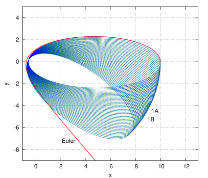
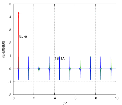
Figure 1: (Color online) First order algorithms 1A, 1B and Euler at ${\Delta t}=0.1$ Left: orbital trajectory; Right: normalized energy error as a function of $t$ in unit of the period $P$ of the exact orbit. See text for details.

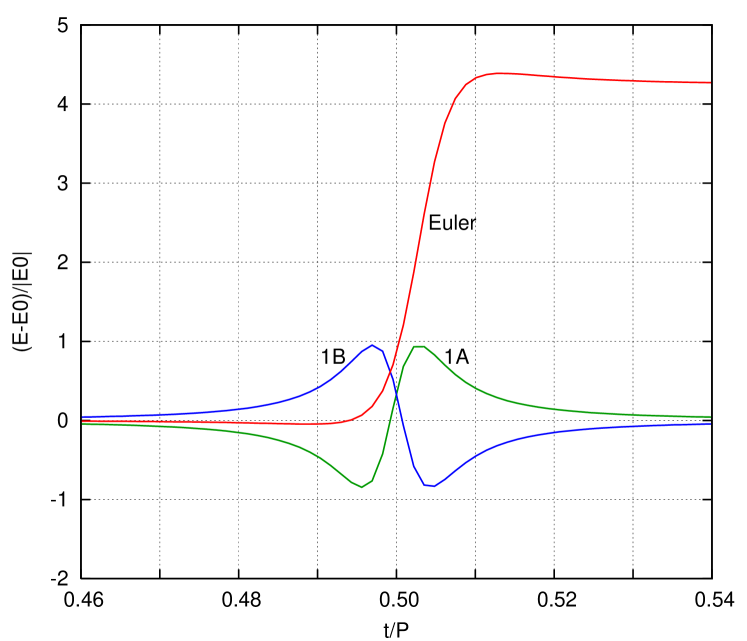
Figure 2: (Color online) Fractional energy errors of three first-order algorithms at midperiod.

To see how these algorithms actually perform, we solve the dimensionless two dimensional Kepler problem defined by

$$H=\frac{1}{2}{\bf p}^{2}-\frac{1}{|{\bf r}|},$$

with initial condition ${\bf r}=(10,0)$ and ${\bf p}=(0,0.1)$ at ${\Delta t}=0.1$. In Fig.1, we show the resulting trajectories and energy errors for $\approx 40$ periods. Because ${\Delta t}$ has been deliberately chosen to be large, the orbits generated by 1A and 1B do not close; they just precess. This precession of the Keplerian orbit is a common feature of CT, corresponding to perturbing the original Hamiltonian by the algorithm’s error terms defined in the next Section. (This precession is similar to Mercury’s perihelion advance due to the perturbation of general relativity.) Since 1A and 1B are very similar when iterated, their orbits, green and blue respectively, overlapped to yield a turquoise trajectory. By contrast, Euler can only complete half a orbit before the trajectory is ejected to infinity. On the right of Fig.1 are the fractional energy errors of each algorithm. For 1A and 1B, the energy errors only spike (but at nearly 100% !) periodically at midperiod. In the next Section, we will explain why the trajectory remained fairly intact despite such huge energy errors. In Fig.2, we zoom in at midperiod to resolve the fine structures. It shows clearly that 1A and 1B have equal and opposite energy errors.

IV Poissonian mechanics and the algebraization of algorithms

While it is easy to use (29) and (31) to produce first-order algorithms, it is not obvious how one can generalize either to obtain higher-order, more accurate methods. For this, we turn to the Poissonian formulation mechanics in terms of Poisson brackets.

For any dynamical variable $W(q_{i},p_{i})$, its evolution through the evolution of $q_{i}(t)$ and $p_{i}(t)$ is just

$$\frac{d}{dt}W(q_{i},p_{i})= \sum_{i=1}^{n}\Bigl{(}{{\partial W}\over{\partial q_{i}}}{{\partial q_{i}}\over{\partial t}}+{{\partial W}\over{\partial p_{i}}}{{\partial p_{i}}\over{\partial t}}\Bigr{)},$$

$$= \sum_{i=1}^{n}\Bigl{(}{{\partial W}\over{\partial q_{i}}}{{\partial H}\over{\partial p_{i}}}-{{\partial W}\over{\partial p_{i}}}{{\partial H}\over{\partial q_{i}}}\Bigr{)}\equiv\{W,H\},$$ (33)

where Hamilton’s equations (25) have been used to obtain the second line. The last equality defines the Poisson bracket of $W$ and $H$. We shall refer to this as Poisson’s equation-of-motion. This equation now gives us an alternatively way of derving canonical transformations. Let us rewrite (33) as

$${{dW}\over{dt}}=\{W,H\}=\hat{H}W,$$ (34)

and regard the Poisson bracket $\{W,H\}$ as defining an operator $\hat{H}$ acting on $W$. Clearly then,

$$\hat{H}=\sum_{i=1}^{n}\Bigl{(}{{\partial H}\over{\partial p_{i}}}{{\partial}\over{\partial q_{i}}}-{{\partial H}\over{\partial q_{i}}}{{\partial}\over{\partial p_{i}}}\Bigr{)}.$$

For the standard Hamiltonian (24), this operator is just

$$\hat{H}=\sum_{i=1}^{n}\Bigl{(}{{p_{i}}\over{m}}{{\partial}\over{\partial q_{i}}}+F_{i}{{\partial}\over{\partial p_{i}}}\Bigr{)},$$

which we can write it compactly as

$$\hat{H} = \hat{T}+\hat{V}$$ (35)

$$= {\bf v}\cdot\frac{\partial}{\partial{\bf q}}+{\bf a}({\bf q})\cdot\frac{\partial}{\partial{\bf v}},$$

with ${\bf v}\equiv{\bf p}/m$ and ${\bf a}\equiv-(\partial V/\partial{\bf q})/m$. We’ll just refer to $\hat{H}$, $\hat{T}$, and $\hat{V}$, as the classical Hamiltonian, kinetic energy and potential energy operators respectively.

For $H$ not explicitly dependent on time, (34) can be integrated to obtain the formal operator solution

$$W(q_{i},p_{i},t)={\rm e}^{t\hat{H}}W(q_{i},p_{i},0).$$ (36)

Let’s pause here to appreciate this remarkable Poissonian achievement. In the Newtonian, Lagrangian or Hamiltonian formulation, only the equations-of-motion are given, and one must solve them still. Here, in the Poissonian formulation, the solution (36) is already given, there is nothing more to solve! To see this, let’s consider the harmonic oscillator case with ${\bf a}({\bf q})=-{\omega}^{2}{\bf q}$ and apply (36) to ${\bf q}(t)$ and ${\bf v}(t)$:

$$\left(\begin{array}[]{c}{\bf q}(t)\\ {\bf v}(t)\end{array}\right) = {\rm e}^{t{\hat{H}}}\left(\begin{array}[]{c}{\bf q}\\ {\bf v}\end{array}\right)$$ (41)

$$= (1+t{\hat{H}}+\frac{1}{2}t^{2}{\hat{H}}^{2}+\frac{1}{3!}t^{3}{\hat{H}}^{3}+\frac{1}{4!}t^{4}{\hat{H}}^{4}+\cdots)\left(\begin{array}[]{c}{\bf q}\\ {\bf v}\end{array}\right)$$ (44)

From (35), we see that

$${\hat{H}}{\bf q}={\bf v},\quad{\hat{H}}^{2}{\bf q}=-{\omega}^{2}{\bf q},\quad{\hat{H}}^{3}{\bf q}=-{\omega}^{2}{\bf v},\quad{\hat{H}}^{4}{\bf q}={\omega}^{4}{\bf q}\quad\cdots$$

and therefore

$$\left(\begin{array}[]{c}{\bf q}(t)\\ {\bf v}(t)\end{array}\right) = \left(\begin{array}[]{c}{\bf q}+t{\bf v}-\frac{1}{2}t^{2}{\omega}^{2}{\bf q}-\frac{1}{3!}t^{3}{\omega}^{2}{\bf v}+\frac{1}{4!}t^{4}{\omega}^{4}{\bf q}+\cdots\\ \ \ {\bf v}-t{\omega}^{2}{\bf q}-\frac{1}{2}t^{2}{\omega}^{2}{\bf v}+\frac{1}{3!}t^{3}{\omega}^{4}{\bf q}+\frac{1}{4!}t^{4}{\omega}^{4}{\bf v}+\cdots\end{array}\right)$$ (49)

$$= \left(\begin{array}[]{c}\ \ \ \cos({\omega}t){\bf q}+{\omega}^{-1}{\sin({\omega}t)}{\bf v}\\ -{{\omega}}\,{\sin({\omega}t)}{\bf q}+\cos({\omega}t){\bf v}\end{array}\right)$$ (52)

which are the exact solutions with ${\bf q}={\bf q}(0)$ and ${\bf v}={\bf v}(0)$. Of course, when ${\bf a}({\bf q})$ is not linear in ${\bf q}$, it is generally not possible to sum the infinite series. However, we do have exact, closed forms for

$${\rm e}^{{\Delta t}{\hat{T}}}\left(\begin{array}[]{c}{\bf q}\\ {\bf v}\end{array}\right) = (1+{\Delta t}{\bf v}\cdot\partial_{\bf q}+\frac{1}{2}{\Delta t}^{2}({\bf v}\cdot\partial_{\bf q})^{2}+\cdots)\left(\begin{array}[]{c}{\bf q}\\ {\bf v}\end{array}\right)$$ (57)

$$= \left(\begin{array}[]{c}{\bf q}+{\Delta t}{\bf v}\\ {\bf v}\end{array}\right),$$ (60)

and

$${\rm e}^{{\Delta t}{\hat{V}}}\left(\begin{array}[]{c}{\bf q}\\ {\bf v}\end{array}\right) = \left(\begin{array}[]{c}{\bf q}\\ {\bf v}+{\Delta t}{\bf a}({\bf q})\end{array}\right).$$ (65)

Therefore, this suggests that one should regard the classical evolution operator ${\rm e}^{t{\hat{H}}}$ in (36) as $[{\rm e}^{{\Delta t}({\hat{T}}+{\hat{V}})}]^{n}$, and approximate the short-time evolution operator ${\rm e}^{{\Delta t}({\hat{T}}+{\hat{V}})}$ in terms of ${\rm e}^{{\Delta t}{\hat{T}}}$ and ${\rm e}^{{\Delta t}{\hat{V}}}$. Recalling the well-known Baker-Campell-Hausdorff formula,mil72

$${\rm e}^{A}{\rm e}^{B}={\rm exp}\left[A+B+{1\over 2}[A,B]+{1\over{12}}[A,[A,B]]+{1\over{12}}[B,[B,A]]+\cdots\right]$$

where $[A,B]\equiv AB-BA$, one immediately sees that

$${\cal T}_{1A}({\Delta t})\equiv{\rm e}^{{\Delta t}\hat{V}}{\rm e}^{{\Delta t}\hat{T}}={\rm e}^{{\Delta t}{\hat{H}}_{1A}}$$ (66)

with

$${\hat{H}}_{1A}={\hat{H}}+{1\over 2}{\Delta t}[{\hat{V}},{\hat{T}}]+{1\over{12}}{\Delta t}^{2}([{\hat{V}},[{\hat{V}},{\hat{T}}]]+[{\hat{T}},[{\hat{T}},{\hat{V}}]])\cdots.$$ (67)

Therefore when the right most term in (66) is expanded, its first order ${\Delta t}$ term (for the trajectory) is correct. At the same time, (67) shows that ${\hat{H}}_{1A}$, which is the exact Hamiltonian operator for ${\rm e}^{{\Delta t}\hat{V}}{\rm e}^{{\Delta t}\hat{T}}$, has a first-order ${\Delta t}$ error term as compared to the original Hamiltonian operator ${\hat{H}}$. The effect of ${\cal T}_{1A}$ is then

$${\rm e}^{{\Delta t}{\hat{V}}}{\rm e}^{{\Delta t}{\hat{T}}}\left(\begin{array}[]{c}{\bf q}\\ {\bf v}\end{array}\right) = {\rm e}^{{\Delta t}{\hat{V}}}\left(\begin{array}[]{c}{\bf q}+{\Delta t}{\bf v}\\ \ {\bf v}\end{array}\right)$$ (72)

$$= \left(\begin{array}[]{c}{\bf q}+{\Delta t}({\bf v}+{\Delta t}{\bf a}({\bf q}))\\ {\bf v}+{\Delta t}{\bf a}({\bf q})\end{array}\right).$$ (75)

Again, with ${\bf q}={\bf q}_{0}$, ${\bf v}={\bf v}_{0}$, and the last numbered values as the updated values, the above corresponds to the updating

$${\bf v}_{1} = {\bf v}_{0}+{\Delta t}{\bf a}_{0}$$

$${\bf q}_{1} = {\bf q}_{0}+{\Delta t}{\bf v}_{1},$$ (76)

which is the previously derived algorithm 1A. Note that the operators are applied from right to left as indicated, but the last applied operator gives the first updating of the variable, and the dynamical variables are updated in the reversed order according to the operators from left to right.

Similarily, the approximation

$${\cal T}_{1B}({\Delta t})\equiv{\rm e}^{{\Delta t}\hat{T}}{\rm e}^{{\Delta t}\hat{V}}={\rm e}^{{\Delta t}{\hat{H}}_{1B}}$$ (77)

with

$${\hat{H}}_{1B}={\hat{H}}+{1\over 2}{\Delta t}[{\hat{T}},{\hat{V}}]+{1\over{12}}{\Delta t}^{2}([{\hat{T}},[{\hat{T}},{\hat{V}}]]+[{\hat{V}},[{\hat{V}},{\hat{T}}]])\cdots.$$ (78)

gives

$${\rm e}^{{\Delta t}{\hat{T}}}{\rm e}^{{\Delta t}{\hat{V}}}\left(\begin{array}[]{c}{\bf q}\\ {\bf v}\end{array}\right)={\rm e}^{{\Delta t}{\hat{T}}}\left(\begin{array}[]{c}{\bf q}\\ {\bf v}+{\Delta t}{\bf a}({\bf q})\end{array}\right) = \left(\begin{array}[]{c}{\bf q}+{\Delta t}{\bf v}\\ {\bf v}+{\Delta t}{\bf a}({\bf q}+{\Delta t}{\bf v})\end{array}\right).$$ (85)

corresponds to the updating

$${\bf q}_{1}={\bf q}_{0}+{\Delta t}{\bf v}_{0}$$

$${\bf v}_{1}={\bf v}_{0}+{\Delta t}{\bf a}_{1},$$ (86)

where ${\bf a}_{1}\equiv{\bf a}({\bf q}_{1})$, which is algorithm 1B.

This way of deriving these two algorithms makes it very clear that the algorithms are sequential because the operators are applied sequentially, with each operator only acting on one dynamical variable at a time. More importantly, from (66) and (67), the trajectory produced by 1A is exact for the modified Hamiltonian operator ${\hat{H}}_{1A}$, which approaches the original ${\hat{H}}$ only as ${\Delta t}\rightarrow 0$. To find the modified Hamiltonian function $H_{1A}$ corresponding to ${\hat{H}}_{1A}$, we recall that ${\hat{H}}W=\{W,H\}$, and therefore

$$[{\hat{T}},{\hat{V}}]\,\,W = ({\hat{T}}{\hat{V}}-{\hat{V}}{\hat{T}})W={\hat{T}}\{W,V\}-{\hat{V}}\{W,T\}\,,$$ (87)

$$= \{\{W,V\},T\}-\{\{W,T\},V\}\,=\{W,\{V,T\}\}\,,$$

where the last equality follows from the Jacobi identity

$$\{\{W,V\},T\}+\{\{T,W\},V\}+\{\{V,T\},W\}=0\,.$$

From (87) we see that the function corresponding to $[{\hat{T}},{\hat{V}}]$ is $\{V,T\}=-\{T,V\}$, and that for the separable Hamiltonian (24)

$$\{T,V\}=\sum_{i=1}^{n}-\frac{{\partial}T}{{\partial}p_{i}}\frac{{\partial}V}{{\partial}q_{i}}={\bf v}\cdot{\bf F},$$

and therefore

$$H_{1A}=H+\frac{1}{2}{\Delta t}{\bf v}\cdot{\bf F}+\cdots\quad{\rm and}\quad H_{1B}=H-\frac{1}{2}{\Delta t}{\bf v}\cdot{\bf F}+\cdots$$ (88)

These modified Hamiltonians for algorithms 1A and 1B then explain the observations in Fig.2: 1) The energy errors are opposite in sign. 2) Since $|{\bf F}|\approx 1/r^{2}$ and $|{\bf v}|\approx 1/r$, the energy errors are nearly zero far from the force center. 3) Since at the pericenter ${\bf v}\cdot{\bf F}=0$, the first order energy errors cross zero at midperiod. The fact that they don’t in Fig.2 simply means that the remaining higher order error terms in (88) do not vanish at the pericenter. For example,

$$[{\hat{V}},[{\hat{T}},{\hat{V}}]]\longrightarrow\{[{\hat{T}},{\hat{V}}],V\}\longrightarrow\{\{V,T\},V\}\longrightarrow\{V,\{T,V\}\},$$

and

$$\{V,\{T,V\}\}=\sum_{i=1}^{n}\frac{{\partial}V}{{\partial}q_{i}}\frac{{\partial}\{T,V\}}{{\partial}p_{i}}=-\frac{{\bf F}\cdot{\bf F}}{m},$$ (89)

which peaks strongly near the force center as $1/|{\bf r}|^{4}$. 4) The error terms in (88), spoil the the exact inverse-square nature of the force, and therefore by Bertrand’s theorem,ber73 ; chin15 the orbit cannot close, resulting in precessions as seen in Fig.1. 5) Because of this precession, the energy errors are periodic at midperiod. We can explain these observations in details because a symplectic integrator remains governed by a Hamiltonian, though modified. Very little can be say about the behavor of non-symplectic algorithms such as Euler, except that they are ultimately unstable because they are not bound by a Hamiltonian.

In general then, one can seek to approximate ${\rm e}^{{\Delta t}({\hat{T}}+{\hat{V}})}$ by a product of ${\rm e}^{{\Delta t}{\hat{T}}}$ and ${\rm e}^{{\Delta t}{\hat{V}}}$ in the form of

$${\rm e}^{{\Delta t}({\hat{T}}+{\hat{V}})}=\prod_{i=1}^{n}{\rm e}^{c_{i}{\Delta t}{\hat{T}}}{\rm e}^{d_{i}{\Delta t}{\hat{V}}},$$ (90)

with real coefficients $\{c_{i},d_{i}\}$ determined to match ${\rm e}^{{\Delta t}({\hat{T}}+{\hat{V}})}$ to any order in ${\Delta t}$. Since a product of operators represent a sequential updating of one dynamical variable at a time with Jacobians (21), the resulting algorithm is guranteed to have $\det M=1$. Also, since each operator is a canonical transformation, the entire sequence is also a canonical transformation. Thus we now have a method of generating arbitrarily accurate canonical transformations. Moreover, this process of decomposition, of approximating ${\rm e}^{{\Delta t}({\hat{T}}+{\hat{V}})}$ by a product of ${\rm e}^{c_{i}{\Delta t}{\hat{T}}}$ and ${\rm e}^{d_{i}{\Delta t}{\hat{V}}}$, reduces the original problem of Taylor series analysis into an algebraic problem of operator factorization. Finally, this product approximation of ${\rm e}^{{\Delta t}({\hat{T}}+{\hat{V}})}$, for any two operators ${\hat{T}}$ and ${\hat{V}}$, can be applied to any other physical evolution equation.

Similar to the Hamiltonian function, one can define an operator $\hat{S}$ corresponding to any dynamical function $S(q_{i},p_{i})$ via the Poisson bracket $\{W,S\}=\hat{S}W$. It is then easy to provedep69 ; boc98 that the transformation generated by ${\rm e}^{\epsilon\hat{S}}$, for any $S(q_{i},p_{i})$, is also canonical. Such an operator $\hat{S}$ is called a Lie operator and the series evaluation of ${\rm e}^{\epsilon\hat{S}}$ as the Lie seriesdep69 method. These seminal ideas from celestial mechanicsdep69 ; boc98 and accelerator physics, dra76 ; fr90 ; for06 forged the modern development of symplectic integrators.ner87 ; yos93 (In this Section, it is also imperative that we use an intuitive and non-intimidating notation to denote Lie operators such as $\hat{H}$ or $\hat{S}$. The direct usegol80 of $\{\cdot,S\}$ leads to unwieldy expression for powers of $\hat{S}^{n}$ as $...\{\{\{\{\cdot,S\},S\},S\},S\}..$. The old time typographical notationdra76 ; fr90 of “:$S$:” is unfamiliar to modern readers. The use of “$L_{S}$” dep69 ; boc98 or “$D_{S}$” don05 is redundant, with the symbol “$L$” or “$D$” serving no purpose. In this work, we eschew these three conventions and follow a practice already familiar to students (from quantum mechanics) by denoting a Lie operator with a “caret” over its defining function, $\hat{S}$. Also, it is essential to define $\hat{H}=\{\cdot,H\}$, and not $\hat{H}=\{H,\cdot\}$, otherwise one gets a confusing negative sign for moving forward in time.)

V Time-reversibility and second-order algorithms

The two first-order algorithms derived so far, despite being cannonical, are not time-reversible, that is, unlike the exact trajectory, they cannot retrace their steps back to the original starting point when run backward in time. This point is not obvious when they were first derived from generating functions. In the operator formulation, this is now transparent because

$${\cal T}_{1A}(-{\Delta t}){\cal T}_{1A}({\Delta t})={\rm e}^{-{\Delta t}{\hat{V}}}{\rm e}^{-{\Delta t}{\hat{T}}}{\rm e}^{{\Delta t}{\hat{V}}}{\rm e}^{{\Delta t}{\hat{T}}}\neq 1.$$

Similarly for $1B$. This means that these two first-order algorithms may yield trajectories qualitatively different from the exact solution. For example, the phase trajectory for the harmonic oscillator with $H=(p^{2}+q^{2})/2$ (${\omega}=1$) should just be a circle. However, the modified Hamiltonians for 1A and 1B from (88) are

$$H_{1A}=\frac{1}{2}(p^{2}+q^{2}-{\Delta t}pq)=\frac{1}{2}\left(\frac{u^{2}}{(1-{\Delta t}/2)^{-1}}+\frac{v^{2}}{(1+{\Delta t}/2)^{-1}}\right),$$

$$H_{1B}=\frac{1}{2}(p^{2}+q^{2}+{\Delta t}pq)=\frac{1}{2}\left(\frac{u^{2}}{(1+{\Delta t}/2)^{-1}}+\frac{v^{2}}{(1-{\Delta t}/2)^{-1}}\right),$$

with $u=(p+q)/\sqrt{2}$ and $v=(p-q)/\sqrt{2}$. For $|{\Delta t}|<2$, these are now ellipseslar83 ; don05 with semi-major axes tilted at $\pm 45^{\circ}$. This $45^{\circ}$ tilt is uncharacteristic of the exact trajectory.

This shortcoming can be easily fixed by just cancatenating $1A$ and $1B$ together, giving

$${\cal T}_{2A}({\Delta t})={\cal T}_{1A}({\Delta t}/2){\cal T}_{1B}({\Delta t}/2)={\rm e}^{{\Delta t}{\hat{V}}/2}{\rm e}^{{\Delta t}{\hat{T}}}{\rm e}^{{\Delta t}{\hat{V}}/2}={\rm e}^{{\Delta t}{\hat{H}}_{2A}({\Delta t})},$$ (91)

with left-right symmetric operators, guaranteeing time-reversibility:

$${\cal T}_{2A}(-{\Delta t}){\cal T}_{2A}({\Delta t})={\rm e}^{-{\Delta t}{\hat{V}}/2}{\rm e}^{-{\Delta t}{\hat{T}}}{\rm e}^{-{\Delta t}{\hat{V}}/2}{\rm e}^{{\Delta t}{\hat{V}}/2}{\rm e}^{{\Delta t}{\hat{T}}}{\rm e}^{{\Delta t}{\hat{V}}/2}=1.$$ (92)

This means that the algorithm’s Hamiltonian operator must be of the form

$${\Delta t}{\hat{H}}_{2A}({\Delta t})={\Delta t}({\hat{H}}+{\Delta t}^{2}\hat{E}_{2}+{\Delta t}^{4}\hat{E}_{4}+\cdots),$$ (93)

with only even-order error operators $\hat{E}_{2},\hat{E}_{4},$ etc., otherwise, if ${\hat{H}}_{2A}({\Delta t})$ has any odd-order error term, then ${\Delta t}{\hat{H}}_{2A}({\Delta t})$ would have a term even in ${\Delta t}$ and ${\rm e}^{-{\Delta t}{\hat{H}}_{2A}(-{\Delta t})}{\rm e}^{{\Delta t}{\hat{H}}_{2A}({\Delta t})}\neq 1,$ contradicting (92). Thus any decomposition with left-right symmetric operators must yield an even-order algorithm, of at least second-order.

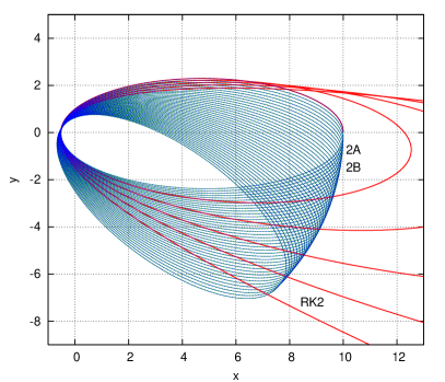
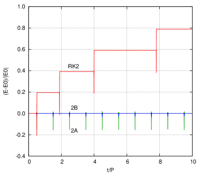
Figure 3: (Color online) Trajectory and energy errors similar to Fig.1 for three second-order algorithms 2A, 2B and RK2 at ${\Delta t}=0.1$ .

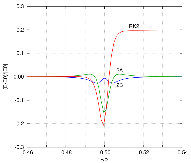
Figure 4: (Color online) Energy errors at midperiod for the three second-order algorithms of Fig.3.

The action of ${\cal T}_{2A}({\Delta t})$

$${\rm e}^{{\Delta t}{\hat{V}}/2}{\rm e}^{{\Delta t}{\hat{T}}}{\rm e}^{{\Delta t}{\hat{V}}/2}\left(\begin{array}[]{c}{\bf q}\\ {\bf v}\end{array}\right) = {\rm e}^{{\Delta t}{\hat{V}}/2}\left(\begin{array}[]{c}{\bf q}+{\Delta t}{\bf v}\\ {\bf v}+\frac{1}{2}{\Delta t}{\bf a}({\bf q}+{\Delta t}{\bf v})\end{array}\right)$$ (98)

$$= \left(\begin{array}[]{c}{\bf q}+{\Delta t}\Bigl{[}{\bf v}+\frac{{\Delta t}}{2}{\bf a}({\bf q})\Bigr{]}\\ \Bigl{[}{\bf v}+\frac{{\Delta t}}{2}{\bf a}({\bf q})\Bigr{]}+\frac{1}{2}{\Delta t}{\bf a}({\bf q}+{\Delta t}\Bigl{[}{\bf v}+\frac{{\Delta t}}{2}{\bf a}({\bf q})\Bigr{]}),\end{array}\right),$$ (101)

yields the second-order algorithm 2A:

$${\bf v}_{1} = {\bf v}_{0}+\frac{1}{2}{\Delta t}{\bf a}_{0},$$

$${\bf q}_{1} = {\bf q}_{0}+{\Delta t}{\bf v}_{1},$$

$${\bf v}_{2} = {\bf v}_{1}+\frac{1}{2}{\Delta t}{\bf a}_{1}.$$ (102)

Similarly, cancatenating 1B and 1A together gives

$${\cal T}_{2B}({\Delta t})={\cal T}_{1B}({\Delta t}/2){\cal T}_{1A}({\Delta t}/2)={\rm e}^{{\Delta t}{\hat{T}}/2}{\rm e}^{{\Delta t}{\hat{V}}}{\rm e}^{{\Delta t}{\hat{T}}/2}={\rm e}^{{\Delta t}{\hat{H}}_{2B}({\Delta t})},$$ (103)

yielding the corresponding 2B algorithm

$${\bf q}_{1} = {\bf q}_{0}+\frac{1}{2}{\Delta t}{\bf v}_{0},$$

$${\bf v}_{1} = {\bf v}_{0}+{\Delta t}{\bf a}_{1},$$

$${\bf q}_{2} = {\bf q}_{1}+\frac{1}{2}{\Delta t}{\bf v}_{1}.$$ (104)

These two symplectic schemes, when solving the harmonic oscillator, do not have any cross term $\propto pq$ in their modified Hamiltonians, and therefore will not have any extraneous $45^{\circ}$ tilts in their phase trajectories.

The sequential steps of algorithms 2A and 2B can be directly translated into programming lines and there is no need to combine them. However, for comparison, steps in 2A can be combined to give

$${\bf q}_{1} = {\bf q}_{0}+{\Delta t}{\bf v}_{0}+\frac{1}{2}{\Delta t}^{2}{\bf a}_{0},$$ (105)

$${\bf v}_{2} = {\bf v}_{0}+\frac{1}{2}{\Delta t}({\bf a}_{0}+{\bf a}_{1}),$$ (106)

which is just the velocity-Verletgou07 algorithm, or Stanley’s second-order Taylor approximation, STA.sta84 Note that the acceleration computed at the end, ${\bf a}_{1}$, can be reused as ${\bf a}_{0}$ at the start of the next iteration. Thus for both algorithms, only one force-evaluation is needed per iteration. Algorithm 2B is referred to as the position-Verletgou07 algorithm, which corresponds to Stanley’s STA^′ algorithm. These two canonical second-order algorithms were known before Stanley’s time, but were unrecognized as symplectic integrators among a host of other similarly looking algorithms.sta84

We compare the working of these two second-order algorithm in Fig.3. Not suprisingly, the lengthy iteration of 2A and 2B yielded trajectories similar to those of 1A and 2B. Note however, that their periodic energy errors are now much smaller. As shown in Fig.4, the maximum energy errors of 2A and 2B are only $\approx 15\%$ and $\approx 3\%$ respectively. Since the expected errors are on the order of O(${\Delta t}^{2}$), 2B’s error is entirely reasonable, while that of 2A is larger than expected. Nevertheless, these errors are more commensurate with their well-behave trajectories, similar to those of 1A and 1B. Thus the trajectories of 1A and 1B are nearly second-order; only that their energy errors do not reflect this. Plotted also are results for a Runge-Kutta type second-order algorithm RK2 derived in Section VII. Its trajectory manages to return to the force center a few times, but was eventually ejected to infinity. As we will see, it is characteristic of Runge-Kutta algorithms that the magnitude of their energy errors is non-periodic and ever increasing with each orbit.

VI Higher order symplectic algorithms

We have derived two second-order algorithms effortlessly without doing any Taylor expansions. We will now show, with equal ease, how to derive higher order symplectic algorithms. From (93), one has (where ${\cal T}_{2}$ denotes either ${\cal T}_{2A}$ or ${\cal T}_{2B}$)

$${\cal T}_{2}({\Delta t})=\exp({\Delta t}\hat{H}+{\Delta t}^{3}\hat{E}_{2}+{\Delta t}^{5}\hat{E}_{4}+\cdots),$$ (107)

with only odd powers of ${\Delta t}$ in the exponent. If one were able to get rid of the ${\Delta t}^{3}$ term, one would have a fourth-order algorithm. Consider then a triple product of ${\cal T}_{2}$ with a negative time step $-s{\epsilon}$ at the middle:

$${\cal T}_{2}(\epsilon){\cal T}_{2}(-s\epsilon){\cal T}_{2}(\epsilon)={\rm exp}[(2-s)\epsilon\hat{H}+(2-s^{3})\epsilon^{3}\hat{E}_{2}+O(\epsilon^{5})].$$ (108)

This algorithm evolves the system forward for time $\epsilon$, backward for time $s\epsilon$ and forward again for time $\epsilon$. Since it is manifestly left-right symmetric, and hence time-reversible, its exponent must consist of terms with only odd powers of $\epsilon$. Moreover, its leading ${\epsilon}^{3}$ term can only be due to the sum of ${\epsilon}^{3}$ terms from each constituent algorithm, without any commutator terms. This is because any single-commutator of ${\epsilon}\hat{H}$, ${\epsilon}^{3}\hat{E}_{2}$, etc., would be even in ${\epsilon}$ and hence excluded. Any double-commutator would have a minimum of two ${\epsilon}\hat{H}$ and one ${\epsilon}^{3}\hat{E}_{2}$, which is already fifth order in ${\epsilon}$.

To obtain a fourth-order algorithm, it is only necessary to eliminate the ${\epsilon}^{3}$ error term in (108) by choosing

$$s=2\,^{1/3}$$

and scale $\epsilon$ back to the standard step size by setting ${\Delta t}=(2-s)\epsilon$,

$${\cal T}_{4}({\Delta t})\equiv{\cal T}_{2}\Bigl{(}{{\Delta t}\over{2-s}}\Bigr{)}{\cal T}_{2}\Bigl{(}{-s\,{\Delta t}\over{2-s}}\Bigr{)}{\cal T}_{2}\Bigl{(}{{\Delta t}\over{2-s}}\Bigr{)}={\rm exp}[\,{\Delta t}\hat{H}+O({\Delta t}^{5})].$$ (109)

This fourth-order algorithm only requires 3 force-evaluations.

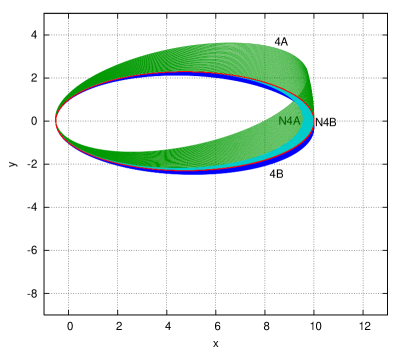
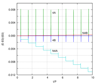
Figure 5: (Color online) Trajectory and energy errors similar to Fig.1 for four fourth-order algorithms 4A(green), 4B(blue), N4A(blue-green) and N4B(a red closed ellipse) at ${\Delta t}=0.1$

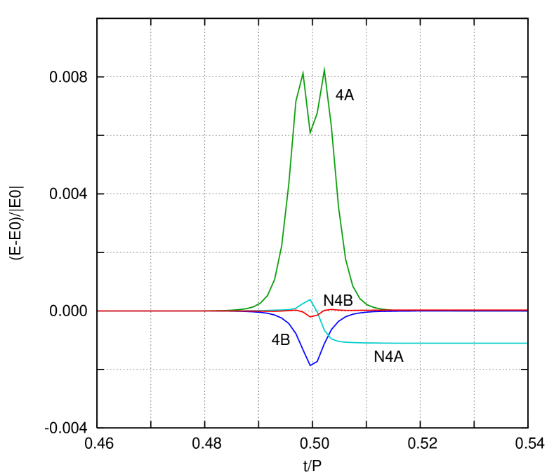
Figure 6: (Color online) Energy errors at midperiod for four fourth-order algorithms of Fig.5.

The derivation of the first fourth-order SI in the late 1980’s initiated the modern development of symplectic integrators. According to Forest,for06 the first fourth-order SI was obtained by Ruth in 1985 by numerically solving equations with hundreds of terms. However, their lengthy derivation of the algorithm involving a complicated cube root was not published jointly until 1990.fr90 Around the same time, many groups, including Campostrini and Rossi,cam90 Suzuki,suz90 Yoshida,yos90 , Candy and Rozmouscan91 and Bandrauk and Shen,ban91 have independently arrived at the same algorithm, but it was Creutz and Gockschcre89 who managed to publish it in 1989. Here, we follow the simpler derivation of Ref.chin00, .

By letting ${\cal T}_{2}$ be either ${\cal T}_{2A}$ or ${\cal T}_{2B}$ in (109), one obtains fourth-order algorithms 4A and 4B respectively. Their trajectories for the same Keplerian orbit at ${\Delta t}=0.1$ are shown in Fig.5. The orbital precession is now much reduced and their periodic energy errors in Fig.6 are roughly ten times smaller than those of 2A and 2B. Notice that, just as the energy error of 2B is much smaller than 2A, 4B’s maximum energy error and orbital precession are much less than those of 4A. Also plotted are results for Runge-Kutta type Nyström algorithms N4A and N4B, which are derived in the next section.

Clearly, the triple-product construction can be repeated to generate arbitrary even-order algorithms. For example, a sixth-order algorithm can be obtained by taking

$${\cal T}_{6}\equiv{\cal T}_{4}\Bigl{(}{{\Delta t}\over{2-s}}\Bigr{)}{\cal T}_{4}\Bigl{(}{-s\,{\Delta t}\over{2-s}}\Bigr{)}{\cal T}_{4}\Bigl{(}{{\Delta t}\over{2-s}}\Bigr{)}.$$ (110)

and choosing $s=2^{1/5}$ to eliminate the fifth-order error term in ${\cal T}_{4}$. One can then cancatenates three ${\cal T}_{6}$ to give ${\cal T}_{8}$ by choosing $s=2^{1/7}$ etc.. Thus, without doing any tedious analysis, one can easily generate any even-order algorithms. The disadvantage of this class of schemes is that the the number of force-evaluation needed at order $2n$ grows exponentially as $3^{n-1}$. It is already uneconomical at order six, which required nine force-evaluations. As we will see in the next section, a sixth-order RKN algorithm only requires five force-evaluations. Moreover, as shown in Fig.5, even the better symplectic 4B algorithm seems inferior, in the short run, to N4B.

VII Higher-order Runge-Kutta-Nyström algorithms

Runge-Kutta type schemes generalize the Euler algorithm to higher order. For example, keeping the Taylor expansion to second-order, gives

$${\bf q}({\Delta t}) = {\bf q}(0)+{\Delta t}\dot{\bf q}(0)+\frac{1}{2}{\Delta t}^{2}\ddot{\bf q}(0)$$

$${\bf q}_{1} = {\bf q}_{0}+{\Delta t}{\bf v}_{0}+\frac{1}{2}{\Delta t}^{2}{\bf a}_{0}$$ (111)

and

$${\bf v}({\Delta t}) = {\bf v}(0)+{\Delta t}\dot{\bf v}(0)+\frac{1}{2}{\Delta t}^{2}\ddot{\bf v}(0)$$

$${\bf v}_{1} = {\bf v}_{0}+{\Delta t}{\bf a}_{0}+\frac{1}{2}{\Delta t}^{2}\dot{\bf a}_{0}={\bf v}_{0}+{\Delta t}({\bf a}_{0}+\frac{1}{2}{\Delta t}{\bf v}_{0}\cdot\nabla{\bf a}_{0})$$ (112)

$$= {\bf v}_{0}+{\Delta t}{\bf a}({\bf q}_{0}+\frac{1}{2}{\Delta t}{\bf v}_{0})+O({\Delta t}^{3})$$

$$= {\bf v}_{0}+\frac{1}{2}{\Delta t}[{\bf a}_{0}+{\bf a}({\bf q}_{0}+{\Delta t}{\bf v}_{0})]+O({\Delta t}^{3})$$ (113)

The idea is to replace higher order time-derivatives by evaluating the force at some intermediate positions. Both (112) and (113) are correct to ${\Delta t}^{2}$ and are acceptable implementation of this second-order Runge-Kutta algorithm (RK2). Both also require two evaluations of the force, which are inferior to only a single evaluation needed in 2A and 2B. If one chooses the implemention (113), then one can easily check that this RK2 is just the average of algorithms 1A and 1B, that is

$${\cal T}_{RK2}({\Delta t})=\frac{1}{2}({\rm e}^{{\Delta t}{\hat{T}}}{\rm e}^{{\Delta t}{\hat{V}}}+{\rm e}^{{\Delta t}{\hat{V}}}{\rm e}^{{\Delta t}{\hat{T}}}).$$

Thus Runge-Kutta type algorithms can also have an operator representation, except that they are no longer a single product as in (90). This automatically implies that they are no longer sequential and can’t have $\det M=1$. As shown in Fig.3, RK2’s energy error increases indefinitely with each period until total destablization.

The triplet construction of higher order symplectic algorithms is based on eliminating the errors (107) of ${\cal T}_{2}$, , via a product of ${\cal T}_{2}$’s. However, since

$${\cal T}_{2}^{k}({\Delta t}/k)=\exp({\Delta t}\hat{H}+k^{-2}{\Delta t}^{3}\hat{E}_{2}+k^{-4}{\Delta t}^{5}\hat{E}_{4}+\cdots),$$ (114)

these higher order errors can alternatively be eliminated by extrapolation. For example, a fourth-order algorithm can also be obtained by the combination

$${\cal T}_{4}({\Delta t})=\frac{1}{3}\Bigl{[}4{\cal T}_{2}^{2}\left(\frac{{\Delta t}}{2}\right)-{\cal T}_{2}({\Delta t})\Bigr{]},$$ (115)

where the factor 4 cancels the ${\Delta t}^{3}$ error term and the factor 3 restores the original Hamiltonian term ${\Delta t}H$. Because this is no longer a single product of operators, the algorithm is again no longer symplectic with $\det M=1$. Take ${\cal T}_{2}$ to be ${\cal T}_{2A}$, whose algorithmic form is given by (106), then ${\cal T}^{2}_{2A}({\Delta t}/2)$ corresponds to iterating that twice at half the step size:

$${\bf q}_{1}^{\prime} = {\bf q}_{0}+\frac{1}{2}{\Delta t}{\bf v}_{0}+\frac{1}{8}{\Delta t}^{2}{\bf a}_{0},$$ (116)

$${\bf v}_{2}^{\prime} = {\bf v}_{0}+\frac{1}{4}{\Delta t}({\bf a}_{0}+{\bf a}_{1^{\prime}}),$$

$${\bf q}_{2} = {\bf q}_{1}^{\prime}+\frac{1}{2}{\Delta t}{\bf v}^{\prime}_{2}+\frac{1}{8}{\Delta t}^{2}{\bf a}_{1^{\prime}},$$

$${\bf v}_{3} = {\bf v}_{2}^{\prime}+\frac{1}{4}{\Delta t}({\bf a}_{1^{\prime}}+{\bf a}_{2}).$$

The first two lines are just (106) at ${\Delta t}/2$, and the second two lines simply repeat that with ${\bf q}_{1}^{\prime}$ and ${\bf v}_{2}^{\prime}$ as initial values. Eliminating the intermediate values ${\bf q}_{1}^{\prime}$ and ${\bf v}_{2}^{\prime}$ gives

$${\bf q}_{2} = {\bf q}_{0}+{\Delta t}{\bf v}_{0}+\frac{1}{4}{\Delta t}^{2}({\bf a}_{0}+{\bf a}_{1^{\prime}}),$$ (117)

$${\bf v}_{3} = {\bf v}_{0}+\frac{1}{4}{\Delta t}({\bf a}_{0}+2{\bf a}_{1^{\prime}}+{\bf a}_{2}).$$

The combination (115) then gives

$${\bf q}({\Delta t}) = \frac{4}{3}{\bf q}_{2}-\frac{1}{3}{\bf q}_{1}={\bf q}_{0}+{\Delta t}\,{\bf v}_{0}+\frac{{\Delta t}^{2}}{6}\left({\bf a}_{0}+2{\bf a}_{1^{\prime}}\right),$$ (118)

$${\bf v}({\Delta t}) = \frac{4}{3}{\bf v}_{3}-\frac{1}{3}{\bf v}_{2}={\bf v}_{0}+\frac{{\Delta t}}{6}\left({\bf a}_{0}+4{\bf a}_{1^{\prime}}+2{\bf a}_{2}-{\bf a}_{1}\right).$$ (119)

This appears to required 4 force-evaluations at ${\bf q}_{0}$, ${\bf q}_{1}^{\prime}$ (116), ${\bf q}_{2}$ (117) and ${\bf q}_{1}$ (111). However, the force subtraction above can be combined:

$$2{\bf a}_{2}-{\bf a}_{1} = 2{\bf a}({\bf q}_{2})-{\bf a}({\bf q}_{1})=2{\bf a}({\bf q}_{1}+\delta{\bf q})-{\bf a}({\bf q}_{1})$$ (120)

$$= {\bf a}({\bf q}_{1})+2\delta{\bf q}\cdot\nabla{\bf a}({\bf q}_{1})+O(\delta{\bf q}^{2})={\bf a}({\bf q}_{1}+2\delta{\bf q})+O(\delta{\bf q}^{2})$$

$$= {\bf a}({\bf q}_{0}+{\Delta t}{\bf v}_{0}+\frac{1}{2}{\Delta t}^{2}{\bf a}_{1^{\prime}})+O({\Delta t}^{6}),$$

since

$$\delta{\bf q} = {\bf q}_{2}-{\bf q}_{1}=\frac{{\Delta t}^{2}}{4}({\bf a}_{1^{\prime}}-{\bf a}_{0})\approx O({\Delta t}^{3}).$$

Hence, correct to $O({\Delta t}^{4})$, the two force-evaluations $2{\bf a}_{2}-{\bf a}_{1}$ in (119) can be replaced by the single force-evaluation (120). The resulting algorithm, (118) and (119), then reproduces Nyström’s original fourth-order integrator with only three force evaluations.nys25 ; bat99 We denote this algorithm as N4A. Using ${\cal T}_{2B}$ in (115) yields the algorithm N4B. In Fig.5, we see that N4A’s orbit is not precessing, but is continually shrinking, reflecting its continued loss of energy after each period. N4B’s energy error is monotonically increasing after each period, and will eventually destablize after a long time. However, its increase in energy error is remarkable small in the short term (see Fig.6), maintaining a closed orbit even after 40 periods. (A clearer picture of N4B’s orbit is given in Fig.7 below.) Thus in the short term, algorithms 4A and 4B, despite being symplectic, are inferior to N4B. We will take up this issue in the next section.

The standard fourth-order Runge-Kutta (RK4) algorithm,wil92 capable of solving the a general position-, velocity- and time-dependent force with ${\bf a}({\bf q},{\bf v},t)$, requires four force-evaluations. When the force does not depend on v, Nyström type algorithms only need three force-evaulations. When applied to Kepler’s problem, RK4, despite having four force-evaluations, behaved very much like N4A, and was therefore not shown separately.

The extrapolation, or the multi-product expansion (115), can be generalized to arbitrary evenchin10 or oddchin11 orders with analytically known coefficients, for example:

$${\cal T}_{6}({\epsilon})=\frac{1}{24}{\cal T}_{2}({\Delta t})-\frac{16}{15}{\cal T}_{2}^{2}\left(\frac{{\Delta t}}{2}\right)+\frac{81}{40}{\cal T}_{2}^{3}\left(\frac{{\Delta t}}{3}\right),$$

$${\cal T}_{8}({\epsilon})=-\frac{1}{360}{\cal T}_{2}({\Delta t})+\frac{16}{45}{\cal T}_{2}^{2}\left(\frac{{\Delta t}}{2}\right)-\frac{729}{280}{\cal T}_{2}^{3}\left(\frac{{\Delta t}}{3}\right)+\frac{1024}{315}{\cal T}_{2}^{4}\left(\frac{{\Delta t}}{4}\right).$$

Subsitute in ${\cal T}_{2A}$ or ${\cal T}_{2B}$ would then yield RKN type algorithms.chin10 Algorithms of up to the 100th-order have been demonstrated in Ref.chin11, . Since each ${\cal T}_{2}$ (especially ${\cal T}_{2B}$) only requires a single force-evaluation, a $2n$-order algorithm above would require $1+2+\cdots+n=n(n+1)/2$ force evaluations. Thus at higher orders, RKN’s use force evaluations is only quadratic, rather than geometric, as in the case of SI. For order $p=3$ to 6, force subtractions can be combined similarly as in the fourth-order case for ${\cal T}_{2A}$ so that the number of force-evaluation is reduced to $p-1$. Most known RKN algorithmsbat99 up to order six can be derived in this manner.chin10 At order $p=7$, the number of force-evaluation is 7. At order $p>7$, the number of force-evaluation is greater the $p$. The distinction between symplectic and RKN algorithms can now be understood as corresponding to a single operator product or a sum of operator products.

VIII Forward time-step algorithms

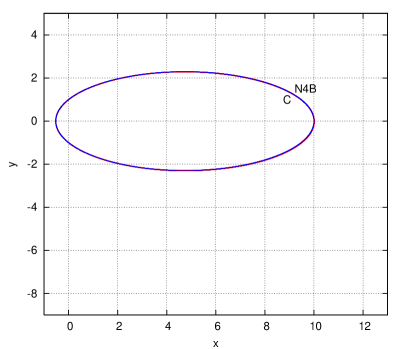
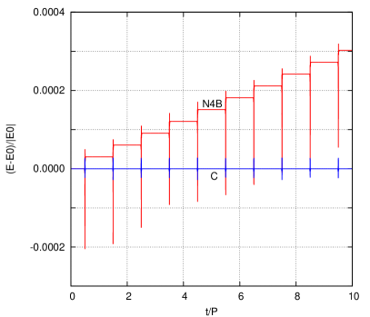
Figure 7: (Color online) Trajectory and energy errors similar to Fig.1 for fourth-order algorithms N4B (red) and C (blue) at ${\Delta t}=0.1$. The 40 orbits of both blended into a single purple orbit.

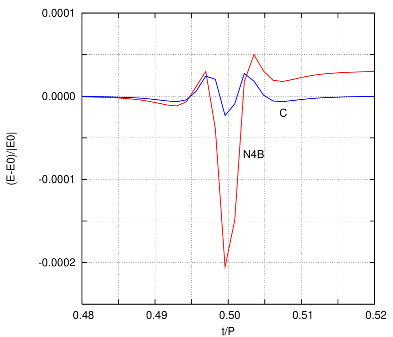
Figure 8: (Color online) Energy errors at midperiod for two fourth-order algorithms of Fig.7.

Soon after the discovery of the triplet construction (109), it was realizedcan91 that the resulting SI was not that superior to fourth-order RKN type algorithms in the short term, as shown in the last section. The problem can be traced to the large negative time-step in (109), which is $\approx-1.7{\Delta t}$. It then needs to cancel the two forward time step each at $\approx 1.35{\Delta t}$, to give back ${\Delta t}$. Clearly such a large cancellation is undesirable because evaluating ${\cal T}_{2}$ at time steps as large as $\approx 1.7{\Delta t}$ is less accurate. To avoid such a cancellation, one might dispense with the triplet construction (109) and seek to devise SI directly from a single operator product as in (90). Unfortunately, even with the general approach of (90), it is not possible to eliminate negative time steps (and therefore cancellations) beyond second order, i.e., beyond second order, $\{c_{i},d_{i}\}$ cannot all be positive. Formally, this result has been proved variously by Sheng,she89 Suzuki,suz91 Goldman and Kaper,gol96 Blandes and Casas,blanes05 and Chinchin06 . However, by repeated application of the BCH formula, one can showchin97 that,

$${\rm e}^{\frac{1}{3}{\Delta t}{\hat{T}}}{\rm e}^{\frac{3}{4}{\Delta t}{\hat{V}}}{\rm e}^{\frac{2}{3}{\Delta t}{\hat{T}}}{\rm e}^{\frac{1}{4}{\Delta t}{\hat{V}}} = {\rm e}^{{\Delta t}({\hat{T}}+{\hat{V}})-\frac{1}{48}{\Delta t}^{3}[{\hat{V}},[{\hat{T}},{\hat{V}}]]+O({\Delta t}^{4})},$$

$${\rm e}^{\frac{1}{3}{\Delta t}{\hat{T}}}{\rm e}^{\frac{3}{4}{\Delta t}{\hat{V}}}{\rm e}^{\frac{2}{3}{\Delta t}{\hat{T}}}{\rm e}^{\frac{1}{4}{\Delta t}{\hat{V}}}{\rm e}^{\frac{1}{48}{\Delta t}^{3}[{\hat{V}},[{\hat{T}},{\hat{V}}]]} = {\rm e}^{{\Delta t}({\hat{T}}+{\hat{V}})+O({\Delta t}^{4})}.$$

$${\rm e}^{\frac{1}{3}{\Delta t}{\hat{T}}}{\rm e}^{\frac{3}{4}{\Delta t}{\hat{V}}}{\rm e}^{\frac{2}{3}{\Delta t}{\hat{T}}}{\rm e}^{\frac{1}{4}{\Delta t}{\hat{V}}+\frac{1}{48}{\Delta t}^{3}[{\hat{V}},[{\hat{T}},{\hat{V}}]]} = {\rm e}^{{\Delta t}({\hat{T}}+{\hat{V}})+O({\Delta t}^{4})}.$$ (121)

Since

$$[{\hat{V}},[{\hat{T}},{\hat{V}}]]=2a_{j}\frac{\partial a_{i}}{\partial q_{j}}\frac{\partial}{\partial v_{i}}=\nabla_{i}(|{\bf a}|^{2})\frac{\partial}{\partial v_{i}},$$

is just an additional force term, it can be combined together with ${\hat{V}}=a_{i}(\partial/\partial v_{i})$. (Note that $\partial a_{i}/\partial q_{j}\propto\partial V/(\partial q_{i}\partial q_{j})=\partial a_{j}/\partial q_{i})$. This additional force is the same as that derived from the potential term corresponding to $[{\hat{V}},[{\hat{T}},{\hat{V}}]]$ given by (89). All the time-steps on the RHS of (121) are then positive. If one now symmetrized (121) to get rid of all the even order ${\Delta t}$ error terms, then one arrives at a fourth-order algorithm:

$${\cal T}_{C}({\Delta t})={\rm e}^{\frac{1}{6}{\Delta t}{\hat{T}}}{\rm e}^{\frac{3}{8}{\Delta t}{\hat{V}}}{\rm e}^{\frac{1}{3}{\Delta t}{\hat{T}}}{\rm e}^{\frac{1}{4}{\Delta t}({\hat{V}}+\frac{{\Delta t}^{2}}{48}[{\hat{V}},[{\hat{T}},{\hat{V}}]])}{\rm e}^{\frac{1}{3}{\Delta t}{\hat{T}}}{\rm e}^{\frac{3}{8}{\Delta t}{\hat{V}}}{\rm e}^{\frac{1}{6}{\Delta t}{\hat{T}}}.$$

We leave it as an exercise for the readers to write out the algorithmic form of this forward time-step algorithm C of Ref.chin97, .

In Fig.7, we compare the working of algorithm C with N4B. At ${\Delta t}=0.1$, both algorithms are able to maintain a single orbit after 40 periods. These are the two best fourth-order algorithms when tested on the Kepler problem.chin10 Again, one sees that N4B’s energy error is increasing with each orbit while that of C remained a periodic spike at midperiod. In Fig.8, N4B’s maximum energy error is befittingly $O({\Delta t}^{4})$, but that of C’s is an order of magnitude smaller.

Both N4B and C are new algorithms, not known from classical Runge-Kutta type analysis. Currently, it is not possible to extend forward time-step algorithms, like C, beyond the fourth-order.nosix A sixth-order scheme would have required an additional mixed product term of momenta and coordinates, corresponding to a non-separable Hamiltonian, which is difficult to solve.

IX Concluding summary

In this work, we have outlined the “modern synthesis” of numerical algorithms for solving classical dynamics. The key findings are: 1) There is no arbitrariness in the choice of elementary algorithms. There are only two standard, canonical, and time-reversible second-order algorithms (102) and (104), out of which nearly all higher-order symplectic and RKN algorithms can be derived. 2) The stability of symplectic integrators can be simply understood as due to their sequential updating of dynamcial variables, which is a fundamental but under-appreciated property of canonical transformations. 3) The difference between symplectic and non-symplectic algorithms is most easily understood in terms of exponentials of Lie operator. The former is due to a single product of exponentials while the latter is due to a sum of products. From this prospective, it is also easy to see why the former obeys Liouville’s theorem, while the latter does not. Because of this, for periodic motion, the energy errors of SI remain periodic while those of RKN algorithms increase monotonically. 4) In the last Section, we have introduced and compared two state-of-the-art, yet to be widely known fourth-order algorithms.

All algorithms derived here can be easily generalized to solve dynamics due to a time-dependent force.chin11 In physics, the only important velocity-dependent force is the Lorentz force acting on a charged particle in a magnetic field. In this case, there are also similar sequential algorithms chin08 which can conserve the energy exactly.

All algorithms described here in solving for the evolution operator ${\rm e}^{{\Delta t}({\hat{T}}+{\hat{V}})}$ can be applied to any other operators ${\hat{T}}$ and ${\hat{V}}$ if ${\Delta t}$ is allowed to be both positive and negative, such as the time-dependent Schrödinger equation. If ${\Delta t}$ must be positive, as in solving a diffusion-related equation, then only forward time-step algorithms can be used, as in the case of the imaginary-time Schrödinger equation.

References

- (1) Alan Cromer, “Stable solutions using the Euler approximation,”Am. J Phys. 49, 455-459 (1981).
- (2) Kenneth M. Larsen, “Note on stable solutions using the Euler approximation,” Am. J. Phys. 51, 273 (1983).
- (3) A. Bellemans, “Stable algorithms for integrating Newton’s equation,”Am. J. Phys. 51, 275-276 (1983).
- (4) Robert W. Stanley, “Numerical methods in mechanics,”Am. J. Phys. 52, 499-507 (1984).
- (5) H. Gould, J. Tobochnik and W. Christian An Introduction to Computer Simulation Methods, Third Edition, (Pearson Addision-Wesley, San Francisco , 2007).
- (6) Todd Timberlake and Javier E. Hasbun “Computations in classical mechanics,” Am. J. Phys. 76, 334-339 (2008).
- (7) Thomas F. Jordan,“Steppingstones in Hamiltonian dynamics,” Am. J. Phys. 72, 1095-1099 (2004).
- (8) Denis Donnelly and Edwin Rogers, “Symplectic integrators: An introduction” Am. J. Phys. 73, 938-945 (2005).
- (9) H. Goldstein, Classical Mechanics, 2rd edition, Addison-Wesley, Reading, 1980.
- (10) L. D. Landau and E. M. Lifshitz, Mechanics, Pergamon Press, Oxford, 1960.
- (11) W. Miller, Symmetry Groups and their Applications, Academic Press, New York, 1972.
- (12) J. Bertrand, C. R. Acad. Sci. 77, 849-853 (1873)
- (13) S. A. Chin, ”A truly elementary proof of Bertrand’s theorem”, Am. J. Phys. 83, 320 (2015)
- (14) A. Deprit “Canonical transformations depending on a small parameter” Celest. Mech. Dyn. Astron. 1, 12-39 (1969).
- (15) D. Boccaletti and G. Pucacco, Theory of Orbits, Volume 2: Perturbative and Geometric Methods, Chapter 8, Springer-Verlag, Berlin, 1998.
- (16) A. J. Dragt and J. M. Finn, “Lie series and invariant functions for analytic symplectic maps”, J. Math. Phys. 17, 2215-2224 (1976).
- (17) E. Forest and R. D. Ruth, “4th-order symplectic integration”, Physica D 43, 105-117 (1990).
- (18) R. Forest, “Geometric integration for particle accelerators”, J. Phys. A: Math. Gen. 39, 5321-5377 (2006).
- (19) F. Neri, “Lie algebras and canonical integration,” Technical Report, Department of Physics, University of Maryland preprint, 1987, unpublished.
- (20) H. Yoshida, “ Recent progress in the theory and application of symplectic integrators”, Celest. Mech. Dyn. Astron. 56, 27-43 (1993).
- (21) M. Campostrini and P. Rossi, “A comparison of numerical algorithms for dynamical fermions” Nucl. Phys. B329, 753-764 (1990).
- (22) M. Suzuki, “Fractal decomposition of exponential operators with applications to many-body theories and Monte Carlo simulations”, Phys. Lett. A, 146(1990)319-323.
- (23) H. Yoshida, “Construction of higher order symplectic integrators”, Phys. Lett. A 150, 262-268 (1990).
- (24) J. Candy and W. Rozmus, “A symplectic integration algorithm for separable Hamiltonian functions” J. Comp. Phys. 92, 230-256 (1991).
- (25) A. D. Bandrauk and H. Shen, “Improved exponential split operator method for solving the time-dependent Schrödinger equation” Chem. Phys. Lett. 176, 428-432 (1991).
- (26) M. Creutz and A. Gocksch, “Higher-order hydrid Monte-Carlo algorithms”, Phys. Rev. Letts. 63, 9-12 (1989).
- (27) Siu A. Chin and Donald W. Kidwell, “Higher-order force gradient algorithms”, Phys. Rev. E 62, 8746-8752 (2000).
- (28) E. J. Nyström,Über die Numerische Integration von Differentialgleichungen, Acta Societatis Scientiarum Ferrica 50, 1-55 (1925).
- (29) R. H. Battin, An Introduction to the Mathematics and Methods of Astrodynamics, Reviesed Edition, AIAA, 1999.
- (30) W. H. Press, B. P. Flannery, S. A. Teukolsky, W. T. Vetterling Numerical recipes : the art of scientific computing, Second Edition, Cambridge University Press, Cambridge, New York, 1992.
- (31) Siu A. Chin, “Multi-product splitting and Runge-Kutta-Nystrom integrators”, Cele. Mech. Dyn. Astron. 106, 391-406 (2010).
- (32) Siu A. Chin and Jurgen Geiser, “Multi-product operator splitting as a general method of solving autonomous and nonautonomous equations”, IMA Journal of Numerical Analysis 2011; doi: 10.1093/imanum/drq022.
- (33) Q. Sheng, “Solving linear partial differential equations by exponential splitting”, IMA Journal of numberical anaysis, 9, 199-212 (1989).
- (34) M. Suzuki, “General theory of fractal path-integrals with applications to many-body theories and statistical physics”, J. Math. Phys. 32, 400-407 (1991).
- (35) D. Goldman and T. J. Kaper, “Nth-order operator splitting schemes and nonreversible systems”, SIAM J. Numer. Anal., 33, 349-367 (1996).
- (36) S. Blanes and F. Casas, “On the necessity of negative coefficients for operator splitting schemes of order higher than two”, Appl. Numer. Math. 54, 23 (2005).
- (37) Siu A. Chin, “A fundamental theorem on the structure of symplectic integrators”, Phys. Letts. A 354, 373-376 (2006)
- (38) Siu A. Chin, S.A.: 1997, “Symplectic integrators from composite operator factorizations”, Phys. Lett. A 226, 344-348 (1997).
- (39) Siu A. Chin, “Structure of positive decompositions of exponential operators”, Phys. Rev. E 71, 016703 (2005). Erratum: should read in Eq.(2.12).
- (40) Siu A. Chin, “Symplectic and energy-conserving algorithms for solving magnetic field trajectories”, Phys. Rev. E 77, 066401 (2008).