Practical optimization of Steiner Trees via the cavity method

Abstract

The optimization version of the cavity method for single instances, called Max-Sum, has been applied in the past to the Minimum Steiner Tree Problem on Graphs and variants. Max-Sum has been shown experimentally to give asymptotically optimal results on certain types of weighted random graphs, and to give good solutions in short computation times for some types of real networks. However, the hypotheses behind the formulation and the cavity method itself limit substantially the class of instances on which the approach gives good results (or even converges). Moreover, in the standard model formulation, the diameter of the tree solution is limited by a predefined bound, that affects both computation time and convergence properties. In this work we describe two main enhancements to the Max-Sum equations to be able to cope with optimization of real-world instances. First, we develop an alternative “flat” model formulation, that allows to reduce substantially the relevant configuration space, making the approach feasible on instances with large solution diameter, in particular when the number of terminal nodes is small. Second, we propose an integration between Max-Sum and three greedy heuristics. This integration allows to transform Max-Sum into a highly competitive self-contained algorithm, in which a feasible solution is given at each step of the iterative procedure. Part of this development participated on the 2014 DIMACS challenge on Steiner Problems, and we report the results here. The performance on the challenge of the proposed approach was highly satisfactory: it maintained a small gap to the best bound in most cases, and obtained best results on several instances on two different categories. We also present several improvements with respect to the version of the algorithm that participated in the competition, including new best solutions for some of the instances of the challenge.

I Introduction

The cavity method has been developed for the study of disordered systems in statistical physics and has been employed in recent years for the design of a family of algorithmic techniques for combinatorial optimization. Among these, it has been shown that series of network optimization problems including the Minimum Steiner Tree (MStT) problem and variants, e.g. the Prize-Collecting Steiner Problem on Graphs (PCSPG), can successfully be described by a model with local constraints and solved (at least on certain families of instances) with a variant of the cavity method for optimization, specifically the reinforced Max-Sum algorithm. The MStT has applications in many areas ranging from biology (e.g., finding protein associations in cell signaling huang_integrating_2009 ; bailly-bechet_prize-collecting_2009 ; tuncbag_simultaneous_2012 ) to network technologies (e.g., finding optimal ways to deploy fiber optic and heating networks for households and industries ljubic_algorithmic_2005 ).

We will describe the main problem and variants in the rest of this section. On Section II we will describe the model we will use to represent the optimization problems. The formulation presented here is based on edge variables as opposed to vertex variables in the “pointer-depth” formulation used in bailly-bechet_prize-collecting_2009 ; bayati_rigorous_2008 ; bayati_statistical_2008 ; biazzo_performance_2012 . On both representations, the diameter of the solution tree is bounded by a parameter that both affects the computation time of each iteration and is intimately related to convergence properties. However, specially on 2-dimensional and 3-dimensional instances, the diameter of the solutions grows much faster with the system size with respect to random graphs (as a power of the system size instead of the logarithm of it). We propose an alternative formulation (the flat model) in Subsection III.5 that overcomes the a priori bound on the diameter, and that is made possible by the new edge-variables formulation.

In real-world instances, the de-correlation hypotheses behind the cavity equations are seldom accurate. The reinforced Max-Sum equations are partially able to overcome this inaccuracy by using intermediate results to slowly bootstrap the system into one with large enough external fields on which the equations are more accurate. However, in such a slow procedure no solution is found on intermediate steps before the final convergence, if ever, arrives. This is a big drawback for real-world optimization, as alternative algorithms, either based on local search heuristics or linear programming, can on the contrary provide reasonably good solutions on intermediate steps. In this work we study the practical problem of obtaining solutions within constricted time limits, by implementing fast heuristic methods to construct good trees from partial results while the main computation is in course. This will be described in Section IV.

We will present results on low-dimensional and scale-free graphs on Section V, and finally describe the results of the 2014 DIMACS Challenge on Section VI, in which the algorithm developed in a preliminary version of this work participated. In order to participate on the challenge, a strategy to determine the various parameters of the algorithm without human intervention was devised in order to make the optimization algorithm fully automatic as per the challenge rules. We consider the results obtained on the challenge to be very promising, specially considering the fact that competing algorithms were based on industrial-grade commercial solver libraries while our approach can be implemented in a few hundred lines of plain C code.

I.1 Definition

In this section we will define the Rooted Steiner Tree Problem (RSTP) on graphs.

The Rooted Prize-collecting Steiner tree problem.

Given an undirected graph $G=(V,E)$ with positive real weights $w_{ij}>0$ for $(i,j)\in E$ associated with edges ($w_{ij}$ could be different from $w_{ji}$), non-negative real prizes $c_{i}$ associated with $i\in V$ and a single root vertex $r\in V$, we consider the problem of finding a directed tree $T=\left(V_{T}\subset V,E_{T}\subset E\right)$ rooted at $r$ that minimizes the cost or energy function:

$$\mathcal{H}\left(T\right)=\sum_{\left(i,j\right)\in E_{T}}w_{ij}+\sum_{i\in V\backslash V_{T}}c_{i}$$ (1)

That is, we seek

$$T^{\star}=\arg\min_{T}\mathcal{H}\left(T\right)$$ (2)

Without loss of generality, we can assume the minimum in (2) to be unique, by eventually adding negligibly small random noise to weights $w_{ij}$. Nodes with $c_{i}>0$ are called profitable vertices, or sometimes generalized terminals (or even terminals) by extension of the classical Steiner Problem on graphs where subset of terminal nodes must be included in the tree.

The following problems can be trivially (polynomially) mapped into RSTP: Prize-collecting Steiner Tree Problem (PCSPG), Steiner Tree Problem on graphs (SPG), Group Steiner Problem (GSPG), Minimum Weighted Steiner Trees (MWM). We will discuss some specific mapping issues in Section IV.3.

II The model

II.1 Variables

Consider a rooted (directed) tree $T$, a feasible solution of the RSTP defined in Subsection I.1, in which the maximum allowed distance between any leaf and the root is parametrized by $D$ (we say that the tree is $D-$bounded). From $T$, we will define for each oriented $\left(i,j\right)\in E$ an integer variable $d_{ij}\in\{-D,\ldots,D\}$ as follows. For each directed edge $\left(i,j\right)$ in $E_{T}$ (directed edges in $E_{T}$ will be assumed to point to $r$), $d_{ij}$ will be the distance (in hops), or depth, from $i$ to $r$ along the tree. That is, $d_{ij}$ is the length of the unique simple path $\left(v_{0}=i,v_{1}=j,\dots,v_{d_{ij}}=r\right)$ in $T$ from $i$ to $r$. For each edge $\left(i,j\right)$ such that $\left(j,i\right)\in E_{T}$, define $d_{ij}=-d_{ji}$. The sign of $d_{ij}$ will define unambiguously the orientation of edge $\left(i,j\right)$ in the tree with respect to the root $r$. For edges such that both $\left(i,j\right),\left(j,i\right)\notin E_{T}$, we define $d_{ij}=0$. The vector $\mathbf{d}=\left\{d_{ij}:\left(i,j\right)\in E\right\}$ so defined clearly satisfies an antisymmetric condition $d_{ij}=-d_{ji}$ for each $(i,j)\in E$. Such $\mathbf{d}$ will be henceforth called a representation of $T$. It is easy to verify that the mapping $T\mapsto\mathbf{d}$ is one-to-one: the inverse mapping is $\mathbf{d}\mapsto\left(V_{\mathbf{d}},E_{\mathbf{d}}\right)$ with $V_{\mathbf{d}}=\left\{i\in V:\exists k\in V:d_{ki}\neq 0\right\}$ and $E_{\mathbf{d}}=\left\{\left(i,j\right):d_{ij}\neq 0\right\}$.

II.2 Constraints

We would like to switch to an optimization problem on the vector $\mathbf{d}$ that mirrors the RSTP one. In order to ensure that the $\left(V_{\mathbf{d}},E_{\mathbf{d}}\right)$ are trees, we will need to impose rigid constraints on the vector $\mathbf{d}$ besides the antisymmetric condition. This will be implemented as a family of local constraints on sub-vectors of variables $\mathbf{d}_{i}=\left\{d_{ji}:j\in V\left(i\right)\right\}$ where the symbol $V\left(i\right)$ will denote the neighborhood of $i$, $V\left(i\right)=\left\{j\in V:\left(i,j\right)\in E\right\}$. For each node $i$ we define a proper compatibility function $\psi_{i}(\boldsymbol{d}_{i})$, that is equal to one if the constraints are satisfied and zero otherwise. As the sign of $d_{ij}$ represents the orientation of edges along the tree (with $d_{ij}>0$ if $j$ is closer to $r$ than $i$), two mutually excluding situations can occur in the neighbor of $i$. Either $i$ does not belong to $T$, and so $d_{ij}=0$ for each $j\in V\left(i\right)$, or else there exists exactly one neighbor $k$ such that $d_{ik}>0$, and for the remaining neighbors $l\in V\left(i\right)\setminus k$, either $d_{li}=0$ or $d_{li}=d_{ik}+1$. The root node $r$ is special, as there is no neighbor closer to $r$ than itself; i.e. for each $k\in V\left(r\right)$, $d_{kr}$ is either $0$ or $1$. Symbolically, admissible configurations of $\mathbf{d}_{i}$ can be encoded by the nonzero arguments of the following compatibility function:

$$\psi_{i}(\boldsymbol{d}_{i}) = \prod_{k\in V\left(i\right)}\delta_{d_{ki},0}+\sum_{d>0}\sum_{k\in V\left(i\right)}\left[\delta_{d_{ki},-d}\prod_{l\in V\left(i\right)\setminus k}(\delta_{d_{li},d+1}+\delta_{d_{li},0})\right]\mbox{ for }i\neq r$$ (3)

$$\psi_{r}(\boldsymbol{d}_{r}) = \prod_{k\in V\left(r\right)}(\delta_{d_{kr},1}+\delta_{d_{kr},0})$$ (4)

where $\delta$ denotes the Kronecker delta. Once $\psi_{i}$ are defined, a cost function $\mathcal{H}$ (we will use the same symbols as the one for trees) can be defined for variables $\mathbf{d}$ such that vectors $\mathbf{d}$ with finite $\mathcal{H}$$\left(\mathbf{d}\right)$ represent some tree $T$, and in such case, $\mathcal{H}\left(T\right)=\mathcal{H}\left(\mathbf{d}\right)$:

$$\mathcal{H}\left(\mathbf{d}\right)=\begin{cases}\infty&\mbox{if }\prod_{i}\psi_{i}\left(\mathbf{d}_{i}\right)=0\\ \sum_{i}\left\{c_{i}\mathbb{I}\left[\mathbf{d}_{i}\equiv\mathbf{0}\right]+\sum_{j\in V\left(i\right)}w_{ij}\mathbb{I}\left[d_{ij}>0\right]\right\}&\mbox{if }\prod_{i}\psi_{i}\left(\mathbf{d}_{i}\right)=1\end{cases}$$

where $\mathbb{I}$ is the indicator function which takes value $1$ if the argument is true or $0$ otherwise. Then we can substitute (2) with

$$\mathbf{d}^{\star}=\arg\min_{\mathbf{d}}\mathcal{H}\left(\mathbf{d}\right)$$

III Belief Propagation

III.1 Belief Propagation equations

The Belief Propagation (BP) equations (or Replica-Symmetric Cavity Equations in Statistical Physics), are a set of equations to describe approximately a Boltzmann-Gibbs distribution in terms of some of its marginals. The Boltzmann distribution is in this case a probability measure on the space of all Steiner Trees on $G$ (represented by vectors $\mathbf{d}$), where lower cost trees have larger probability in a way that is dependent on a positive value $\beta$ called the inverse temperature. The corresponding Boltzmann distribution is in this case:

$$P\left(\mathbf{d}\right) = \frac{1}{Z}e^{-\beta\mathcal{H}\left(\mathbf{d}\right)}$$ (5)

$$= \frac{1}{Z}\prod_{i}\psi_{i}\left(\mathbf{d}_{i}\right)e^{-\beta\sum_{i}\left(c_{i}\mathbb{I}\left[\mathbf{d}_{i}\equiv\mathbf{0}\right]+\sum_{j\in V\left(i\right)}w_{ij}\mathbb{I}\left[d_{ij}>0\right]\right)}$$ (6)

where the $\beta$-dependent constant $Z$ (called the partition function) can be obtained by the normalization condition of the probability measure $P$. When $\beta\to\infty$, the distribution concentrates on the optimal tree(s). The marginal function $P\left(d_{ij}\right)$ (defined with a slight abuse of notation using the same symbol $P$) consists in the quantity

$$P\left(d_{ij}\right)=\sum_{\mathbf{d}^{\prime}}P\left(\mathbf{d}^{\prime}\right)\delta_{d_{ij},d_{ij}^{{}^{\prime}}}$$ (7)

Calculating marginals is generally hard in computational terms but extremely useful; for example, in the $\beta\to\infty$ limit, knowing the value of a marginal gives crucial information on the state of variable $d_{ij}$ in the optimal configuration(s). It is easy to see that this calculation can be used recursively to compute the optimum itself.

The BP equations are a set of fixed-point equations for modified or cavity marginal functions. They can be shown to become asymptotically exact for some models on certain types of random graphs in the limit $\left|V\right|\to\infty.$ On single instances, the Belief Propagation equations are widely employed for inference in various contexts, including telecommunication and visual stereo recognition. The equations are exact on any acyclic graph and correspond to a dynamic programming solution for the corresponding inference problem. We will not enter here into details on the nature of the approximation behind the equations; we refer the interested reader to mezard_information_2009 .

The cavity messages for our model are $m_{ij}:\left\{-D,\dots,D\right\}\mapsto[0,1]$, also called messages, and its general expression mezard_information_2009 can be written for this particular model as follows:

$$m_{ij}\left(d_{ij}\right) \propto \sum_{\mathbf{d}_{i\setminus j}}\psi_{i}\left(\mathbf{d}_{i}\right)e^{-\beta\left(c_{i}\mathbb{I}\left[\mathbf{d}_{i}\equiv\mathbf{0}\right]+\sum_{k\in V\left(i\right)}w_{ik}\mathbb{I}\left[d_{ik}>0\right]\right)}\prod_{k\in V\left(i\right)\setminus j}m_{ki}\left(d_{ki}\right)$$ (8)

where $\mathbf{d}_{i\setminus j}=\left\{d_{ki}:k\in V\left(i\right)\setminus j\right\}$. The proportional sign $\propto$ above hides a normalization constant that can be computed a posteriori after the computation of the rest of the right-hand side of (8) for all values of $d_{ij}$. Notice that the computation of this constant is fundamentally easier than the computation of the partition function $Z$ in (5), as the corresponding sum involves only $2D+1$ terms rather than an exponential number. On a fixed point, an approximation for the marginals $P\left(d_{ij}\right)$ is given by

$$P\left(d_{ij}\right)\propto m_{ij}\left(d_{ij}\right)m_{ji}\left(-d_{ij}\right)$$ (9)

The equations are normally employed as follows: a numerical solution for the fixed-point equations (8) is sought by iteration from a random initial condition, and, on the fixed point, (9) is applied to obtain (approximated) marginals.

III.2 The $\beta\to\infty$ limit: Max-Sum equations

As we are interested in the optimization problem, we will take the $\beta\to\infty$ limit of (5)-(6). As standard (see e.g. mezard_information_2009 ), one performs a change of variables into cavity fields $h_{ij}\left(d_{ij}\right)=\frac{1}{\beta}\log m_{ij}\left(d_{ij}\right)$ and local fields $H_{ij}\left(d_{ij}\right)=\frac{1}{\beta}\log P\left(d_{ij}\right)$. For $\beta\to\infty$, local fields $H_{ij}$ give very valuable information about locally restricted optima:

$$H_{ij}\left(d_{ij}\right)=\min_{\begin{subarray}{c}\mathbf{d}^{\prime}:\psi_{i}\left(\mathbf{d^{\prime}}\right)\equiv 1\end{subarray}}\mathcal{H}\left(\mathbf{d}^{\prime}\right)-\min_{\begin{subarray}{c}\mathbf{d}^{\prime}:\psi_{i}\left(\mathbf{d^{\prime}}\right)\equiv 1\\ d^{\prime}_{ij}=d{}_{ij}\end{subarray}}\mathcal{H}\left(\mathbf{d}^{\prime}\right)$$

from which a global optimum can be easily computed. We substitute the change of variables into $\eqref{eq:BP1}-\eqref{eq:BP2}$, to obtain in the $\beta\to\infty$ limit the Max-Sum (MS) equations:

$$h_{ij}\left(d_{ij}\right) = \max_{\begin{subarray}{c}\mathbf{d}_{i\setminus j}\\ \psi_{i}\left(\mathbf{d}_{i}\right)=1\end{subarray}}\bigg{\{}-c_{i}\mathbb{I}\left[\mathbf{d}_{i}\equiv\mathbf{0}\right]+$$ (10)

$$\;-\sum_{k\in V\left(i\right)}w_{ik}\mathbb{I}\left[d_{ik}>0\right]+\sum_{k\in V\left(i\right)\setminus j}h_{ki}\left(d_{ki}\right)\bigg{\}}+C$$

$$H_{ij}\left(d_{ij}\right) = h_{ij}\left(d_{ij}\right)+h_{ji}\left(-d_{ij}\right)+C^{\prime}$$ (11)

where $C,\,C^{\prime}$ are additive constants (i.e., that do not depend on $d_{ij}$) that can be computed after the rest of the right-hand side, and ensure that $\max_{d}h_{ij}\left(d\right)=\max_{d}H_{ij}\left(d\right)=0$; such condition corresponds to the normalization constraint on messages $m_{ij}$ and marginals $P_{ij}$ for finite $\beta$. For shortness, we will drop from now on the additive constants in the equations.

As with BP, MS equations are normally solved numerically by repeated iteration of (10). On a fixed point, (11) is computed and then, for each $H_{ij}$, we perform the maximum over $d_{ij}$

$$d_{ij}^{\star}=\arg\max H_{ij}\left(d_{ij}\right).$$ (12)

If this maximum in (12) is unique, a tree can be reconstructed by using the inverse mapping defined in Section II. Variables $d_{ij}^{\star}$ are called decisional variables.

Notably, it can be shown bayati_rigorous_2008 ; biazzo_performance_2012 that MS equations are exact on arbitrary graphs for the Spanning Tree problem, i.e. when a positive large enough constant $c$ is associated with each node $i\in V$. If a fixed point is found and the maximum $d_{ij}^{\star}$ are non degenerate (i.e. the maximums are unique), then they form the representation of the (then unique) Minimum Spanning Tree. The degeneracy requirement can be relaxed by adding to edge weights random noise terms $r_{ij}$, negligibly small with respect to $w_{ij}$.

III.3 Reinforcement

For the Minimum Steiner Tree or Prize-collecting Steiner Tree Problem, iteration of Equations (10)-(11) very seldom converge. Nevertheless, there is still valuable information in local fields before convergence. The following strategy can be applied bayati_statistical_2008 ; bailly-bechet_finding_2011 ; biazzo_performance_2012 : add a reinforcement term to (10), that progressively bootstraps the model into an easy one in the direction of a feasible configuration.

The dynamical equations are:

$$h_{ij}^{t+1}\left(d_{ij}\right) = \max_{\begin{subarray}{c}\mathbf{d}_{i\setminus j}\\ \psi_{i}\left(\mathbf{d}_{i}\right)=1\end{subarray}}\left\{-c_{i}\mathbb{I}\left[\mathbf{d}_{i}\equiv\mathbf{0}\right]-\sum_{k\in V\left(i\right)}w_{ik}\mathbb{I}\left[d_{ik}>0\right]+\sum_{k\in V\left(i\right)\setminus j}h_{ki}^{t}\left(d_{ki}\right)\right\}$$ (13)

$$H_{ij}^{t+1}\left(d_{ij}\right) = h_{ij}^{t+1}\left(d_{ij}\right)+h_{ji}^{t+1}\left(-d_{ij}\right)+\gamma_{t}H_{ij}^{t}\left(d_{ij}\right)$$ (14)

where $\gamma_{t}$ is called the reinforcement factor. The factor $\gamma_{t}$ is increased in a linear regime $\gamma_{t}=\gamma_{1}t$, where the parameter $\gamma_{1}$ is typically small, for instance taken in the interval $[10^{-5},10^{-3}]$. Rather than waiting for convergence of the equations, decisional variables $d_{ij}^{\star}$ are computed during iterations, and the process is stopped when decisional variables are repeated a predefined number of times (e.g. 50–100). The number of iteration needed is proportional to $\gamma_{1}^{-1}$, as it is observed that the process generally stops when $\gamma_{t}\simeq 1$. For best results, $\gamma_{1}$ should be small (so the bootstrapping procedure is slow) and it is crucial to have an extremely efficient computation of the $2D\left|E\right|$ values on the left of (13). As we will see, these can be computed in time $\Theta\left(D\left|E\right|\right)$.

III.4 Efficient computation of the equations

Equation (13) requires the computation of a maximum over a set of $\left(2D+1\right)^{\left|V\left(i\right)\right|}$ elements, that quickly becomes prohibitive even for modest values of $D$ and $\left|V\left(i\right)\right|$. Fortunately, the computation can be performed in amortized $O\left(2D+1\right)$ time as follows. First, let us consider the root node $r$. In this case the compatibility function is particularly simple: neighboring edges can be present with $d_{kr}=1$ or absent with $d_{kr}=0$ in the tree. The equations consequently simplify enormously:

$$h_{rj}^{t+1}\left(d_{rj}\right) = \begin{cases}\sum_{k\in V\left(r\right)\setminus j}\max\left\{h_{kr}^{t}\left(1\right),\,h_{kr}^{t}\left(0\right)\right\}&\mbox{ for }d_{rj}=-1,0\\ -\infty&\mbox{ for }d_{rj}\neq-1,0\end{cases}$$ (15)

Let us consider any $i\neq r$. Suppose first $d_{ij}>0$. Then, in order for $\psi_{i}$ to be $1$, it must be that $d_{ki}=d_{ij}+1$ or $d_{ki}=0$ for each $k\in V\left(i\right)\setminus j$:

$$h_{ij}^{t+1}\left(d_{ij}\right) = -w_{ij}+\sum_{k\in V\left(i\right)\setminus j}\max\left\{h_{ki}^{t}\left(d_{ij}+1\right),\,h_{ki}^{t}\left(0\right)\right\}$$ (16)

$$= -w_{ij}+\sum_{k\in V\left(i\right)}\max\left\{h_{ki}^{t}\left(d_{ij}+1\right),\,h_{ki}^{t}\left(0\right)\right\}+$$ (18)

$$-\max\left\{h_{ji}^{t}\left(d_{ij}+1\right),\,h_{ji}^{t}\left(0\right)\right\}$$

The above equation can be clearly computed for all $j\in V\left(i\right)$ in $\Theta\left(D\left|V\left(i\right)\right|\right)$ operations (first computing the sum, then subtracting one term for each neighbor). For $i\neq r$, $d_{ij}=-1$ is forbidden, so $h_{ij}^{t+1}\left(-1\right)=-\infty$. Suppose then $d_{ij}<-1$. In this case there must exist $k\in V\left(i\right)\setminus j$ such that $d_{ik}+1=d_{ji}$, and all other $l\in V\left(i\right)\setminus\left\{k,\,j\right\}$, $d_{li}=-d_{ij}$ or $d_{li}=0$. In symbols,

$$h_{ij}^{t+1}\left(d_{ij}\right) = \max_{k\in V\left(i\right)\setminus j}\big{\{}h_{ki}^{t}\left(d_{ij}+1\right)-w_{ik}+\sum_{l\in V\left(i\right)\setminus k,j}\max\left\{h_{li}^{t}\left(0\right),\,h_{li}^{t}\left(-d_{ij}\right)\right\}\big{\}}$$ (20)

$$= \sum_{l\in V\left(i\right)}\max\left\{h_{li}^{t}\left(0\right),\,h_{li}^{t}\left(-d_{ij}\right)\right\}-\max\left\{h_{ji}^{t}\left(0\right),\,h_{ji}^{t}\left(-d_{ij}\right)\right\}+$$

$$+\max_{k\in V\left(i\right)\setminus j}\left\{h_{ki}^{t}\left(d_{ij}+1\right)-w_{ik}-\max\left\{h_{ki}^{t}\left(0\right),\,h_{ki}^{t}\left(-d_{ij}\right)\right\}\right\}$$

Note that $A=\max_{k\in V\left(i\right)\setminus j}A_{k}$, where $A_{k}=h_{ki}^{t}\left(d_{ij}+1\right)-w_{ik}-\max\left\{h_{ki}^{t}\left(0\right),\,h_{ki}^{t}\left(-d_{ij}\right)\right\}$ in (20) can be computed in $\left|V\left(i\right)\right|$ operations for all $j\in V\left(i\right)$. First, in $\Theta\left(\left|V\left(i\right)\right|\right)$ operations, the first two maxima $A_{k_{1}},\,A_{k_{2}}$ can be computed along with $k_{1},$ the position of the first maximum. Then, for $j\in V\left(i\right)$, if $j=k_{1},$ then $A=A_{k_{2}}$and for $j\neq k_{1}$, $A=A_{k_{1}}$.

Finally, the case $d_{ij}=0$ is similar to the one with $d_{ij}<-1$ and can be computed by reusing the computation above:

$$h_{ij}^{t+1}\left(0\right) = \max\left\{\sum_{k\in V\left(i\right)\setminus j}h_{ki}^{t}\left(0\right)-c_{i},\>\max_{d<-1}h_{ij}^{t+1}\left(d\right)\right\}$$ (21)

In summary, (13) can be computed for all neighbors of a vertex $i$ in a time proportional to $D\left|V\left(i\right)\right|$, which gives a total time per iteration proportional to $D\left|E\right|$. As this is obviously the same time requirement of (14), each iteration of the MS equations requires a number of elementary operations proportional to $D\left|E\right|$.

III.5 The Flat Model

For variants of the problem in which the hop-length from the root is unlimited, variables $d_{ij}$ should be unbounded. Fortunately, if $d_{ij}\in\left\{-D,\dots,D\right\}$, a value of $D=\left|V\right|$ would be clearly sufficient. However, the computation of the equations scales in time as $D\left|E\right|$; so it is generally not desirable to allow too large values of $D$. As we will see, a slightly modified model allows to significantly reduce the needed depth bound $D$ to $D=\left|K\right|$ where $K$ is the set of generalized terminals, i.e. nodes with $c_{i}>0$. The idea is to allow in the representation $\mathbf{d}$ of the tree, to have chains of edges with identical depth $d$, i.e. $v_{0},\dots,v_{k}$ with $d_{v_{0}v_{1}}=d_{v_{1}v_{2}}=\cdots=d_{v_{k-1}v_{k}}$. We will allow this situation (the flat rule, to differentiate it from the normal rule (3)) for a node $v_{s}$ only if: (i) $v_{s}$ is not a terminal and (ii) $v_{s}$ has degree exactly two in the tree (i.e. no other neighbor besides $v_{s-1}$ and $v_{s+1}$). These two conditions ensure that (optimal) configurations satisfying this relaxed set of constraints represent trees; extra cycles with identical depth, containing no terminal, can of course be present, but are suboptimal in terms of cost. In symbols, we would use instead of the compatibility function in (3),

$$\psi^{\prime}_{i}\left(\mathbf{d}_{i}\right) = \psi_{i}\left(\mathbf{d}_{i}\right)+\psi_{i}^{flat}\left(\mathbf{d}_{i}\right)$$ (22)

$$\psi_{i}^{flat}\left(\mathbf{d}_{i}\right) = \delta_{c_{i},0}\sum_{d>0}\sum_{k\in V\left(i\right)}\sum_{l\in V\left(i\right)\setminus k}\delta_{d_{ki},-d}\delta_{d_{li},d}\prod_{j\in V\left(i\right)\backslash k,l}\delta_{d_{ij},0}$$ (23)

Two remarks are in order: the correspondence between a tree $T$ and a representation $\mathbf{d}$ is no more one-to-one: different vectors $\mathbf{d}$ represent the same tree $T$ (because in a non-branching path inside $T$, depth can either increase or not increase). Moreover, as we have seen above, some allowed configurations $\mathbf{d}$ now do not represent any tree (because they may have extraneous disconnected cycles). Nevertheless, such apparent inconsistencies are not problematic. To see this, consider the following two statements:

1. Given $\mathbf{d}$ such that $\psi^{\prime}_{i}(\boldsymbol{d}_{i})\equiv 1$, consider $S=\left(V_{\mathbf{d}},E_{\mathbf{d}}\right)$ with $E_{\mathbf{d}}=\left\{\left(i,j\right):d_{ij}\neq 0\right\}$, $V_{\mathbf{d}}=\left\{i\in V:\exists k\in V:d_{ki}\neq 0\right\}$. Then the graph $S$ consists of the disjoint union of a tree $T$ and zero or more disconnected components that are simple cycles that do not own any terminal.

   Along any directed cycle, depth cannot decrease (otherwise along the path we would find a vertex $j$ with $d_{ij}<d_{jk}$ which is forbidden both by the normal and the flat rule); therefore only the flat rule could have been employed. Thus, there cannot exist any branching vertex (nor terminal, including the root node $r$) in the cycle and the depth should be constant. This cycle with constant depth will form a separate connected component with no profitable vertices. The connected component of $r$, on the other hand, cannot have cycles, and being it acyclic and connected, it is a tree.

2. Any optimal tree has a flat representation $\mathbf{d}$ with $D=\left|K\right|$ where $K=\left\{v\neq r:c_{v}>0\right\}$.

   For unbounded $D$, consider $\mathbf{d}$ the most compact representation for an optimal tree $\mathcal{T}$, i.e. no depth increases in any non-branching, non-terminal vertex on the tree. Consider the unique simple path $(r=v_{0},\dots,v_{k}=l)$ from the root to a leaf in $\mathcal{T}$. We will prove that $d_{v_{i+1},v_{i}}\leq 1+K-K_{i}$ for $i=0,\dots k-1$, where $K_{i}$ is the number of terminals different from $i$ in the subtree $\mathcal{T}_{i}$ rooted at $i$. As in an optimal tree, every leaf should be a terminal, the proposition would be proved by considering $i=k-1$, as $d_{v_{k}v_{k-1}}\leq 1+K-1=K$. Let us prove it by induction on $i$. The result is clearly true for $i=0$, as $d_{v_{1}r}=1\leq 1+K-K_{i}=1$. Suppose the result true for some $0\leq i<k-1$. There are two cases to consider: 1) $d_{v_{i+2}v_{i+1}}=d_{v_{i+1}v_{i}}$. Then $v_{i+1}$ is non-branching and $c_{v_{i+1}}=0$ (otherwise the flat rule cannot be applied). But then $K_{i+1}=K_{i}$ (because the tree $\mathcal{T}_{i}$ is just $\mathcal{T}_{i+1}$ plus the edge $\left(i,i+1\right)$ and $i+1$ is non-terminal). Clearly then $d_{v_{i+2}v_{i+1}}=d_{v_{i+1}v_{i}}\leq 1+K-K_{i}=1+K-K_{i+1}$. 2) Either $v_{i}$ is terminal or $v_{i}$ is branching in $\mathcal{T}$, i.e. $v_{i}$ has at least one children $j$ different from $v_{i+1}$ in $\mathcal{T}$. In both cases $K_{i+1}\leq K_{i}-1$: in first case, simply because $v_{i}$ is a terminal. In the second one because the subtree $\mathcal{T}_{j}$ will necessarily have at least one leaf that must be a terminal. Then $d_{v_{i+2}v_{i+1}}=1+d_{v_{i+1}v_{i}}\leq 2+K-K_{i}\leq 1+K-K_{i+1}$.

Thus by (1)-(2) we can deduce that the flat mode is not less convenient than the normal model in terms of solutions, i.e.

$$\min_{\mathbf{d}:\psi^{\prime}_{i}\left(\mathbf{d}\right)\equiv 1}\mathcal{H}\left(\mathbf{d}\right)\leq\min_{\mathbf{d}:\psi{}_{i}\left(\mathbf{d}\right)\equiv 1}\mathcal{H}\left(\mathbf{d}\right)$$

and also that for $D\geq\left|K\right|$, the flat model is complete, i.e.

$$\min_{\mathbf{d}:\psi^{\prime}_{i}\left(\mathbf{d}\right)\equiv 1}\mathcal{H}\left(\mathbf{d}\right)=\min_{T\mbox{ tree}}\mathcal{H}\left(T\right)$$ (24)

and $\mathbf{d}^{\star}=\arg\min\mathcal{H}\left(\mathbf{d}\right)$ is a representation of the optimal tree.

To give an example we plot in Fig. (1) a feasible solution of the RSTP for a small graph in the $branching$ and in the $flat$ representation. For sake of simplicity terminals are displayed as squares, the root as a triangle, and numbers close to edges represent the decisional variables different from zero. In the normal model, starting from leaves {0,1}, all hop-lengths decrease if we make a step in the direction of the root, in this case from left to right. In the flat representation, proceeding from the root “2”, we first encounter node “3” and, since it is a terminal, so the depth must increase. After that, being “4” neither terminal nor a “branching node” and having degree exactly two within the tree, the depth can remain equal to 2. Node “5” is not a terminal but has degree 3 and so we must increase the depth on children branches. Nodes {6, 7, 8} are not terminals and in the cycle of Fig. (1) have degree 2; thus this disconnected component can be present in a feasible configuration for the flat model but is energetically inconvenient and it will be discarded by minimization of the energy.

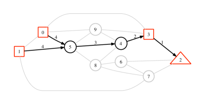
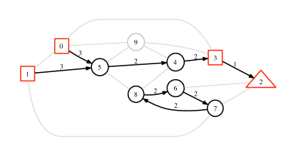
Figure 1: Left: A feasible solution of the RSTP for a small graph of ten nodes in the normal representation. Right: A feasible configuration for the flat representation.

Finally, the computation for the corresponding (13) for the flat model can be also carried out in overall time proportional to $D\left|E\right|$ per iteration. The MS equation is

$$h_{ij}^{t+1}\left(d_{ij}\right) = \max_{\begin{subarray}{c}\mathbf{d}_{i\setminus j}:\\ \psi^{\prime}_{i}\left(\mathbf{d}_{i}\right)=1\end{subarray}}\big{\{}-c_{i}\mathbb{I}\left[\mathbf{d}_{i}\equiv\mathbf{0}\right]-\sum_{k\in V\left(i\right)}w_{ik}\mathbb{I}\left[d_{ik}>0\right]+\sum_{k\in V\left(i\right)\setminus j}h_{ki}^{t}\left(d_{ki}\right)\big{\}}$$ (25)

$$= \max\left\{M_{ij}\left(d_{ij}\right),M_{ij}^{flat}\left(d_{ij}\right)\right\}$$ (26)

where

$$M_{ij}\left(d_{ij}\right) = \max_{\begin{subarray}{c}\mathbf{d}_{i\setminus j}:\\ \psi_{i}\left(\mathbf{d}_{i}\right)=1\end{subarray}}\left\{-c_{i}\mathbb{I}\left[\mathbf{d}_{i}\equiv\mathbf{0}\right]-\sum_{k\in V\left(i\right)}w_{ik}\mathbb{I}\left[d_{ik}>0\right]+\sum_{k\in V\left(i\right)\setminus j}h_{ki}^{t}\left(d_{ki}\right)\right\}$$ (27)

$$M_{ij}^{flat}\left(d_{ij}\right) = -w_{ij}\mathbb{I}\left[d_{ij}>0\right]+\max_{\begin{subarray}{c}\mathbf{d}_{i\setminus j}:\\ \psi_{i}^{flat}\left(\mathbf{d}_{i}\right)=1\end{subarray}}\sum_{k\in V\left(i\right)\setminus j}\left\{h_{ki}^{t}\left(d_{ki}\right)-w_{ik}\mathbb{I}\left[d_{ik}>0\right]\right\}$$ (28)

The term $M$ corresponds to the MS equation for the normal model that can be computed as described in Subsection III.4. For $i$ such that $c_{i}=0$, the term $M^{flat}$ will be computed as follows. For $d_{ij}\neq 0$

$$\begin{cases}M_{ij}^{flat}\left(d_{ij}\right)=-w_{ij}+\max_{k\in V\left(i\right)\setminus j}\left\{h_{ki}^{t}\left(d_{ij}\right)+\sum_{l\in V\left(i\right)\backslash j,k}h_{li}^{t}(0)\right\}&\quad\mbox{ for }d_{ij}>0\\ M_{ij}^{flat}\left(d_{ij}\right)=\max_{k\in V\left(i\right)\setminus j}\left\{h_{ki}^{t}\left(d_{ij}\right)-w_{ik}+\sum_{l\in V\left(i\right)\backslash j,k}h_{li}^{t}(0)\right\}&\quad\mbox{ for }d_{ij}<0\end{cases}$$ (29)

The restricted maxima in (29) for all neighbors $j\in V\left(i\right)$ can be computed in time proportional to $\left|V\left(i\right)\right|$ as in (20). For $d_{ij}=0$ instead,

$$M_{ij}^{flat}\left(0\right)=\max_{d>0}\max_{\begin{subarray}{c}k,\,l\in V\left(i\right)\setminus j\\ k\neq l\end{subarray}}\bigg{\{}h_{ki}^{t}\left(d\right)+h_{li}^{t}\left(-d\right)-w_{il}+\sum_{m\in V\left(i\right)\backslash j,k,l}h_{mi}^{t}(0)\bigg{\}}$$ (30)

For each $d>0$, the internal $\max$ can be computed for all $j\in V\left(i\right)$ again in time proportional $\left|V\left(i\right)\right|$, in a way similar to the one described in (20) but this time recording the first three maximums of the quantities in braces instead of first two. In summary, also using the flat rule the number of needed elementary operations per iteration is $\Theta\left(D\left|E\right|\right)$.

IV A Belief Propagation-Inspired Heuristics

IV.1 Pruned Trees

One drawback of the MS heuristics with respect to local search based ones consists in the fact that until convergence of the algorithm, decisional variables are in a state of inconsistency, incompatible with a single feasible solution of the problem. A way of obtaining feasible trees after a few iterations, but long before convergence, is to use simple heuristics for the SPG and for the PCSPG that use information carried by MS fields instead of the original edge and node weights. This procedure will be carefully designed so that in case of convergence of the MS equations the outcome of the heuristics is identical to the solution given by the decisional variables of the MS solution. These strategies become helpful and decisive when we deal with limited available time, especially for very large instances, and of course in cases in which plain MS equations do not converge.

To give an example we plot in Fig. (2) the outcomes of the heuristics (labelled as “N”, “J” and “W” which are described in Subsection IV.2) and MS, before convergence of the algorithm, for one of the instances of 11th DIMACS Implementation Challenge, the cc3-12nu instance. Points represent feasible solutions to the PCSPG at any time while we trace the minimum of the energy provided by each variant using a dashed line. At time zero we plot the energy of the trivial solution in which the tree only contains its root. We see that after few hundreds of seconds the heuristics can give a more energetically favored solution which improves in time until it coincides with the MS energy at convergence.

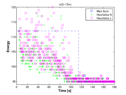
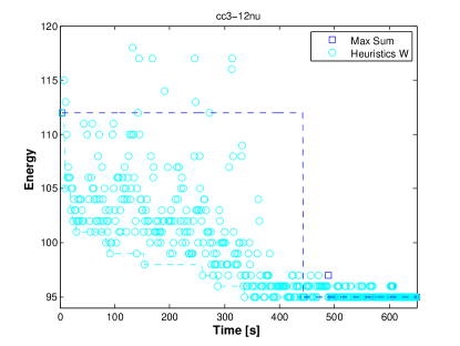
Figure 2: Energy of the solution to the PCSPG as function of time on instance cc3-12nu

IV.1.1 Minimum Spanning Tree and Shortest Path Tree

At each iteration $t$ we compute a set of modified weights $w_{ij}^{t}$ of the graph $G=(V,\,E)$ which are functions of the local fields $H_{ij}^{t}$ or cavity fields $h_{ij}^{t}$. We build a feasible Steiner tree on this re-weighted graph as follows. First, we compute a spanning tree $T_{H}(V_{H},E_{H})$ (using either (a) Minimum Spanning Tree (MST) or (b) the Shortest Path Tree (SPT) by Prim or Dijkstra’s algorithm respectively). Afterwards, we apply the following pruning procedure: starting from each leaf node $i\in V_{H}$ with $V(i)=\{j\}$, we check whether $w_{ij}>c_{i}$. In this case adding node $i$ to the solution is energetically unfavorable and we delete $i$ and $(i,j)$ from $T_{H}$. We recursively repeat this procedure until no such leaf is found. Weights $w_{ij}^{t}$ will be computed in two alternative ways:

1. Reweighting edges. A first way uses only information contained in cavity fields $H_{ij}^{t}$: we set $w_{ij}^{t}=\max_{d\neq 0}H_{ij}^{t}\left(d\right)$. This quantity will be strictly positive if the decisional variable $d_{ij}^{\star}=0$ and will be zero if $d_{ij}^{\star}\neq 0$.

2. Reweighting nodes. A second way of assigning auxiliary costs to edges takes into account the prediction of MS regarding the presence of each vertex $i$ in the solution. From the equations, a decisional variable can be assigned to the presence of node $i$ at depth $d\geq 0$ by setting

   $$h_{i}\left(d\right) = \max_{k\in V(i)}\left\{h_{ik}^{t}(-d)+\sum_{l\in V(i)\setminus k}\max\left\{h_{li}^{t}\left(d+1\right),h_{li}^{t}\left(0\right)\right\}\right\}\quad\mbox{ for }d>0$$

   $$h_{i}\left(0\right) = \sum_{k\in V(i)}h_{ki}^{t}(0)-c_{i}$$ (31)

   We will thus force the presence of nodes $i$ such that $\max_{d>0}h_{i}\left(d\right)>h_{i}\left(0\right)$, by adding a large prize $C$ to edges connecting nodes not satisfying this property.

IV.1.2 Goemans-Williamson heuristics

For the PCSPG, in addition to the MST and the SPT, we implement the Goemans-Williamson (GW) algorithm. For the theoretical reasoning and a detailed description see Goemans:1992:GAT:139404.139468 and Goemans:1996:PMA:241938.241942 . Here we briefly explain the main steps of the algorithm and how we modify the weights and the prizes of the graph in order to include the (partial) MS result within the heuristics.

The algorithm consists in two steps, the “growth” stage and the “pruning” stage. In the first one we partition vertices in clusters that are merged and ignored during the iterations until one significant cluster remains; the more a cluster contains profitable and low cost connected nodes, the more the cluster will have the chance of being the final one. The second stage finds a solution of minimum energy for the PCSPG within the nodes of the final cluster.

Before applying the algorithm we modify prizes and weights in the following way. For each node we compute $h_{i}=\max_{d}h_{i}(d)\,-h_{i}(0)$ defined in (31). If $h_{i}$ is positive, node $i$ is present in the intermediate solution and so we increase the prize $c_{i}$ of a large constant $C$; otherwise it keeps its original prize. In this way we favor those clusters containing nodes with zero original prize but predicted by MS as Steiner nodes. Moreover, we modify edges connecting nodes $i:\,h_{i}<0$ by adding $C$ to the original weight so that clusters whose members are not included in MS solution are penalized.

IV.2 Labeling

Several approaches and techniques have been proposed in Subsection IV.1, most of them were not present in the original algorithm that competed in DIMACS challenge. Experiments are labelled depending on which model, heuristics and assignment of weights and/or prizes have been used. All the features of the final algorithm correspond to the following labels:

• “O”: this is the original version of the algorithm which competed in the challenge and appear in the official results as “polito”. It consists in the Max-Sum algorithm for the normal model joined to the MST; weights are modified as described in Reweighting edges 1.

• “N”: we implement the MST heuristics in which weights are computed according to Reweighting nodes 2.

• “J”: here we use the SPT heuristics and weights are modified as in Reweighting edges 1.

• “W”: the heuristics is the GW reported in Subsection IV.1.2.

• “F”: we use the flat model described in Subsection III.5. If no additional labels are included, we refer to the MST heuristics with modified weights as in Reweighting edges 1.

Labels can be also combined, e.g. “F J” corresponds to the Flat model with Shortest Path Tree heuristics.

IV.3 Rooting

The PCSPG and SPG variants of the problem are undirected and unrooted but the formalism introduced in Section II needs to select a root node among the profitable or terminal nodes, for the PCSPG and SPG variants respectively. It is always possible to choose a random terminal for the SPG but there is no clear strategy for the PCSPG. Moreover, the choice of a random terminal for the SPG using the normal model could lead to a suboptimal solution for a limited depth $D$. Here we propose one rooting procedure for each variant.

IV.3.1 SPG rooting

Since the running time per iteration is $\Theta\left(D|E|\right)$, it is convenient to select as root the terminal that allows a representation with a small parameter $D$. A straightforward heuristics consists then in finding the terminal for which the maximum hop distance to other terminals is the smallest. This can be computed simply by an application of Breadth-First Search for each root candidate, in time proportional to $\left|K\right|\left|E\right|$ where $\left|K\right|$ is the number of terminals.

IV.3.2 PCSPG rooting

The procedure reported in this section is the same used in biazzo_performance_2012 . Add an extra root node $r$ and connect it to all profitable vertices with extra edges of identical very large weight $\mu$. The optimal PCSPG solution in this modified graph consists trivially in a single node tree $\left\{r\right\}$, since the addition of anything else carries a cost $\mu$ that makes it unprofitable. Nevertheless, the MS algorithm provides additional information besides the non-informative optimal result. Consider the “second” optimum solution of the problem. The root node $r$ will be connected to one (and only one) vertex of the original graph, since adding additional edge costs equal to $\mu$ will be cost-wise inconvenient. This vertex can be identified by computing $j^{*}\in\arg\max_{j}H_{jr}\left(1\right)$. Now clearly, nontrivial (unrooted) solutions of the original problem are in one to one correspondence with $r$-rooted solutions of the modified problem with only one neighbor of $r$ (and the difference in cost is simply $\mu$). Unfortunately, the information contained in MS fields is insufficient to reconstruct the full “second” optimal tree of the modified graph so a second run of the MS algorithm in the original graph, using $j^{*}$ as root is needed.

IV.4 Reinforcement

As explained in biazzo_performance_2012 ; bailly-bechet_prize-collecting_2009 ; bailly-bechet_finding_2011 , the reinforcement procedure speeds up and aids convergence of the MS algorithm but adds an additional parameter $\gamma_{1}$. Smaller values of $\gamma_{1}$ lead typically to better solutions at the cost of longer convergence times. We adopted the following approach: we start the MS algorithm with a large value of $\gamma_{1}\sim 10^{-2}$. Then we iteratively halve $\gamma_{1}$ and run again MS until $\gamma_{1}\sim 10^{-5}$. We can stop the loop in $\gamma_{1}$ if the energy gap between the new solution and the old one is significantly small since reducing again the parameter typically does generally not bring a significant improvement.

IV.5 Depth

The depth parameter $D$ is fundamental in the algorithm described in this work. It unequivocally delimits the space of the solutions since MS will provide $D$-bounded trees; furthermore the computational time depends linearly on $D$. Choosing a small depth reduces the running time but this can affect the quality of the solution: for the SPG if $D$ is not sufficiently large the connection of all terminals is impossible and in the PCSPG some profitable nodes cannot be reached. Larger values of $D$ implies a larger solution space where the optimum may be better. Thus we need to guarantee that all profitable vertices, or terminals, can be connected within the tree and then let the algorithm choose the optimal subgraph.

The computation of the minimum value of the depth $D_{min}$ uses again a Breadth-First Search procedure. We start searching from the predefined root and we save the distances, in hops, of the shortest paths between the root and any profitable vertex. We then choose as starting value of $D$, the maximum value among all these lengths. Notice that for the flat representation $D_{min}$ can be taken equal to the number of profitable vertices.

IV.6 Running schemes

In the following we explain two operative procedures that will be used for different experiments regarding the SPG and the PCSPG variants.

• D-increasing scheme. Once we have determined the proper value of $D_{min}$ as in Subsection IV.5 we apply MS and the heuristics following the reinforcement scheme described in Subsection IV.4. The process is repeated for increasing values of $D$ until the predefined running time is over.

• D-bounded scheme. Here we run the algorithm using a unique value of $D$. Simulations stop either because the reinforcement scheme in Subsection IV.4 or the available time is over.

V Results for Scale-free and Grid-like graphs

In this Section we report the performances of our new developments for two classes of graphs which model very well real-world networks, namely, the scale-free and the grid graphs. We will show here that the introduction of heuristics in Section IV guarantees feasible solutions after few iterations of MS even for loopy graphs and we will underline the improvements carried by the flat model for particular instances. We show the results of “N”, “J” and “W” (combined to the normal or to the $flat$ model) and we compare them to the results obtained by the “old” heuristic, “O”; quantitatively we compute the percentage gap between the energy given by algorithm $x$ and algorithm $y$ as:

$$Gap(x,\,y)=\frac{x-y}{y}\cdot 100$$ (32)

where $x$ represents one of our “new” enhancements and $y$ the “O” algorithm; the more the gap is negative the more $x$ outperforms $y$.

Experiments were run on a Multi-Core AMD opteron 2600Mhz server, where most of the cases we use the D-increasing scheme in Subsection • ‣ IV.6 for a running time of 600 s; if different schemes are used they will be precised in each section.

Most relevant results for single-instance problems are reported in several tables in Appendix A and B that have all the same structure. The first column contains the name of the instances, the second one displays the best energy found by the best algorithm that is reported in the third section. The remaining columns list the running time needed by the best algorithm, the “O” result and the gap computed as in (32) between the best energy and the “O” energy of the “old” algorithm. In some specific frameworks we also propose averaged results over different realizations of the same graph to confirm evidences suggested by single-instance energies.

Instances names give clear information about graph properties. The first letters identify the type of graph, i.e. can be either “SF” or “G” depending on we are dealing with a scale-free network or a grid graph. They also contain the number of nodes and the number of terminals that are followed by letters $n$ and $a$ respectively, while a suffix “-p” is added for the PCSPG instances. Grid-graph names also reveal the nodes layout on the graph. For instance, the graph G_100x100x2_a10 is a 3d grid graph of size 100x100x2 that contains 20000 nodes, 10 of which are terminals and we aim to solve a SPG.

V.1 Performances of Max Sum against heuristics

To give an example of the efficiency of the MS-guided heuristics we create 5 grid graphs of size 10x10x10 containing terminals in the range [10, 410] and 5 scale-free networks of $10^{3}$ nodes and 100 terminals with edges in the interval [2991, 10879] on which we solve the SPG. In Table 1 and 2 we report the energies achieved by “O” algorithm, MS and the MST without the reweighting scheme introduced by “O”. Energies of the MST algorithm are averaged over 10 realizations of each graph, instead, for both “O” and MS we run the algorithms 10 times for each of the 10 instances with different initial conditions and we collect the best energies among the 10 initialitations. Then these energies will be averaged over the 10 instances. The fraction of successes over the 10$\times$10 attempts is reported in the left column of “MS conv”. In the right column we count how many times MS converged at least one time over the 10 initializations, and we normalize the number of successes with respect to the number of instances per graph.

Terminals	“O”	MS	MS	conv.	MST
10	10.56	10.80	11/100	4/10	21.82
110	56.24	61.55	6/100	2/10	77.04
210	81.76	83.13	17/100	4/10	100.93
310	103.62	103.49	25/100	6/10	120.87
410	123.44	124.10	26/100	7/10	137.23

Table 1: Average energies for “O”, MS, MST and MS convergences for grid graphs 10x10x10 as a function of the number of terminals.

Edges	“O”	MS	MS	conv.	MST
2991	34.09	33.89	30/100	4/10	40.72
4975	21.25	21.22	56/100	8/10	25.13
6951	16.53	16.92	59/100	7/10	18.52
8919	13.06	13.22	14/100	3/10	14.92
10879	10.85	10.76	30/100	3/10	12.49

Table 2: Average energies for “O”, MS, MST and MS convergences for scale-free graphs of 1000 nodes and 100 terminals as a function of the number of edges.

Results suggest that MS very seldom converge on both families of networks with an average fraction of success of 17/100 for grids and 38/100 for scale-free graphs. The heuristic “O” always outputs a solution but sometimes is suboptimal in terms of energy as we can notice from the comparison with the MS ones. Nevertheless these energies are far below of the ones of the MST heuristic with original edge weights.

V.2 Scale-free networks

The first class of networks on which we run our algorithms is the one of the scale-free graphs. Instances are generated by the Barabási-Albert model also known as preferential attachment scheme. Starting from a $N_{0}$ nodes, new nodes are added, one at the time, to the graph. Each new node is attached to $m$ different vertices with a probability that is proportional to the connectivity of the existing nodes.

In our experiments the number of nodes of the graphs is $N=10^{4}$ for SPG instances, while the initial set of nodes $N_{0}$ has cardinality $m$; all graphs have weights distributed according to the uniform distribution in the interval [0, 1].

V.2.1 SPG results

To underline the efficiency of the flat model we perform experiments on sparse scale-free networks of $10^{4}$ nodes and $m=3$. We show in Fig. (3) the energies and the gaps with respect to “O” of all the other algorithms as a function of the number of terminals for three values of the depth $D=\{3,5,7\}$ and unlimited running time. For very small values of the depth (3 and 5) the “N” variant achieves gaps of the order of $10\%$ which is significantly larger than the ones obtained by all flat-model based heuristics (“F”, “NF” and “JF”) that on average are equal to $-15\%,\,-10\%$ and $-6$% for increasing values of $D$. Only for $D=7$ the “N” variant reaches the “O” performances while the “J” heuristic gives negative gaps only for $D=3$.

In addition we show the performances for very dense graphs where the parameter $m$ changes in the interval [10, 500] and we set $a=1000$. As reported in Table 3 the “NF” variant achieves, for single-instance runs, the best performance as long as the number of edges is not very large. As $m$ increases the “N” variant outperforms all the other variants reaching gaps with respect to “O” that seem to increase, in absolute value, as we increment the number of edges.

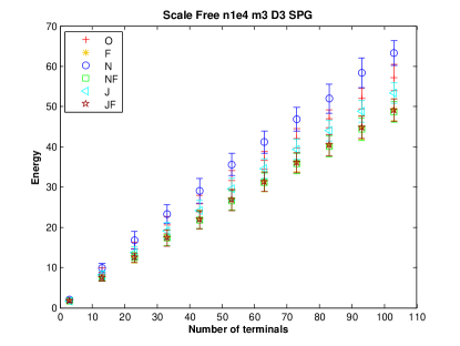
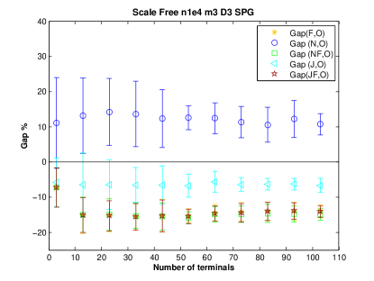
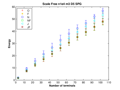
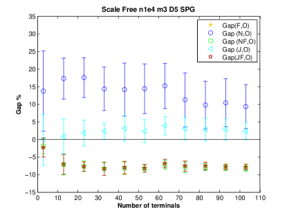
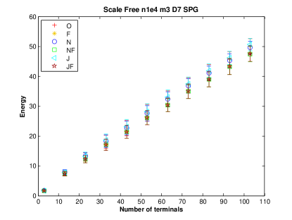
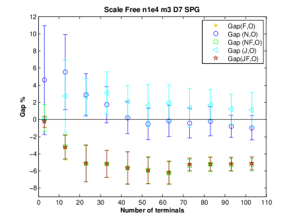
Figure 3: Left: Energy of the solution for the SPG for scale-free graph as a function of the number of terminals. Right: Energy gaps of the “F”, “N”, “NF”, “J” and “JF” heuristics with respect to “O”. From up to the bottom the depth $D$ increases.

V.3 Grid graphs

V.3.1 2d lattices

For these simulations we create 20 graph of $10^{4}$ nodes lying in a 100x100 square lattice and connected by edges whose weights distribution is uniform in the interval [0 1]. The number of terminals $a$ varies from 10 to 1000 and their prizes, for PCSPG variant only, are picked uniformly from the interval [0 15] to ensure a non-trivial optimal solution different from a single-node tree, the root, (in the case of very low prizes) and a spanning tree (in the opposite case of very large prizes).

Regarding the SPG, best solutions for single-runs are obtained through the “F” variant despite the gap with respect to the “O” algorithm is on average equals to -0.2 %. Besides, for graph containing a large number of terminals, the most performing algorithm is the “NF”. As shown in Table 4 for the PCSPG the “F” and “O” variants achieve very close results except for graph G_100x100_a10-p where the “W” heuristic reaches a gap of -5 %.

V.3.2 3d grid-graphs

Instances are 100x100x2 grid-graphs whose links have weights distributed uniformly in [0, 1] and whose terminals, for PCSPG only, have prizes in the range [0 3]. We investigate different regimes depending on how many terminals are placed on the graph.

Regarding the SPG variant, as illustrated in Table 5, the “F” variant more often gives the best solution in the case of graphs with few terminals probably because here the “depth” for the “F” algorithm is the number of terminals which is much smaller than the parameter $D_{min}$ computed as in Section IV.5.

This statement is confirmed by the statistical measure of the energies and the gaps as a function of the number of terminals that is shown in Fig. (4). The “F” variant, a part for a small positive gap in the range [20, 40], attains negative gaps that reach -10% for instances with few terminals and a constant -1% for all the range $a\in[80,140]$.

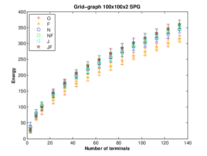
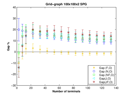
Figure 4: Left: Energy of the solution for the SPG for a grid-graph 100x100x2 as a function of the number of terminals. Right: Energy gaps of the “F”, “N”, “NF”, “J” and “JF” heuristics with respect to “O”.

For the PCSPG we investigate how energies changes when the number of terminals is in the range $[3000,10000]$. Single-instance results suggest that the “O” variant outperforms all the other up to $a\sim 4000$ where we observe that “N” and “NF” algorithms achieve best results with a gap that decreases for increasing $a$ as reported in Table 6.

To fairly compare the results of the heuristics “O”, “N”, “J” and “W” in this regime, we perform several simulations for each graph as $a$ varies in [3000, 10000] and we compare the averaged outcomes in Fig. (5). While the “J” variant attains energies as similar to the “O” ones as $a$ grows, the “N” and “W” heuristics increase their respective gaps as $a$ increases.

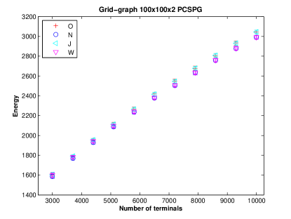
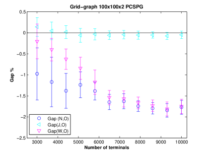
Figure 5: Left: Energy of the solution for the PCSPG for a grid-graph 100x100x2 as a function of the number of terminals. Right: Energy gaps of the “N”, “J” and “W” heuristics with respect to “O”.

VI Results of the DIMACS challenge and StenLib instances

Here we show the results of the MS algorithm combined to greedy heuristics for the SPG and PCSPG benchmark chosen for DIMACS Challenge. These instances have been selected to be particularly challenging (often the optimal solutions are not known) and to be representative of the whole set available here: http://dimacs11.cs.princeton.edu/competition.html. Additionally we report our results for a set of hard instances, called PUC, where most of the optimal solutions are still not known.

For both SPG and PCSPG variants we will need to compare outcomes provided by different algorithms or to measure the improvements of the new algorithm. According to the rules of the official competition, we use as comparison metrics the Primal Bound (PB) that is the best solution found in a fixed running time and the gap, computed as in (32), between algorithms $x$ and $y$ that will be specified in the following sections. Absolute values of the PB and the respectively gaps are collected in tables which are all displayed in Appendix C. Notice that official results are often rounded to the first decimal place and this may slightly affect the accuracy of the gaps.

As for the scale-free and grid graph, simulations were run on a Multi-Core AMD opteron 2600Mhz server, which is slightly slower than the cluster on which the challenge simulations were performed. Nevertheless, we compared the results obtained in the challenge by our submitted code on our local server with the same time limit, and the gaps of the primal bounds between “O” and “polito” are on average $\pm 0.3$% for all instances, well inside the confidence interval for these simulations. Thus we are sufficiently confident that new results can be also compared fairly with those of the challenge.

VI.1 SPG results

VI.1.1 Preprocessing

Regarding the SPG problem, a common approach is to apply some reduction or preprocessing techniques to instances. Preprocessing may significantly modify the original graph but in a way that an optimal solution of the reduced graph can be easily mapped into the minimum Steiner Tree of the original problem. The advantages of preprocessing consist in a speed up of the convergence and, often, a clear improvement of the solutions. In this work we use the preprocessing feature of the nice package Bossa, http://www.cs.princeton.edu/~rwerneck/bossa/.

We use the label “pre” for the results in which instances are preprocessed before the application of the algorithm. In all cases in which it was measured, the running time include the preprocessing time.

VI.1.2 Results for the D-increasing scheme

In the following we present the best Primal Bounds among all variants of the algorithm labelled according to Section IV.2. Experiments are performed as in the D-increasing scheme in Section• ‣ IV.6 where the running time is set to be of 7200 s.

Results are displayed in Table 7. The second column reveals the best Primal Bound found using our algorithms while the third one displays which model and/or heuristics reach such results. In the third section we report the running time of our fastest performer which is specified in brackets. The last two sections are devoted to the comparison between the best new performance and the “polito” PB.

Generally we improved our old “polito” results with some significant gaps of -5.87 % and -4.11 % for word666 and es10000fst01 instances respectively. Furthermore we notice that, globally, all “N-like” options outperforms the other variants.

In Table 8 we compare our new results to the best results of the competition. For each instance we show our PB, the best PB found in the challenge, where in brackets we report the performer that attained such result, and the last column contains the gaps between the two energies computed according to (32). Despite we are quite far from the best known bound for some instances (for example alut2625, lin36 and lin37 whose gaps are higher than 10 %), we generally approached the performance of the best challengers of the competition. Moreover, we further improved the best known energies of some solutions, like for the i640-341 and the “cc12-like” instances; such primal bounds are reported in bold letters.

Motivated by the performances of the “N-like” algorithm and by the improvements obtained on the “cc12-like” instances, we run “Npre” on the entire set of the PUC instances to which these graphs belong. Results shown if Table 13 and 14 reveals that we achieve optimal performances since all gaps between Npre and the best known energies are smaller then 0.80 %. Moreover, we reach new best known bounds for cc10-2p, cc11-2p and hc11p instances.

VI.1.3 Results for the D-bounded scheme

To underline the differences between the branching and the flat model, we run again the algorithm using the D-bounded scheme in Section • ‣ IV.6 imposing the depth equals to the number of terminals. The running time is set to 1200 s for these experiments.

For each heuristic, “N”, “O” and “J”, we compute the time interval for which the same heuristics combined with the flat model, “NF”, “F” and “JF”, provides a better solution then the normal model; the same experiment is performed for the pre-processed instances. In Fig. (6) we report such time thresholds.

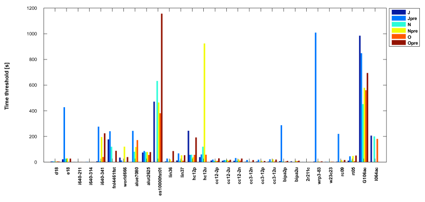
Figure 6: Time threshold Flat vs Branching model

For several instances the time threshold is equal to zero, meaning that the branching representation is always better than the flat one. A threshold of the order of hundreds of seconds appears for several instances while for es1000fst101, a rectilinear graph, and the G106ac, a “Vienna class” graph, the time interval in which the flat model (combined to almost all the heuristics) provides the best solution is significantly large.

VI.2 PCSPG results

Here we show the performance of our new enhancements “F”, “J”, “N” and “W” for the PCSPG variant. As for the SPG case we first collect our best primal bounds and we compare them to the “polito” results of the challenge. Afterwards, we show the measure of the gap with respect to the three best algorithms of the competition, “KTS”, “staynerd” and “mozartballs”. We perform simulations using the operative scheme in Section • ‣ IV.6 for a running time of 7200 s.

As plotted in Table 9 we find that the best performer is “F” that outputs the best PB for 27 instances over 32 but the more significant improvements are given by “W” for the K400-7, hands04 and handbd13 instances with a gap of -7 %, -10% and -27 % respectively; the fastest performer instead is the “N” variant.

In Table 10 we show the results of our best performers compared to “KTS”, “staynerd”, “mozartballs” and “polito” algorithms of the competition. Energies are now well comparable to the best known PB with an average gap of 0.1 % for 29 instances. Moreover, we achieve the best known energy for hc10p, hc11u, hc12u and cc12-2nu by our new algorithm; these results are reported in bold letters in Table 10. Note that additionally, for the instance hc12p, the best known energy is the one obtained by “polito”, i.e. the “O” variant.

VI.3 Non-reweighting scheme results

In order to underline the improvements of the MS-based reweighting scheme for these hard instances, we compare them to the PB provided by the heuristics (pruned Minimum Spanning Tree, pruned Shortest Path Tree and Goemans-Williamson heuristics) for the SPG and PCSPG instances with original weights on edges. As reported in Table 11 and 12 energies in columns “MST”, “SPT” and “GW” (for Prize-collecting only) are far from being comparable to the performances of the re-weighted scheme, labelled as “MS reweighting”, and thus to the state-of-the-art algorithms of the challenge.

VII Conclusion

In this work, we presented several improvements for a message-passing approach to several variants of the Steiner Tree Problem on graphs. A first improvement is the incorporation of heuristics that are able to transform partial information coming from an intermediate state of the messages before convergence into feasible solutions. This may be useful when the computation time at disposal is short, but it is of particular importance because it forces the algorithm to output solutions even in cases in which the tree-like approximation is inaccurate and reinforced Max-Sum equations do not converge. This resulted in the variant that we called “O” in this manuscript, that participated in the 2014 DIMACS Challenge with encouraging results. We give a detailed report on the outcome of the Challenge.

With respect to the results in the Challenge, we report here several further improvements, including two different heuristics, the “W”, “N” and “J” variants and their combinations. Many strategies have been explored and reported here, with the outcome that the “N” variant is the best overall, but some of the other variants give advantages for some instance types. During this development we derived an “edge variables” formulation, that allows to cope with a modified flat model that removes one impediment of past approaches of this type; namely the need of a large maximum hop-distance $D$. This results in the “F” variant of the algorithm, that give advantages in particular on structured networks including meshes and scale-free graphs. Moreover the “edge variables” formulation presented here is also in principle able to accommodate other constraints, such as degree ones, in a simple way.

Appendix A Results for Scale free Graphs

Instance	PB	Algo	Time [s]	“O” PB	Gap %
SF_n1e4_m10_a1e3	$115.92$	N	$595.97$	$116.86$	$-0.80$
SF_n1e4_m36_a1e3	$33.54$	NF	$266.24$	$36.24$	$-7.45$
SF_n1e4_m62_a1e3	$19.28$	NF	$381.05$	$20.64$	$-6.59$
SF_n1e4_m87_a1e3	$14.21$	NF	$492.69$	$15.18$	$-6.36$
SF_n1e4_m113_a1e3	$11.37$	NF	$443.22$	$12.67$	$-10.26$
SF_n1e4_m139_a1e3	$9.14$	NF	$602.81$	$10.39$	$-12.00$
SF_n1e4_m165_a1e3	$8.89$	N	$487.00$	$8.92$	$-0.41$
SF_n1e4_m191_a1e3	$7.24$	N	$29.51$	$7.33$	$-1.24$
SF_n1e4_m216_a1e3	$6.80$	N	$325.07$	$6.90$	$-1.44$
SF_n1e4_m242_a1e3	$5.84$	N	$40.44$	$5.92$	$-1.48$
SF_n1e4_m268_a1e3	$5.67$	N	$454.76$	$5.75$	$-1.40$
SF_n1e4_m294_a1e3	$5.05$	N	$60.07$	$5.14$	$-1.79$
SF_n1e4_m319_a1e3	$4.58$	N	$55.55$	$4.76$	$-3.83$
SF_n1e4_m345_a1e3	$4.07$	N	$46.22$	$4.19$	$-3.05$
SF_n1e4_m371_a1e3	$4.05$	N	$49.51$	$4.29$	$-5.63$
SF_n1e4_m397_a1e3	$3.86$	N	$76.40$	$4.05$	$-4.69$
SF_n1e4_m423_a1e3	$3.44$	N	$106.89$	$3.74$	$-7.92$
SF_n1e4_m448_a1e3	$3.29$	N	$80.44$	$3.62$	$-9.01$
SF_n1e4_m474_a1e3	$3.14$	N	$96.80$	$3.42$	$-8.00$
SF_n1e4_m500_a1e3	$3.10$	N	$104.78$	$3.35$	$-7.37$

Table 3: Best Primal Bounds for SPG on Scale Free networks, fixed a

Appendix B Results for Grid Graphs

Instance	PB	Algo	Time [s]	“O” PB	Gap %
G_100x100_a10-p	$50.36$	W	$13.977$	$53.18$	$-5.29$
G_100x100_a62-p	$215.10$	O	$25.072$	$215.10$	$-$
G_100x100_a114-p	$305.92$	O	$8.24$	$305.92$	$-$
G_100x100_a166-p	$363.03$	F	$20.32$	$369.46$	$-1.74$
G_100x100_a218-p	$421.11$	F	$206.27$	$427.23$	$-1.43$
G_100x100_a271-p	$477.41$	O	$13.62$	$477.41$	$-$
G_100x100_a323-p	$532.13$	F	$34.91$	$538.51$	$-1.18$
G_100x100_a375-p	$554.55$	O	$98.42$	$554.55$	$-$
G_100x100_a427-p	$581.97$	F	$168.98$	$586.18$	$-0.72$
G_100x100_a479-p	$624.02$	O	$16.64$	$624.02$	$-$
G_100x100_a531-p	$654.29$	O	$16.22$	$654.29$	$-$
G_100x100_a583-p	$673.97$	F	$73.10$	$675.27$	$-0.19$
G_100x100_a635-p	$725.31$	O	$12.44$	$725.31$	$-$
G_100x100_a687-p	$742.67$	O	$13.62$	$742.67$	$-$
G_100x100_a739-p	$765.91$	F	$247.15$	$770.46$	$-0.59$
G_100x100_a792-p	$788.36$	F	$261.86$	$795.58$	$-0.91$
G_100x100_a844-p	$817.39$	O	$14.45$	$817.39$	$-$
G_100x100_a896-p	$854.57$	O	$13.51$	$854.57$	$-$
G_100x100_a948-p	$872.88$	O	$11.95$	$872.88$	$-$
G_100x100_a1000-p	$890.94$	O	$10.96$	$890.94$	$-$

Table 4: Primal Bounds for the PCSPG on 2d grid graphs

Instance	PB	Algo	Time [s]	“O” PB	Gap %
G_100x100x2_a10	$78.07$	O	$51.142$	$78.07$	$-$
G_100x100x2_a62	$203.13$	O	$14.114$	$203.13$	$-$
G_100x100x2_a114	$286.96$	F	$26.15$	$290.06$	$-1.07$
G_100x100x2_a166	$358.52$	F	$25.08$	$362.57$	$-1.12$
G_100x100x2_a218	$424.50$	F	$31.80$	$429.52$	$-1.17$
G_100x100x2_a271	$468.21$	O	$27.04$	$468.21$	$-$
G_100x100x2_a323	$495.39$	F	$57.39$	$503.96$	$-1.70$
G_100x100x2_a375	$552.07$	F	$32.98$	$556.24$	$-0.75$
G_100x100x2_a427	$578.32$	F	$39.57$	$586.57$	$-1.41$
G_100x100x2_a479	$608.99$	F	$55.25$	$609.44$	$-0.07$
G_100x100x2_a531	$635.29$	F	$43.12$	$644.63$	$-1.45$
G_100x100x2_a583	$662.13$	F	$44.29$	$665.76$	$-0.55$
G_100x100x2_a635	$692.11$	F	$47.99$	$697.51$	$-0.77$
G_100x100x2_a687	$716.63$	F	$50.44$	$719.79$	$-0.44$
G_100x100x2_a739	$755.78$	O	$30.24$	$755.78$	$-$
G_100x100x2_a792	$780.45$	F	$56.66$	$781.62$	$-0.15$
G_100x100x2_a844	$797.13$	F	$38.55$	$804.08$	$-0.86$
G_100x100x2_a896	$822.84$	F	$42.10$	$823.93$	$-0.13$
G_100x100x2_a948	$843.94$	F	$49.80$	$847.32$	$-0.40$

Table 5: Primal Bounds for the SPG on 3d grid graphs with few terminals

Instance	PB	Algo	Time [s]	“O” PB	Gap %
G_100x100x2_a1000-p	$875.85$	O	$45.04$	$875.85$	$-$
G_100x100x2_a1474-p	$1057.83$	O	$46.75$	$1057.83$	$-$
G_100x100x2_a1947-p	$1234.77$	O	$43.86$	$1234.77$	$-$
G_100x100x2_a2421-p	$1395.98$	O	$46.19$	$1395.98$	$-$
G_100x100x2_a2895-p	$1554.88$	O	$47.62$	$1554.88$	$-$
G_100x100x2_a3368-p	$1697.28$	O	$46.85$	$1697.28$	$-$
G_100x100x2_a3842-p	$1824.59$	N	$34.68$	$1833.18$	$-0.47$
G_100x100x2_a4316-p	$1941.98$	N	$53.69$	$1955.73$	$-0.70$
G_100x100x2_a4789-p	$2036.87$	NF	$241.08$	$2056.08$	$-0.93$
G_100x100x2_a5263-p	$2122.72$	NF	$230.64$	$2152.41$	$-1.38$
G_100x100x2_a5737-p	$2229.83$	NF	$169.36$	$2264.99$	$-1.55$
G_100x100x2_a6211-p	$2339.31$	N	$40.47$	$2382.05$	$-1.79$
G_100x100x2_a6684-p	$2414.71$	N	$516.42$	$2457.86$	$-1.76$
G_100x100x2_a7158-p	$2524.14$	N	$52.56$	$2575.23$	$-1.98$
G_100x100x2_a7632-p	$2609.18$	NF	$243.35$	$2658.92$	$-1.87$
G_100x100x2_a8105-p	$2700.71$	NF	$456.12$	$2758.35$	$-2.09$
G_100x100x2_a8579-p	$2775.56$	N	$34.92$	$2834.97$	$-2.10$
G_100x100x2_a9053-p	$2863.76$	NF	$362.59$	$2919.05$	$-1.89$
G_100x100x2_a9526-p	$2953.47$	N	$211.22$	$3019.45$	$-2.19$
G_100x100x2_a10000-p	$3012.83$	N	$42.95$	$3074.09$	$-1.99$

Table 6: Primal Bounds for the PCSPG on 3d grid graphs with many terminals

Appendix C Dimacs and Stenlib results

Instance	New PB	Algo	Time [s]	“polito” PB	Gap %
d18	223	All	2.97 (Fpre)	224	$-0.45$
e18	564	All	112.78 (NFpre)	565	$-0.18$
i640-211	11984	All	851.79 (Opre)	11984	$0.00$
i640-314	35532	N NF	223.53 (N)	35532	$0.00$
i640-341	32042	NFpre	2164.31	32047	$-0.02$
fnl4461fst	189367	Npre	3759.34	192847	$-1.80$
world666	122971	N	94.37	130516	$-5.78$
alue7080	66624	NF	100.96	67847	$-1.80$
alut2625	40183	Npre	1042.46	41501	$-3.18$
es10000fst01	733237957	Npre	1232.63	764631264	$-4.11$
lin36	64486	Npre	399.04	64052	$0.68$
lin37	112886	Npre	892.89	114001	$-0.98$
hc12p	236075	N Npre	3664.50 (N)	236042	$0.01$
hc12u	2269	Opre J Jpre N Npre	4883.88 (Npre)	2265	$0.18$
cc12-2p	121056	N	7077.52	121091	$-0.03$
cc12-2u	1174	N Npre	6330.21 (Npre)	1177	$-0.25$
cc12-2n	613	Npre	4425.05	615	$-0.33$
cc3-12n	111	All	20.60 (Opre)	111	$0.00$
cc3-12p	19003	N Npre	5750.94 (N)	18932	$0.38$
cc3-12u	185	All	2331.35 (N)	186	$-0.54$
bipa2p	35285	Npre	1927.36	35336	$-0.14$
bipa2u	338	All	118.86 (NF)	339	$-0.29$
2r211c	89000	Opre J Jpre N Npre	615.75 (Jpre)	90000	$-1.11$
wrp3-83	8301057	N	1191.62	8301263	$0.00$
w23c23	691	F Fpre JF JFpre NF NFpre	3541.60 (NF)	693	$-0.29$
rc09	120450	Npre	4176.39	122358	$-1.56$
rt05	58286	F	27.08 (F)	59147	$-1.46$
G106ac	40396063	N	7088.62	40346932	$0.12$
I064ac	188849475	J	4678.88	188479558	$0.20$
s5	25210	All	124.29 (NF)	25210	$0.00$

Table 7: Best PB for all the SPG instances and comparison with “polito” results

Instance	PB	Best PB of the Challenge	Gap %
d18	223	223 (AB mozartballs scipjack staynerd)	$0.00$
e18	564	564 (mozartballs scipjack staynerd)	$0.00$
i640-211	11984	11984 (polito scipjack)	$0.00$
i640-314	35532	35532 (polito staynerd)	$0.00$
i640-341	32042	32047 (polito)	$-0.02$
fnl4461fst	189367	182527 (PUW)	$3.75$
world666	122971	122467 (mozartballs PUW scipjack staynerd)	$0.41$
alue7080	66624	62514 (PUW)	$6.57$
alut2625	40183	35471 (PUW)	$13.28$
es10000fst01	733237957	716559567 (mozartballs)	$2.33$
lin36	64486	55608 (PUW)	$15.97$
lin37	112886	99560 (PUW)	$13.38$
hc12p	236075	236042 (polito)	$0.01$
hc12u	2269	2262 (staynerd)	$0.31$
cc12-2p	121056	121091 (polito)	$-0.03$
cc12-2u	1174	1177 (polito)	$-0.25$
cc12-2n	613	615 (polito)	$-0.33$
cc3-12n	111	111 (mozartballs polito PUW scipjack staynerd)	$0.00$
cc3-12p	19003	18865 (mozartballs)	$0.73$
cc3-12u	185	185 (mozartballs PUW staynerd)	$0.00$
bipa2p	35285	35336 (polito)	$-0.14$
bipa2u	338	337 (mozartballs staynerd)	$0.30$
2r211c	89000	89000 (mozartballs PUW scipjack staynerd)	$0.00$
wrp3-83	8301057	8300906 (PUW)	$0.00$
w23c23	691	689 (mozartballs staynerd)	$0.29$
rc09	120450	111005 (mozartballs staynerd)	$8.51$
rt05	58286	51354 (PUW)	$13.50$
G106ac	40396063	36920936 (mozartballs staynerd)	$9.41$
I064ac	188849475	186852309 (PUW)	$1.07$
s5	25210	25210 (mozartballs polito PUW scipjack staynerd)	$0.00$

Table 8: Best PB for all the SPG instances and comparison with the best results of the Challenge

Instance	PB	Algo	Time [s]	“polito” PB	Gap %
C13-A	236	F J N W	1.23 (N)	237	$-0.42$
C19-B	146	F J N W	2.62 (N)	146	$0.00$
D03-B	1509	F J N W	5.79 (N)	1510	$-0.07$
D20-A	536	F J N W	4.64 (N)	536	$0.00$
P400-3	2951725	F J N W	1.64 (N)	2951725	$0.00$
P400-4	2852956	F J N W	4.30 (N)	2852956	$0.00$
K400-7	485587	W	2289.60	523885	$-7.31$
K400-10	401032	W	1086.08	406365	$-1.31$
hc10p	59682	W	7140.50	59813	$-0.22$
hc11u	1115	F J N	1988.85 (N)	1120	$-0.45$
hc12p	235132	F J N	5463.03 (N)	235043	$0.04$
hc12u	2216	F J N	6071.29 (N)	2227	$-0.49$
bip52nu	222	F	3093.53	223	$-0.45$
bip62nu	214	F J N W	4.32 (N)	214	$0.00$
cc3-12nu	95	F J N W	26.43 (N)	95	$0.00$
cc12-2nu	565	F N	2789.17 (F)	567	$-0.35$
i640-001	2932	F J N W	0.42 (N)	3053	$-3.96$
i640-221	8430	F	5466.72	8626	$-2.27$
i640-321	28790	F	6949.88	28821	$-0.11$
i640-341	29679	F	2037.28	29713	$-0.11$
a2000RandGraph-2	1483.84	F J N W	10.04 (N)	1484.2	$-0.02$
a4000RandGraph-3	3406.62	F J N W	6.74 (N)	3407.5	$-0.03$
a8000RandGraph-1-2	4719.97	F J N	5552.40 (N)	4722.8	$-0.06$
a14000RandGraph-1-5	9475.59	F J N	690.66 (N)	9475.6	$0.00$
handsd04	525.86	W	1470.15	584.1	$-9.97$
handbd13	13.23	F J N W	100.15 (N)	18.1	$-26.91$
handsi03	56.23	F J N	31.95 (J)	56.3	$-0.12$
handbi07	151.04	F J N W	88.46 (W)	151.1	$-0.04$
drosophila001	8273.98	W	3491.73	8288.3	$-0.17$
HCMV	7376.36	F J N W	4.62 (W)	7378.2	$-0.02$
lymphoma	3341.89	F J N W	344.67 (N)	3349.1	$-0.22$
metabol-expr-mice-1	11346.93	F J N W	2120.98 (W)	11901.9	$-4.66$

Table 9: Best PB for all the PCSPG instances and comparison with “polito” results

Instance	PB	Best PB of the Challenge	Gap %
C13-A	236	236 (KTS mozartballs staynerd)	$0.00$
C19-B	146	146 (All)	$0.00$
D03-B	1509	1509 (All)	$0.00$
D20-A	536	536 (All)	$0.00$
P400-3	2951725	2951725 (All)	$0.00$
P400-4	2852956	2852956 (All)	$0.00$
K400-7	485587	474466 (KTS mozartballs staynerd)	$2.34$
K400-10	401032	394191 (KTS mozartballs staynerd)	$1.74$
hc10p	59682	59738 (polito)	$-0.09$
hc11u	1115	1116 (mozartballs staynerd)	$-0.09$
hc12p	235132	234977 (polito)	$0.07$
hc12u	2216	2221 (KTS)	$-0.23$
bip52nu	222	222 (mozartballs)	$0.00$
bip62nu	214	214 (All)	$0.00$
cc3-12nu	95	95 (KTS mozartballs staynerd)	$0.00$
cc12-2nu	565	567 (KTS polito)	$-0.35$
i640-001	2932	2932 (All)	$0.00$
i640-221	8430	8400 (KTS mozartballs)	$0.36$
i640-321	28790	28787 (KTS)	$0.01$
i640-341	29679	29666 (KTS)	$0.04$
a2000RandGraph-2	1483.84	1483.8 (mozartballs staynerd)	$0.00$
a4000RandGraph-3	3406.62	3406.6 (mozartballs staynerd)	$0.00$
a8000RandGraph-1-2	4719.97	4720.0 (mozartballs staynerd)	$0.00$
a14000RandGraph-1-5	9475.59	9475.6 (mozartballs staynerd)	$0.00$
handsd04	525.86	493.80 (staynerd)	$6.49$
handbd13	13.23	13.20 (All)	$0.23$
handsi03	56.23	56.10 (mozartballs staynerd)	$0.23$
handbi07	151.04	151 (KTS mozartballs staynerd)	$0.03$
drosophila001	8273.98	8274 (mozartballs staynerd)	$0.00$
HCMV	7376.36	7371.5 (KTS mozartballs staynerd)	$0.07$
lymphoma	3341.89	3341.9 (KTS mozartballs staynerd)	$0.00$
metabol-expr-mice-1	11346.93	11346.9 (mozartballs staynerd)	$0.00$

Table 10: Best PB for all the PCSPG instances and comparison with the best results of the Challenge

Instance	MS reweighting	MST	SPT
d18	223	335	358
e18	564	902	892
i640-211	11984	26928	15967
i640-314	35532	55479	41186
i640-341	32042	53826	43593
fnl4461fst	189367	203167	271681
world666	122971	172983	1356820
alue7080	66624	112478	188092
alut2625	40183	89813	157660
es10000fst01	733237957	760866530	990978452
lin36	64486	145363	130588
lin37	112886	223493	233031
hc12p	236075	332813	314607
hc12u	2269	2749	2878
cc12-2p	121056	237979	175225
cc12-2u	1174	1644	1624
cc12-2n	613	1130	1116
cc3-12n	111	165	155
cc3-12p	19003	44366	26078
cc3-12u	185	245	255
bipa2p	35285	56488	45663
bipa2u	338	421	420
2r211c	89000	155000	165000
wrp3-83	8301057	8301505	8402368
w23c23	691	828	918
rc09	120450	138800	226297
rt05	58286	66236	103866
G106ac	40396063	44792419	45158294
I064ac	188849475	190392002	192238839
s5	25210	25210	25210

Table 11: Heuristics vs MS guided heuristics. Comparison of the PB for the SPG instances

Instance	MS reweightng	MST	SPT	GW
C13-A	236	305	360	309
C19-B	146	215	237	204
D03-B	1509	1819	1799	1819
D20-A	536	661	638	806
P400-3	2951725	3633310	4108109	3475372
P400-4	2852956	3649056	3785708	3577568
K400-7	485587	528817	528817	528817
K400-10	401032	434488	434488	434488
hc10p	59682	77232	77232	75181
hc11u	1115	1318	1363	1264
hc12p	235132	308065	308065	308065
hc12u	2216	2581	2666	2543
bip52nu	222	284	281	278
bip62nu	214	239	242	244
cc3-12nu	95	112	112	112
cc12-2nu	565	697	697	697
i640-001	2932	3764	3764	3764
i640-221	8430	21117	12006	11630
i640-321	28790	49605	42401	41880
i640-341	29679	49707	38085	41826
a2000RandGraph-2	1483.84	1648.58	1822.47	1645.15
a4000RandGraph-3	3406.62	3616.03	4314.37	3615.58
a8000RandGraph-1-2	4719.97	4790.86	4790.86	4790.86
a14000RandGraph-1-5	9475.59	10514.12	10514.12	10514.12
handsd04	525.86	792.61	792.61	792.61
handbd13	13.23	13.24	13.24	13.24
handsi03	56.23	56.26	56.26	56.26
handbi07	151.04	151.06	151.06	151.06
drosophila001	8273.98	8296.30	8296.30	8296.30
HCMV	7376.36	7376.84	7376.84	7376.84
lymphoma	3341.89	3410.36	3410.36	3410.36
metabol-expr-mice-1	11346.93	11885.90	11885.90	11885.90

Table 12: Heuristics vs MS guided heuristics. Comparison of the PB for the PCSPG instances

Instance	Best Known	Npre	Gap %
bip42p	24657 (opt)	24657	$0.00$
bip42u	236 (opt)	236	$0.00$
bip52p	24526	24549	$0.09$
bip52u	234	234	$0.00$
bip62p	22843	22843	$0.00$
bip62u	219	219	$0.00$
bipe2p	5616 (opt)	5616	$0.00$
bipe2u	54 (opt)	54	$0.00$
cc10-2p	35297	35269	$-0.08$
cc10-2u	342	342	$0.00$
cc11-2p	63491	63405	$-0.14$
cc11-2u	612	614	$0.33$
cc3-10p	12772	12870	$0.77$
cc3-10u	125	125	$0.00$
cc3-11p	15582	15680	$0.63$
cc3-11u	153	153	$0.00$
cc3-4p	2338 (opt)	2338	$0.00$
cc3-4u	23 (opt)	23	$0.00$
cc3-5p	3661 (opt)	3665	$0.11$
cc3-5u	36 (opt)	36	$0.00$
cc5-3p	7299 (opt)	7302	$0.04$
cc5-3u	71 (opt)	71	$0.00$
cc6-2p	3271 (opt)	3271	$0.00$
cc6-2u	32 (opt)	32	$0.00$
cc6-3p	20270 (opt)	20298	$0.14$
cc6-3u	197 (opt)	198	$0.51$
cc7-3p	56799	56835	$0.06$
cc7-3u	549	553	$0.73$
cc9-2p	17199	17225	$0.15$
cc9-2u	167 (opt)	167	$0.00$

Table 13: Best known energies for PUC instances, “bip”-like and “cc”-like classes

Instance	Best Known	Npre	Gap %
hc10p	59797	59808	$0.02$
hc10u	575	575	$0.00$
hc11p	119492	119456	$-0.03$
hc11u	1145	1153	$0.70$
hc6p	4003 (opt)	4003	$0.00$
hc6u	39 (opt)	39	$0.00$
hc7p	7905 (opt)	7906	$0.01$
hc7u	77 (opt)	77	$0.00$
hc8p	15322 (opt)	15336	$0.09$
hc8u	148 (opt)	148	$0.00$
hc9p	30242	30313	$0.23$
hc9u	292	292	$0.00$

Table 14: Best known energies for PUC instances, “hc”-like class

References

- (1) Shao-shan Carol Huang and Ernest Fraenkel. Integrating Proteomic, Transcriptional, and Interactome Data Reveals Hidden Components of Signaling and Regulatory Networks. Sci. Signal., 2(81):ra40–ra40, July 2009.
- (2) Marc Bailly-Bechet, Alfredo Braunstein, and Riccardo Zecchina. A prize-collecting steiner tree approach for transduction network inference. In Pierpaolo Degano and Roberto Gorrieri, editors, Computational Methods in Systems Biology, number 5688 in Lecture Notes in Computer Science, pages 83–95. Springer Berlin Heidelberg, January 2009.
- (3) Nurcan Tuncbag, Alfredo Braunstein, Andrea Pagnani, Shao-ShanCarol Huang, Jennifer Chayes, Christian Borgs, Riccardo Zecchina, and Ernest Fraenkel. Simultaneous reconstruction of multiple signaling pathways via the prize-collecting steiner forest problem. In Benny Chor, editor, Research in Computational Molecular Biology, volume 7262 of Lecture Notes in Computer Science, pages 287–301. Springer Berlin Heidelberg, 2012. Cited by 0002.
- (4) Ivana Ljubić, René Weiskircher, Ulrich Pferschy, Gunnar W. Klau, Petra Mutzel, and Matteo Fischetti. An Algorithmic Framework for the Exact Solution of the Prize-Collecting Steiner Tree Problem. Math. Program., 105(2-3):427–449, October 2005.
- (5) Mohsen Bayati, A. Braunstein, and Riccardo Zecchina. A rigorous analysis of the cavity equations for the minimum spanning tree. Journal of Mathematical Physics, 49(12):125206, 2008. Cited by 0012.
- (6) M. Bayati, C. Borgs, A. Braunstein, J. Chayes, A. Ramezanpour, and R. Zecchina. Statistical mechanics of steiner trees. Physical Review Letters, 101(3):037208, July 2008.
- (7) Indaco Biazzo, Alfredo Braunstein, and Riccardo Zecchina. Performance of a cavity-method-based algorithm for the prize-collecting steiner tree problem on graphs. Phys. Rev. E, 86:026706, August 2012.
- (8) Marc Mézard and Andrea Montanari. Information, Physics, and Computation. Oxford University Press, January 2009.
- (9) M. Bailly-Bechet, C. Borgs, A. Braunstein, J. Chayes, A. Dagkessamanskaia, J.-M. François, and R. Zecchina. Finding undetected protein associations in cell signaling by belief propagation. Proceedings of the National Academy of Sciences, 108(2):882–887, January 2011.
- (10) Michel X. Goemans and David P. Williamson. A general approximation technique for constrained forest problems. In Proceedings of the Third Annual ACM-SIAM Symposium on Discrete Algorithms, SODA ’92, pages 307–316, Philadelphia, PA, USA, 1992. Society for Industrial and Applied Mathematics.
- (11) Michel X. Goemans and David P. Williamson. Approximation algorithms for np-hard problems. chapter The Primal-dual Method for Approximation Algorithms and Its Application to Network Design Problems, pages 144–191. PWS Publishing Co., Boston, MA, USA, 1997.