Deep Structured-Output Regression Learning for Computational Color Constancy

Abstract

The color constancy problem is addressed by structured-output regression on the values of the fully-connected layers of a convolutional neural network. The AlexNet and the VGG are considered and VGG slightly outperformed AlexNet. Best results were obtained with the first fully-connected ”fc₆” layer and with multi-output support vector regression. Experiments on the SFU Color Checker and Indoor Dataset benchmarks demonstrate that our method achieves competitive performance, outperforming the state of the art on the SFU indoor benchmark.

I Introduction

A visual system possesses color constancy if it perceives colors almost independently of the prevailing illumination for a wide range of conditions. In digital cameras, the so-called automatic white balance aims at reaching this property. Color constancy is a desirable property in many computer vision and graphics applications where the intrinsic color of the object is needed – for accurate classification, regression, segmentation, and feature extraction [24] as well as for accurate scene rendering.

Methods aiming at achieving color constancy fall into two groups. The first estimate illumination properties of the observed scene which is followed by image color correction called chromatic adaption [2, 3] [10], [12], [16, 23, 40]. The second group, operates on an illumination invariant representations without explicitly estimating the scene illumination. The invariant features are designed or learned to depend only on reflectance characteristics or spatial structure [1, 17, 33, 39].

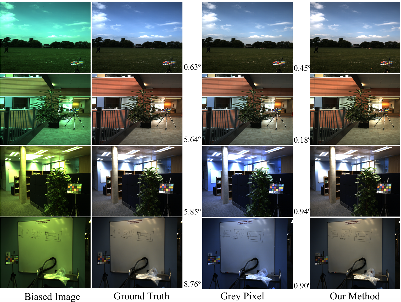
Figure 1: Image Correction of examples of the SFU Color Checker Dataset using different approaches.

We propose a novel method for estimating scene illumination color that uses a structured-output regression on the output of a single fully-connected layer from a deep net. Image color is then corrected on the basis of the estimated illumination parameters. The deep net extract visual information that has been shown to facilitate color constancy [6] as well as other computer vision task [31, 36, 38].

The structured-output regression models the cross-channel correlations, which is the main contribution of our work. In the literature [21], single-output regressor, i.e. support vector regression, has been employed to learn the relationship between observation variables and each color dimension of the target variables independently.

We show experimentally that the proposed framework achieves competitive performance comparable with several state-of-the-art methods on two popular color constancy benchmarks.

Figure 2: The proposed color constancy method consists of CNN feature extraction, multi-output regression learning and color correction.

II Related Work

Color constancy is a well-established problem. To understand the complexity of the problem, we revisit one of the simplest but yet often adopted model of image formation, i.e, the of Lambertian surfaces with purely diffuse reflection lit by constant scene illumination. In this case, the measured image color values $\rho_{i}(x,y)$ at pixel $x,y$ is a function of the global light source $I(\lambda)$, the spectral response of the sensors $S_{i}(\lambda)$, and the surface reflectance $R(x,y,\lambda)$, $\lambda$ denotes the wavelength. The dependence is captured by the following formula:

$$\rho_{i}(x,y)=\int I(\lambda)S_{i}(\lambda)R(x,y,\lambda)d\lambda,i\in\{\mbox{R,G,B}\}.$$

The formulate expresses that fact that the RGB value of each pixel is obtained by integration over wavelengths with different weights in each single channel.

In a color constancy task, $\rho$ is given, while $\rho_{gt}$ under canonical illumination is sought. We consider the case when neither camera sensibility $S(\lambda)$ nor the illumination $I$ are available, making this task under-constrained or under-determined [20].

Below, a basic introduction is given to illumination estimation algorithms. To make different assumptions unified, Van de Weijer et al. [40] proposed a formulation, which can cover different algorithms based on exploiting imagery statistics in a single image to estimate the scene illumination $I$ as the following:

$$I(n,\rho,\sigma)=K\sqrt[\rho]{\int\int{(\rho(x,y)\otimes G_{\sigma}(x,y))}^{\rho}dxdy},$$ (1)

where illumination $I$ is decided by the order $n$ of the derivative, Minkowski-norm $\rho$, and the scale parameter $\sigma$ of a Gaussian filter. Operator $\otimes$ defines convolution between the image $\rho$ and Gaussian filter $G$. $K$ is a constant added to make $I$ in unit length. By varying ($n,\rho,\sigma$) in Eq. (1), a number of existing algorithms are generated under different assumptions. For instance, GM-pixel [19], GW [10], SoG [15], gGW [40] and WP [11] are clustered as one group – zero-order statistics based methods, as they are all under the assumption that a part of images (e.g., local regions) has gray average color. In terms of higher order statistics, first-order [40] and second-order based methods [40] respectively adopt the assumption that edges or gradient of edges has gray average color intrinsically. In the light of this, illumination is measured by the offset of the average color. Gamut-mapping based methods assume that in real world, part of color spectral distribution of objects is able to be observed [2, 19]. In other words, the limited set of colors in each biased image is caused by a certain lighting condition, which encourages researchers to introduce a learning based framework to recognize canonical illumination pattern with a sufficient amount of labeled training data.

Machine learning algorithms have succeeded in learning a function directly mapping low-level image feature to illumination. Support Vector Regression (SVR) is first applied to deal with color constancy task in [21], but the performance is limited by weak predictive power of the color histogram. Bayesian approaches [22] learn the probability of illumination assuming normal-distributed reflectances. The Exemplar method [29] estimates illumination via finding nearest neighbor surfaces of a test image using an unsupervised clustering of texture and color features,

CNNs have been applied successfully to the color constancy problem. Barron et al. [5] formulate the color constancy as a 2D spatial localization task in log chromatic space using a convolutional classifier specifically designed for object localization. In Bianco et al. [6], a five-layer ad-hoc CNN is designed that combines feature generating and multi-channel regression to estimate illumination in an end-to-end way, similarly to [41]. Bianco et al. [6] compare results obtained with their five-layer ad-hoc CNN with reference – the output of layer fc₆ of an AlexNet fed into SVR. The AlexNet with SVR performed worse, but outperform most of the statistic-based methods. The selection of AlexNet and layer fc₆ is ad-hoc, no other layers or net architectures were explored.

III Methodology

The proposed deep structured-output regression color constancy method consists of three steps (see Fig. 2):

1. Calculation of the response, after the non-linearity, of the fully-connected fc₆ layer of the VGG CNN [36].

2. Illumination estimation by structured-output regression.

3. Image correction with the illumination obtained.

Below we describe the three steps in details.

III-A CNN Feature Extraction

Color constancy regression has been shown to perform well [6, 21]. CNN is a robust regressor for a number of problems [25].

The nets showing consistent performance for a number of vision problems are VGG [36, 38] and AlexNet [32]. We tested both architectures and the VGG outperformed AlexNet in all experiments (Table II). The 19-layer VGG CNN we adopted has the same structure as in [36].

We did not attempt training the VGG from scratch since the size of the available training set was limited to about 1000 samples (568 from the SFU Color Checker Dataset [22, 35] and 321 from the SFU Indoor Dataset [4]). We therefore tried only to fine-tune the VGG CNN that was pre-trained on ImageNet. However, the fine-tuned net performed worse than the original pre-trained VGG. Therefore, the original VGG CNN without fine-tuning was used in all experiments.

We experimented with features from different fully-connected layers, namely “fc₆”, “fc₇” (both having 4096 dimensions) and “fc₈” (1000 dimensions). The results are presented in Table III. CNN features from layer “fc₆” were selected as the performed the best, and can be extracted the fastest. The CNN feature is extracted from an image resized to $224\times 224$.

III-B Structured-Output Regression Learning

The regressor is trained on the set $\{(\boldsymbol{x,y})\}_{i}$, $i=1,2,\cdots,N$ includes vector-valued $\boldsymbol{y}$, where $\boldsymbol{x}$ denotes the 4096-dimensional VGG “fc₆” feature vector. The objective of structured-output [21] is to learn regression functions independently for ${y}^{l},l=1,2,3$ where $i$ denotes the color (RGB) dimensions. The single-output regression learning is formulated as:

$$\min~{}~{}~{}\dfrac{1}{2}||\boldsymbol{w}||_{2}^{2}+C\sum_{i=1}^{N}\text{loss}({y}^{l}_{i},f(\boldsymbol{x}_{i})),$$ (2)

where $\boldsymbol{w}\in\mathbb{R}^{d}$ is the weight vector to be optimized, the parameter $C$ controls the regularization trade-off and $f(\boldsymbol{x}_{i})=\phi(\boldsymbol{x}_{i})^{T}\boldsymbol{w}+b$ with $\phi(\cdot)$ is the kernel function to project $\boldsymbol{x}$ to a high-dimensional Hilbert space.

In order to take the possible correlations between output variables into account, general structured-output regression has the following formulation:

$$\min~{}~{}~{}\dfrac{1}{2}\sum_{l=1}^{3}||\boldsymbol{w}^{l}||_{2}^{2}+C\sum_{i=1}^{N}\text{loss}(\boldsymbol{y}_{i},F(\boldsymbol{x}_{i})),$$ (3)

where $F(\boldsymbol{x}_{i})=\phi(\boldsymbol{x}_{i})^{T}\boldsymbol{W}+\boldsymbol{b}$ with $\boldsymbol{W}\in\mathbb{R}^{d\times 3}$ and $\boldsymbol{b}\in\mathbb{R}^{3}$. Eq. (3) is the general formulation for multi-output regression. Adopting different loss functions leads to different regressors. Given training samples $\{(\boldsymbol{x},\boldsymbol{y})\}_{i},i=1,2,\cdots,N$, a multi-output regressor (i.e., multi-output support vector regression (MSVR) and multi-output ridge regression (MRR)) is employed to learn both the input-output relationship and latent correlations across output variables jointly.

Multi-output ridge regression (MRR) – minimizes quadratic loss function:

$$\min~{}~{}~{}\dfrac{1}{2}\sum_{l=1}^{3}||\boldsymbol{w}^{l}||_{2}^{2}+C\sum_{i=1}^{N}\|\boldsymbol{y}_{i}-(\phi(\boldsymbol{x}_{i})^{T}\boldsymbol{W}+\boldsymbol{b})\|_{2}^{2}.$$ (4)

It has a closed-form solution based on matrix inversion [7, 13].

Multi-output support vector regression (MSVR) – with a $\epsilon$-sensitive loss function for support vector regression (SVR) [37],

$$\text{loss}({y}^{l}_{i},f(\boldsymbol{x}_{i}))=\begin{cases}0,~{}~{}~{}~{}~{}~{}~{}~{}~{}~{}~{}~{}~{}~{}~{}~{}~{}~{}~{}\text{if}~{}~{}|{y}^{l}_{i}-f(\boldsymbol{x}_{i})|<\epsilon\\ |{y}^{l}_{i}-f(\boldsymbol{x}_{i})|-\epsilon,~{}~{}\text{if}~{}~{}|{y}^{l}_{i}-f(\boldsymbol{x}_{i})|\geqslant\epsilon\end{cases}$$

is solved by using cutting-plane strategies [28]. $\epsilon$ in formulation controls the insensitivity to output bias.

TABLE I: Median, Mean and Max angular errors for state-of-the-art algorithms on two benchmarking datasets.

			SFU Color Checker			SFU Indoor
	statistic-based	learning-based	Median	Mean	Max	Median	Mean	Max
Doing Nothing (DN)	–	–	13.55	13.63	27.37	15.60	17.30	–
White Patch (WP) [8]	${\surd}$	–	5.61	6.27	40.59	6.50	9.10	36.20
Gray World (GW) [10]	${\surd}$	–	6.27	6.27	24.84	7.00	9.80	37.30
Shades of Gray (SoG) [18]	${\surd}$	–	4.04	4.85	19.93	3.70	6.40	29.60
general Gray World (gGW) [3]	${\surd}$	–	3.45	4.60	22.21	3.30	5.40	28.90
first-order Gray Edge ($1^{st}$GE) [40]	${\surd}$	–	4.55	5.21	19.69	3.20	5.60	31.60
second-order Gray Edge ($2^{st}$GE) [40]	${\surd}$	–	4.43	5.01	16.87	2.70	5.20	26.70
Bright Pixels [30]	${\surd}$	–	–	–	–	2.61	3.98	–
Grey Pixel (std) [43]	${\surd}$	–	3.20	4.70	–	2.50	5.70	–
Grey Pixel (edge) [43]	${\surd}$	–	3.10	4.60	–	2.30	5.30	–
Weighted Gray Edge (WGE) [26]	${\surd}$	${\surd}$	–	–	–	2.40	5.60	43.80
Gamut Mapping (GM-pixel) [2]	${\surd}$	${\surd}$	2.30	4.20	23.20	2.30	3.70	27.10
Gamut Mapping (GM-edge) [2]	${\surd}$	${\surd}$	5.00	6.50	29.00	2.30	3.90	29.70
Bayesian (BAY) [22]	–	${\surd}$	3.44	4.70	24.47	–	–	–
Natural Image Statistics (NIS) [23]	–	${\surd}$	3.13	4.09	26.20	–	–	–
Spatial-spectral (SS-GenPrior) [12]	–	${\surd}$	2.90	3.47	14.80	–	–	–
Spatial-spectral (SS-ML) [12]	–	${\surd}$	2.93	3.55	15.25	3.50	5.60	–
Exemplar [29]	–	${\surd}$	2.30	2.90	19.40	–	–	–
SVR [21]	–	${\surd}$	6.67	7.99	26.08	2.20	–	–
CNN+RR	–	${\surd}$	4.08	5.30	22.69	1.99	3.32	19.46
CNN+SVR [6]	–	${\surd}$	3.09	4.74	29.15	–	–	–
CNN+MRR	–	${\surd}$	3.76	4.87	21.68	1.93	3.24	18.89
CNN+MSVR	–	${\surd}$	2.68	4.29	20.35	1.64	3.25	21.39

III-C Image Correction

Given an unseen test image, an estimate of global illumination is obtained with the trained structured-output regressor in Section III-B. By one more step, we can recover unbiased image with it, which is called chromatic adaptation [42]. Among many chromatic adaptation methods (e.g. Bradford [27] and CIECAT02 [34]), we choose to use the von Kries model [42]: $I=W\times L$ (thus $L=W^{(-1)}\times I$), which is based on the simplified assumption that each channel of color is modified separately to model photo-metric change and the sensors $S(\lambda)$ in Eq. (1) are narrow-band approaching a delta function. Despite its simplicity the model is relatively stable in practice [9].

IV Experiment

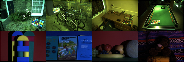
Figure 3: Images from the two benchmarks used in the experiments. Top: the SFU Color Checker Dataset; Bottom: the SFU Indoor Dataset.

IV-A Datasets and Measurement

The proposed method is evaluated on two popular benchmarking datasets [4, 22, 35] with linear images. The SFU Color Checker dataset [22, 35] contains 568 14-bits dynamic range images which all include the Macbeth Color Checker chart. The SFU Indoor dataset [4] includes more artificially-looking scenes, containing 321 images captured in 11 different controlled lighting conditions. Groudtruth of both datasets are provided. Sample images from the two datasets are shown in Fig. 3.

Following the standard procedure [6], we evenly split the data into training, validation and testing sets. We train our regressors and use the validation set to tune free parameters of the regressors. The procedure is repeated $30$ times with different random splits. The average errors are reported.

Following the prior work [4, 14, 22, 35], the accuracy of illumination estimation is measured by the angular error $\varepsilon$ between estimated illumination $I$ and groundtruth $I_{gt}$:

$$\varepsilon_{I,I_{gt}}=\arccos(\frac{I\cdot I_{gt}}{\parallel I\parallel\cdot\parallel I_{gt}\parallel}),\enspace$$

where $\cdot$ denotes the inner product between vectors, $\parallel\cdot\parallel$ is Euclidean norm.

IV-B Regressor Learning Settings

Free parameters in the aforementioned regressors need to be tuned: regularization trade-off parameter $C$, kernel coefficient $\gamma$ for the RBF kernel and insensitivity parameter $\epsilon$ in MSVR.

• For multi-output ridge regression, only trade-off parameter $C$ is chosen from $C\in 10^{(-2:1:2)}$.

• For our structured-output SVR implementation (i.e., CNN+MSVR), we choose the optimized parameters by searching in grid space where $C\in 10^{(-3:1:5)}$, $\gamma\in 10^{(-4:1:4)}$ and $\epsilon\in 10^{(-4:2:3)}$.

IV-C Comparison to State-of-the-Art

In Table I, the median, the average, and the maximum of the angular errors of state-of-the-art methods and our methods are evaluated and compared. We categorize these methods into three groups in the table: non-learning algorithms (top), camera-specific ones (middle) and learning-based ones (bottom). The best results for each metric are in bold.

The multi-output ridge regression (CNN+MRR), multi-output support vector regression (CNN+MSVR) and ridge regression (CNN+RR) are our implementations. They all share the same CNN features from the “fc₆” layer of VGG CNN. From Table I, it is evident that even a medium-depth CNN [32] coupled with SVR (CNN+SVR [6]) shows better performance than all statistics based algorithms and most of gamut based and learning based methods. Specifically, our CNN+MSVR outperforms the best non-learning based methods (Grey Pixel) on the SFU color checker and the SFU indoor datasets by decreasing the median angular error with 13.55$\%$ and 28.70$\%$ respectively. Compared to the existing camera-specific and learning based frameworks, the significant improvement of our CNN-MSVR is achieved on the SFU Indoor dataset, while our solution is comparable to the state-of-the-art on the SFU Color Checker benchmark.

The significant improvement on CNN+SVR over its direct competitor SVR can be attributed to the introduction of powerful CNN features, which demonstrates the advantages of adopting CNN features for illumination estimation. Moreover, direct comparison between CNN+SVR and CNN+MSVR substitutes our main contribution to capture inter-channel correlations by using structured-output regressors, with CNN+MSVR significantly outperforming CNN+SVR. A similar situation is observed for single-output CNN+RR and structural output model CNN+MRR on both benchmarks.

IV-D Choosing CNN Architecture, Layer, and The Regressor

TABLE II: Comparison of deep features from AlexNet and VGG CNNs.

	SFU Color Checker			SFU Indoor
	Median	Mean	Max	Median	Mean	Max
AlexNetfc6	3.60	5.00	19.91	1.68	3.59	12.96
VGGfc6	2.68	4.29	20.35	1.64	3.25	21.39

TABLE III: Comparison of deep features from “fc₆”, “fc₇”, “fc₈” layers.

	SFU Color Checker
	Median	Mean	Max
VGGfc6	2.68	4.29	20.35
VGGfc7	2.91	4.28	23.29
VGGfc8	3.10	4.56	26.26

Our best result (last row in Table I) is obtained by an optimized combination of the CNN architecture, the CNN layer and the regressor, on which evaluation experiments have been done respectively.

Firstly we choose the VGG features as default setting because VGG outperforms AlexNet on two datasets used in our experiments. Table II shows in the metric of median error and mean error, VGG_fc6+MSVR achieved 0.7$\sim$0.9 reduction on SFU Color Checker, while on SFU Indoor, this superiority seems not that distinct.

In the second step we investigate the effect of depth of feature extraction layer designed for visual recognition on illumination estimation. The deep feature has been extracted from three fully-connected layers: “fc₆”, “fc₇”, “fc₈” shown in Fig. 2. Each type of deep feature is fed into MSVR model to compare the estimation performance. In Table III, one trend is discovered: the deeper the CNN layer we adopt, the worse the performance we can achieve. One possible explanation could be that illumination estimation relies more on low-level information like edges, colors than abstract high-level knowledge for visual understanding as some synthetic examples look fragmented and contain no object or just part of it. Then, the regressor (MSVR) with the highest performance is chosen from three candidates (MSVR, MRR, RR) using the same settings, which is already analyzed in Section IV-C.

TABLE IV: Multi-output SVR training with data augmentation.

		SFU Color Checker
Method	Augmentation	Min	Median	Mean	Max
CNN+MSVR	–	–	2.68	4.29	20.35
CNN+MSVR	random patches	0.02	3.28	4.35	20.42
CNN+MSVR	regular patches	0.13	3.15	3.87	21.36

It is known that CNN can work for regression problems directly and we do one more experiments to illustrate the advantages of CNN feature with structured-output regressors over CNN model only. For the aim to expand the amount of training examples massively, two simple cropping or patching strategies are considered. Randomly cropping is to randomly crop 224$\times$224 patches from resized original image ($max(w,h)=1000$), while sliding-window patching is aimed to get 224$\times$224 clipped image patches using a square sliding window to scan the whole image region. As shown in Table IV, this two strategies suffer from over-fitting and cannot achieve competitive performance, compared to the proposed deep structured-output regression frameworks.

V Conclusions

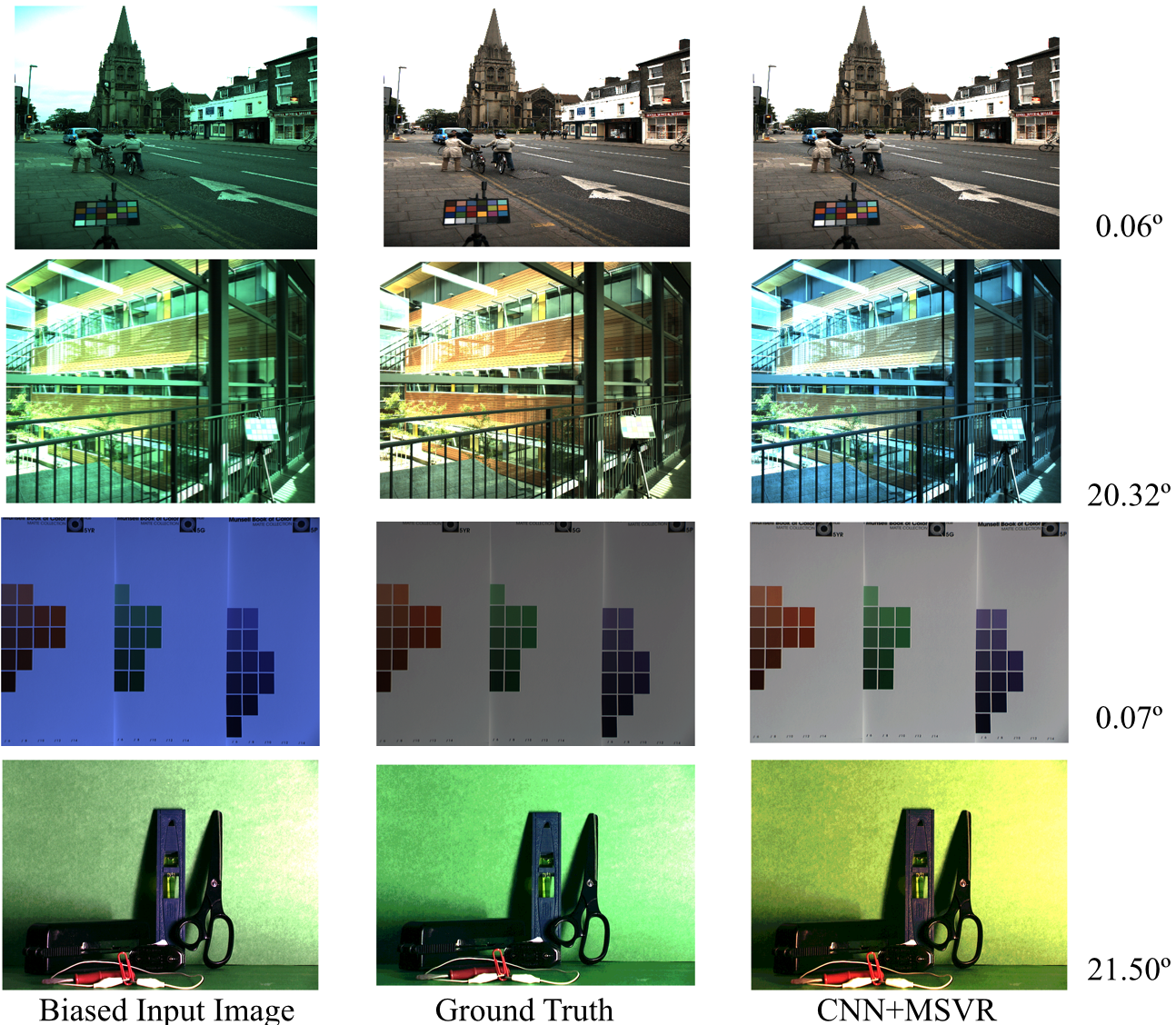
Figure 4: Results of the best and the worst cases on two datasets (first two rows: the SFU Color Checker dataset, last two rows: the SFU Indoor dataset) after applying the proposed algorithm. The angular error between corrected images and groundtruth is marked on the right hand side.

A novel method addressing the color constancy problem by structured-output regression on the values of the fully-connected layers of a convolutional neural network has been proposed. Two widely used AlexNet and VGG CNNs were compared and VGG outperformed AlexNet by a margin of around 30% in the median error. Experiments on the SFU Color Checker and Indoor Dataset benchmarks demonstrate that our method achieves competitive performance, outperforming the state of the art on the SFU indoor benchmark with an angular error of $1.64^{\circ}$.

References

- [1] O. Arandjelović. Colour invariants under a non-linear photometric camera model and their application to face recognition from video. Pattern Recognition, 45(7):2499–2509, 2012.
- [2] K. Barnard. Improvements to gamut mapping colour constancy algorithms. In Proceedings of European Conference on Computer Vision. 2000.
- [3] K. Barnard, V. Cardei, and B. Funt. A comparison of computational color constancy algorithms. i: Methodology and experiments with synthesized data. IEEE Transactions on Image Processing, 11(9):972–984, 2002.
- [4] K. Barnard, L. Martin, B. Funt, and A. Coath. A data set for color research. Color Research & Application, 27(3):147–151, 2002.
- [5] J. T. Barron. Convolutional color constancy. In Proceedings of International Conference on Computer Vision, 2015.
- [6] S. Bianco, C. Cusano, and R. Schettini. Color constancy using cnns. In Proceedings of IEEE Conference on Computer Vision and Pattern Recognition Workshops, 2015.
- [7] H. Borchani, G. Varando, C. Bielza, and P. Larrañaga. A survey on multi-output regression. Wiley Interdisciplinary Reviews: Data Mining and Knowledge Discovery, 5(5):216–233, 2015.
- [8] D. H. Brainard and B. A. Wandell. Analysis of the retinex theory of color vision. Journal of the Optical Society of America, 3(10):1651–1661, 1986.
- [9] M. H. Brill. Minimal von kries illuminant invariance. Color Research & Application, 33(4):320–323, 2008.
- [10] G. Buchsbaum. A spatial processor model for object colour perception. Journal of the Franklin institute, 310(1):1–26, 1980.
- [11] V. C. Cardei, B. Funt, and K. Barnard. White point estimation for uncalibrated images. In Proceedings of Color Imaging Conference, volume 1999, pages 97–100, 1999.
- [12] A. Chakrabarti, K. Hirakawa, and T. Zickler. Color constancy with spatio-spectral statistics. IEEE Transactions on Pattern Analysis and Machine Intelligence, 34(8):1509–1519, 2012.
- [13] K. Chen, S. Gong, T. Xiang, and C. Loy. Cumulative attribute space for age and crowd density estimation. In Proceedings of IEEE Conference on Computer Vision and Pattern Recognition, 2013.
- [14] F. Ciurea and B. Funt. A large image database for color constancy research. In Proceedings of Color Imaging Conference, 2003.
- [15] G. D. Finlayson, M. S. Drew, and B. V. Funt. Color constancy: generalized diagonal transforms suffice. Journal of the Optical Society of America, 11(11):3011–3019, 1994.
- [16] G. D. Finlayson, S. D. Hordley, and P. M. Hubel. Color by correlation: A simple, unifying framework for color constancy. IEEE Transactions on Pattern Analysis and Machine Intelligence, 23(11):1209–1221, 2001.
- [17] G. D. Finlayson and G. Schaefer. Hue that is invariant to brightness and gamma. In Proceedings of British Machine Vision Conference, 2001.
- [18] G. D. Finlayson and E. Trezzi. Shades of gray and colour constancy. In Proceedings of Color Imaging Conference, 2004.
- [19] D. A. Forsyth. A novel algorithm for color constancy. International Journal of Computer Vision, 5(1):5–35, 1990.
- [20] B. Funt, K. Barnard, and L. Martin. Is machine colour constancy good enough? In Proceedings of European Conference on Computer Vision. 1998.
- [21] B. Funt and W. Xiong. Estimating illumination chromaticity via support vector regression. In Proceedings of Color Imaging Conference, 2004.
- [22] P. V. Gehler, C. Rother, A. Blake, T. Minka, and T. Sharp. Bayesian color constancy revisited. In Proceedings of IEEE Conference on Computer Vision and Pattern Recognition, 2008.
- [23] A. Gijsenij and T. Gevers. Color constancy using natural image statistics and scene semantics. IEEE Transactions on Pattern Analysis and Machine Intelligence, 33(4):687–698, 2011.
- [24] A. Gijsenij, T. Gevers, and J. Van De Weijer. Generalized gamut mapping using image derivative structures for color constancy. International Journal of Computer Vision, 86(2-3):127–139, 2010.
- [25] A. Gijsenij, T. Gevers, and J. Van De Weijer. Computational color constancy: Survey and experiments. IEEE Transactions on Image Processing, 20(9):2475–2489, 2011.
- [26] A. Gijsenij, T. Gevers, and J. Van De Weijer. Improving color constancy by photometric edge weighting. IEEE Transactions on Pattern Analysis and Machine Intelligence, 34(5):918–929, 2012.
- [27] R. Hunt and M. Pointer. Metamerism and colour constancy. Measuring Colour, Fourth Edition, pages 117–142.
- [28] T. Joachims, T. Finley, and C.-N. J. Yu. Cutting-plane training of structural svms. Machine Learning, 77(1):27–59, 2009.
- [29] H. R. V. Joze and M. S. Drew. Exemplar-based color constancy and multiple illumination. IEEE Transactions on Pattern Analysis and Machine Intelligence, 36(5):860–873, 2014.
- [30] H. R. V. Joze, M. S. Drew, G. D. Finlayson, and P. A. T. Rey. The role of bright pixels in illumination estimation. In Proceedings of Color Imaging Conference, 2012.
- [31] K. Kavukcuoglu, P. Sermanet, Y.-L. Boureau, K. Gregor, M. Mathieu, and Y. L. Cun. Learning convolutional feature hierarchies for visual recognition. In Advances in neural information processing systems, 2010.
- [32] A. Krizhevsky, I. Sutskever, and G. E. Hinton. Imagenet classification with deep convolutional neural networks. In Advances in neural information processing systems, 2012.
- [33] D. Lee and K. N. Plataniotis. A taxonomy of color constancy and invariance algorithm. In Advances in Low-Level Color Image Processing, pages 55–94. 2014.
- [34] N. Moroney, M. D. Fairchild, R. W. Hunt, C. Li, M. R. Luo, and T. Newman. The ciecam02 color appearance model. In Proceedings of Color Imaging Conference, 2002.
- [35] L. Shi and B. Funt. Re-processed version of the gehler color constancy dataset of 568 images. Simon Fraser University, 1(2):3, 2010.
- [36] K. Simonyan and A. Zisserman. Very deep convolutional networks for large-scale image recognition. arXiv preprint arXiv:1409.1556, 2014.
- [37] A. J. Smola and B. Schölkopf. A tutorial on support vector regression. Statistics and computing, 14(3):199–222, 2004.
- [38] C. Szegedy, W. Liu, Y. Jia, P. Sermanet, S. Reed, D. Anguelov, D. Erhan, V. Vanhoucke, and A. Rabinovich. Going deeper with convolutions. In Proceedings of IEEE Conference on Computer Vision and Pattern Recognition, 2015.
- [39] J. Van De Weijer, T. Gevers, and J.-M. Geusebroek. Edge and corner detection by photometric quasi-invariants. IEEE Transactions on Pattern Analysis and Machine Intelligence, 27(4):625–630, 2005.
- [40] J. Van De Weijer, T. Gevers, and A. Gijsenij. Edge-based color constancy. IEEE Transactions on Image Processing, 16(9):2207–2214, 2007.
- [41] J. Van De Weijer, C. Schmid, and J. Verbeek. Using high-level visual information for color constancy. In Proceedings of International Conference on Computer Vision, 2007.
- [42] J. von Kries. Chromatic adaptation. Festschrift der Albrecht-Ludwigs-Universität, pages 145–158, 1902.
- [43] K.-F. Yang, S.-B. Gao, and Y.-J. Li. Efficient illuminant estimation for color constancy using grey pixels. In Proceedings of IEEE Conference on Computer Vision and Pattern Recognition, 2015.