The Partially Observable Hidden Markov Model
and its Application to Keystroke Dynamics

Abstract

The partially observable hidden Markov model is an extension of the hidden Markov Model in which the hidden state is conditioned on an independent Markov chain. This structure is motivated by the presence of discrete metadata, such as an event type, that may partially reveal the hidden state but itself emanates from a separate process. Such a scenario is encountered in keystroke dynamics whereby a user’s typing behavior is dependent on the text that is typed. Under the assumption that the user can be in either an active or passive state of typing, the keyboard key names are event types that partially reveal the hidden state due to the presence of relatively longer time intervals between words and sentences than between letters of a word. Using five public datasets, the proposed model is shown to consistently outperform other anomaly detectors, including the standard HMM, in biometric identification and verification tasks and is generally preferred over the HMM in a Monte Carlo goodness of fit test.

url]http://www.vmonaco.com

1 Introduction

The hidden Markov model (HMM), which dates back over 50 years [1], has seen numerous applications in the recognition of human behavior, such as speech [2], gesture [3], and handwriting [4]. Recent successes have leveraged the expressive power of connectionist models by combining the HMM with feed-forward deep neural networks, which are used to estimate emission probabilities [5, 6, 7]. Despite the increasing interest in sequential deep learning techniques, e.g., recurrent neural networks, HMMs remain tried-and-true for time series analyses. The popularity and endurance of the HMM can be at least partially attributed to the tractability of core problems (parameter estimation and likelihood calculation), ability to be combined with other methods, and the level of insight it provides to the data.

At least part its success can also be attributed to its flexibility, with many HMM variants having been developed for specific applications. This usually involves introducing a dependence, whether it be on time [8], previous observations [9], or a semantic context [10]. The motivation for doing so is often to better reflect the structure of the underlying problem. Although many of these variations have increased complexity and number of parameters over the standard HMM, their estimation remains tractable.

In this work, we introduce the partially observable hidden Markov model (POHMM), an extension of the HMM intended for keystroke dynamics. We are interested in modeling the temporal behavior of a user typing on a keyboard, and note that certain keyboard keys are thought to influence typing speed. Non-letter keys, such as punctuation and the Space key, indicate a greater probability of being in a passive state of typing, as opposed to an active state, since the typist often pauses between words and sentences as opposed to between letters in a word [11]. The POHMM reflects this scenario by introducing a dependency on the key names which are observed alongside the time intervals, and in this way, the keys provide a context for the time intervals.

The idea of introducing a context upon which some behavior depends is not new. Often, an observation depends not only on a latent variable but on the observations that preceded it. For example, the neighboring elements in a protein secondary structure can provide context for the element under consideration, which is thought to depend on both the previous element and a hidden state [9]; nearby phonemes can aid in the recognition of phonemes [12]; and the recognition of human activities can be achieved with greater accuracy by considering both a spatial context (e.g., where the activity occurred) and temporal context (e.g., the duration of the activity) [13].

Handwriting recognition has generally seen increased performance with models that consider the surrounding context of a handwritten character. The rationale for such an approach is that a character may be written with different style or strokes depending on its neighboring characters in the sequence. Under this assumption, the neighboring pixels or feature vectors of neighboring characters can provide additional context for the character under consideration. Alternatively, a separate model can be trained for each context in which the character appears, e.g., “t” followed by “e” versus “t” followed by “h” [10]. This same principle motivates the development of the POHMM, with the difference being that the context is provided not by the observations themselves, but by a separate sequence.

We apply the POHMM to address the problems of user identification, verification, and continuous verification, leveraging keystroke dynamics as a behavioral biometric. Each of these problems requires estimating the POHMM parameters for each individual user. Identification is performed with the maximum a posteriori (MAP) approach, choosing the model with maximum a posterior probability; verification, a binary classification problem, is achieved by using the model log-likelihood as a biometric score; and continuous verification is achieved by accumulating the scores within a sliding window over the sequence. Evaluated on five public datasets, the proposed model is shown to consistently outperform other leading anomaly detectors, including the standard HMM, in biometric identification and verification tasks and is generally preferred over the HMM in a Monte Carlo goodness of fit test.

All of the core HMM problems remain tractable for the POHMM, including parameter estimation, hidden state prediction, and likelihood calculation. However, the dependency on event types introduces many more parameters to the POHMM than its HMM counterpart. Therefore, we address the problem of parameter smoothing, which acts as a kind of regularization and avoids overfitting [14]. In doing so, we derive explicit marginal distributions, with event type marginalized out, and demonstrate the equivalence between the marginalized POHMM and the standard HMM. The marginal distributions conveniently act as a kind of backoff, or fallback, mechanism in case of missing data, a technique rooted in linguistics [15].

The rest of this article is organized as follows. Section 2 briefly describes keystroke dynamics as a behavioral biometric. Section 3 introduces the POHMM, followed by a simulation study in Section 4 and a case study of the POHMM applied to keystroke dynamics in Section 5. Section 6 reviews previous modeling efforts for latent processes with partial observability and contains a discussion. Finally, Section 7 concludes the article. The POHMM is implemented in the pohmm Python package and source code is publicly available.

2 Keystroke dynamics

Keystroke dynamics refers to the way a person types. Prominently, this includes the timings of key press and release events, where each keystroke is comprised of a press time $t_{n}$ and a duration $d_{n}$. The time interval between key presses, $\tau_{n}=t_{n}-t_{n-1}$, is of interest. Compared to random time intervals (RTIs) in which a user presses only a single key [16], key press time intervals occur between different keys and are thought to be dependent on key distance [11]. A user’s keystroke dynamics is also thought to be relatively unique to the user, which enable biometric applications, such as user identification and verification [17].

As a behavioral biometric, keystroke dynamics enables low-cost and non-intrusive user identification and verification. Keystroke dynamics-based verification can be deployed remotely, often as a second factor to username-password verification. Some of the same attributes that make keystroke dynamics attractive as a behavioral biometric also present privacy concerns [18], as there exist numerous methods of detecting keystrokes without running software on the victim’s computer. Recently, it has been demonstrated that keystrokes can be detected through a wide range of modalities including motion [19], acoustics [20], network traffic [21], and even WiFi signal distortion [22].

Due to the keyboard being one of the primary human-computer interfaces, it is also natural to consider keystroke dynamics as a modality for continuous verification in which a verification decision is made upon each key pressed throughout a session [23]. Continuous verification holds the promise of greater security, as users are verified continuously throughout a session beyond the initial login, which is considered a form of static verification. Being a sequential model, the POHMM is straightforward to use for continuous verification in addition to identification and static verification.

Keystroke time intervals emanate from a combination of physiology (e.g., age, gender, and handedness [24]), motor behavior (e.g., typing skill [11]), and higher-level cognitive processes [25], highlighting the difficulty in capturing a user’s typing behavior in a succinct model. Typing behavior generally evolves over time, with highly-practiced sequences able to be typed much quicker [26]. In biometrics, this is referred to as template aging. A user’s keystroke dynamics is also generally dependent on the typing task. For example, the time intervals observed during password entry are much different than those observed during email composition.

3 Partially observable hidden Markov model

The POHMM is intended for applications in which a sequence of event types provides context for an observed sequence of time intervals. This reasoning extends activities other than keystroke dynamics, such as email, in which a user might be more likely to take an extended break after sending an email instead of receiving an email, and programming, in which a user may fix bugs quicker than making feature additions. The events types form an independent Markov chain and are observed alongside the sequence of time intervals. This is in contrast to HMM variants where the neighboring observations themselves provide a context, such as the adjacent characters in a handwritten segment [10]. Instead, the event types are independent of the dynamics of the model.

With this structure, a distinction can be made between user behavior and task: the time intervals comprise the behavior, and the sequence of event types, (e.g., the keys pressed) comprise the task. While the time intervals reflect how the user behaves, the sequence of events characterize what the user is doing. This distinction is appropriate for keystroke dynamics, in which the aim is to capture typing behavior but not the text itself which may more appropriately modeled by linguistic analysis. Alternatively, in case the user transcribes a sequence, such as in typing a password, the task is clearly defined, i.e. the user is instructed to type a particular sequence of characters. The POHMM aims to capture the temporal behavior, which depends on the task.

3.1 Description

The HMM is a finite-state model in which observed values at time $t$ depend on an underlying latent process [2]. At the $n^{\mathrm{th}}$ time step $t_{n}$, a feature vector ${\bf x}_{n}$ is emitted and the system can be in any one of $M$ hidden states, $z_{n}$. Let ${\bf x}_{1}^{N}$ be the sequence of observed emission vectors and $z_{1}^{N}$ the sequence of hidden states, where $N$ is the total number of observations. The basic HMM is defined by the recurrence relation,

$$P\left({\bf x}_{1}^{n+1},z_{1}^{n+1}\right)=P\left({\bf x}_{1}^{n},z_{1}^{n}\right)P\left({\bf x}_{n+1}|z_{n+1}\right)P\left(z_{n+1}|z_{n}\right)\;.$$ (1)

The POHMM is an extension of the HMM in which the hidden state and emission depend on an observed independent Markov chain. Starting with the HMM axiom in Equation 1, the POHMM is derived through following assumptions:

1. An independent Markov chain of event types is given, denoted by $\Omega_{1}^{N}$.

2. The emission ${\bf x}_{n+1}$ depends on event type $\Omega_{n+1}$ in addition to $z_{n+1}$.

3. The hidden state $z_{n+1}$ depends on $\Omega_{n}$ and $\Omega_{n+1}$ in addition to $z_{n}$.

Applying the above assumptions to the HMM axiom, the conditional emission probability $P\left({\bf x}_{n+1}|z_{n+1}\right)$ becomes $P\left({\bf x}_{n+1}|z_{n+1},\Omega_{n+1}\right)$; the conditional hidden state probability $P\left(z_{n+1}|z_{n}\right)$ becomes $P\left(z_{n+1}|z_{n},\Omega_{n},\Omega_{n+1}\right)$; and the recurrence relation still holds. The complete POHMM axiom is given by the formula,

$$P\left({\bf x}_{1}^{n+1},z_{1}^{n+1}\right)=P\left({\bf x}_{1}^{n},z_{1}^{n}\right)P\left({\bf x}_{n+1}|z_{n+1},\Omega_{n+1}\right)P\left(z_{n+1}|z_{n},\Omega_{n},\Omega_{n+1}\right)$$ (2)

where $\Omega_{n}$ and $\Omega_{n+1}$ are the observed event types at times $t_{n}$ and $t_{n+1}$. The POHMM structure is shown in Figure 1.

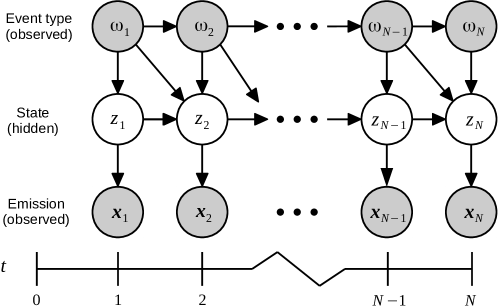
Figure 1: Partially observable hidden Markov model structure. Observed values (emission and event type) are shown in gray, hidden values (system state) are shown in white.

The event types come from a finite alphabet of size $m$. Thus, while the HMM has $M$ hidden states, a POHMM with $m$ event types has $M$ hidden states per event type, for a total of $m\times M$ unique hidden states.

The event type can be viewed as a partial indexing to a much larger state space. Each observed event type restricts the model to a particular subset of $M$ hidden states with differing probabilities of being in each hidden state, hence the partial observability. The POHMM starting and emission probabilities can be viewed as an HMM for each event type, and the POHMM transition probabilities as an HMM for each pair of event types.

To illustrate this concept, consider a POHMM with two hidden states and three event types, where $\Omega_{1}^{3}=\left[b,a,c\right]$. At each time step, the observed event type limits the system to hidden states that have been conditioned on that event type, as demonstrated in Figure 2. Beginning at time $1$, given observed event type $\Omega_{1}=b$, the system must be in one of the hidden states $\left\{1b,2b\right\}$. Event type $\Omega_{2}=a$ observed at time $2$ then restricts the possible transitions from $\left\{1b,2b\right\}$ to $\left\{1a,2a\right\}$. Generally, given any event type, the POHMM must be in one of $M$ hidden states conditioned on that event type. Section 3.6 deals with situations where the event type is missing or has not been previously observed in which case the marginal distributions (with the event type marginalized out) are used.

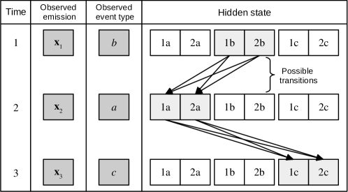
Figure 2: POHMM event types index a much larger state space. In this example, there are two hidden states and three event types. Given observed event type $b$ at time $1$, the system must be in one of the hidden states $\left\{1b,2b\right\}$. The $a$ observed at the next time step limits the possible transitions from $\left\{1b,2b\right\}$ to $\left\{1a,2a\right\}$.

The POHMM parameters are derived from the HMM. Model parameters include $\pi\left[j|\omega\right]$, the probability of starting in state $j$ given event type $\omega$, and $a\left[i,j|\psi,\omega\right]$, the probability of transitioning from state $i$ to state $j$, given event types $\psi$ and $\omega$ before and after the transition, respectively. Let $f\left(\cdot;{\bf b}\left[j|\omega\right]\right)$ be the emission distribution that depends on hidden state $j$ and event type $\omega$, where ${\bf b}\left[j|\omega\right]$ parametrizes density function $f\left(\cdot\right)$. The complete set of parameters is denoted by $\theta=\left\{\pi,a,{\bf b}\right\}$, where $a$ is the $m^{2}M^{2}$ transition matrix. While the total number of parameters in the HMM is $M+M^{2}+MK$, where $K$ is the number of free parameters in the emission distribution, the POHMM contains $mM+m^{2}M^{2}+mMK$ parameters. After accounting for normalization constraints, the degrees of freedom (dof) is $m\left(M-1\right)+m^{2}M\left(M-1\right)+mMK$.

Marginal distributions, in which the event type is marginalized out, are also defined. Let $\pi\left[j\right]$ and $f\left(\cdot;{\bf b}\left[j\right]\right)$ be the marginalized starting and emission probabilities, respectively. Similarly, the parameters $a\left[i,j|\omega\right]$, $a\left[i,j|\psi\right]$, and $a\left[i,j\right]$ are defined as the transition probabilities after marginalizing out the first, second, and both event types, respectively. The POHMM marginal distributions are exactly equal to the corresponding HMM that ignores the event types. This ensures that the POHMM is no worse than the HMM in case the event types provide little or no information as to the process being modeled. Computation of POHMM marginal distributions is covered in Section 3.6 and simulation results demonstrating this equivalence are in Section 4.

It may seem that POHMM parameter estimation becomes intractable, as the number of possible transitions between hidden states increases by a factor of $m^{2}$ over the HMM and all other parameters by a factor of $m$. In fact, all of the algorithms used for the POHMM are natural extensions of those used for the HMM: the POHMM parameters and variables are adapted from the HMM by introducing the dependence on event types, and parameter estimation and likelihood calculation follow the same basic derivations as those for the HMM. POHMM parameter estimation remains linearly bounded in the number of observations, similar to the HMM, performed through a modification of the Baum-Welch (BW) algorithm. The convergence property of the modified BW algorithm is demonstrated analytically in Section 3.4 and empirically in Section 4. The rest of this section addresses the three main problems of the POHMM, taken analogously as the three main problems of the HMM:

1. Determine $P({\bf x}_{1}^{N}|\Omega_{1}^{N},\theta)$, the likelihood of an emission sequence given the model parameters and the observed event types.

2. Determine $z_{1}^{N}$, the maximum likelihood sequence of hidden states, given the emissions ${\bf x}_{1}^{N}$ and event types $\Omega_{1}^{N}$.

3. Determine $\arg\max_{\theta\in\Theta}P({\bf x}_{1}^{N}|\Omega_{1}^{N},\theta)$, the maximum likelihood parameters $\theta$ for observed emission sequence ${\bf x}_{1}^{N}$, given the event type sequence.

The first and third problems are necessary for identifying and verifying users in biometric applications, while the second problem is useful for understanding user behavior. The rest of this section reviews the solutions to each of these problems and other aspects of parameter estimation, including parameter initialization and smoothing.

3.2 Model likelihood

Since we assume $\Omega_{1}^{N}$ is given, it does not have a prior distribution. Therefore, we consider only the likelihood of an emission sequence given the model parameters $\theta$ and the observed event type sequence $\Omega_{1}^{N}$, denoted by $P({\bf x}_{1}^{N}|\Omega_{1}^{N})$, leaving the joint model likelihood $P({\bf x}_{1}^{N},\Omega_{1}^{N})$ as an item for future work.

In the HMM, $P({\bf x}_{1}^{N})$ can be computed efficiently by the forward procedure which defines a recurrence beginning at the start of the sequence. This procedure differs slightly for the POHMM due to the dependence on event types. Notably, the starting, transition, and emission parameters are all conditioned on the given event type.

Let $\alpha_{n}\left[z_{n},\Omega_{n}\right]\equiv P\left({\bf x}_{1}^{n},z_{n}|\Omega_{n}\right)$, i.e., the joint probability of emission subsequence ${\bf x}_{1}^{n}$ and hidden state $z_{n}$, given event type $\Omega_{n}$. Then, by the POHMM axiom (Equation 2), $\alpha_{n}\left[z_{n},\Omega_{n}\right]$ can be computed recursively by the formula,

$$\alpha_{n+1}\left[z_{n+1},\Omega_{n+1}\right] = P\left({\bf x}_{n+1}|z_{n+1},\Omega_{n+1}\right)$$

$$\times\sum_{z_{n}}P\left(z_{n+1}|z_{n},\Omega_{n},\Omega_{n+1}\right)\alpha_{n}\left[z_{n},\Omega_{n}\right]$$

$$\alpha_{1}\left[z_{1},\Omega_{1}\right] = P\left({\bf x}_{1}|z_{1},\Omega_{1}\right)P\left(z_{1}|\Omega_{1}\right)$$ (4)

where Equation 4 provides the initial condition. The modified forward algorithm is obtained by substituting the model parameters into Equations 3.2 and 4, where

$$\pi\left[j|\omega\right] \equiv P\left(z_{1}=j|\Omega_{1}=\omega\right)$$ (5)

$$f({\bf x}_{n};{\bf b}\left[j,\omega\right]) \equiv P\left({\bf x}_{n}|z_{n}=j,\Omega_{n}=\omega\right)$$ (6)

$$a\left[i,j|\psi,\omega\right] \equiv P\left(z_{n+1}=j|z_{n}=i,\Omega_{n}=\psi,\Omega_{n+1}=\omega\right)$$ (7)

and $\alpha_{n}\left[j,\omega\right]$ is the sequence obtained after substituting the model parameters. The model likelihood is easily computed upon termination, since $P({\bf x}_{1}^{N}|\Omega_{1}^{N})=\sum_{j=1}^{M}\alpha_{N}\left[j,\omega\right]$ where $\omega=\Omega_{N}$.

A modified backward procedure is similarly defined through a backwards recurrence. Let $\beta_{n}\left[z_{n},\Omega_{n}\right]\equiv P\left({\bf x}_{n+1}^{N}|z_{n},\Omega_{n}\right)$. Then under the POHMM axiom,

$$\beta_{n}\left[z_{n},\Omega_{n}\right] = \sum_{z_{n+1}}P\left({\bf x}_{n+1}|z_{n+1},\Omega_{n+1}\right)$$

$$\quad\times P\left(z_{n+1}|z_{n},\Omega_{n},\Omega_{n+1}\right)\beta_{n+1}\left[z_{n+1},\Omega_{n+1}\right]$$

$$\beta_{N}\left[z_{N},\Omega_{N}\right] = 1\;.$$ (9)

where $\beta_{n}\left[j,\omega\right]$ is the sequence obtained after making the same substitutions.

Note that at each $n$, $\alpha_{n}\left[j,\omega\right]$ and $\beta_{n}\left[j,\omega\right]$ need only be computed for the observed $\omega=\Omega_{n}$, i.e., we don’t care about event types $\omega\neq\Omega_{n}$. Therefore, only the hidden states (and not the event types) are enumerated in Equations 3.2 and 3.2 at each time step. Like the HMM, the modified forward and backward algorithms have time complexity $O(M^{2}N)$ and can be stored in a $N\times M$ matrix.

3.3 Hidden state prediction

The maximum likelihood sequence of hidden states is efficiently computed using the event type-dependent forward and backward variables defined above. First, let the POHMM forward-backward variable $\gamma_{n}\left[z_{n},\Omega_{n}\right]\equiv P\left(z_{n}|\Omega_{n},{\bf x}_{1}^{N}\right)$, i.e., the posterior probability of hidden state $z_{n}$, given event type $\Omega_{n}$ and the emission sequence ${\bf x}_{1}^{N}$. Let $\gamma_{n}\left[j,\omega\right]$ be the estimate obtained using the model parameters, making the same substitutions as above. Then $\gamma_{n}\left[j,\omega\right]$ is straightforward to compute using the forward and backward variables, given by

$$\gamma_{n}\left[j,\omega\right] = \frac{\alpha_{n}\left[j|\omega\right]\beta_{n}\left[j|\omega\right]}{P({\bf x}_{1}^{N}|\Omega_{1}^{N})}$$

$$= \frac{\alpha_{n}\left[j|\omega\right]\beta_{n}\left[j|\omega\right]}{\sum_{i=1}^{M}\alpha_{n}\left[i|\omega\right]\beta_{n}\left[i|\omega\right]}$$

where $\omega=\Omega_{n}$. The sequence of maximum likelihood hidden states is taken as,

$$z_{n}=\mbox{arg max}_{1\leq j\leq M}\gamma_{n}\left[j,\omega\right]\;.$$ (11)

Similar to $\alpha_{n}\left[j|\omega\right]$ and $\beta_{n}\left[j|\omega\right]$, $\gamma_{n}\left[j,\omega\right]$ can be stored in a $N\times M$ matrix and takes $O\left(M^{2}N\right)$ time to compute. This is due to the fact that the event types are not enumerated at each step; the dependency on the event type propagates all the way to the re-estimated parameters, defined below.

3.4 Parameter estimation

1. Initialization
   Choose initial parameters $\theta_{o}$ and let $\theta\leftarrow\theta_{o}$.

2. Expectation
   Use $\theta$, ${\bf x}_{1}^{N}$, $\Omega_{1}^{N}$ to compute $\alpha_{n}\left[j|\omega\right]$, $\beta_{n}\left[j|\omega\right],$ $\gamma_{n}\left[j,\omega\right]$, $\xi_{n}\left[i,j|\psi,\omega\right]$.

3. Maximization
   Update $\theta$ using the re-estimation formulae (Eqs. 12, 14, 15) to get $\dot{\theta}=\left\{\dot{\pi},\dot{a},\dot{{\bf b}}\right\}$.

4. Regularization
   Calculate marginal distributions and apply parameter smoothing formulae.

5. Termination
   If $\ln P\left({\bf x}_{1}^{N}|\Omega_{1}^{N},\dot{\theta}\right)-\ln P\left({\bf x}_{1}^{N}|\Omega_{1}^{N},\theta\right)<\epsilon$, stop; else let $\theta\leftarrow\dot{\theta}$ and go to step 2.

Algorithm 1 Modified Baum-Welch for POHMM parameter estimation.

Parameter estimation is performed iteratively, updating the starting, transition, and emission parameters using the current model parameters and observed sequences. In each iteration of the modified Baum-Welch algorithm, summarized in Algorithm 1, the model parameters are re-estimated using the POHMM forward, backward, and forward-backward variables. Parameters are set to initial values before the first iteration, and convergence is reached upon a loglikelihood increase of less than $\epsilon$.

3.4.1 Starting parameters

Using the modified forward-backward variable given by Equation 3.3, the re-estimated POHMM starting probabilities are obtained directly by

$$\dot{\pi}\left[j|\omega\right]=\gamma_{1}\left[j|\omega\right]$$ (12)

where $\omega=\Omega_{1}$ and re-estimated parameters are denoted by a dot. Generally, it may not be possible to estimate $\dot{\pi}\left[j|\omega\right]$ for many $\omega$ due to there only being one $\Omega_{1}$ (or several $\Omega_{1}$ for multiple observation sequences). Parameter smoothing, introduced in Section 3.7, addresses this issue of missing and infrequent observations.

3.4.2 Transition parameters

In contrast to the HMM, which has $M^{2}$ transition probabilities, there are $m^{2}M^{2}$ unique transition probabilities in the POHMM. Let $\xi_{n}\left[z_{n},z_{n+1}|\Omega_{n},\Omega_{n+1}\right]\equiv P\left(z_{n+1}|z_{n},\Omega_{n},\Omega_{n+1},{\bf x}_{1}^{N}\right)$, i.e., the probability of transitioning from state $z_{n}$ to $z_{n+1}$, given event types $\Omega_{n}$ and $\Omega_{n+1}$ as well as the emission sequence. Substituting the forward and backward variable estimates based on model parameters, this becomes $\xi_{n}\left[i,j|\psi,\omega\right]$, given by

$$\xi_{n}\left[i,j|\psi,\omega\right]=\frac{\alpha_{n}\left[i,\omega\right]a\left[i,j|\psi,\omega\right]f\left({\bf x}_{n+1};{\bf b}\left[j|\omega\right]\right)\beta_{n}\left[j|\omega\right]}{P({\bf x}_{1}^{N}|\Omega_{1}^{N})}\;.$$ (13)

for $1\leq n\leq N-1$, $\psi=\Omega_{n}$ and $\omega=\Omega_{n+1}$. The updated transition parameters are then calculated by

$$\dot{a}\left[i,j|\psi,\omega\right]=\frac{\sum_{n=1}^{N-1}\xi_{n}\left[i,j|\psi,\omega\right]\delta\left(\psi,\Omega_{n}\right)\delta\left(\omega,\Omega_{n+1}\right)}{\sum_{n=1}^{N-1}\gamma_{n}\left[i|\psi\right]\delta\left(\psi,\Omega_{n}\right)\delta\left(\omega,\Omega_{n+1}\right)}$$ (14)

where $\delta\left(\omega,\Omega_{n}\right)=1$ if $\omega=\Omega_{n}$ and 0 otherwise. Note that $\dot{a}\left[i,j|\psi,\omega\right]$ depends only on the transitions between event types $\psi$ and $\omega$ in $\Omega_{1}^{N}$, i.e., where $\Omega_{n}=\psi$ and $\Omega_{n+1}=\omega$, as the summand in the numerator equals $0$ otherwise. As a result, the updated transition probabilities can be computed in $O(M^{2}N)$ time, the same as the HMM, despite there being $m^{2}M^{2}$ unique transitions.

3.4.3 Emission parameters

For each hidden state and event type, the emission distribution parameters are re-estimated through the optimization problem,

$$\dot{{\bf b}}\left[j|\omega\right]=\arg\max_{{\bf b}\in\mathcal{B}}\sum_{n=1}^{N}\gamma_{n}\left[j|\omega\right]\ln f\left({\bf x}_{n};{\bf b}\right)\delta\left(\omega,\Omega_{n}\right)\;.$$ (15)

Closed-form expressions exist for a variety of emission distributions. In this work, we use the log-normal density for time intervals. The log-normal has previously been demonstrated as a strong candidate for modeling keystroke time intervals, which resemble a heavy-tailed distribution [27]. The log-normal density is given by

$$f(x;\eta,\rho)=\frac{1}{x\rho\sqrt{2\pi}}\exp\left[\frac{-\left(\ln x-\eta\right)^{2}}{2\rho^{2}}\right]$$ (16)

where $\eta$ and $\rho$ are the log-mean and log-standard deviation, respectively. The emission parameter re-estimates are given by

$${\bf\dot{\eta}}\left[j|\omega\right]=\frac{\sum_{n=1}^{N}\gamma_{n}\left[j|\omega\right]\ln\tau_{n}\delta\left(\omega,\Omega_{n}\right)}{\sum_{n=1}^{N}\gamma_{n}\left[j|\omega\right]\delta\left(\psi,\Omega_{n}\right)}$$ (17)

and

$${\bf\dot{\rho}}^{2}\left[j|\omega\right]=\frac{\sum_{n=1}^{N}\gamma_{n}\left[j|\omega\right](\ln\tau_{n}-\dot{\eta}_{j|\omega})^{2}\delta\left(\omega,\Omega_{n}\right)}{\sum_{n=1}^{N}\gamma_{n}\left[j|\omega\right]\delta\left(\psi,\Omega_{n}\right)}$$ (18)

for hidden state $j$, given event type $\omega$. Note that the estimates for ${\bf\dot{\eta}}\left[j|\omega\right]$ and ${\bf\dot{\rho}}\left[j|\omega\right]$ depend only on the elements of $\gamma_{n}\left[j|\omega\right]$ where $\Omega_{n}=\omega$.

3.4.4 Convergence properties

The modified Baum-Welch algorithm for POHMM parameter estimation (Algorithm 1) relies on the principles of expectation maximization (EM) and is guaranteed to converge to a local maximum. The re-estimation formula (Equations 12, 14, and 15) are derived from inserting the model parameters from two successive iterations, $\theta$ and $\dot{\theta}$, into Baum’s auxiliary function, $Q\left(\theta,\dot{\theta}\right)$, and maximizing $Q\left(\theta,\dot{\theta}\right)$ with respect to the updated parameters. Convergence properties are evaluated empirically in Section 4, and B contains a proof of convergence, which follows that of the HMM.

3.5 Parameter initialization

Parameter estimation begins with parameter initialization, which plays an important role in the BW algorithm and may ultimately determine the quality of the estimated model since EM guarantees only locally maximum likelihood estimates. This work uses an observation-based parameter initialization procedure that ensures reproducible parameter estimates, as opposed to random initialization. The starting and transition probabilities are simply initialized as

$$\pi\left[j|\omega\right] = \frac{1}{M}$$ (19)

$$a\left[i,j|\psi,\omega\right] = \frac{1}{M}$$ (20)

for all $i$, $j$, $\psi$, and $\omega$. This reflects maximum entropy, i.e., uniform distribution, in the absence of any starting or transition priors.

Next, the emission distribution parameters are initialized. The strategy proposed here is to initialize parameters in such a way that there is a correspondence between hidden states from two different models. That is, for any two models with $M=2$, hidden state $j=1$ corresponds to the active state and $j=2$ corresponds to the passive state. Using a log-normal emission distribution, this is accomplished by spreading the log-mean initial parameters. Let

$${\bf\eta}\left[\omega\right]=\frac{\sum_{n=1}^{N}\ln{\bf x}_{n}\delta\left(\omega,\Omega_{n}\right)}{\sum_{n=1}^{N}\delta\left(\omega,\Omega_{n}\right)}$$ (21)

and

$$\rho^{2}\left[\omega\right]=\frac{\sum_{n=1}^{N}(\ln{\bf x}_{n}-\eta\left[\omega\right])^{2}\delta\left(\omega,\Omega_{n}\right)}{\sum_{n=1}^{N}\delta\left(\omega,\Omega_{n}\right)}$$ (22)

be the observed log-mean and log-variance for event type $\omega$. The model parameters are then initialized as

$${\bf\eta}\left[j|\omega\right]=\eta\left[\omega\right]+\left(\frac{2h\left(j-1\right)}{M-1}-h\right)\rho\left[\omega\right]$$ (23)

and

$$\rho^{2}\left[j|\omega\right]=\rho^{2}\left[\omega\right]$$ (24)

for $1\leq j\leq M$, where $h$ is a bandwidth parameter. Using $h=2,$ initial states are spread over the interval $\left[\eta\left[\omega\right]-2\rho\left[\omega\right],\eta\left[\omega\right]+2\rho\left[\omega\right]\right]$, i.e., 2 log-standard deviations around the log-mean. This ensures that $j=1$ corresponds to the state with the smaller log-mean, i.e., the active state.

3.6 Marginal distributions

When computing the likelihood of a novel sequence, it is possible that some event types were not encountered during parameter estimation. This situation arises when event types correspond to key names of freely-typed text and novel key sequences are observed during testing. A fallback mechanism (sometimes referred to as a “backoff” model) is typically employed to handle missing or sparse data, such as that used linguistics [15]. In order for the POHMM to handle missing or novel event types during likelihood calculation, the marginal distributions are used. This creates a two-level fallback hierarchy in which missing or novel event types fall back to the distribution in which the event type is marginalized out.

Note also that while we assume $\Omega_{1}^{N}$ is given (i.e., has no prior), the individual $\Omega_{n}$ do have a prior defined by their occurrence in $\Omega_{1}^{N}$. It is this feature that enables the event type to be marginalized out to obtain the equivalent HMM. Let the probability of event type $\omega$ at time $t_{1}$ be $\pi\left[\omega\right]$, and the probability of transitioning from event type $\psi$ to $\omega$ be denoted by $a\left[\psi,\omega\right]$. Both can be computed directly from the event type sequence $\Omega_{1}^{N}$, which is assumed to be a first-order Markov chain. The marginal $\pi\left[j\right]$ is the probability of starting in hidden state $j$ in which the event type has been marginalized out,

$$\pi\left[j\right]=\sum_{\omega\in\Omega}\pi\left[j|\omega\right]\pi\left[\omega\right]$$ (25)

where $\Omega$ is the set of unique event types in $\Omega_{1}^{N}$.

Marginal transition probabilities are also be defined. Let $a\left[i,j|\psi\right]$ be the probability of transitioning from hidden state $i$ to hidden state $j$, given event type $\psi$ while in hidden state $i$. The second event type for hidden state $j$ has been marginalized out. This probability is given by

$$a\left[i,j|\psi\right]=\sum_{\omega\in\Omega}a\left[i,j|\psi,\omega\right]a\left[\psi,\omega\right]\;.$$ (26)

The marginal probability $a\left[i,j|\omega\right]$ is defined similarly by

$$a\left[i,j|\omega\right]=\frac{\sum_{\psi\in\Omega}a\left[i,j|\psi,\omega\right]a\left[\psi,\omega\right]}{\sum_{\psi\in\Omega}a\left[\psi,\omega\right]}\;.$$ (27)

Finally, the marginal $a\left[i,j\right]$ is the probability of transitioning from $i$ to $j$,

$$a\left[i,j\right]=\frac{1}{m}\sum_{\psi\in\Omega}\sum_{\omega\in\Omega}a\left[i,j|\psi,\omega\right]a\left[\psi,\omega\right]\;.$$ (28)

No denominator is needed in Equation 26 since the normalization constraints of both transition matrices carry over to the left-hand side. Equation 28 is normalized by $\frac{1}{m}$ since $\sum_{\psi\in\Omega}\sum_{\omega\in\Omega}a\left[\psi,\omega\right]=m$.

The marginal emission distribution is a convex combination of the emission distributions conditioned on each of the event types. For normal and log-normal emissions, the marginal emission is simply a mixture of normals or log-normals, respectively. Let $\eta\left[j\right]$ and $\rho^{2}\left[j\right]$ be the log-mean and log-variance of the marginal distribution for hidden state $j$. The marginal log-mean is a weighted sum of the conditional distributions, given by

$$\eta\left[j\right]=\sum_{\omega\in\Omega}\Pi\left[\omega\right]\mu\left[j|\omega\right]$$ (29)

where $\Pi\left[\omega\right]$ is the stationary probability of event type $\omega$. This can be calculated directly from the event type sequence $\Omega_{1}^{N}$,

$$\Pi\left[\omega\right]=\frac{1}{N}\sum_{n=1}^{N}\delta\left(\omega,\Omega_{n}\right)\;.$$ (30)

Similarly, the marginal log-variance is a mixture of log-normals given by

$$\rho^{2}\left[j\right]=\sum_{\omega\in\Omega}\Pi\left[\omega\right]\left[\left(\eta\left[j|\omega\right]-\eta\left[j\right]\right)^{2}+\rho^{2}\left[j|\omega\right]\right]\;.$$ (31)

Marginalized distribution parameters for normal emission is exactly the same.

3.7 Parameter smoothing

HMMs with many hidden states (and parametric models in general) are plagued by overfitting and poor generalization, especially when the sample size is small. This has to due with there being a high dof in the model compared to the number of observations. Previous attempts at HMM parameter smoothing have pushed the emission and transition parameters towards a higher entropy distribution [14] or borrowed the shape of the emission PDF from states that appear in a similar context [12]. Instead, our parameter smoothing approach uses the marginal distributions, which can be estimated with higher confidence due to there being more observations, to eliminate the sparseness in the event type-dependent parameters. Note that parameter smoothing goes hand-in-hand with context-dependent models, at least in part due to the curse of dimensionality which is introduced by the context dependence [12].

The purpose of parameter smoothing is twofold. First, it acts as a kind of regularization to avoid overfitting, a problem often encountered when there is a large number of parameters and small number of observations. Second, parameter smoothing provides superior estimates in case of missing or infrequent data. For motivation, consider a keystroke sequence of length $N$. Including English letters and the Space key, there are at most $27$ unique keys and $729$ unique digrams (subsequences of length 2). Most of these will rarely, or never, be observed in a sequence of English text. Parameter smoothing addresses this issue by re-estimating the parameters that depend on low-frequency observations using a mixture of the marginal distribution. The effect is to bias parameters that depend on event types with low frequency toward the marginals, for which there exist more observations and higher confidence, while parameters that depend on event types with high frequency will remain unchanged.

Smoothing weights for the starting and emission parameters are defined as

$$w_{\omega}=1-\frac{1}{1+f\left(\omega\right)}$$ (32)

where $f(\omega)=\sum_{t=1}^{N}\delta\left(\omega,\Omega_{n}\right)$ is the frequency of event type $\omega$ in the sequence $\Omega_{1}^{N}$. The POHMM starting probabilities are then smoothed by

$$\tilde{\pi}\left[j|\omega\right]=w_{\omega}\pi\left[j|\omega\right]+\left(1-w_{\omega}\right)\pi\left[j\right]$$ (33)

where smoothed parameter estimates denoted by a tilde, and emission parameters are smoothed by

$$\tilde{{\bf b}}\left[j|\omega\right]=w_{\omega}{\bf b}\left[j|\omega\right]+\left(1-w_{\omega}\right){\bf b}\left[j\right]\;.$$ (34)

As $N$ increases, event type frequencies increase and the effect of parameter smoothing is diminished, while parameters conditioned on infrequent or missing event types are biased toward the marginal. This ensures that the conditional parameters remain asymptotically unbiased as $N\rightarrow\infty$.

The smoothing weights for transition probabilities follow similar formulae. Let $f\left(\psi,\omega\right)=\sum_{t=1}^{N-1}\delta\left(\psi,\Omega_{n}\right)\delta\left(\omega,\Omega_{n+1}\right)$, i.e., the frequency of event type $\psi$ followed by $\omega$ in the sequence $\Omega_{1}^{N}$. Weights for the conditional and marginal transition probabilities are defined as

$$w_{\psi} = \frac{1}{f\left(\psi,\omega\right)+f\left(\omega\right)}$$

$$w_{\omega} = \frac{1}{f\left(\psi,\omega\right)+f\left(\psi\right)}$$

$$w_{\psi,\omega} = 1-\left(w_{\psi}+w_{\omega}\right)$$

$$w = 0$$ (35)

where $w_{\psi,\omega}+w_{\psi}+w_{\omega}+w=1$. The smoothed transition matrix is given by

$$\tilde{a}\left[i,j|\psi,\omega\right]=w_{\psi,\omega}a\left[i,j|\psi,\omega\right]+w_{\psi}a\left[i,j|\psi\right]+w_{\omega}a\left[i,j|\omega\right]+wa\left[i,j\right]\;.$$ (36)

In this strategy, the weight for the marginal $a\left[i,j\right]$ is 0, although in other weighting schemes, $w$ could be non-zero.

4 Simulation study

It is important for statistical models and their implementations to be consistent. This requires that parameter estimation be both convergent and asymptotically unbiased. The POHMM algorithms include the parameter estimation procedure and equations, and the implementation consists of the POHMM algorithms expressed in a programming language. While consistency of the POHMM algorithms is theoretically guaranteed (proof in B), consistency of the POHMM implementation under several different scenarios is validated in this section using computational methods.

First, a model is initialized with parameters $\theta_{o}$. From this model, $S$ samples are generated, each containing $N$ time intervals. For each sample, the best-estimate parameters $\hat{\theta}$ are computed using the modified BW algorithm (Algorithm 1). Let $\hat{\theta}_{N}$ be the parameters determined by the modified BW algorithm for an observed sequence of length $N$ generated from a POHMM with true parameters $\theta_{o}$. Consistency requires that

$$\lim_{N\to\infty}\frac{|\hat{\theta}_{N}-\theta_{o}|}{\max_{\hat{\theta}}|\hat{\theta}_{N}-\theta_{o}|}={\bf 0}$$ (37)

insensitive to the choice of $\theta_{o}$. As $N$ increases, parameter estimation should be able to recover the true model parameters from the observed data. Four different scenarios are considered:

1. Train a POHMM (without smoothing) on POHMM-generated data.

2. Train a POHMM (with smoothing) on POHMM-generated data.

3. Train a POHMM (without smoothing) using emissions generated from an HMM and random event types.

4. Train an HMM using emissions from a POHMM (ignore event types).

Convergence is theoretically guaranteed for scenarios 1 and 2. The first scenario tests the POHMM implementation without parameter smoothing and should yield unbiased estimates. Scenario 2 evaluates the POHMM implementation with parameter smoothing, whose effect diminishes as $N$ increases. Consequently, the smoothed POHMM estimates approach that of the unsmoothed POHMM, and results should also indicate consistency.

Scenario 3 is a POHMM trained on an HMM, and scenario 4 is an HMM trained on a POHMM. In scenario 3, the underlying process is an HMM with the same number of hidden states as the POHMM, and the observed event types are completely decorrelated from the HMM. As a result, the event types do not partially reveal the hidden state. In this case, the POHMM marginal distributions, in which the event type is marginalized out, should converge to the HMM. Finally, scenario 4 simply demonstrates the inability of the HMM to capture the dependence on event types, and results should indicate biased estimates.

For scenarios 1, 2 and 4, a POHMM with 3 event types and 2 hidden states is initialized to generate the training data. The emission distribution is a univariate Gaussian with parameters chosen to be comparable to human key-press time intervals, and transition probabilities are uniformly distributed. The emission and event type sequences are sampled from the POHMM and used to fit the model. In scenario 3, an HMM generates the emission sequence ${\bf x}_{1}^{N}$, and the event type sequence $\Omega_{1}^{N}$ is chosen randomly from the set of 3 event types, reflecting no dependence on event types. In this case, only the POHMM marginal distribution parameter residuals are evaluated, as these should approximate the underlying HMM. For each value of $N$ in each scenario, 400 length-$N$ samples are generated and used to train the corresponding model.

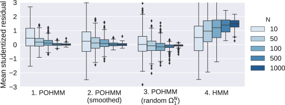
(a) Studentized emission residuals.

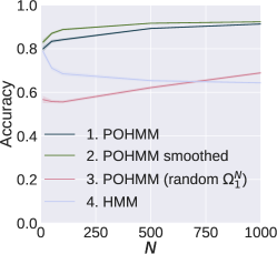
(b) Hidden state classification accuracy.

Figure 3: Simulation study results. In 1 and 2, a POHMM is trained on data generated from a POHMM; in 3, a POHMM is trained on data generated from an HMM (using random event types); in 4, an HMM is trained on data generated from a POHMM (ignoring event types).

Figure 3a contains the mean studentized residuals for emission parameters of each model, and Figure 3b shows the hidden state classification accuracies (where chance accuracy is $\frac{1}{2^{N}}$). Both the unsmoothed and smoothed POHMM residuals tend toward 0 as $N$ increases, indicating consistency. The marginal residuals for the POHMM with random event types also appear unbiased, an indication that the POHMM marginals, in which the event type is marginalized out, are asymptotically equivalent to the HMM. Finally, the HMM residuals, when trained on data generated from a POHMM, appear biased as expected when the event types are ignored. Similar results in all scenarios are seen for the transition probability residuals (not shown), and we confirmed that these results are insensitive to the choice of $\theta_{o}$.

5 Case study: keystroke dynamics

Five publicly-available keystroke datasets are analyzed in this work, summarized in Table 1. We categorize the input type as follows:

• Fixed-text: The keystrokes exactly follow a relatively short predefined sequence, e.g., passwords and phone numbers.

• Constrained-text: The keystrokes roughly follow a predefined sequence, e.g., case-insensitive passphrases and transcriptions. Some massively open online course (MOOC) providers require the student to copy several sentences for the purpose of keystroke dynamics-based verification [28].

• Free-text: The keystrokes do not follow a predefined sequence, e.g., responding to an open-ended question in an online exam.

The password, keypad, and mobile datasets contain short fixed-text input in which all the users in each dataset typed the same 10-character string followed by the Enter key: “.tie5Roanl” for the password dataset [29] and “9141937761” for the keypad [30] and mobile datasets [31]. Samples that contained errors or more than 11 keystrokes were discarded. The password dataset was collected on a laptop keyboard equipped with a high-resolution clock (estimated resolution to within ±200 μs [32]), while the timestamps in all other datasets were recorded with millisecond resolution (see discussion in Section 2 on timestamp resolution). The keypad dataset used only the 10-digit numeric keypad located on the right side a standard desktop keyboard, and the mobile dataset used an Android touchscreen keypad with similar layout. In addition to timestamps, the mobile dataset contains accelerometer, gyroscope, screen location, and pressure sensor features measured on each key press and release.

Table 1: Keystroke dataset summary. Columns 4-7 indicate: number of users, samples per user, keystrokes per sample, and $\bar{\tau}$=mean press-press latency (ms).

Dataset	Source	Category	Users	Samples/user	Keys/sample	$\bar{\tau}$ (ms)
Password	[29]	Short fixed	51	400	11	249
Keypad	[30]	Short fixed	30	20	11	376
Mobile	[31]	Short fixed	51	20	11	366
Fable	[33]	Long constrained	60	4	100	264
Essay	[34]	Long free	55	6	500	284

The fable dataset contains long constrained-text input from 60 users who each copied 4 different fables or nursery rhymes [33, 34]. Since mistakes were permitted, the keystrokes for each copy task varied, unlike the short fixed-text datasets above. The essay dataset contains long free-text input from 55 users who each answered 6 essay-style questions as part of a class exercise [34]. Both the fable and essay datasets were collected on standard desktop and laptop keyboards. For this work, the fable samples were truncated to each contain exactly 100 keystrokes and the essay samples to each contain exactly 500 keystrokes.

Each keystroke event contains two timing features,

$$\tau_{n} = t_{n}^{P}-t_{n-1}^{P}$$ (38)

$$d_{n} = t_{n}^{R}-t_{n}^{P}$$ (39)

where $t_{n}^{P}$ and $t_{n}^{R}$ are the press and release timestamps of the $n^{th}$ keystroke, respectively; $\tau_{n}$ is the press-press time interval and $d_{n}$ is the key-hold duration. Note that other timing features, such as release-release and release-press intervals, can be calculated by a linear combination of the above two features.

Each user’s keystroke dynamics are modeled by a POHMM with log-normal emission and two hidden states, all conditioned on the keyboard keys as the observed event types. A two-state model is the simplest model of non-homogeneous behavior, as one state implies a sequence of independent and identically distributed (i.i.d.) observations. The two hidden states correspond to the active and passive states of the user, in which relatively longer time intervals are observed in the passive state. Given the hidden state and the observed event type, the keystroke time intervals $\tau_{n}$ and $d_{n}$ are each modeled by a log-normal distribution (Equation 16), where $\eta\left[j|\omega\right]$ and $\rho\left[j|\omega\right]$ are the log-mean and log-standard deviation, respectively, in hidden state $j$ given observed key $\omega$.

The POHMM parameters are determined using Algorithm 1, and convergence is achieved after a loglikelihood increase less than $10^{-6}$ or 1000 iterations, whichever is reached first. As an example, the marginal key-press time interval distributions for each hidden state are shown in Figure 4 for two randomly selected samples. The passive state in the free-text model has a heavier tail than the fixed-text, while the active state distributions in both models are comparable. The rest of this section presents experimental results for a goodness of fit test, identification, verification, and continuous verification. Source code to reproduce the experiments in this article is available.

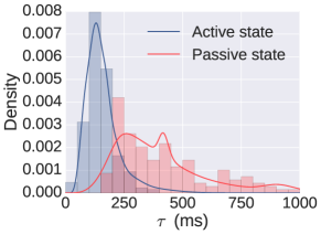
(a) Fixed-text

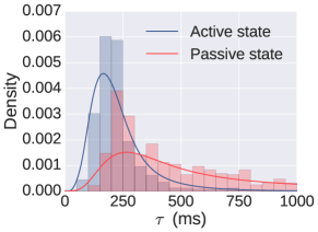
(b) Free-text

Figure 4: POHMM marginal distributions showing a separation between active and passive typing states. The marginal distributions are mixtures of log-normals conditioned on the key names. Histograms show the empirical time interval distributions in each hidden state.

5.1 Goodness of fit

To determine whether the POHMM is consistent with observed data, a Monte Carlo goodness of fit test is performed. The test proceeds as follows. For each keystroke sample (using the key-press time intervals only), the model parameters $\hat{\theta}_{m}$ are determined. The area test statistic between the model and empirical distribution is then taken. The area test statistic is a compromise between the Kolmogorov-Smirnov (KS) test and Cramér-von Mises test [35],

$$A=\int|P_{D}(\tau)-P_{M}\left(\tau|\hat{\theta}_{m}\right)|\mathrm{d}\tau$$ (40)

where $P_{D}$ is the empirical cumulative distribution and $P_{M}$ is the model cumulative distribution. The POHMM marginal emission density is given by

$$g\left({\bf x};\theta\right)=\sum_{\omega\in\Omega}\sum_{j=1}^{M}\Pi\left[\omega\right]\Pi\left[j\right]f\left({\bf x};{\bf b}\left[j|\omega\right]\right)$$ (41)

where $\Pi\left[j\right]$ is the stationary probability of hidden state $j$ and $\Pi\left[\omega\right]$ is the stationary probability of event type $\omega$. Using the fitted model with parameters $\hat{\theta}_{m}$, a surrogate data sample the same size as the empirical sample is generated. Estimated parameters $\hat{\theta}_{s}$ are determined using the surrogate sample in a similar fashion as the empirical sample. The area test statistic between the surrogate-data-trained model and surrogate data is computed, given by $A_{s}$. This process repeats until enough surrogate statistics have accumulated to reliably determine $P(|A_{s}-\langle A_{s}\rangle|>|A-\langle A_{s}\rangle|)$. The biased p-value is given by

$$\frac{I\left(|A_{s}-\langle A_{s}\rangle|>|A-\langle A_{s}\rangle|\right)+1}{S+1}$$ (42)

where $I\left(\cdot\right)$ is the indicator function. Testing the null hypothesis, that the model is consistent with the data, requires fitting $S+1$ models (1 empirical and $S$ surrogate samples).

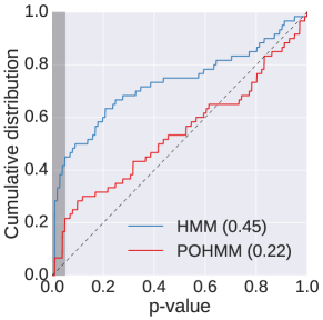
(a) Constrained-text

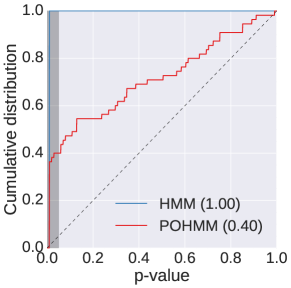
(b) Free-text

Figure 5: Keystroke goodness of fit p-value distributions testing the null hypothesis that the model is consistent with the data. Proportions of rejected samples at the 0.05 significance level are shown in parentheses. If the null hypothesis was true, i.e., the model was actually consistent with the keystroke data, then p-values would follow a uniform distribution shown by the dashed black line.

The test is performed for both the HMM and the POHMM for each user in the fable and essay datasets, using the key-press time intervals only. The resulting p-value distributions are shown in Figure 5. The shaded area represents a 0.05 significance level in which the null hypothesis is rejected. In the fable dataset, the HMM is rejected for 45% of users, while the POHMM is rejected for 22% of users. The HMM is rejected for 100% of users in the essay dataset, and the POHMM is rejected for 40% of users. If the POHMM truly reflected typing behavior (i.e., the null hypothesis was actually true), the p-values would follow a uniform distribution shown by the dashed black line. In both experiments, the POHMM is largely preferred over the HMM.

5.2 Identification and verification

We use the POHMM to perform both user identification and verification, and compare the results to other leading methods. Identification, a multiclass classification problem, is performed by the MAP approach in which the model with maximum a posterior probability is chosen as the class label. This approach is typical in using a generative model to perform classification. Better performance could, perhaps, be achieved through parameter estimation with a discriminative criterion [36], or a hybrid discriminative/generative model in which the POHMM parameters provide features for a discriminative classifier [37]. Verification, a binary classification problem, is achieved by comparing the claimed user’s model loglikelihood to a threshold.

Identification and verification results are obtained for each keystroke dataset and four benchmark anomaly detectors in addition to the POHMM. The password dataset uses a validation procedure similar to Killourhy and Maxion [29], except only samples from the 4th session (repetitions 150-200) are used for training and sessions 5-8 (repetitions 201-400) for testing. For the other datasets, results are obtained through a stratified cross-fold validation procedure with the number of folds equal to the number of samples per user: 20 for keypad and mobile, 4 for fable, and 6 for essay. In each fold, one sample from each user is retained as a query and the remaining samples are used for training.

Identification accuracy (ACC) is measured by the proportion of correctly classified query samples. Verification performance is measured by the user-dependent equal error rate (EER), the point on the receiver operating characteristic (ROC) curve at which the false rejection rate (FRR) and false acceptance rate (FAR) are equal. Each query sample is compared against every model in the population, only one of which will be genuine. The resulting loglikelihood is normalized using the minimum and maximum loglikelihoods from every model in the population to obtain a normalized score between 0 and 1. Confidence intervals for both the ACC and EER are obtained over users in each dataset, similar to [29].

Table 2: Identification accuracy rates. Bold indicates systems that are not significantly worse than the best system. Mobile+ includes mobile sensor features in addition to time intervals.

	Manhattan	Manhattan (Scaled)	SVM (One-class)	HMM	POHMM
Password	0.510 (0.307)	0.662 (0.282)	0.465 (0.293)	0.467 (0.295)	0.789 (0.209)
Keypad	0.623 (0.256)	0.713 (0.200)	0.500 (0.293)	0.478 (0.287)	0.748 (0.151)
Mobile	0.290 (0.230)	0.528 (0.237)	0.267 (0.229)	0.303 (0.265)	0.607 (0.189)
Mobile+	0.647 (0.250)	0.947 (0.104)	0.857 (0.232)	0.937 (0.085)	0.971 (0.039)
Fable	0.492 (0.332)	0.613 (0.314)	0.571 (0.235)	0.392 (0.355)	0.887 (0.175)
Essay	0.730 (0.320)	0.839 (0.242)	0.342 (0.302)	0.303 (0.351)	0.909 (0.128)

Benchmark anomaly detectors include Manhattan distance, scaled Manhattan distance, one-class support vector machine (SVM), and a two-state HMM. The Manhattan, scaled Manhattan, and one-class SVM operate on fixed-length feature vectors, unlike the HMM and POHMM. Timing feature vectors for the password, keypad, and mobile datasets are formed by the 11 press-press latencies and 10 durations of each 11-keystroke sample for a total of 21 timing features. The mobile sensors provide an additional 10 features for each keystroke event for a total of 131 features. For each event, the sensor features include: acceleration (meters/second²) and rotation (radians/second) along three orthogonal axes (6 features), screen coordinates (2 features), pressure (1 feature), and the length of the major axis of an ellipse fit to the pointing device (1 feature). Feature vectors for the fable and essay datasets are each comprised of a set of 218 descriptive statistics for various keystroke timings. Such timing features include the sample mean and standard deviation of various sets of key durations, e.g., consonants, and latency between sets of keys, e.g., from consonants to vowels. For a complete list of features see [33, 38]. The feature extraction also includes a rigorous outlier removal step that excludes observations outside a specified confidence interval and a hierarchical fallback scheme that accounts for missing or infrequent observations.

The Manhattan anomaly detector uses the negative Manhattan distance to the mean template vector as a confidence score. For the scaled Manhattan detector, features are first scaled by the mean absolute deviation over the entire dataset. This differs slightly from the scaled Manhattan in [29], which uses the mean absolute deviation of each user template. The global (over the entire dataset) mean absolute deviation is used in this work due to the low number of samples per user in some datasets. The one-class SVM uses a radial basis function (RBF) kernel and 0.5 tolerance of training errors, i.e., half the samples will become support vectors. The HMM is exactly the same as the POHMM (two hidden states and log-normal emissions), except event types are ignored.

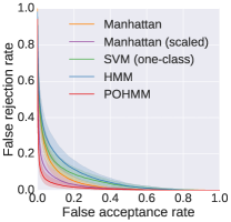
(a) Password

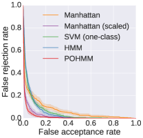
(b) Keypad

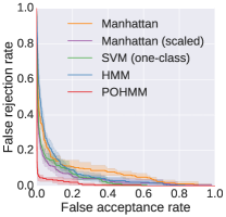
(c) Fixed-text

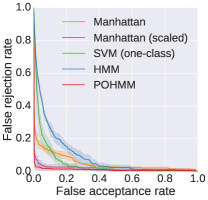
(d) Free-text

Figure 6: Keystroke ROC curves. Bands show the 95% confidence intervals.

Table 3: User-dependent EER. Bold indicates systems that are not significantly worse than the best system. Mobile+ includes mobile sensor features in addition to time intervals.

	Manhattan	Manhattan (scaled)	SVM (one-class)	HMM	POHMM
Password	0.088 (0.069)	0.062 (0.064)	0.112 (0.088)	0.126 (0.099)	0.042 (0.051)
Keypad	0.092 (0.069)	0.053 (0.030)	0.110 (0.054)	0.099 (0.050)	0.053 (0.025)
Mobile	0.194 (0.101)	0.097 (0.057)	0.170 (0.092)	0.168 (0.085)	0.090 (0.054)
Mobile+	0.084 (0.061)	0.009 (0.027)	0.014 (0.033)	0.013 (0.021)	0.006 (0.014)
Fable	0.085 (0.091)	0.049 (0.060)	0.099 (0.106)	0.105 (0.092)	0.031 (0.077)
Essay	0.061 (0.092)	0.028 (0.052)	0.098 (0.091)	0.145 (0.107)	0.020 (0.046)

Identification and verification results are shown in Tables 2 and 3, respectively, and ROC curves are shown in Figure 6. The best-performing anomaly detectors in Tables 2 and 3 are shown in bold. The set of best-performing detectors contains those that are not significantly worse than the POHMM, which achieves the highest performance in every experiment. The Wilcoxon signed-rank test is used to determine whether a detector is significantly worse than the best detector, testing the null hypothesis that a detector has the same performance as the POHMM. A Bonferroni correction is applied to control the family-wise error rate, i.e., the probability of falsely rejecting a detector that is actually in the set of best-performing detectors [39]. At a 0.05 significance level, the null hypothesis is rejected with a p-value not greater than $\frac{0.05}{4}$ since four tests are applied in each row. The POHMM achieves the highest identification accuracy and lowest equal error rate for each dataset. For 3 out of 6 datasets in both sets of experiments, all other detectors are found to be significantly worse than the POHMM.

5.3 Continuous verification

Continuous verification has been recognized as a problem in biometrics whereby a resource is continuously monitored to detect the presence of a genuine user or impostor [40]. It is natural to consider the continuous verification of keystroke dynamics, and most behavioral biometrics, since events are continuously generated as the user interacts with the system. In this case, it is desirable to detect an impostor within as few keystrokes as possible. This differs from the static verification scenario in the previous section in which verification performance is evaluated over an entire session. Instead, continuous verification requires a verification decision to be made upon each new keystroke [23].

Continuous verification is enforced through a penalty function in which each new keystroke incurs a non-negative penalty within a sliding window. The penalty at any given time can be thought of as the inverse of trust. As behavior becomes more consistent with the model, the cumulative penalty within the window can decrease, and as it becomes more dissimilar, the penalty increases. The user is rejected if the cumulative penalty within the sliding window exceeds a threshold. The threshold is chosen for each sample such that the genuine user is never rejected, analogous to a 0% FRR in static verification. An alternative to the penalty function is the penalty-and-reward function in which keystrokes incur either a penalty or a reward (i.e., a negative penalty) [41]. In this work, the sliding window replaces the reward since penalties outside the window do not contribute towards the cumulative penalty.

The penalty of each new event is determined as follows. The marginal probability of each new event, given the preceding events, is obtained from the forward lattice, $\alpha$, given by

$$P\left({\bf x}_{n+1}|{\bf x}_{1}^{n}\right)=P\left({\bf x}_{1}^{n+1}\right)-P\left({\bf x}_{1}^{n}\right)$$ (43)

When a new event is observed, the likelihood is obtained under every model in a population of $U$ models. The likelihoods are ranked, with the highest model given a rank of 0, and the lowest a rank of $U-1$. The rank of the claimed user’s model is the incurred penalty. Thus, if a single event is correctly matched to the genuine user’s model, a penalty of 0 is incurred; if it scores the second highest likelihood, a penalty of 1 is incurred, etc. The rank penalty is added to the cumulative penalty in the sliding window, while penalties outside the window are discarded. A window of length 25 is used in this work.

Continuous verification performance is reported as the number of events (up to the sample length) that can occur before an impostor is detected. This is determined by increasing the penalty threshold until the genuine user is never rejected by the system. Since the genuine user’s penalty is always below the threshold, this is the maximum number of events that an impostor can execute before being rejected by the system while the genuine user is never rejected.

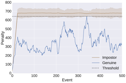
Figure 7: Continuous verification example. Bands show the 95% confidence interval. In this example, impostors are detected after an average of 81 keystrokes.

An example of the penalty function for genuine and impostor users is shown in Figure 7. The decision threshold is set to the maximum penalty incurred by the genuine user so that a false rejection does not occur. The average penalty for impostor users with 95% confidence interval is shown. In this example, the impostor penalties exceed the decision threshold after 81 keystrokes on average. Note that this is different than the average imposter penalty, which exceeds the threshold after 23 keystrokes.

For each dataset, the average maximum rejection time (AMRT) is determined, shown in Table 4. The maximum rejection time (MRT) is the maximum number of keystrokes needed to detect an impostor without rejecting the genuine user, or the time to correct reject (TCR) with perfect usability [40]. The MRT is determined for each combination of impostor query sample and user model in the dataset to get the AMRT. The POHMM has a lower AMRT than the HMM for every dataset, and less than half that of the HMM for free-text input.

Table 4: Continuous verification average maximum rejection time: the number of events that occur before an impostor is detected given the genuine user is not falsely rejected.

	HMM	POHMM
Password	5.64 (2.04)	3.42 (2.04)
Keypad	4.54 (2.09)	3.45 (1.73)
Mobile	5.63 (2.18)	4.29 (2.02)
Mobile+	0.15 (0.65)	0.12 (0.57)
Fable	33.63 (15.47)	20.81 (9.07)
Essay	129.36 (95.45)	55.18 (68.31)

6 Discussion

There have been several generalizations of the standard HMM to deal with hidden states that are partially observable in some way. These models are referred to as partly-HMM [42], partially-HMM [43], and context-HMM [44].

The partly-HMM is a second order model in which the first state is hidden and the second state is observable [42]. In the partly-HMM, both the hidden state and emission at time $t_{n}$ depend on the observation at time $t_{n-1}$. The partly-HMM can be applied to problems that have a transient underlying process, such as gesture and speech recognition, as opposed to a piecewise stationary process that the HMM assumes [45]. Parameter estimation is performed by the EM algorithm, similar to the HMM.

Partially observable states can also come in the form of partial and uncertain ground truth regarding the hidden state at each time step. The partially-HMM addresses this scenario, in which an uncertain hidden state label may be observed at each time step [43]. The probability of observing the uncertain label and the probability of the label being correct, were the true hidden state known, are controlled by parameters $p_{obs}$ and $p_{true}$, respectively. Thus, the probability of observing a correct label is $p_{obs}\times p_{true}$. This model is motivated by language modeling applications in which manually labeling data is expensive and time consuming. Similar to the HMM, the EM algorithm can be used for estimating the parameters of the partially-HMM [43].

Past observations can also provide context for the emission and hidden state transition probabilities in an HMM. Forchhammer and Rissanen [44] proposed the context-HMM, in which the emission and hidden state probabilities at time $t_{n+1}$ are conditioned on contexts $r_{n}$ and $s_{n}$, respectively. Each context is given by a function of the previous observations up to time $t_{n}$. The context-HMM has information theoretic motivations, with applications such as image compression [46]. Used in this way, the neighboring pixels in an image can provide context for the emission and transition probabilities.

There are two scenarios in which previous models of partial observability fall short. The first is when there is missing data during parameter estimation, such missing context, and the second is when there is missing or novel data during likelihood calculation. A possible solution to these problems uses the explicit marginal emission and transition distributions, where, e.g., the context is marginalized out. While none of the above models possess this property, the POHMM, described in Section 3, has explicit marginal distributions that are used when missing or novel data are encountered. Additionally, parameter smoothing uses the marginal distributions to regularize the model and improve parameter estimates.

The POHMM is different from the partly-HMM [42], being a first order model, and different from the partially-HMM [43], since it doesn’t assume a partial labeling. The POHMM is most similar to the context-HMM [44] in the sense that emission and transition probabilities are conditioned on some observed values. Despite this, there are several important differences between the POHMM and context-HMM:

1. The context is not a function of the previous emissions; instead it is a separate observed value (called an event type in this work).

2. The context for hidden state and emission is the same, i.e., $s_{n}=r_{n}$.

3. The emission at time $n+1$ is conditioned on a context observed at time $n+1$ instead of time $n$.

4. An additional context $s_{n+1}$ is available at time $n+1$, upon which the hidden state is also conditioned.

The first difference enables the POHMM to characterize system behavior that depends on an independent Markov chain which emanates from a completely separate process. Such a scenario is encountered in keystroke dynamics, whereby typing behavior depends on the text that is being typed, but the text itself is not considered part of the keystroke dynamics. This distinction is not made in the context-HMM, as the context is based on the previously-observed emissions. Additionally, the context-HMM, as original described, contains only discrete distributions and lacks explicit marginal distributions; therefore it is unable to account for missing or novel data during likelihood calculation, as would be needed in free-text keystroke dynamics.

7 Conclusions

This work introduced the POHMM, an extension of the HMM in which the hidden states are partially observable through an independent Markov chain. Computational complexities of POHMM parameter estimation and likelihood calculation are comparable to that of the HMM, which are linear in the number of observations. POHMM parameter estimation also inherits the desirable properties of expectation maximization, as a modified Baum-Welch algorithm is employed. A case study of the POHMM applied to keystroke dynamics demonstrates superiority over leading alternative models on a variety of tasks, including identification, verification, and continuous verification.

Since we assumed the event type is given, we considered only the conditional likelihood $P\left({\bf x}_{1}^{N}|\Omega_{1}^{N}\right)$. Consideration of the joint likelihood $P\left({\bf x}_{1}^{N},\Omega_{1}^{N}\right)$ remains an item for future work. Applied to keystroke dynamics, the joint likelihood $P\left({\bf x}_{1}^{N},\Omega_{1}^{N}\right)$ would reflect both the keystroke timings and keys typed enabling the model to capture both typing behavior and text generation. Alternatively, the consideration of $P\left(\Omega_{1}^{N}|{\bf x}_{1}^{N}\right)$ would enable the POHMM to recover the key names from keystroke timings, also an item for future work.

Appendix A Summary of POHMM parameters and variables

Table 5: Summary of POHMM parameters and variables.

Parameter	Description
$\psi$,$\omega$	Event types
$i$, $j$	Hidden states
${\bf x}_{1}^{N}$	Observation sequence; ${\bf x}_{n}$ is the feature vector observed at time $t_{n}$
$\Omega_{1}^{N}$	Event type sequence; $\Omega_{n}$ is the event type observed at time $t_{n}$
$z_{1}^{N}$	Sequence of hidden (unobserved) states; $z_{n}$ is the hidden state at time $t_{n}$
$M$	Number of hidden states
$m$	Number of unique event types in $\Omega_{1}^{N}$
$a\left[i,j|\psi,\omega\right]$	Probability of transitioning from state $i$ to $j$, given event types $\psi$ while in state $i$ and $\omega$ in state $j$
$\pi\left[j|\omega\right]$	Probability of state $j$ at time $t_{1}$, given event type $\omega$
$\Pi\left[j|\omega\right]$	Stationary probability of state $j$, given event type $\omega$
${\bf b}\left[j|\omega\right]$	Emission distribution parameters of state $j$, given event type $\omega$
$\gamma_{n}\left[j|\omega\right]$	Probability of state $j$ at time $t_{n}$, given event type $\omega$
$\xi_{n}\left[i,j|\psi,\omega\right]$	Probability of transitioning from state $i$ at time $t_{n}$ to state $j$ at time $t_{n+1}$, given event types $\psi$ and $\omega$ at times $t_{n}$ and $t_{n+1}$, respectively

Appendix B Proof of convergence

The proof of convergence follows that of Levinson et al. [47] which is based on Baum et al. [48]. Only the parts relevant to the POHMM are described. Let $Q\left(\theta,\dot{\theta}\right)$ be Baum’s auxiliary function,

$$Q\left(\theta,\dot{\theta}\right)=\sum_{z_{1}^{N}\in Z}\ln u_{z_{1}^{N}}\ln v_{z_{1}^{N}}$$ (44)

where $u_{z_{1}^{N}}=P\left({\bf x}_{1}^{N},z_{1}^{N}|\Omega_{1}^{N},\theta\right)$, $v_{Z}=P\left({\bf x}_{1}^{N},z_{1}^{N}|\Omega_{1}^{N},\dot{\theta}\right)$, and $Z$ is the set of all state sequences of length $N$. By Theorem 2.1 in Baum’s proof [48], maximizing $Q\left(\theta,\dot{\theta}\right)$ leads to increased likelihood, unless at a critical point, in which case there is no change.

Using the POHMM parameters $\dot{\theta}$, $\ln v_{z_{1}^{N}}$ can be written as

$$\ln v_{z_{1}^{N}} = \ln P\left(z_{1}^{N},{\bf x}_{1}^{N}|\Omega_{1}^{N},\dot{\theta}\right)$$ (46)

$$= \ln\dot{\pi}\left[z_{1}|\Omega_{1}\right]+\sum_{n=1}^{N-1}\ln\dot{a}\left[z_{n},z_{n+1}|\Omega_{n},\Omega_{n+1}\right]+$$

$$\sum_{n=1}^{N}\ln f\left({\bf x}_{n};\dot{{\bf b}}\left[z_{n}|\Omega_{n}\right]\right)$$

and similarly for $\ln u_{z_{1}^{N}}$. Then,

$$Q\left(\theta,\dot{\theta}\right) = \sum_{z_{1}^{N}\in Z}\bigg{\{}\ln\dot{\pi}\left[z_{1}|\Omega_{1}\right]+\sum_{n=1}^{N-1}\ln\dot{a}\left[z_{n},z_{n+1}|\Omega_{n},\Omega_{n+1}\right]$$ (47)

$$+\sum_{n=1}^{N}\ln f\left({\bf x}_{n};\dot{{\bf b}}\left[z_{n}|\Omega_{n}\right]\right)\bigg{\}}P\left(z_{1}^{N}|{\bf x}_{1}^{N},\Omega_{1}^{N},\theta\right)$$

and regrouping terms,

$$Q\left(\theta,\dot{\theta}\right) = \sum_{z_{1}\in Z}\ln\dot{\pi}\left[z_{1}|\Omega_{1}\right]P\left(z_{1}|{\bf x}_{1}^{N},\Omega_{1}^{N},\theta\right)$$ (48)

$$+\sum_{z_{n}^{n+1}\in Z}\sum_{n=1}^{N-1}\ln\dot{a}\left[z_{n},z_{n+1}|\Omega_{n},\Omega_{n+1}\right]P\left(z_{n}^{n+1}|{\bf x}_{1}^{N},\Omega_{1}^{N},\theta\right)$$

$$+\sum_{z_{n}\in Z}\sum_{n=1}^{N}\ln f\left({\bf x}_{n};\dot{{\bf b}}\left[z_{n}|\Omega_{n}\right]\right)P\left(z_{n}|{\bf x}_{1}^{N},\Omega_{1}^{N},\theta\right)\;.$$

Finally, substituting in the model parameters and variables gives,

$$Q\left(\theta,\dot{\theta}\right) = \sum_{j=1}^{M}\gamma_{1}\left[j|\Omega_{1}\right]\ln\dot{\pi}\left[j|\Omega_{1}\right]$$ (49)

$$+\sum_{j=1}^{M}\sum_{i=1}^{M}\sum_{n=1}^{N-1}\xi_{n}\left[i,j|\Omega_{n},\Omega_{n+1}\right]\ln\dot{a}\left[i,j|\Omega_{n}|\Omega_{n+1}\right]$$

$$+\sum_{j=1}^{M}\sum_{n=1}^{N}\gamma_{n}\left[j|\Omega_{n}\right]\ln f\left({\bf x}_{n};\dot{{\bf b}}\left[z_{n}|\Omega_{n}\right]\right)$$

The POHMM re-estimation formulae (Equations 12, 14, 15) follow directly from the optimization of each term in Equation 49. Even when parameter smoothing is used, convergence is still guaranteed. This is due to the diminishing effect of the marginal for each parameter, $\lim_{N\to\infty}\tilde{\theta}=\theta$, where $\tilde{\theta}$ are the smoothed parameters.

References

- Baum and Petrie [1966] L. E. Baum, T. Petrie, Statistical inference for probabilistic functions of finite state Markov chains, The annals of mathematical statistics 37 (6) (1966) 1554–1563.
- Rabiner [1989] L. Rabiner, A tutorial on hidden Markov models and selected applications in speech recognition, Proceedings of the IEEE 77 (2) (1989) 257–286.
- Yamato et al. [1992] J. Yamato, J. Ohya, K. Ishii, Recognizing human action in time-sequential images using hidden markov model, in: Proc. IEEE Computer Society Conference on Computer Vision and Pattern Recognition (CVPR), IEEE, 379–385, 1992.
- Hu et al. [1996] J. Hu, M. K. Brown, W. Turin, HMM based online handwriting recognition, IEEE Transactions on pattern analysis and machine intelligence 18 (10) (1996) 1039–1045.
- Espana-Boquera et al. [2011] S. Espana-Boquera, M. J. Castro-Bleda, J. Gorbe-Moya, F. Zamora-Martinez, Improving offline handwritten text recognition with hybrid HMM/ANN models, IEEE transactions on pattern analysis and machine intelligence 33 (4) (2011) 767–779.
- Hinton et al. [2012] G. Hinton, L. Deng, D. Yu, G. E. Dahl, A.-r. Mohamed, N. Jaitly, A. Senior, V. Vanhoucke, P. Nguyen, T. N. Sainath, et al., Deep neural networks for acoustic modeling in speech recognition: The shared views of four research groups, IEEE Signal Processing Magazine 29 (6) (2012) 82–97.
- Wu et al. [2016] D. Wu, L. Pigou, P.-J. Kindermans, N. D.-H. Le, L. Shao, J. Dambre, J.-M. Odobez, Deep dynamic neural networks for multimodal gesture segmentation and recognition, IEEE transactions on pattern analysis and machine intelligence 38 (8) (2016) 1583–1597.
- Yu [2010] S.-Z. Yu, Hidden semi-Markov models, Artificial Intelligence 174 (2) (2010) 215–243.
- Li [2005] Y. Li, Hidden Markov models with states depending on observations, Pattern Recognition Letters 26 (7) (2005) 977 – 984, ISSN 0167-8655.
- Bianne-Bernard et al. [2011] A.-L. Bianne-Bernard, F. Menasri, R. A.-H. Mohamad, C. Mokbel, C. Kermorvant, L. Likforman-Sulem, Dynamic and contextual information in HMM modeling for handwritten word recognition, IEEE transactions on pattern analysis and machine intelligence 33 (10) (2011) 2066–2080.
- Salthouse [1986] T. A. Salthouse, Perceptual, cognitive, and motoric aspects of transcription typing., Psychological bulletin 99 (3) (1986) 303.
- Lee and Hon [1989] K.-F. Lee, H.-W. Hon, Speaker-independent phone recognition using hidden Markov models, IEEE Transactions on Acoustics, Speech, and Signal Processing 37 (11) (1989) 1641–1648.
- Chung and Liu [2008] P.-C. Chung, C.-D. Liu, A daily behavior enabled hidden Markov model for human behavior understanding, Pattern Recognition 41 (5) (2008) 1572 – 1580, ISSN 0031-3203.
- Samanta et al. [2014] O. Samanta, U. Bhattacharya, S. Parui, Smoothing of HMM parameters for efficient recognition of online handwriting, Pattern Recognition 47 (11) (2014) 3614 – 3629, ISSN 0031-3203.
- Jurafsky et al. [2000] D. Jurafsky, J. H. Martin, A. Kehler, K. Vander Linden, N. Ward, Speech and language processing: An introduction to natural language processing, computational linguistics, and speech recognition, vol. 2, MIT Press, 2000.
- Laskaris et al. [2009] N. A. Laskaris, S. P. Zafeiriou, L. Garefa, Use of random time-intervals (RTIs) generation for biometric verification, Pattern Recognition 42 (11) (2009) 2787–2796.
- Banerjee and Woodard [2012] S. P. Banerjee, D. L. Woodard, Biometric authentication and identification using keystroke dynamics: A survey, Journal of Pattern Recognition Research 7 (1) (2012) 116–139.
- Monaco and Tappert [2016] J. V. Monaco, C. C. Tappert, Obfuscating Keystroke Time Intervals to Avoid Identification and Impersonation, arXiv preprint arXiv:1609.07612 .
- Wang et al. [2015] H. Wang, T. Tsung-Te Lai, R. R. Choudhury, MoLe: Motion Leaks through Smartwatch Sensors, in: Proc. 21st Annual International Conference on Mobile Computing and Networking (MobiCom), ACM, 2015.
- Asonov and Agrawal [2004] D. Asonov, R. Agrawal, Keyboard acoustic emanations, in: Proc. IEEE Symposium on Security and Privacy (SP), IEEE, 3–11, 2004.
- Song et al. [2001] D. X. Song, D. Wagner, X. Tian, Timing Analysis of Keystrokes and Timing Attacks on SSH., in: Proc. USENIX Security Symposium, vol. 2001, 2001.
- Ali et al. [2015] K. Ali, A. X. Liu, W. Wang, M. Shahzad, Keystroke recognition using wifi signals, in: Proc. 21st Annual International Conference on Mobile Computing and Networking (MobiCom), ACM, 90–102, 2015.
- Bours and Mondal [2015] P. Bours, S. Mondal, Performance evaluation of continuous authentication systems, IET Biometrics 4 (4) (2015) 220–226.
- Idrus et al. [2014] S. Z. S. Idrus, E. Cherrier, C. Rosenberger, P. Bours, Soft biometrics for keystroke dynamics: Profiling individuals while typing passwords, Computers & Security 45 (2014) 147–155.
- Brizan et al. [2015] D. G. Brizan, A. Goodkind, P. Koch, K. Balagani, V. V. Phoha, A. Rosenberg, Utilizing linguistically-enhanced keystroke dynamics to predict typist cognition and demographics, International Journal of Human-Computer Studies .
- Montalvão et al. [2015] J. Montalvão, E. O. Freire, M. A. B. Jr., R. Garcia, Contributions to empirical analysis of keystroke dynamics in passwords, Pattern Recognition Letters 52 (Supplement C) (2015) 80 – 86, ISSN 0167-8655.
- Filho and Freire [2006] J. R. M. Filho, E. O. Freire, On the equalization of keystroke timing histograms, Pattern Recognition Letters 27 (13) (2006) 1440 – 1446, ISSN 0167-8655.
- Maas et al. [2014] A. Maas, C. Heather, C. T. Do, R. Brandman, D. Koller, A. Ng, Offering Verified Credentials in Massive Open Online Courses: MOOCs and technology to advance learning and learning research (Ubiquity symposium), Ubiquity 2014 (May) (2014) 2.
- Killourhy and Maxion [2009] K. S. Killourhy, R. A. Maxion, Comparing anomaly-detection algorithms for keystroke dynamics, in: Proc. IEEE/IFIP International Conference on Dependable Systems & Networks (DSN), IEEE, 125–134, 2009.
- Bakelman et al. [2013] N. Bakelman, J. V. Monaco, S.-H. Cha, C. C. Tappert, Keystroke Biometric Studies on Password and Numeric Keypad Input, in: Proc. European Intelligence and Security Informatics Conference (EISIC), IEEE, 204–207, 2013.
- Coakley et al. [2016] M. J. Coakley, J. V. Monaco, C. C. Tappert, Keystroke Biometric Studies with Short Numeric Input on Smartphones, in: Proc. IEEE 8th International Conference on Biometrics Theory, Applications and Systems (BTAS), IEEE, 2016.
- Killourhy and Maxion [2008] K. Killourhy, R. Maxion, The effect of clock resolution on keystroke dynamics, in: Proc. International Workshop on Recent Advances in Intrusion Detection (RAID), Springer, 331–350, 2008.
- Monaco et al. [2013] J. V. Monaco, N. Bakelman, S.-H. Cha, C. C. Tappert, Recent Advances in the Development of a Long-Text-Input Keystroke Biometric Authentication System for Arbitrary Text Input, in: Proc. European Intelligence and Security Informatics Conference (EISIC), IEEE, 60–66, 2013.
- Villani et al. [2006] M. Villani, C. Tappert, G. Ngo, J. Simone, H. S. Fort, S.-H. Cha, Keystroke biometric recognition studies on long-text input under ideal and application-oriented conditions, in: Proc. Conference on Computer Vision and Pattern Recognition Workshop (CVPRW), IEEE, 39–39, 2006.
- Malmgren et al. [2008] R. D. Malmgren, D. B. Stouffer, A. E. Motter, L. A. Amaral, A Poissonian explanation for heavy tails in e-mail communication, Proceedings of the National Academy of Sciences 105 (47) (2008) 18153–18158.
- Mutsam and Pernkopf [2016] N. Mutsam, F. Pernkopf, Maximum margin hidden Markov models for sequence classification, Pattern Recognition Letters 77 (Supplement C) (2016) 14 – 20, ISSN 0167-8655.
- Bicego et al. [2009] M. Bicego, E. Pe,kalska, D. M. Tax, R. P. Duin, Component-based discriminative classification for hidden Markov models, Pattern Recognition 42 (11) (2009) 2637 – 2648, ISSN 0031-3203.
- Tappert et al. [2009] C. C. Tappert, M. Villani, S.-H. Cha, Keystroke biometric identification and authentication on long-text input, Behavioral biometrics for human identification: Intelligent applications (2009) 342–367.
- Rupert Jr et al. [2012] G. Rupert Jr, et al., Simultaneous statistical inference, Springer Science & Business Media, 2012.
- Sim et al. [2007] T. Sim, S. Zhang, R. Janakiraman, S. Kumar, Continuous verification using multimodal biometrics, IEEE transactions on pattern analysis and machine intelligence 29 (4) (2007) 687–700.
- Bours [2012] P. Bours, Continuous keystroke dynamics: A different perspective towards biometric evaluation, Information Security Technical Report 17 (1) (2012) 36–43.
- Kobayashi and Haruyama [1997] T. Kobayashi, S. Haruyama, Partly-hidden Markov model and its application to gesture recognition, in: Proc. IEEE International Conference on Acoustics, Speech, and Signal Processing (ICASSP), vol. 4, IEEE, 3081–3084, 1997.
- Ozkan et al. [2014] H. Ozkan, A. Akman, S. S. Kozat, A novel and robust parameter training approach for HMMs under noisy and partial access to states, Signal Processing 94 (2014) 490–497.
- Forchhammer and Rissanen [1996] S. O. Forchhammer, J. Rissanen, Partially hidden Markov models, IEEE Transactions on Information Theory 42 (4) (1996) 1253–1256.
- Iobayashi et al. [1999] T. Iobayashi, J. Furuyama, K. Mas, Partly hidden Markov model and its application to speech recognition, in: Proc. IEEE International Conference on Acoustics, Speech, and Signal Processing (ICASSP), vol. 1, IEEE, 121–124, 1999.
- Forchhammer and Rasmussen [1999] S. Forchhammer, T. S. Rasmussen, Adaptive partially hidden Markov models with application to bilevel image coding, Image Processing, IEEE Transactions on 8 (11) (1999) 1516–1526.
- Levinson et al. [1983] S. E. Levinson, L. R. Rabiner, M. M. Sondhi, An introduction to the application of the theory of probabilistic functions of a Markov process to automatic speech recognition, The Bell System Technical Journal 62 (4) (1983) 1035–1074.
- Baum et al. [1970] L. E. Baum, T. Petrie, G. Soules, N. Weiss, A maximization technique occurring in the statistical analysis of probabilistic functions of Markov chains, The annals of mathematical statistics 41 (1) (1970) 164–171.