Frequentist Model Comparison Tests of Sinusoidal Variations in Measurements of Newton’s Gravitational Constant

Abstract

In 2015, Anderson et al Anderson15a have claimed to find evidence for periodic sinusoidal variations (period=5.9 years) in measurements of Newton’s gravitational constant. These claims have been disputed by Pitkin Pitkin15 . Using Bayesian model comparison, he argues that a model with an unknown Gaussian noise component is favored over any periodic variations by more than $e^{30}$. We re-examine the claims of Anderson et al Anderson15a using frequentist model comparison tests, both with and without errors in the measurement times. Our findings lend support to Pitkin’s claim that a constant term along with an unknown systematic offset provides a better fit to the measurements of Newton’s constant, compared to any sinusoidal variations.

1 Introduction

In 2015, Anderson et al Anderson15a have found evidence for periodicities in the measured values of Newton’s gravitational constant ($G$) (using data compiled in  Schlamminger ) with a period of 5.9 years. They also noted that similar variations have been seen in the length of a day Holme , and hence there is a possible correlation between the two. However, these results have been disputed by Pitkin Pitkin15 (hereafter P15). In P15, he examined four different models for the observed values of $G$ and showed using Bayesian model comparison tests that the logarithm of the Bayes factor for a model with constant offset and Gaussian noise compared to sinusoidal variations in $G$ is about 30 (See Table 1 of P15). The analysis was done by considering both a uniform prior and a Jeffreys prior for the parameters. Therefore, from his analysis the data is better fit by a constant offset and an unknown Gaussian noise component. Thereafter, Anderson et al responded to this in a short note Anderson15b , pointing out that they were unable to replicate the claims in P15 using minimization of L1 norm, and they stand by their original claims of sinusoidal variations in $G$. Another difference between the analysis done by P15 and by Anderson et al is that P15 marginalized over the errors in measurement times of $G$, whereas these errors in measurement times ignored by Anderson et al. A periodicity search was also done by Schlamminger et al Schlamminger , which involved minimization of both the L1 and L2 norms. They also argue that a sinusoidal variation with a period of 5.9 years provides a better fit than a straight line. However, the chi-square probabilities for all their models are very small (See Table III of  Schlamminger ).

To resolve this imbroglio, we re-analyze the same data using Maximum Likelihood analysis (both with and without errors in the measured values of $G$) and do frequentist model comparison tests between different models. Therefore, our analysis is complementary to that of Anderson Anderson15a and Schlamminger Schlamminger .

2 Analysis summary

The sinusoidal model to which we fit the measurements of $G$ (obtained using a set of measurements $y_{i}$) at times $t_{i}$ is given by Anderson15a :

$$y_{i}=A\sin[\phi_{0}+2\pi(t_{i}/P)]+\mu_{G},$$ (1)

where $\mu_{G}$ is a constant offset, $P$ is the period of the sinusoid, $A$ is the amplitude of the modulation, and $\phi_{0}$ its phase.

Similar to P15, we examine four different model hypotheses and use the same notation:

1. H1 : Data is consistent with Gaussian errors, given by the measured uncertainties $\sigma_{i}$ ;

2. H2 : Same as H1, but data contains an additional unknown offset ($\sigma_{sys}$) ;

3. H3 : Data is described by Eq 1;

4. H4 : Same as H3, with an additional systematic offset in the data.

For each of the above hypothesis, we perform a maximum likelihood-based parameter estimation. Our maximum likelihood (valid when the dependent variables contain no errors) can be written as astroml :

$${\cal L}=\prod_{i=1}^{n}\frac{1}{\sigma_{i}\sqrt{2\pi}}\exp\left\{-\frac{y_{i}-f(t,\mu,P,\phi_{0})}{\sqrt{2}\sigma_{i}}\right\}^{2},$$ (2)

where $f(t,\mu,P,\phi_{0})$ is given by Eq. 1 for H3 and H4, else is equal to a constant offset. For H1 and H3, $\sigma_{i}$ denotes the measured errors in $G$, whereas for H2 and H4, $\sigma_{i}$ is the quadrature sum of the measured uncertainties in $G$ and an unknown systematic term $\sigma_{sys}$.

We use the same data for our tests as P15 (a detailed documentation of his analysis can be found on github). In all, this consists of 12 measurements of $G$ from 1981 to 2013. Similar to P15, we have excluded the measurements by Karagioz & Izmailov. References to all the other measurements can be found in Refs. Anderson15a and  Mohr .

2.1 Model Comparison without errors in measurement times

We now describe the results of our analysis without considering the errors in the measurement times. Results after including the errors shall be described in the next sub-section. The first step in model comparison involves finding the best-fit parameters for each of the four hypotheses by maximizing Eq. 2 for the pertinent model. Naively, one might select the best model as the one with the largest value of the likelihood. But in model selection, one also needs to account for the different numbers of free parameters in each model. In Bayesian statistics, this is usually done by comparing the model posteriors, as discussed and implemented in P15. Other techniques involve the use of penalized likelihoods such as Akaike information criterion, Bayesian information criterion, etc Shafer . However, the results of any Bayesian model comparison test depends upon the choice of prior used for the model or the priors for parameters within each model.

Therefore, to complement the Bayesian model comparison tests done in P15, we perform a frequentist model comparison. We assume that for the correct model, the data is normally distributed around the best-fit model with variance $\sigma_{i}^{2}$. Therefore, the sum of squares of the normalized residuals around the best-fit model should follow $\chi^{2}$ distribution for the correct model after including the degrees of freedom for each model astroml ; Press92 . After finding the best-fit model parameters for each hypothesis, we compare the chi-square probability for the total degrees of freedom ($\nu$), given by astroml ; Press92 ,

$$P(\chi^{2},\nu)=\frac{(\chi^{2})^{(0.5\nu-1)}\exp(-0.5\chi^{2})}{2^{0.5\nu}\mathrm{\Gamma}(0.5\nu)},$$ (3)

where for each model $f(x)$,

$$\chi^{2}=\sum\limits_{i=1}^{N}\frac{\left(y_{i}-f(x)\right)^{2}}{\sigma_{i}^{2}}.$$ (4)

The best-fit model is the one with the largest value of $P(\chi^{2},\nu)$. We use the Amoeba Press92 minimization technique and as initial starting guesses for the model parameters in H3 and H4, we used the best-fit values found by Anderson et al. Note that for H3 and H4, in all there are only 12 data points and four (five) free parameters and so we expect a number of false minima for the four (five) dimensional parameter space (See for eg. Schlamminger ). We do not explore these false minima here, as our main goal is to test the claims in Ref. Anderson15a .

Our results for all the four models can be found in Tab. 1. The measurements for $G$ along with the best-fit model parameters for the hypotheses H1, H2, and H3 are shown in Fig. 1. We can see that the best-fit model is hypothesis H2, which consists of a constant offset and unknown systematic noise component. It is a better description of the data compared to sinusoidal variations. Our results were obtained by a complementary model comparison method. We conclude that the measurements of $G$ do not support a sinusoidal variation, without allowing for any errors in the measurement times, in agreement with P15.

Table 1: Summary of model comparison tests without including the errors in measurement for each of the four hypotheses H1, H2, H3, and H4. $A$, $\mu$, $P$, $\sigma_{sys}$ are defined in Eq. 1. For each of the hypotheses, we show $\chi^{2}/DOF$ and P($\chi^{2}$,$\nu$). As we can see, P($\chi^{2}$,$\nu$) is largest for H2 (which is a constant offset and an unknown systematic). Therefore, the measurements do not favor a sinusoidal variation compared to a constant offset and a systematic term.

Hypothesis	$\mu$	$\sigma_{sys}$	$A$	$P(yrs)$	$\phi_{0}$	DOF	$\chi^{2}/DOF$	P($\chi^{2}$,$\nu$)
H1	$6.766\times 10^{-11}$	-	-	-	-	11	28.04	$6.8\times 10^{-60}$
H2	$6.674\times 10^{-11}$	$10^{-14}$	-	-	-	10	1.27	0.059
H3	$6.674\times 10^{-11}$	-	$1.64\times 10^{-14}$	$5.9$	$-0.07$	8	2.93	0.0011
H4	$6.571\times 10^{-11}$	$10^{-12}$	$1.9\times 10^{-14}$	$7.57$	0.0011	7	1.71	0.032

Table 2: Summary of model comparison tests after including errors in measurement times. The results for hypothesis H1 and H2 will be same as in Tab. 1 and are not shown in this table.

Hypothesis	$\mu$	$\sigma_{sys}$	$A$	$P(yrs)$	$\phi_{0}$	DOF	$\chi^{2}/DOF$	P($\chi^{2}$,$\nu$)
H3	$6.674\times 10^{-11}$	-	$1.64\times 10^{-14}$	$5.9$	$-0.07$	8	2.93	0.0011
H4	$6.571\times 10^{-11}$	$10^{-12}$	$1.9\times 10^{-14}$	$7.57$	0.0011	7	1.71	0.033

2.2 Model Comparison after including errors in measurement times

We now redo the analysis by including the uncertainties in measurement times. We use the same values for these as in P15, which is $\sigma_{t}$=0.25 years for all the measurements, except for JILA-10 and LENS-14 for which $\sigma_{t}$= 1 week. To include the uncertainties in the dependent variables, we follow the formalism by Weiner et al Weiner , which has been used in a number of astrophysical analyses from galaxy clusters to pulsars Hoekstra ; Desai15 . Briefly, the likelihood is the same as in Eq. 2. Only $\sigma_{i}$ gets modified and the new uncertainty $\sigma_{net}$ is given by

$$\sigma_{net}=\sqrt{\sigma_{i}^{2}+\left(\frac{\partial y}{\partial t}\right)^{2}\sigma_{t}^{2}}.$$ (5)

Intuitively, we would expect the $\chi^{2}$/DOF to be smaller compared to any fitting done without errors in the dependent variable. The best-fit values, $\chi^{2}/dof$, and P($\chi^{2},\nu$) for H3 and H4 are shown in Tab. 2. As we can see, even after including the errors in the dependent variable, the chi-square probabilities are smaller for H3 and H4 compared to H2. Therefore, the data still supports a constant offset and a systematic uncertainty compared to a sinusoidal variation, even after the inclusion of errors in measurement times.

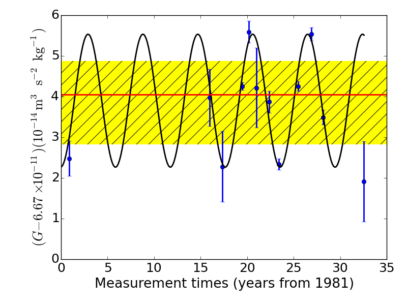
Figure 1: Data showing variation of Newton’s Constant ($G$) as a function of time. The blue points indicate the measurements (same as those used in P15 Pitkin15 , which contains links to original references). The red line shows best-fit constant offset for hypothesis H1. The yellow hatched region indicates best-fit for hypothesis H2. The black sinusoidal curve shows the best-fit parameters for hypothesis H3.

3 Conclusions

The current consensus among the Physics and Astrophysics community is that measurements of Newton’s Gravitational constant ($G$) have no time dependence or any correlations with environmental parameters. However, this paradigm has recently been challenged by Anderson and collaborators Anderson15a . They have detected sinusoidal variations in the measurements of Newton’s constant ($G$) (compiled over the last 35 years from 1981) with a period of 5.9 years Anderson15a ; Anderson15b . Similar periodic variations have also been observed in measurements of the length of the day Holme . Therefore, Anderson et al have argued there is some systematic effect in measurements of $G$ that is connected with the same mechanism, which causes variations in the length of the day. However, these results have been disputed by Pitkin Pitkin15 , who has shown using Bayesian model comparison and a suitable choice of priors for the different model parameters, that a model with constant offset and a unknown systematic uncertainty fits the data better than any sinusoidal variations, with the Bayes factor between the two hypotheses having a value equal to $e^{30}$. Therefore, the analysis by Pitkin contradicts the claims by Anderson et al.

In this letter, we have carried out a complementary analysis of the same dataset to resolve the above conflicting claims between the two groups of authors. We have performed frequentist model comparison tests of the same measurements, both with and without the errors in measurement times. We examined four hypotheses similar to that in Ref. Pitkin15 : a constant offset; a constant offset augmented by an unknown systematic uncertainty; sinusoidal variations; and sinusoidal variations with an unknown systematic uncertainty. For each of these models, we found the best-fit parameters and then calculated the chi-square probabilities for each of these and chose the best model as the one with the largest chi-square probability. This is the standard procedure followed in frequentist model comparison, which is complementary to the Bayesian model comparison analysis done by Pitkin.

We find in agreement with Pitkin that the best model is the one with a constant offset in measurements of $G$ along with an unknown systematic offset. Therefore, there is no evidence for any sinusoidal variations in the measurements of $G$.

- (1) J.D. Anderson, G. Schubert, V. Trimble, M.R. Feldman, EPL (Europhysics Letters) 110, 10002 (2015). DOI 10.1209/0295-5075/110/10002
- (2) M. Pitkin, EPL (Europhysics Letters) 111, 30002 (2015). DOI 10.1209/0295-5075/111/30002
- (3) S. Schlamminger, J.H. Gundlach, R.D. Newman, Phys. Rev. D91(12), 121101 (2015). DOI 10.1103/PhysRevD.91.121101
- (4) R. Holme, O. De Viron, Nature 499(7457), 202 (2013)
- (5) J.D. Anderson, G. Schubert, V. Trimble, M.R. Feldman, EPL (Europhysics Letters) 111, 30003 (2015). DOI 10.1209/0295-5075/111/30003
- (6) J. Vanderplas, A. Connolly, Ž. Ivezić, A. Gray, in Conference on Intelligent Data Understanding (CIDU) (2012), pp. 47 –54. DOI 10.1109/CIDU.2012.6382200
- (7) P.J. Mohr, B.N. Taylor, D.B. Newell, Reviews of Modern Physics 84, 1527 (2012). DOI 10.1103/RevModPhys.84.1527
- (8) D.L. Shafer, Phys. Rev. D91(10), 103516 (2015). DOI 10.1103/PhysRevD.91.103516
- (9) W.H. Press, S.A. Teukolsky, W.T. Vetterling, B.P. Flannery, Numerical recipes in C. The art of scientific computing (1992)
- (10) B.J. Weiner, C.N.A. Willmer, S.M. Faber, J. Harker, S.A. Kassin, A.C. Phillips, J. Melbourne, A.J. Metevier, N.P. Vogt, D.C. Koo, ApJ653, 1049 (2006). DOI 10.1086/508922
- (11) H. Hoekstra, A. Mahdavi, A. Babul, C. Bildfell, Mon. Not. Roy. Ast. Soc.427, 1298 (2012). DOI 10.1111/j.1365-2966.2012.22072.x
- (12) S. Desai, Astrophys. and Space Sci.361, 138 (2016). DOI 10.1007/s10509-016-2726-z