ILC–NOTE–2016–067 DESY 16–145, IPMU16-0108 KEK Preprint 2016–9, LAL 16–185 MPP–2016–174, SLAC–PUB–16751 July, 2016

Implications of the 750 GeV $\gamma\gamma$ Resonance as a Case Study for the International Linear Collider

LCC Physics Working Group

Keisuke Fujii¹, Christophe Grojean^2,3 Michael E. Peskin⁴(conveners); Tim Barklow⁴, Yuanning Gao⁵, Shinya Kanemura⁶, Hyungdo Kim⁷, Jenny List², Mihoko Nojiri^1,8, Maxim Perelstein⁹, Roman Pöschl¹⁰, Jürgen Reuter², Frank Simon¹¹, Tomohiko Tanabe¹², Jaehoon Yu¹³, James D. Wells¹⁴; Adam Falkowski¹⁵, Shigeki Matsumoto⁸,
Takeo Moroi¹⁶, Francois Richard¹⁰, Junping Tian¹², Marcel Vos¹⁷, Hiroshi Yokoya¹⁸; Hitoshi Murayama^8,19,20, Hitoshi Yamamoto²¹

ABSTRACT

If the $\gamma\gamma$ resonance at 750 GeV suggested by 2015 LHC data turns out to be a real effect, what are the implications for the physics case and upgrade path of the International Linear Collider? Whether or not the resonance is confirmed, this question provides an interesting case study testing the robustness of the ILC physics case. In this note, we address this question with two points: (1) Almost all models proposed for the new 750 GeV particle require additional new particles with electroweak couplings. The key elements of the 500 GeV ILC physics program—precision measurements of the Higgs boson, the top quark, and 4-fermion interactions—will powerfully discriminate among these models. This information will be important in conjunction with new LHC data, or alone, if the new particles accompanying the 750 GeV resonance are beyond the mass reach of the LHC. (2) Over a longer term, the energy upgrade of the ILC to 1 TeV already discussed in the ILC TDR will enable experiments in $\gamma\gamma$ and $e^{+}e^{-}$ collisions to directly produce and study the 750 GeV particle from these unique initial states.

 

¹ High Energy Accelerator Research Organization (KEK), Tsukuba, Ibaraki, JAPAN
² DESY, Notkestrasse 85, 22607 Hamburg, GERMANY
³ ICREA at IFAE, Univesitat Autónoma de Barcelona, E-08193 Bellaterra, SPAIN
⁴ SLAC, Stanford University, Menlo Park, CA 94025, USA
⁵ Center for High Energy Physics, Tsinghua University, Beijing, CHINA
⁶ Department of Physics, University of Toyama, Toyama 930-8555, JAPAN
⁷ Department of Physics and Astronomy, Seoul National University, Seoul 151-747,
         KOREA
⁸ Kavli Institute for the Physics and Mathematics of the Universe,
         University of Tokyo, Kashiwa 277-8583, JAPAN
⁹ Laboratory for Elementary Particle Physics, Cornell University, Ithaca, NY 14853,
         USA
¹⁰ LAL, Centre Scientifique d’Orsay, Université Paris-Sud, F-91898 Orsay CEDEX,
         FRANCE
¹¹ Max-Planck-Institut fü̈r Physik, Fö̈hringer Ring 6, 80805 Munich, GERMANY
¹² ICEPP, University of Tokyo, Hongo, Bunkyo-ku, Tokyo, 113-0033, JAPAN
¹³ Department of Physics, University of Texas, Arlington, TX 76019, USA
¹⁴ Michigan Center for Theoretical Physics, University of Michigan, Ann Arbor,
         MI 48109, USA
¹⁵ LPT, Université Paris-Sud, 91405 Orsay, FRANCE
¹⁶ Department of Physics, University of Tokyo, Tokyo 113-0033, JAPAN
¹⁷ IFIC (UVEG/CSIC), Edificios de Investigacion, c./ Catedratico Jose Beltran 2, E-46980 Paterna, Valencia, SPAIN
¹⁸ Quantum Universe Center, KIAS, Seoul 02455, KOREA
¹⁹ Department of Physics, University of California, Berkeley, CA 94720, USA
²⁰ Theoretical Physics Group, Lawrence Berkeley National Laboratory, Berkeley,
         CA 94720, USA
²¹ Department of Physics, Tohoku University, Sendai, Miyagi 980-8578, JAPAN

 

 

1 Introduction

There are many arguments that there exist new interactions of physics beyond the currently defined Standard Model (SM) of particle physics. The main features of the observed universe—the presence of a small, nonzero dark energy, the presence of cold dark matter at a total mass 5 times that of atomic matter, and the prevalence of baryons over antibaryons—cannot be accounted for by the SM. However, today there are no unambiguous signals that point to a strategy for exploring for physics beyond the SM. We fall back, then, on the obvious strategies of searching for new particles at high energy and measuring the properties of known particles with increasing precision.

If we could have more specific information about the nature of the new physics, this might help us define better the goals of a program of future accelerator experiments. It is interesting to look even at suggested anomalies in the data in this light. We should ask: If the suggested effect is confirmed, what path to new physics would be suggested, and how can proposed future accelerator facilities explore this path?

In December 2015, the ATLAS and CMS collaborations presented very preliminary evidence for a resonance at a mass of about 750 GeV, created in $pp$ collisions and decaying to $\gamma\gamma$ [1, 2]. These results, and the results of the searches for $\gamma\gamma$ resonances in the 8 TeV data, were recently updated [3, 4]. At this time, the evidence for this resonance is hardly persuasive. ATLAS quotes a local significance of the effect in the 13 TeV data at about 3.7 $\sigma$ and a global significance of 2.0 $\sigma$, and a local significance in the 8 TeV data of 1.9 $\sigma$. CMS reports a peak with local significance 2.8 $\sigma$ and a small compatible effect in the 8 TeV data. This would be unremarkable except that its location seems to coincide with the peak location found by ATLAS. Clearly, more data is needed to confirm this observation.

The purpose of this note is to gather information on the question: If the resonance suggested by the LHC data is real, what would the implications be for the program of the International Linear Collider? Will the ILC be able to shed light on this resonance or on accompanying new physics? For definiteness, we refer to the resonance from here on as $\Phi$.

Since the ILC is designed for an energy of 500 GeV, it will not be able to produce the $\Phi$ directly. The ILC TDR foresees an upgrade of the accelerator to a center of mass energy of 1000 GeV, and this machine will be able to produce $\Phi$ either from the $e^{+}e^{-}$ or from the $\gamma\gamma$ initial state. One might discuss a $\gamma\gamma$ collider optimized for $\Phi$ production, and we will give parameters below, following [5, 6, 7, 8, 9].

However, a discussion of the implications of the $\Phi$ resonance should not focus exclusively on direct observation of the $\Phi$. As we will discuss, in most of the models that have been proposed for the identity of the $\Phi$, this resonance is one of many new particles that must be introduced. In most models, other required new particles should be discovered at the LHC. It might turn out that the $\Phi$ is a relatively minor player in a new sector of physics that the LHC will begin to uncover in the next few years. For this reason, it is premature to discuss a new accelerator intended specifically to target the $\Phi$ or any other new particle that turns up in the early 13 TeV LHC data.

The relation of the ILC to the $\Phi$, however, is quite different. In presentations of the physics goals of the ILC (for example, [10, 11, 12]), it is always emphasized that the ILC at 500 GeV offers techniques for observing effects of new physics that are orthogonal to those of direct particle search at the LHC and are sensitive to a broad range of new physics models. These include precision measurements of the couplings of the Higgs boson, the electroweak couplings of the top quark, the 3-boson couplings of the $W$ and $Z$ bosons, and interactions mediating fermion-fermion scattering. If the observation of the $\Phi$ is confirmed, and even if the LHC discovers further additional new particles related to the $\Phi$, these techniques will be indispensable to discriminate possible explanations of the resonance and to demonstrate the presence of further states beyond the reach of the LHC. If the $\Phi$ is not confirmed, these techniques will still provide a means to search for physics beyond the Standard Model and might provide the first discovery of new physics.

The models that have been suggested for the identity of the $\Phi$ highlight these capabilities by predicting substantial effects in the ILC precision experiments. As such, they provide a worked example of the impact of the ILC precision measurements. The study of this example gives insight, whether or not the $\Phi$ turns out to be a real signal.

The structure of this note is as follows: In Section 2, we review basic properties of the $\Phi$ resonance necessary for our discussion. In Section 3, the heart of the paper, we present the importance of precision measurements on Higgs, top, and 4-fermion interactions for a variety of specific models that have been proposed for the $\Phi$. At the same time, we should not ignore the capabilities of an energy-upgraded ILC to directly produce the $\Phi$ and its partners. In Section 4, we discuss the observation of the $\Phi$ at the ILC, upgraded to 1000 GeV, in $\gamma\gamma$ and $e^{+}e^{-}$ collisions, and the possibility of a $\gamma\gamma$ collider optimized for the $\Phi$ resonance.

2 Properties of the $\Phi$

To orient this discussion, it is useful to recall what we know about the $\Phi$, assuming that it is not a statistical fluctuation.

Since the $\Phi$ decays to two photons, it must be a color singlet state and cannot have spin 1. In most of our discussion, we will assume that the $\Phi$ is a spin 0 particle, either scalar or pseudoscalar. It is also possible that the $\Phi$ has spin 2; we will discuss a model of this type in Section 3.6. It has also been proposed that the $\Phi$ enhancement is a kinematic endpoint in the decay of a particle with mass above 1.5 TeV [13, 14, 15]. To keep this discussion finite, we will concentrate here on the hypothesis that $\Phi$ is a spin 0 or spin 2 resonance, though some of the models discussed (e.g., in Section 3.4) would also be compatible with the kinematic endpoint hypothesis.

The $\Phi$ is seen in the 13 TeV LHC data but is much less apparent in the 8 TeV data. The ATLAS and CMS datasets are about 20 fb^-1 at 8 TeV and 3.2 fb^-1 (ATLAS), 2.6 fb^-1 (CMS) at 13 TeV, so, even though parton luminosities are higher at 13 TeV, there is tension between the two results. To minimize this tension, we prefer models in which the parton luminosity has a substantial increase from 8 to 13 TeV [15, 16, 17, 18]. Let $r_{p\overline{p}}$ be the ratio of parton luminosities between 13 and 8 TeV. Using the NNPDF2.3QED distribution functions [19], we find

$$gg$$

4.8 5.7 2.7 2.6 1.9

(1)

Production from $gg$ gives the best combination of high parton luminosity and high ratio, while if the production is from $\gamma\gamma$, it is very difficult to reconcile the results from 8 and 13 TeV. From here on, we will assume that the $\Phi$ is dominantly produced through $gg\to\Phi$.

The excess of about 20 events between the two experiments, collected with 50% efficiency, in 5.8 fb^-1 yields a cross section of about 7 fb. However, this should be combined with constraints from the small event rate at 8 TeV. In this paper, we will take a conservative reference value of the cross section:

$$\sigma(pp\to\Phi\to\gamma\gamma)=5\ \mbox{fb}\ .$$ (2)

The cross section for gluon fusion to a spin $J$ resonance is given in leading order by

$$\sigma(gg\to\Phi\to\gamma\gamma)={\pi^{2}\over 8}(2J+1){\Gamma(\Phi\to gg)\over m_{\Phi}}\delta(\hat{s}-m_{\Phi}^{2})\cdot{\Gamma(\Phi\to\gamma\gamma)\over\Gamma(\Phi)}\ ,$$ (3)

to be integrated over parton distributions. We can discuss this in more detail for the case of a scalar resonance. Higher order QCD corrections lead to a $K$-factor for production of 2.8 [20], but on the other hand the QCD correction to the partial width $\Gamma(\Phi\to gg)$ is a factor of 2.0 [21]. Dividing (2) by the $gg$ parton luminosity and the remaining factor of 1.4, we find that this reference cross section implies

$${\Gamma(\Phi\to gg)\Gamma(\Phi\to\gamma\gamma)\over\Gamma(\Phi)}=0.5~{}\mbox{MeV}\ .$$ (4)

In particular, if the dominant decay of the $\Phi$ is to $gg$, (4) is equal to the partial width for $\Phi\to\gamma\gamma$,

$$\Gamma(\Phi\to\gamma\gamma)=0.5~{}\mbox{MeV}\ ,$$ (5)

and otherwise this value is a strict lower bound.

Figure 1: Region of the plane of $\Gamma(\Phi\to gg)$ vs. $\Gamma(\Phi\to\gamma\gamma)$ suggested by the 2015 LHC data, from [16]. The purple band shows the expectation if the total width of the $\Phi$ is dominated by the decays to $gg$ and $\gamma\gamma$. The green band shows the expectation if the total width of the $\Phi$ is equal to 45 GeV, the value that gives the best fit to the 2015 ATLAS data. The estimates in this paper assume $\Gamma(\Phi\to\gamma\gamma)/M=0.7\times 10^{-6}$; thus, they are conservative.

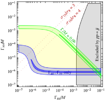
The prefered width to fit the ATLAS data is 45 GeV. However, most models of the $\Phi$ give much smaller total widths and also $BR(\Phi\to\gamma\gamma)\sim 10^{-3}-10^{-2}$. The range of possible values for $\Gamma(\Phi\to\gamma\gamma)$ and $\Gamma(\Phi\to gg)$ is illustrated in Fig. 1 [16]. The lower purple band represents the situation in which $gg$ and $\gamma\gamma$ decays dominate the total width of the $\Phi$. The upper green band corresponds to the situation that the total width of the $\Phi$ is indeed 45 GeV. In this paper, we will adopt the conservative assumption that $\Gamma(\Phi\to\gamma\gamma)$ is given by (5). The possibility that the 2-photon width of the $\Phi$ could be as large as 1 GeV is interesting for ILC, but, in our opinion, this is not likely. The preferred large width could also result from a model in which the $\Phi$ is actually formed as the sum of two nearby resonances. We will discuss this possibility in Section 3.2.

A useful phenomenological description of the coupling of $\Phi$ to $gg$ and $\gamma\gamma$ is given by the effective Lagrangian

$${\cal L}={\alpha_{s}\over 4}A_{3}\,\Phi\,G_{\mu\nu}G^{\mu\nu}+{\alpha_{w}\over 4}A_{2}\,\Phi\,W_{\mu\nu}W^{\mu\nu}+{\alpha^{\prime}\over 4}A_{1}\,\Phi\,B_{\mu\nu}B^{\mu\nu}\ ,$$ (6)

where $G$, $W$, $B$ are the field strengths of the $SU(3)$, $SU(2)$, $U(1)$ gauge fields of the SM and $\alpha_{s}$, $\alpha_{w}$, $\alpha^{\prime}$ are the corresponding coupling constants. We have written this Lagrangian for a scalar $\Phi$; for a pseudoscalar, substitute $F\tilde{F}$ for $F^{2}$. The constants $A_{i}$ have the dimensions of (mass)^-1 and indicate the scale of the new interactions that give rise to the coupling.

There is an important point to be emphasized here: The gauge symmetries of the Standard Model imply that any coupling of $\Phi$ to $gg$ or $\gamma\gamma$ must be through a non-renormalizable operator whose coefficient introduces a new mass scale. This implies the presence of new physics at that scale. This is the same argument by which the Fermi interaction implies new physics—the electroweak interaction—at the 100 GeV mass scale. Another example is given by the 125 GeV Higgs boson, whose the coupling to $gg$ has a form similar to (6), with

$$A_{3}={1\over 3\pi v}\ ,$$ (7)

where $v$ is the Higgs vacuum expectation value, 246 GeV. This coupling is generated by the top quark loop diagram.

In this formalism, the tree-level expressions for the $\Phi$ partial widths are (for $m_{\Phi}\gg m_{W},m_{Z}$)

$$\Gamma(\Phi\to gg) = {\alpha_{s}^{2}\over 8\pi}A_{3}^{2}m_{\Phi}^{3}$$

$$\Gamma(\Phi\to\gamma\gamma) = {\alpha^{2}\over 64\pi}(A_{2}+A_{1})^{2}m_{\Phi}^{3}$$

$$\Gamma(\Phi\to\gamma Z) = {\alpha\alpha_{w}c_{w}^{2}\over 32\pi}(A_{2}-{s_{w}^{2}\over c_{w}^{2}}A_{1})^{2}m_{\Phi}^{3}$$

$$\Gamma(\Phi\to ZZ) = {\alpha_{w}^{2}c_{w}^{4}\over 64\pi}(A_{2}+{s_{w}^{4}\over c_{w}^{4}}A_{1})^{2}m_{\Phi}^{3}$$

$$\Gamma(\Phi\to W^{+}W^{-}) = {\alpha_{w}^{2}\over 32\pi}A_{2}^{2}m_{\Phi}^{3}\ ,$$ (8)

where $(c_{w},s_{w})=(\cos\theta_{w},\sin\theta_{w})$. The value (5) implies

$$(A_{2}+A_{1})\sim 1/(500~{}\mbox{GeV})\ .$$ (9)

The structure of (8) implies that the $\Phi$ must decay either to $\gamma Z$ or to $ZZ$. Most likely, it decays to both channels, with branching ratios comparable to the rate to $\gamma\gamma$. Because the $Z$ is most convincingly seen at the LHC in its decay to $\ell^{+}\ell^{-}$ with a branching ratio of 7%, it is consistent with current data that these decays have not yet been seen. The fact that no resonance at 750 GeV has been observed in $WW$ and $ZZ$ at the LHC implies a relatively weak limit $A_{2}/A_{1}<12$ [22]. If the $\Phi$ is confirmed, we would expect that its $\gamma Z$, $ZZ$, and $W^{+}W^{-}$ decay modes would be observed at the LHC, and that these observations would clarify the effective Lagrangian (6).

Another piece of the evidence on $\Phi$ comes from the fact that it is not observed in other possible decay channels. Limits on $\Phi$ production at 8 TeV are collected in [15, 16, 17, 18, 23]. A particularly useful summary can be found in Table 1 of [16]. A result of particular significance here is that the $\Phi$ is not observed as a resonance in Drell-Yan production ($e^{+}e^{-}$ or $\mu^{+}\mu^{-}$), with a cross section upper bound comparable to the rate (2) for production in $\gamma\gamma$ [24]. A spin 0 $\Phi$ would not be expected to decay to light leptons, but this is possible in principle if the $\Phi$ has spin 2. If $BR(\Phi\to e^{+}e^{-})$ has a value not far below the current upper bound, then the $\Phi$ could appear as a prominent resonance in $e^{+}e^{-}$ at 750 GeV. We will discuss the significance of the $\Phi ee$ coupling in Section 3.6. Similarly, the $\Phi$ is not observed as a resonance in $t\overline{t}$ at a level corresponding to $BR(\Phi\to t\overline{t})/BR(\Phi\to\gamma\gamma)<450$ [25]. This can be a significant constraint for models that predict that $t\overline{t}$ is the dominant decay mode of the $\Phi$.

Beyond the question of the observable properties of the $\Phi$ lie important physics issues. In principle, the $\Phi$ could live in its own sector of particles, completely disjoint from the known Higgs boson. But, it is highly suggestive that the $\Phi$ is somehow related to the 125 GeV Higgs boson, or to other particles of the Standard Model. Thus, it is compelling to ask: Does the $\Phi$ resonance shed light on the origin of electroweak symmetry breaking, or on other mysteries associated with the TeV energy scale?

If this is the question, measurements at the ILC are likely to give an important part of the answer. Through its program of precision measurements, the ILC gives sensitivity to a very wide variety of new particles with masses below a few TeV. In particular, these measurements can discover effects from almost any new particle that affects the 125 GeV Higgs boson or the top quark. Thus, the ILC will allow us to ask directly whether there is a connection between the new and mysterious $\Phi$ resonance and the more familiar particles at the 100 GeV mass scale.

3 Imprint of the $\Phi$ on precision observables

In this section, we will make more concrete how to obtain information on the nature of the $\Phi$ from precision measurements that the ILC will make available. Many types of models have been proposed for the $\Phi$. In almost all of these, the $\Phi$ is accompanied by other types of new particles. The proposed models cover the whole range from weakly coupled models of extended Higgs sectors to strongly coupled models in which the $\Phi$ is composite. Each model is built on a specific, unique relation between the $\Phi$, the 125 GeV Higgs boson, and other new particles postulated in the model.

There is no model-independent analysis that makes these relations clear. Instead, it is necessary to examine the models one by one, understanding, in each case, the characteristic structure of the model and the impact predicted from this structure on known particles of the Standard Model. In this section, we will describe the various classes of models proposed for the $\Phi$ and clarify these relations in each case. We will also point out, for each class of models, the specific effects that should be visible in ILC measurements. We will cite explicit realizations of models of each class. A more complete bibliography of the literature on the $\Phi$, which now includes more than 400 theoretical papers, can be found in [26].

The literature on the $\Phi$ has shown that essentially every approach to new physics at the TeV scale can accomodate the $\Phi$, either by identifying the $\Phi$ with a particle already present in the model or by adding the $\Phi$ in a simple way. In models of the first type, the parameter values needed to include the $\Phi$ are often quite different from those anticipated prior to the $\Phi$ observation. In both cases, the new parameters often seem fine-tuned. In the discussion below, we simply accept these unusual or tuned parameters as the price of describing the $\Phi$ successfully.

In most cases, the existing literature on the implications of precision Higgs, top, and electroweak couplings already suggests methods by which measurement of these couplings can distinguish models of the various classes. Typically, the parameter choices needed to accomodate the $\Phi$ lead to effects in the precision measurements that are larger than those implied by generic choices.

3.1 Singlet coupling to vectorlike quarks and leptons

The simplest models of the $\Phi$ build a minimal structure around the effective Lagrangian (6). In these models, the $\Phi$ is a scalar or pseudoscalar Standard Model singlet. We must couple this state to heavy particles that can generate (6) when they are integrated out. To obtain sufficiently large couplings $A_{i}$, these heavy particles must, in most models, be fermions rather than scalars. It is not possible to use conventional 4th-generation quarks and leptons. For example, any heavy quark that obtains its full mass from the 125 GeV Higgs boson gives a contribution to the $hgg$ amplitude equal to that of the top quark. A heavy fourth-generation quark doublet would then increase the $hgg$ couplings by a factor 3 and the cross section $\sigma(gg\to h)$ by a factor 9. To generate (6) without such large effects on the 125 GeV Higgs, the heavy fermions should have the same $SU(2)\times U(1)$ quantum numbers for their left- and right-handed components, so that they can obtain mass without invoking the Higgs field expectation value. Such fermions are said to be “vectorlike”. In some models, the heavy fermions obtain mass from the vacuum expectation value of the field that gives rise to the $\Phi$ [15, 16, 17, 27, 28, 29, 30, 31, 32, 33].

To generate couplings both to gluons and to photons, the heavy particles must include states with both QCD and electroweak quantum numbers. In the simplest model, both types of couplings are generated by a heavy vectorlike quark. However, it is also possible that the gluon and electroweak couplings are generated by different particles, and, in particular, that the couplings to the photon are generated by new heavy leptons.

As an example, consider adding to the Standard Model a vectorlike heavy quark $Q$. This quark would couple to a scalar $\Phi$ via a Yukawa coupling

$${\cal L}\subset\ (m_{\Psi}+y\Phi)\overline{Q}Q\ .$$ (10)

(If $\Phi$ is a pseudoscalar, substitute $\overline{\Psi}\gamma^{5}\Psi$ in the second term.) The contributions to the $A_{i}$ in (6) are proportional to $y/m_{\Psi}$. For example, introduce a color-triplet, weak-singlet vectorlike quark of electric charge $5/3$. A calculation similar to (7) gives

$$A_{1}={50\over 9}{y\over\pi m_{Q}}\ ,\quad A_{2}=0\ ,\quad A_{3}={1\over 3}{y\over\pi m_{Q}}\ .$$ (11)

From the production cross section (2), we infer $m_{Q}/y\sim 900$ GeV. Then $y$ would lie in the interval between $y\sim 0.7$, where $Q$ should already have been discovered at the LHC, and $y\sim 4$, at which the coupling is so large that perturbation theory no longer applies. Then $Q$ can probably be discovered at the LHC with 3 ab^-1, except at the largest allowed values of $y$. In a model with several heavy vectorlike quarks, each contributes according to (11), and the estimated masses are larger.

Another possible case is generated by adding a vectorlike color octet fermion $G$ with zero electroweak quantum numbers and a vectorlike lepton $E$ with $(I,Y)=(0,1)$. In this case

$$A_{1}={2y_{E}\over\pi m_{E}}\ ,\quad A_{2}=0\ ,\quad A_{3}=2{y_{G}\over\pi m_{G}}\ .$$ (12)

In this case, the masses of $G$ and $E$ are not coupled in the phenomenology. The mass of $G$ can easily be above 3 TeV, beyond the reach of the LHC. The mass of $E$ should be below 1 TeV. The LHC can discover the $E$ in some but not all of this range. The paper [34] studies many possible decay schemes for the $E$ and computes expected limits from the High-Luminosity LHC ranging from 200 GeV to 500 GeV.

If $\Phi$ is a scalar, the theory must explain the absence of order-1 mixing between $\Phi$ and the SM doublet Higgs $H$, which is constrained by LHC measurements. To achieve this, one can postulate a $Z_{2}$ symmetry under which $\Phi$ is odd and $H$ is even. However, the Yukawa coupling in (10) breaks this symmetry, inducing the doublet-singlet mixing through radiative corrections. This mixing in turn induces shifts in the couplings of the 125 GeV Higgs boson to gluons and photons, typically in the $1-10$% range accessible at the ILC. Interestingly, the presence of the extra scalar in this model may induce a strongly first-order electroweak phase transition, opening the possibility of electroweak baryogenesis [35]. In this scenario, Higgs couplings to photons and gluons must deviate by $5-10$% from their SM values.

Heavy vectorlike fermions are welcome in many theories of physics beyond the Standard Model. This is especially true for vectorlike quarks. In Little Higgs theories [36, 37, 38] and certain versions of the Randall-Sundrum model [39], vectorlike quark with charge $2/3$—top quark partners—cancel the divergence in the Higgs boson mass coming from top quark loops and thus are a crucial ingredient in solving the hierarchy problem. Top partners that play this role typically also mix with the top quark, inducing shifts in the top quark couplings to the weak gauge bosons. ILC measurements of the top width and its couplings to the $Z$ are sensitive to these effects throughout the natural region of parameter space in these models [40].

Another possibility is that the $\Phi$ and the vectorlike fermions arise within a grand unified theory. For example, adding extra ${\bf 5}+{\bf\overline{5}}$ representations to standard $SU(5)$ grand unification adds vectorlike fermions whose masses do not depend on the Higgs field vacuum expectation value. An interesting and quite predictive example is given in [41]. This is a supersymmetric model which introduces ${\bf 5}+{\bf\overline{5}}$ multiplets that obtain mass from a the vacuum expectation value of a complex field $S$. The new multiplets give rise to vectorlike quarks with $(I,Y)=(0,-\frac{1}{3})$ and vectorlike leptons with $(I,Y)=(\frac{1}{2},-\frac{1}{2})$. The assumption of unification at the GUT scale, plus renormalization group running, fixes the masses of these particles to be in the ratio 2.5:1. The overall mass scale is related to the size of the coefficients in the effective Lagrangian (6). The leptons expected to have masses below 400 GeV, accessible for detailed study at least at an energy-upgraded ILC.

Figure 2: Expected exclusion of vectorlike leptons by precision measurement of the cross sections for $e^{+}e^{-}\to\mu^{+}\mu^{-}$ and $e^{+}e^{-}\to e^{+}e^{-}$ at the ILC at 500 GeV with 1000 ab^-1 of data, from [42], as a function of mass and multiplicity times squared charge. The figure is shown for leptons with $I=Y=\frac{1}{2}$. The colored bands show the region of the plane that generates a $\Phi$ signal cross section of 3–10 fb, for the three values $y=0.1,0.3,1$.

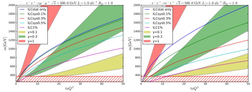
The ILC can give evidence for heavy fermions not only through direct production but also, indirectly, through the effect of these particles on the $U(1)$ and $SU(2)$ vacuum polarization amplitudes, which can be extracted from precision measurement of 2-fermion scattering. Figure 2 gives an example [42]. In the figure, the area below the curves can be excluded by ILC measurements of and $e^{+}e^{-}\to\mu^{+}\mu^{-}$ and $e^{+}e^{-}\to e^{+}e^{-}$ at 500 GeV with polarized electron beams $(P_{e^{-}},P_{e^{+}})=(-80\%,30\%)$ and 1 ab^-1 of data. (The actual ILC run plan expects 4 ab^-1 of data at 500 GeV, divided among several combinations of beam polarization [12].) The colored bands show the regions of fermion mass and charge predicted for a $\Phi$ signal of 3-10 fb. It should be noted that models with ${\mbox{\rm tr}}[Q^{2}]>6.7$ are inconsistent with standard grand unification, since some coupling run to large values (or a Landau pole) below the GUT scale. Still, such large values are possible in a more general model context. It is interesting that the vacuum polarization measurement can be sensitive to fermions with masses well above 1 TeV.

3.2 Extended Higgs sector

The models discussed in the previous section introduce the minimal structure needed to account for the $\Phi$ and the effective Lagrangian (6). In this section, we will discuss models that extend these ideas by postulating a specific relation of the $\Phi$ and the 125 GeV Higgs boson within an extended Higgs sector of fields.

The simplest scheme involves adding a new singlet Higgs boson to the Standard Model Higgs doublet. This possibility is explored, for example, in [17, 28, 30, 43, 44, 45, 46]. Heavy vectorlike fermions, as described in the previous section, are needed to provide the effective Lagrangian couplings (6).

An $SU(2)$ singlet scalar boson has the same quantum numbers, after symmetry breaking, as the 125 GeV Higgs boson and, in general, cannot avoid mixing with the Higgs boson. Such mixing effects could appear in precision measurements of the Higgs boson properties. The mixing angle is limited by electroweak precision measurements to satisfy $\sin\theta<0.35$ for a singlet mass of 750 GeV [47]. A stronger limit, $\sin\theta<1\%$, comes from the fact that the $\Phi$ can decay to $ZZ$ through mixing with the Higgs, and this decay is bounded by observation [48]. The effect of this mixing on the $hWW$ and $hZZ$ couplings is at the $10^{-4}$ level, and thus probably unobservable. However, a mixing angle of this size would still produce percent-level effects in the $gg$ and $\gamma\gamma$ Higgs couplings. Also, if $\Phi$ couples to Standard Model fermions such as $b\overline{b}$ or $\tau^{+}\tau^{-}$, those couplings of $h$ could be shifted from their Standard Model values at the percent level. All of these effects would be tested in the ILC’s comprehensive program of Higgs boson coupling determinations.

An interesting possibility raised by [45] is that a neutral heavy vectorlike fermion could be the particle of dark matter. The $\Phi$, if it is a scalar, not a pseudoscalar, would provide an s-channel resonance in fermion pair annihilation that would allow the fermions to have the correct thermal relic density for masses in the range $300<m_{\psi}<450$ GeV. Such particles would be extremely difficult to discover at the LHC, but they would be seen in the reaction $e^{+}e^{-}\to\gamma\psi\overline{\psi}$ at the ILC operating an upgraded energy of 1 TeV [49].

Models of the $\Phi$ as the heavy $H,A$ states of a 2-Higgs-doublet model have been presented in [7, 18, 43, 50, 51, 52, 53]. Again, the natural couplings of these particles to $\gamma\gamma$ and $gg$ through Standard Model loops are too small to account for the observation, so new vectorlike fermions are also needed. Models of this type are constrained at large $\tan\beta$ by the non-observation at the LHC of $\Phi$ decays to $\tau^{+}\tau^{-}$ and at small $\tan\beta$ by the non-observation of decays to $t\overline{t}$. These constraints lead to a preference for intermediate values of $\tan\beta$, close to $\tan\beta\sim 7$. This places the models in the “wedge” region of the 2-Higgs-doublet model in which it is very difficult for the LHC to observe the heavy Higgs bosons beyond masses of 500 GeV through more conventional processes such as $b\overline{b}\to H,A\to\tau^{+}\tau^{-}$. The enhanced $gg$ coupling of the $\Phi$ gives a new production mechanism, but still it might not be seen to decay to heavy fermions.

On the other hand, the 2-Higgs doublet model requires mixing of the heavy Higgs bosons with the 125 GeV Higgs boson, producing shifts in the $\tau\tau$ and $b\overline{b}$ couplings of the known Higgs boson. Observation of these effects of heavy $H,A$ bosons of mass 750 GeV are expected [54] to be well within the 5 $\sigma$ reach of the full ILC program described in [11].

An interesting possibility in the 2-Higgs-doublet model is that the $H$ and $A$ could be close in mass, so that the $\Phi$ resonance is actually a double resonance, one scalar and one pseudoscalar particle. If the mass difference of these particles is of the order of tens of GeV, this might explain the broad width required in the best fit to the ATLAS data. This scenario can also be realized in models with $SU(2)$ singlets only [55]. It is possible that the two separate resonances could be resolved with higher-statistics $\gamma\gamma$ observations at the LHC. However, the crucial test of this model would come in the photon collider experiments described below in Section 4.4. Using transversely polarized photon beams, the shape of the resonance would shift as the relative beam polarizations were switched from parallel to orthogonal orientations.

The $\Phi$ has also been interpreted as one of the heavy Higgs bosons in the NMSSM extended supersymmetric model [55, 56, 57, 58]. Here, it is possible to choose parameters such that the LHC production is through $b\overline{b}$ annihilation and the Higgsinos play the role of the heavy vectorlike fermions in generating a coupling to $\gamma\gamma$. Generally, for these parameters, the mass of the Higgsino is typically close to $m_{\Phi}/2$, making Higgsino pairs discoverable at a 1 TeV energy upgrade of the ILC; however, for some parameter sets, the Higgsinos can be as light as 150 GeV.

One property of NMSSM models, emphasized in [56, 58], is that the decay of the $\Phi$ can be to very light Higgs states $a$, with mass close to the $\pi^{0}$ mass, each of which then decays to $\gamma\gamma$. The apparent $\Phi\to\gamma\gamma$ decay would then actually be a decay to two $\gamma$ pairs of very low mass. It is unavoidable that the 125 GeV Higgs boson also has the decay $h\to aa$ at some level, and the current limit on the branching ratio of the Higgs boson to this mode, about 1%, is already a constraint on the models. The High-Luminosity LHC is expected to be sensitive to a branching ratio as small as $5\times 10^{-5}$ [59]. ILC can add to the information on $h\to aa$, since it will be sensitive to decays of the $a$ to hadrons that might be hidden at LHC.

Two Higgs doublet models have also been introduced to explain a different aspect of the LHC data, the suggestion by CMS of a decay $h\to\tau\mu$ [60]. The second Higgs doublet has no couplings to fermions except through small flavor mixing effects. In [53], the heavy Higgs scalar in this model is interpreted as the $\Phi$ and appropriate heavy vectorlike fermions are added to produce the effective Lagrangian couplings (6). It is obvious that, if the CMS suggestion is confirmed, measurement of the detailed structure of Higgs flavor violation—both in the quark and lepton sectors—will be a major task for the ILC. In addition, mixing between the two doublets will shift the absolute normalizations of the flavor-diagonal Higgs couplings, an effect that ILC can probe below the 1% level.

3.3 Bound state of new weakly-coupled constituents

It has been appreciated for a long time that the top squark might first be identified through the decay of stoponium to $\gamma\gamma$ [61, 62, 63]. Pursuing these ideas, several authors have interpreted the $\Phi$ as a nonrelativistic bound state of new fermions or bosons [64, 65, 66, 67, 68, 69, 70]. Stoponium itself has a signal cross section about 10 times too small, but this can be overcome by assuming larger electric charge (e.g., $5/3$) for the constituents.

In these models, the continuum production of the new particles should be discovered at the LHC. The effects in precision measurements are small, precisely because these models are constructed to isolate the $\Phi$ from other physics at the TeV scale. At the very least, the vacuum polarization corrections from the new particles will produce shifts of order 1% in the cross sections for $e^{+}e^{-}\to\mu^{+}\mu^{-}$ and $e^{+}e^{-}\to e^{+}e^{-}$, as we have discussed in a more general context at the end of Section 3.1. If the new heavy particles have direct couplings to $t$ or $b$, we will see effects on the Higgs boson and top quark similar to those described above for heavy vectorlike fermions.

3.4 Pion of a new strong interaction sector

A very different picture of the origin of a new scalar or pseudoscalar comes from models with new strong interactions at multi-TeV energies. The new strong interactions might involve a sector of heavy fermions charged under a confining non-Abelian gauge group. Such theories quite naturally contain spontaneously broken global chiral symmetries. These lead to (pseudo-) Nambu-Goldstone bosons (pNGB, generically also called pions), that are naturally light by the Goldstone mechanism. The $\Phi$ could be one of these pions. It is useful to think of it as analogous to the $\eta$ or $\eta^{\prime}$ of QCD. In many of these models, additional pNGBs are expected to have masses with the reach of the LHC, giving the potential to further constrain the model space. If the $\Phi$ comes from a decay of another resonance with mass larger or equal than 1500 GeV [13, 14, 15], we might already have evidence for one of these states.

The fermions of the new gauge group must be charged under the QCD and electroweak gauge groups in order that the $\Phi$ will have the effective Lagrangian couplings (6). If this is so, the model generates these couplings in the same way that QCD generates an $\eta\to\gamma\gamma$ coupling [71, 72, 73, 74]. The precise prediction for the rates and decay patterns of these fermions depend on the specific model, particularly the confining gauge group (usually assumed to be some $SU(N)$), the fermion content and its quantum numbers. Some classification has been done, using assumptions on minimal flavor violation, the absence of Landau poles in the gauge couplings as well as the existence of maximally two diphoton candidates in the models. Still, the model space is vast. Generically, all kinds of these models, which could be composite Higgs models, models of partial compositeness, Little Higgs models or even Twin Higgs models, are all having particular patterns of deviations in the Higgs (and also top) couplings. Their measurements – using the information on the diphoton resonance gathered at the LHC – will be an indispensable tool in determining the specific underlying model.

There is an interesting connection with dark matter. In models of dark matter based on models with new strong interactions, the dark matter particle is typically, the lightest pNGB. The width of the $\Phi$ can be enhanced substantially by invisible decays to pairs of dark matter pNGBs. If indeed this effect enhances the width of the $\Phi$, giving better agreement with the current observations, it argues that the dark matter particle lies below half the $\Phi$ mass and potentially in the energy range of the ILC. For an isolated $\Phi$ resonance, the thermal relic abundance of dark matter is correct for a dark matter mass of about 300 GeV. If there are two pNGBs close in mass, so that the relic abundance is set by coannihilation, dark matter masses lower than 100 GeV are favored, and the dark matter pair threshold would be within the range of the 500 GeV ILC [72].

3.5 Radion of Randall-Sundrum models

A more concrete model representing effects of new strong interactions at the TeV energy scale is the Randall-Sundrum (RS) model [75]. In this model, our 4-dimensional space is extended to a 5-dimensional warped space with 4-dimensional boundaries. Due to the warping of space, excitations on the boundaries naturally have different energy scales. These boundaries are called, accordingly, the IR and UV branes. The IR scale is typically about 1 TeV. Fields in the 5-dimensional interior give rise to a spectrum of quantum excitations, called Kaluza-Klein (KK) excitations. The spectrum of these KK states extends to infinity, forming the so-called “Kaluza-Klein tower”; however, the lowest-mass states typically give the dominant contributions to observable effects. The RS model can be considered a dual description of a strong-interaction theory above 1 TeV, with the KK excitations modelling the strong interaction bound state spectrum. Or, the RS model can be thought of as a 5-dimensional theory of electroweak symmetry breaking in its own right.

The RS model contains a special new scalar particle called the radion. The radion is a quantum excitation of the position of the IR brane in the 5th dimension. In models such as those of [76, 77, 78], the mass of this radion can be of the order of 500 GeV, making it reasonable to associate this particle with the $\Phi$. The phenomenology of the radion depends on the arrangement of Standard Model and new fields in the 5-dimensional space. The placement of these fields in the interior or on the boundary is a matter of model-building, but it is also constrained by electroweak precision data and the lack of observation, so far, of Standard Model KK excitations at the LHC. A typical property of the radion is that it has a large coupling to $t\overline{t}$, leading to a large $\Phi\to t\overline{t}$ event rate. The models just cited find parameter sets that avoid this problem.

There is another type of new particle also predicted in the RS model. KK excitations of gravity in the 5-dimensional interior can have couplings of electroweak strength to some Standard Model particles. It is possible to build models in which the lightest new particle in an RS model is a spin 2 KK excitation of the graviton. This gives a different theory of the $\Phi$ that we will discuss in the next section.

Three effects on ILC precision measurements are expected if there is an RS extension of the Standard Model that gives the $\Phi$ as a radion. The first of these effects is Higgs-radion mixing. The radion is an $SU(2)$-singlet state, and so the phenomenology of this mixing is similar to that discussed for a singlet Higgs boson in Section 3.2. Often, the mixing angle is very small; for example, [77] estimates $\theta_{m}\sim m_{h}^{2}/6m_{\Phi}^{2}\sim 0.5\%$. This removes the possibility of observing shifts in the overall level of Higgs couplings, which are proportional to $\cos\theta_{m}$, but large couplings of the radion to $gg$ and $\gamma\gamma$, which give $\sin\theta_{m}$ shifts of these particular Higgs couplings, should still be observable.

The second effect is that of corrections from the tower of KK states to the Higgs boson couplings to heavy species $W$, $Z$ and $t$. The masses of the lowest KK states are model-dependent, ranging from a few TeV to tens of TeV. However, even at the heavier values, the radiative corrections to the Higgs couplings can be substantial. For example, the models of [79] predict shits of the Higgs boson couplings to vector bosons $c_{V}=g(hVV)/g(hVV)|_{SM}$ of the form

$$c_{W}\approx c_{Z}\approx 1-0.078\left({5\ \mbox{TeV}\over M_{g(1)}}\right)^{2}.$$ (13)

where $M_{g(1)}$ is the mass of the first Kaluza-Klein excitation of the gluon. For a 5 TeV Kaluza-Klein excitation this leads to an $\sim$8% deviation. With the formula (13), even a 20 TeV KK gluon would produce observable effects, for both $W$ and $Z$, in the ILC precision measurements.

The top quark Yukawa coupling should also receive large radiative corrections from the KK towers of states. Figure 3 shows the shifts of the Higgs boson couplings computed in [79] for a variety of parameters sets, as a function of the mass of the lightest KK gluon. Note that these shifts are in general complex, leading to CP violation in the $ht\overline{t}$ coupling at levels observable at the ILC [80]. The figure shows the shifts as parameters $c_{t}$, $c_{t5}$ corresponding to the effective coupling

$$\delta{\cal L}=-{m_{t}\over v}\ h\ \bigl{[}c_{t}\ \overline{t}t+ic_{t5}\ \overline{t}\gamma^{5}t\bigr{]}.$$ (14)

Figure 3: Predictions of $CP$-even (left) and $CP$-odd (right) Higgs couplings to the $t$ quark in a Randall-Sundrum model with a custodial symmetry. The parameters $c_{t}$, $c_{t5}$ are defined in (14). The point clouds are a scan of the space of Yukawa couplings for three values of the free parameter $y_{\ast}$. The gray band on the right hand side shows the experimental bound at 90% on the CP-odd predictions derived from the electron dipole moment (EDM). Figure and parts of the caption are taken from [79].

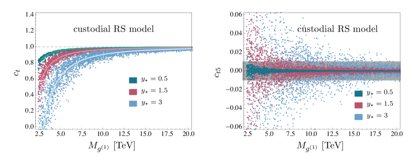
The third effect is a modification of the electroweak couplings of the top quark. In RS models, the top quark wavefunction extends to the IR side of the 5th dimension, and so the top quark shares some of the compositeness of the Higgs boson. In particular, while the wavefunctions of light fermions peak close to the UV brane, the wavefunction of the $t_{R}$ often peaks close to the IR brane. This may constitute an elegant explanation of the striking mass hierarchy in the fermion sector. A consequence of this effect is that the couplings of the top quark to the $Z$ boson are expected to have large shifts due to mixing with KK states, of independent size for $t_{L}$ and $t_{R}$. Models of this effect are described, for example, in [81, 82].

One of the well-appreciated features of the ILC is that the $t\overline{t}Z$ couplings enter the expressions for the production of top quark pairs in $e^{+}e^{-}\to t\overline{t}$. The couplings to $t_{L}$ and $t_{R}$ can be separately measured using polarized beams [83]. In [11], these measurements are reviewed, and errors of order 1% on the separate $Z$ couplings to $t_{L}$ and $t_{R}$ are estimated for the full ILC program. As discussed there, these accuracies suffice not only to observe the effect but also to provide significant discrimination among models.

3.6 Graviton of Randall-Sundrum models

The $\Phi$ resonance could be a particle of spin 2 rather than a particle of spin 0. At the LHC, the spin of the resonance can be determined by studying the angular distribution of the photons. Demonstrating that the photon distribution in the rest frame of the diphoton system is not isotropic, but instead is strongly peaked in the beam axis direction, would be a smoking gun for the spin-2 nature of the resonance.

One example of a theory that provides a spin-2 resonance with properties of the $\Phi$ is the Randall-Sundrum (RS) model [75], in the region of parameter space where the lightest KK graviton excitation is the lightest new particle. By the introduction of additional interactions on the 4-dimensional boundaries of the warped space, it is possible to realize parameters in which the KK graviton is lighter than the RS radion excitation described in the previous subsection. In such a construction, there is a danger that the radion may become a negative-metric (ghost) particle; however, the papers cited below find parameter sets that avoid this problem.

A key issue relevant to the interpretation of the $\Phi$ as an RS graviton is the question of whether the resonance couples to $e^{+}e^{-}$ pairs. In the simplest scenario, the entire Standard Model is localized on the IR brane [84]. In this case, the $\Phi$ would couple to the energy-momentum tensor of the Standard Model and thus would couple with the same strength to $e^{+}e^{-}$ and $\mu^{+}\mu^{-}$ as to $\gamma\gamma$. Then the $\Phi$ would be expected to appear as a resonance in the Drell-Yan process. This is not observed and, while this model is not yet excluded, it provides a nontrivial constraint. However, it is also possible to have non-universal couplings of the spin-2 resonance to the SM if one allows the SM fields to also propagate in 5 dimensions. In a construction of this type, lighter quarks and leptons have 5-dimensional wavefunction localized further from the IR brane. This leads to smaller Yukawa couplings and smaller fermion masses; thus, the construction can be used to address the fermion mass puzzle. Wavefunctions further from the IR brane also couple less strongly to the lowest KK graviton excitations, thus relaxing the constraint from the Drell-Yan process [85, 86, 87, 88].

The RS graviton couples to photons and gluons, and the parameters of the model can be adjusted to correctly reproduce the LHC observations of the diphoton resonance. Other decay modes should also be observed. In particular, if the RS framework plays a role in addressing the hierarchy problem, also $WW$, $ZZ$, $hh$, and $t\overline{t}$ decays are expected to occur with a significant branching fraction. Table 1 shows the KK graviton branching fractions in several benchmark models, including the IR model from [84] and four models with SM fields in the bulk defined in [85].

	IR	MIN	MED	MAX	GMAX
${\rm Br}(X\to\gamma\gamma)$ [%]	4.3	8.5	7.0	0.5	2.3
${\rm Br}(X\to ZZ)$ [%]	4.8	7.9	7.8	2.9	12
${\rm Br}(X\to WW)$ [%]	9.5	16	15	5.6	21
${\rm Br}(X\to Z\gamma)$ [%]	0	0	0	0	1.1
${\rm Br}(X\to hh)$ [%]	0.3	0	0.4	1.4	6.9
${\rm Br}(X\to t\overline{t})$ [%]	5.1	0	8.3	85	56
${\rm Br}(X\to b\overline{b})$ [%]	6.4	0	5.2	0.4	0.04
${\rm Br}(X\to jj)$ [%]	66	68	61	4.5	0.5
${\rm Br}(X\to e^{+}e^{-})$ [%]	2.1	0	0	0	0
$\Gamma(X\to\gamma\gamma)$[MeV]	0.25	0.15	0.18	2.5	25
$\Gamma(X\to{\rm tot})$[MeV]	5.7	1.8	2.6	500	1060
PLC: $\sigma_{eff}(\gamma\gamma\to X)$ [fb]	40	24	29	400	4000
LC: $\sigma(e^{+}e^{-}\to X)$ [pb]	0.4	0	0	0	0

Table 1: Observables for the IR model defined in Ref. [84] and for the MIN, MED, MAX, and GMAX benchmarks in the bulk RS scenario defined in Ref. [85].

From this discussion, we see that the size of the coupling of the $\Phi$ to $e^{+}e^{-}$ is a key test that discriminates RS models on the basis of the localization of wavefunctions in the 5th dimension. We have pointed out in Section 2 that the $\Phi$ coupling to $e^{+}e^{-}$ is constrained by the non-observation of the $\Phi$ in the Drell-Yan spectrum, but it could still be comparable to the $\gamma\gamma$ coupling. Thus, the possibility is open that the $\Phi$ could be observed as a resonance in $e^{+}e^{-}$ collisions.

One might hope that, in $e^{+}e^{-}$ collisions at 500 GeV, the $\Phi$ might be observable as a spin-2 contact interaction in $e^{+}e^{-}\to\gamma\gamma$ or $b\overline{b}$. Unfortunately, for the models in Table 1, the effects on the angular distributions in the 2-body final state are at most of the order of $10^{-4}$. However, the presence of an RS model at 1 TeV will be recognizable at the ILC, since it will produce the spectrum of effects on precision measurements described in the previous section.

With an energy upgrade of the ILC to 1 TeV, it will be possible to explore for the $\Phi$ resonance in $e^{+}e^{-}$ annihilation more directly. We will discuss the phenomenology of a spin-2 $\Phi$ resonance in Section 4.5.

3.7 Summary

The discussion of this section is summarized in Table 2. For each of the models that we have discussed in this section, we mark in this table the precision Higgs, top or $e^{+}e^{-}$ measurement available from the ILC in which a significant deviation from the Standard Model would be expected. The observation of these anomalies would put us on the right path toward building concrete theories to explain the $\Phi$. The values of the anomalies will fix explicit parameters in these theories. More information would be available if the anomalies observed at the ILC could be correlated with the properties of new particles discovered at the LHC. We hope for such discoveries, but the discovery of further new particles at the LHC is not guaranteed in any scenario. The table makes clear that, independently of any further information from the LHC, precision measurements at the ILC will give many new pieces of information on the origin and nature of the $\Phi$ resonance.

Sect.		$hWW$	$hb\overline{b}$	$h\gamma\gamma$	$ht\overline{t}$	$h\to$	$h\tau\mu$	$t\overline{t}Z$	$ee\to$	$ee\to$
		$hZZ$	$h\tau\tau$	$hgg$		invis.			$ee,\mu\mu$	$\gamma+$ invis.
3.1	Vectorlike
	fermions		X	X	X			X	X
3.2	Higgs
	singlet		X	X	X			X
3.2	2 Higgs
	doublet	X	X	X	X
3.2	NMSSM
		X	X	X	X	X				X
3.2	Flavored
	Higgs	X	X	X			X
3.3	Bound
	state								X
3.4	Pion of
	new forces		X	X	X	X		X	X	X
3.5	RS
	radion	X	X	X	X			X
3.6	RS
	graviton	X	X		X			X

Table 2: Anomalies in precision measurements expected to be visible at the ILC for the models of the $\Phi$ discussed in Section 3 of this report.

4 Observation of the $\Phi$ in $\gamma\gamma$ and $e^{+}e^{-}$ collisions

Up to this point, we have been discussing only tests of theories of the $\Phi$ available at energies of 500 GeV and below. However, the ILC TDR also envisioned an energy upgrade to 1 TeV [89]. This upgrade would give the possibility of producing the $\Phi$ directly. Since the $\Phi$ is observed in the decay $\Phi\to\gamma\gamma$, at least one of the couplings $A_{1}$ or $A_{2}$ in (6) must be nonzero. Then there are nonzero cross sections for production of the $\Phi$ both in $e^{+}e^{-}$ and in $\gamma\gamma$ collisions. If the $\Phi$ resonance can be observed, these processes will give access to the full range of decay modes of the resonance, just as the ILC is expected to allow the study of the full set of decay modes of the 125 GeV Higgs boson.

Four distinct processes can be studied. First $\Phi$ can be produced from $e^{+}e^{-}$ beams via the associated production with $\gamma$ or $Z$,

$$e^{+}e^{-}\to\Phi V\ ,\quad\mbox{with}\quad V=\gamma,Z\ .$$ (15)

These processes can be characterized by the observation of a monochromatic electroweak gauge boson.

Second, $\Phi$ can be produced via the vector boson fusion processes [6]

$$e^{+}e^{-}\to\Phi e^{+}e^{-}\ ,\quad\Phi\overline{\nu}_{e}\nu_{e}\ .$$ (16)

These processes can be identified by the characteristic transverse momentum of order $m_{W}$ imparted to the $\Phi$. The reaction $e^{+}e^{-}\rightarrow\Phi e^{+}e^{-}$ is also likely to have energetic $e^{\pm}$ observed at small scattering angles.

Third, the ILC at 1 TeV can be used as the basis of a photon-photon linear collider (PLC). In this facility, the $\Phi$ would be produced in $\gamma\gamma$ collision [6, 7, 8, 9]

$$\gamma\gamma\rightarrow\Phi\ .$$ (17)

Finally, the possibility of a direct coupling of $\Phi$ to $e^{+}e^{-}$ raises the possiblity of observing the resonant production $e^{+}e^{-}\to\Phi$.

In this section, we will discuss the cross sections for $\Phi$ production and the possibility of $\Phi$ observation in these processes. The cross sections that we compute will be based on the effective Lagrangian (6) and will be proportional to $\Gamma(\Phi\to\gamma\gamma)$. For numerical estimates, we will use the conservative reference value $\Gamma(\Phi\to\gamma\gamma)=0.5$ MeV, as discussed below (5). We have pointed out in Section 2 and in Fig. 1 that the value of $\Gamma(\Phi\to\gamma\gamma)$ could potentially be three orders of magnitude larger than this value. In that case, the cross sections computed in this paper would be larger by the same factor. The reader should keep this in mind in evaluating the rate estimates that we present here.

4.1 $e^{+}e^{-}\rightarrow\Phi\gamma$ or $\Phi Z$

From the effective Lagrangian (6), it is straightforward to work out the cross section for $e^{+}e^{-}\rightarrow\Phi V$. These cross sections simplify dramatically in the limit $s/m_{Z}^{2}\gg 1$, which actually applies for $\sqrt{s}\geq 750$ GeV. In that limit, the polarized cross sections are

$${d\sigma\over d\cos\theta}={\alpha_{w}^{3}\over 32}|C|^{2}(1+\cos^{2}\theta)(1-m_{\Phi}^{2}/s)^{3}\ ,$$ (18)

where the coefficients $C$ are given by

$$C(e^{-}_{L}e^{+}_{R}\to\Phi\gamma) = \biggl{(}{s_{w}\over 2}A_{2}+{s_{w}^{3}\over 2c_{w}^{2}}A_{1}\biggr{)}$$

$$C(e^{-}_{R}e^{+}_{L}\to\Phi\gamma) = \biggl{(}{s_{w}^{3}\over c_{w}^{2}}A_{1}\biggr{)}$$

$$C(e^{-}_{L}e^{+}_{R}\to\Phi Z) = \biggl{(}{c_{w}\over 2}A_{2}-{s_{w}^{4}\over 2c_{w}^{3}}A_{1}\biggr{)}$$

$$C(e^{-}_{R}e^{+}_{L}\to\Phi Z) = \biggl{(}-{s_{w}^{4}\over c_{w}^{3}}A_{1}\biggr{)}$$ (19)

For $A_{2}\sim(500~{}\mbox{GeV})^{-2}$ as suggested by (5), this gives cross sections from the $e^{-}_{L}e^{+}_{R}$ state at $\sqrt{s}=1$ TeV of order of tens of ab, which is small but promises a finite sample of events. If higher energies are accessible, the cross section increases rapidly as $\beta\to 1$. In this approximation, the same cross section formulae apply for a scalar or a pseudoscalar $\Phi$, using for the pseudoscalar case the modified Lagrangian described in the text below (6).

The cross sections of processes $e^{+}e^{-}\to\Phi\gamma$ and $e^{+}e^{-}\to\Phi Z$ for different beam polarisations are shown in Fig. 4. These figures use the complete formulae [90, 91] rather than the approximations (18). The various curves in each figure correspond to different values of the parameter $R$ given by

$$R={A_{2}/A_{1}}\ ,$$ (20)

assuming the $\Phi\to\gamma\gamma$ partial width given in (5). (The results for the upper limit $R=12$ quoted in Section 2 are close to those for $R=\infty$.) The figures include the expected 80% electron beam polarization and 30% positron beam polarization.

The expected cross sections are small in the most conservative scenario. However, if a substantial event sample can be gathered, these processes potentially give a large amount of information about the $\Phi$. The most important feature is that the $\Phi$ can be tagged by the $\gamma$ or $Z$ recoiling against the $\Phi$ without any requirement on the $\Phi$ decay mode. The situation is similar to that for the Higgs boson in $e^{+}e^{-}\to Zh$. This allows us to determine the absoute partial widths $\Gamma(\Phi\to\gamma\gamma)$, $\Gamma(\Phi\to\gamma Z)$, and $\Gamma(\Phi\to ZZ)$, and, from these, the total width of the $\Phi$ and the branching ratios to any other observed decay channel. The recoil method is sensitive to $\Phi$ decays to invisible particles and to other exotic final states that are difficult to reconstruct.

The CP property of the $\Phi$ can be studied in $e^{+}e^{-}\to\Phi Z$, with $Z$ decaying hadronically. This might usefully supplement CP and spin information obtained from studies of $\Phi\to ZZ\to 4$ leptons at the LHC.

Figure 4: Total cross sections for the process $e^{+}e^{-}\to\Phi\gamma$, $e^{+}e^{-}\to\Phi Z$, for polarized beams, in ab, as a function of the collision energy. The different curves refer to different values of $R$ in (20): dashed: $R=\infty$ (pure $A_{2}$; solid: $R=1$; dotted: $R=0$ (pure $A_{1}$). In each case, the cross sections are computed assuming 80% electron beam polarization and 30% positron beam polarization. ISR and beamstrahlung are not included. These cross sections are based on a conservative value of $\Gamma(\Phi\to\gamma\gamma)$, as discussed in the text.

4.2 $e^{+}e^{-}\rightarrow\Phi e^{+}e^{-}$

The reaction $e^{+}e^{-}\rightarrow\Phi e^{+}e^{-}$ can proceed through $\gamma\gamma$ or $ZZ$ fusion. The leading contribution comes from $\gamma\gamma$ fusion with small scattering angles of the electron and positron, which can be estimated by using the equivalent photon approximation [92]. However, the resulting cross section are very low. We expect a total rate of 22 ab. To isolate the signal from background, it is useful to detect either or both of the $e^{-}$ and $e^{+}$ in forward detectors. If we require that at least one of the scattered particles has scattering angle larger than 10 mrad and energy larger than 50 GeV, we find a cross section of 8 ab. Requiring both the $e^{-}$ and $e^{+}$ to meet this criterion gives a cross section of 1 ab.

4.3 Interlude: PLC

If the $\Phi$ decays to $\gamma\gamma$, it must also be produced in $\gamma\gamma$ collisions. To observe this process with sufficient rate, the ILC should be converted to a Photon Linear Collider (PLC), by Compton backscattering of laser beams from the electron beams. Analyses of the $\Phi$ cross section in $\gamma\gamma$ in this setting have been given in [6, 7, 8, 9]. Useful background on the accelerator physics of a $\gamma\gamma$ collider can be found in the relevant volume of the TESLA TDR [5].

A useful figure of merit to understand the observability of the $\Phi$ is the size of $\Gamma(\Phi\to\gamma\gamma)/m_{\Phi}$, which can be compared to the similar ratio for the 125 GeV Higgs boson. The values are

$${\Gamma(\Phi\to\gamma\gamma)\over m_{\Phi}}\geq 7\times 10^{-7}\ ,\qquad{\Gamma(h\to\gamma\gamma)\over m_{h}}=7\times 10^{-8}\ .$$ (21)

Thus, we expect that the $\Phi$ will be easier to observe above background than the 125 GeV Higgs boson, whose production at a $\gamma\gamma$ collider has been studied in detail in [93].

A $\gamma\gamma$ collider would be based on a $e^{-}e^{-}$ operation of the ILC, at an energy about 25% higher than the energy of the $\Phi$ resonance. The most commonly discussed operating point for a $\gamma\gamma$ collider is at the parameter of the Compton scattering process

$$x={s_{e\gamma}\over m_{e}^{2}}=15.3\bigl{(}{E_{beam}\over\mbox{TeV}}\bigr{)}\bigl{(}{\omega\over\mbox{eV}}\bigr{)}$$ (22)

having the value $x=4.8$ [94]. For operation with a maximum $\gamma\gamma$ center of mass energy of 800 GeV, this requires a 1 TeV $e^{-}e^{-}$ collider and a laser of wavelength $2\mu$m and average power about 100 kW. The time structure of the laser must be matched to the time structure of the ILC beams. A possible solution to this problem is to construct an an optical cavity surrounding the ILC detector whose length is close to the time separation within a train of ILC pulses [95]. High-power lasers of 100 kW are available today at $1\mu$ wavelength. This would require working at value of $x$ that is acceptable though not optimal for the PLC. The technology of high-power lasers is advancing rapidly though, and it is likely that a laser completely appropriate to the PLC will be developed by the time the ILC is built.

There is one serious ILC accelerator issue relevant to the PLC: To accomodate a $\gamma\gamma$ collider, the beam crossing angle of the ILC would need to be increased from the specification of 14 mrad given in the ILC TDR to incorporate the Compton backscattering system and beam dump. In principle, the crossing angle of the ILC could be increased to 25 mrad at the time of the energy upgrade by rebuilding the interaction region. However, it might be advantageous to plan for this from the beginning by increasing the initial crossing angle to 20 mrad, if this can be done without compromising the hermeticity in the forward region. Further study is needed to find the best path.

4.4 $\gamma\gamma\rightarrow\Phi$ at the PLC

For monochromatic photon beams, the cross section for the process $\gamma\gamma\rightarrow\Phi$ is given by

$$\hat{\sigma}(\gamma\gamma\rightarrow\Phi)={16\pi m_{\Phi}^{2}\over s}(2J+1){\Gamma(\Phi\rightarrow\gamma\gamma)\over(s-m_{\Phi}^{2})^{2}+m_{\Phi}^{2}\Gamma_{\Phi}^{2}}(1\pm\lambda_{1}\lambda_{2}),$$ (23)

where $s$ is the square of the $\gamma\gamma$ center of mass energy and $J$ is the spin of the resonance. The parameters $\lambda_{1}$, $\lambda_{2}$ are the polarizations of the two photon beams; their relative sign should be chosen corresponding to the spin of the resonance. Except in the most optimistic case, the width of the $\Phi$ resonance would be small compared to the intrinsic energy spread of Compton-backscattered photon beams. In (26) below, we define a $\gamma\gamma$ luminosity appropriate to the evaluation of Standard Model backgrounds. For use with this luminosity estimate, the effective resonance cross section is

$$\sigma_{eff}=4\pi^{2}(2J+1){\Gamma(\Phi\to\gamma\gamma)\over m_{\Phi}^{2}}(1\pm\lambda_{1}\lambda_{2})\cdot\biggl{(}{1\over 2E_{0}\sqrt{2\pi}\Delta_{z}}\biggr{)}\ ,$$ (24)

where $E_{0}$ is the electron beam energy and $\Delta_{z}=2.5\%$ is the width of the distribution in $z=\sqrt{s(\gamma\gamma)/s(e^{-}e^{-})}$ in a Gaussian approximation [9]. As we will discuss below, we estimate the integrated luminosity sample for the PLC to be about 900 fb^-1.

Evaluating (24) with a $\gamma\gamma$ width of 0.5 MeV, we find

$$\sigma_{eff}=440~{}\mbox{fb}\ ,$$ (25)

corresponding to 400,000 $\Phi$ events for the expected data sample. More precisely, this is the cross section for $\gamma\gamma\to\Phi\to gg$, set by (4). If other possible decay modes, such as $ZZ$ or $t\overline{t}$, have substantial branching ratios, the rates to those channels add to the value in (25).

The PLC gives a very clean experimental setting for the measurement of the relative $\Phi$ decay branching ratios to electroweak gauge bosons $\gamma\gamma$, $\gamma Z$, $ZZ$, $W^{+}W^{-}$. The cross sections for these four reactions, based on the conservative estimate (9) are shown in Fig. 5 as a function of the ratio $R=A_{2}/A_{1}$. This is the ideal way to measure this ratio of effective Lagrangian couplings, which is central to the interpretation of any model of the $\Phi$. The number of $\Phi$ events will be an order of magnitude smaller than that expected from the High-Luminosity LHC, but this will be compensated by a lower background. Also, $Z$ and $W$ will be detected in their hadronic decay modes, using very similar analyses with many systematic errors cancelling in the ratio of rates.

Figure 5: Effective cross sections for $\gamma\gamma\to\Phi\to VV$ as a function of the ratio of effective Lagrangian couplings $R=A_{2}/A_{1}$ . The normalization of these cross sections assumes the conservative value of $\Gamma(\Phi\to\gamma\gamma)$, shown in Fig. 1 and an estimate of the total width corresponding to $BR(\Phi\to\gamma\gamma)=10^{-2}$.

These estimates of signal rates should be compared to estimates of background rates from pair production in $\gamma\gamma$ reactions. These rates are evaluated carefully in [6, 9]; here we will only summarize the results. We assume that hadronic background events are selected to have the $\Phi$ invariant mass within a detector resolution of 5%. Light-quark and gluon pairs cannot be distinguished. On the other hand, the very efficient $b$ tagging expected from the ILC detectors implies that $b$ quarks will make a negligible contribution to the light jet rates. We quote the light-quark background rates for photon beam polarization $\lambda_{1}\lambda_{2}\approx+1$, which suppresses light-quark pair production. This is appropriate to a spin 0 resonance, while for a spin 2 resonance, the light $q\overline{q}$ background rates will be about a factor 3 higher. We also impose a cut $|\cos\theta|<0.8$ to decrease the background from light fermion pairs and $WW$, which are strongly forward-peaked. This angular cut also has the pleasing effect of narrowing the distribution in $z$, allowing us to achieve the width $\Delta_{z}=2.5\%$ quoted below (24).

The luminosity of a $\gamma\gamma$ collider is computed from the $e^{-}e^{-}$ luminosity and the energy spectrum of backscattered Compton photons [96, 97]. In $e^{+}e^{-}$ operation of the ILC, it is necessary to choose a beam shape for the colliding beams that compromises between maximizing luminosity and minimizing beam disruption and beamstrahlung in the collision. For a $\gamma\gamma$ collider, the latter restriction is relaxed, and one can choose a scheme with overall tighter focussing [98]. The “geometrical luminosity” in this scheme can be higher than the expected $e^{+}e^{-}$ luminosity by a factor greater than 3. On the other hand, the useful $\gamma\gamma$ luminosity is derated from the geometrical luminosity by a large factor [5]. For the background estimates described above, this useful luminosity is [9]

$${\cal L}_{\gamma\gamma}={\cal L}_{geom}\cdot(0.58)\ \sqrt{2\pi}\Delta_{z}={\cal L}_{geom}\cdot 3.6\%\ .$$ (26)

For operation of the ILC at 1 TeV, the expected $e^{+}e^{-}$ event sample is 8 ab^-1 [12]. The corresponding $e^{-}e^{-}$ geometrical luminosity would be about 25 ab^-1, giving a $\gamma\gamma$ integrated luminosity of 900 fb^-1, as quoted above.

With this understanding, the rates for a variety of $\gamma\gamma$ backgrounds are shown in Table 3. The analysis is done for the case of a spin 0 resonance. The first line of the table gives the expected background cross section in fb. The second line gives the value, for the final state $A$, of the ratio of branching ratios

$$BRR(A)=\Gamma(\Phi\to A)/\Gamma(\Phi\to gg)\ ,$$ (27)

for which $S/\sqrt{B}>5$ (5  $\sigma$ observation) with the 900 fb^-1 data set. Note that, if $\Phi\to gg$ is not the dominant decay mode of the $\Phi$, $BRR(A)>BR(\Phi\to A)$ and the sensitivity to all final states will be comparably greater. The value for $BRR(gg)$ in the table, 0.3%, should be interpreted as the statement that the expected rate for $\gamma\gamma\to\Phi\to gg$ is 300 times the level needed for a 5 $\sigma$ observation.

	$qq+gg$	$bb$	$tt$	$ee/\mu\mu/\tau\tau$	$\gamma\gamma$	$Z\gamma$	$ZZ$	$hh$	$WW$	$Zh$
$\sigma_{bkgd}$ (fb)	46	2	760	40	20	20	20	$<0.4$	7600	1
$BRR_{5\sigma}$	0.3%	0.07%	1.3%	0.3%	0.2%	0.2%	0.2%	0.03%	4%	0.04%

Table 3: Standard Model background cross sections for the observation of decays of a spin 0 resonance $\Phi$ at the PLC. The second line gives the braching ratio relative to $BR(\Phi\to gg)$ (see (27)) for a 5 $\sigma$ observation with a 900 fb^-1 data set as described in the text.

The LHC will have similar sensitivity for some of these channels. The preliminary LHC observation is already close to the sensitivity quoted in the table for $\gamma\gamma$, and the LHC sensitivity already exceeds the estimate given for $e^{+}e^{-}$ and $\mu^{+}\mu^{-}$ (with, however, no observation of the resonance). On the other hand, the capability for direct observation of the $gg$ decay and the sensitivity to $b\overline{b}$, $t\overline{t}$, and Higgs modes far exceed what will be possible at the LHC.

In the case that the $\Phi$ has spin 2, the production cross section (24) is 5 times higher. However, the signal to background ratio is also decreased by two effects. First, a spin 2 particle is produced in $\gamma\gamma$ collisions in the $J^{3}=\pm 2$ $\gamma\gamma$ polarization states, which also have a higher cross section for light quark pair production. Second, the signal cross section is more forward-peaked, so that the $|\cos\theta|<0.8$ cut has lower efficiency for the signal (65% for $\Phi\to gg$, assuming an energy-momentum tensor-like couplings, compared to 80% for the spin 0 case) [99]. Taking these factors into account, we present the observable branching fractions for the spin 2 case in Table 4. Overall, the prospects of measurement of many branching fractions of the $\Phi$ are also quite optimistic in the spin 2 case.

	$qq+gg$	$bb$	$tt$	$ee/\mu\mu$	$\tau\tau$	$\gamma\gamma$	$Z\gamma$	$ZZ$	$hh$	$WW$
$\sigma_{bkgd}$ (fb)	760	11	3800	110	1300	20	450	200	40	27000
$BRR_{5\sigma}$	0.3%	0.03%	0.5%	0.08%	0.2%	0.05%	0.4%	0.17%	0.04%	2%

Table 4: Standard Model background cross sections for the observation of decays of a spin 2 resonance $\Phi$ at the PLC. The second line gives the braching ratio relative to $BR(\Phi\to gg)$ (see (27)) for a 5 $\sigma$ observation with a 900 fb^-1 data set as described in the text.

To conclude, we list aspects of the PLC measurements of $\Phi$ that would clearly advance our knowledge over what will be available from LHC:

• The PLC will measure the $\Phi$ branching fractions to decay modes difficult to access at the LHC and, most probably, will reveal new decay modes that are not visible at the LHC above background.

• Although we can infer the value of the $\Gamma(\Phi\to gg)$ from the assumption that the the production at the LHC is dominated by $gg\to\Phi$, it is very difficult to check this assumption directly from LHC measurements. At the PLC, the quantity (4) can be measured from a known $\gamma\gamma$ initial state. If this measurement agrees with the LHC value, this will confirm the production process assumed in the analysis of LHC measurements.

• Though the spin of the $\Phi$ will be measured from the angular distribution of $\Phi$ decay products at the LHC, the PLC will provide a sharp test of the spin assignment: A spin 0 $\Phi$ will be produced only from the $J^{3}=0$ state of two photons; a spin 2 $\Phi$ will be produced from the $J^{3}=\pm 2$ states.

• The CP of the $\Phi$ can be measured directly using transversely polarized initial photons, by comparing the production cross section for parallel and perpendicular polarizations.

• Since significant limits can be placed on all possible 2-body decay modes of the $\Phi$, the PLC will allow us estimate the total rate of $\Phi$ production and the absolute value of the $\Phi$ width.

4.5 Resonant production $e^{+}e^{-}\to\Phi$

If the $\Phi$ has spin 2, the coupling to electron pairs is not necessarily helicity-suppressed. This opens the possibility of resonant production in $e^{+}e^{-}$ collisions. This possibility is realized in some of the models discussed in Section 3.6. Indeed, the presence or absence of a $\Phi$ coupling to $e^{+}e^{-}$ is a crucial diagnostic of those models, so it is important to obtain either an observation of the resonance or a very strong limit on its production.

For a narrow resonance and for unpolarized beams with the center-of-mass energy $\sqrt{s}$, the total cross section can be expressed as

$$\sigma(s)=4\pi^{2}(2J+1){\Gamma(\Phi\to e^{+}e^{-})\over m_{\Phi}}\delta(s-m_{\Phi}^{2})\ ,$$ (28)

where $J$ is the spin of the resonance. Assuming a narrow resonance and a Gaussian beam energy distribution centered around $750$ GeV with the width $\sigma_{M}$:

$$\sigma(e^{+}e^{-}\to\Phi)=2\pi^{2}(2J+1){\Gamma(\Phi\to e^{+}e^{-})\over\sqrt{2\pi}m_{\Phi}^{2}\sigma_{M}}.$$ (29)

A partial width $\Gamma(\Phi\to e^{+}e^{-})=0.1$ MeV is consistent with the LHC observations. Assuming $\sigma_{M}/m_{\Phi}\approx 1\%$, one then finds $\sigma(e^{+}e^{-}\to\Phi)\approx 0.4$ pb. With the integrated luminosity of $8$ ab^-1 [12], this implies of order $3\times 10^{6}$ signal events. Thus it is possible either to study the full range of $\Phi$ decay modes in $e^{+}e^{-}$ collisions or to put a strongly constraining limit on the coupling of $\Phi$ to $e^{+}e^{-}$.

	$qq+gg$	$b\overline{b}$	$t\overline{t}$	$\tau\tau$	$\mu\mu$	$\gamma\gamma$	$WW$	$ZZ$
$\sigma_{bkgd}$ (fb)	1000	320	300	200	200	250	400	50
$\sigma_{5\sigma}$ (fb)	2	1	1	0.8	0.8	0.9	1.1	0.4

Table 5: Standard Model background cross sections for the observation of $\Phi$ as a resonance in $e^{+}e^{-}$ annihilation to the given final states at the ILC. The second line gives an estimate of the cross section for a 5 $\sigma$ observation with a 8 ab^-1 data set. This is to be compared to the expected cross section of 400 fb for observation in the $gg$ final states if $\Gamma(\Phi\to e^{+}e^{-})$ is just below the current experimental limit.

The signal and background for different decay channels of the KK graviton are summarized in Table 5. For $\gamma\gamma$, $WW$, and $ZZ$ channels the background cross section is quoted after the cut $|\cos\theta|<0.8$; the remaining background cross sections are inclusive. For each decay channel, we estimate the cross section for 5 $\sigma$ observation as $S/\sqrt{B}$.

Assuming conservatively that the dominant decay mode of the $\Phi$ is $gg$, the $\Phi$ would be observed as a resonance in $e^{+}e^{-}\to gg$. Then the presence of a resonance could be observed at a factor 200 below the current limit from LHC Drell-Yan data, corresponding to a $\Phi\to e^{+}e^{-}$ branching ratio of $10^{-4}$. This is superior to the expectation for the High-Luminosity LHC, for which we expect an improvement of roughly $\sqrt{N}=30$ over the current limit. Note that the sensitivity is even higher in other final states, if one of these turns out to be the dominant decay mode of the $\Phi$.

If the resonance is observed above background, the $e^{+}e^{-}$ observation offers additional opportunities. The reach in cross section is relatively independent of the decay channel, so the complete phenomenological picture of $\Phi$ decays can be assembled. Invisible decays of the $\Phi$ could be seen down to similar cross section levels using the process $e^{+}e^{-}\to\Phi+\gamma$ [9], which is dramatically enhanced, in this scenario, over the values presented in Section 4.1.

Thus, if the LHC were to confirm the spin 2 nature of the $\Phi$ resonance, and if especially if a resonance found at the LHC or precision measurements at the ILC provided evidence for the presence of RS excitations above the TeV scale, the 1 TeV upgraded ILC would be able to make unique measurements of the gravity sector of the RS model.

5 Conclusion

In this report, we have reviewed the implications that the discovery of a $\gamma\gamma$ resonance at 750 GeV would have on physics at the International Linear Collider. This resonance has been taken seriously by the theory community, at least to the extent that a very large number of theoretical proposals for the identity of the resonance have been put forward. The $\gamma\gamma$ thus provides an interesting case study on the implications of a discovery at the LHC for trhe program of the ILC. To carry out this study, we have surveyed these theoretical proposals in terms of their predictions for precision observables that will be measured at the ILC. We have also made estimates for the direct production of the 750 GeV particle at a second-stage ILC upgraded to an energy of 1 TeV. These estimates demonstrate that, for reasonable parameter choices, the full set of decay channels of the resonance can be observed in $\gamma\gamma$ and possibly also in $e^{+}e^{-}$ collisions.

It is already well understood that precision measurements of the properties of the Higgs boson, the top quark, and $W$ boson, and fermion-scattering will reveal a wealth of information on physics at the TeV mass scale, providing a window to new physics complementary to the one that will be provided by particle searches at the LHC. In this report, we have shown that the value of these measurements is made even more clear with the example of the 750 GeV resonance. The interpretations put forward for this resonance span a very wide range of models. It is always possible that the new particle exists in its own sector and has no relation to the known Standard Model particles. However, most models of the resonance require a specific role for this particle within models of electroweak symmetry breaking, dark matter, and other effects expected at the TeV mass scale. Through these relations, the new resonance and other new particles that must be associated with it will leave a characteristic imprint in the precision observables that would be observed at the ILC. In this way, the ILC measurements will test and dramatically winnow these models. While we hope for the discovery of additional new particles at the LHC that will shed further light on the nature of the new resonance, the information from these tests at the ILC will be available whether or not the additional particles are within the energy reach of the LHC.

The conclusions of this report have an important implication for the choice of the next frontier accelerator in high-energy physics. In discussions of the implications of the 750 GeV resonance, we often hear as a first reaction that it implies a need to construct a proton-proton accelerator of higher energy to discover other new particles associated with this resonance. Of course, higher energy is always desireable. But there is no mature technology available today to raise the energy of proton-proton collisions. More importantly, the models for the resonance that we have reviewed in this report do not give a clear goal for the masses of these new particles and the specific collider energy that would be needed to reach them.

In contrast to this, precision measurements from the ILC will give us qualitative information that will narrow the diversity of models and provide insight into the nature of the new physics that the 750 GeV resonance implies must be present. And, the ILC can be constructed today. We ought to build the ILC and benefit from the insight that it will give us as we plan for the longer term future of high-energy physics.

ACKNOWLEDGEMENTS

MEP, TB, and YG thank the participants in the Kavli Institute for Theoretical Physics program “New Accelerators for the 21st Century”, and especially Nathaniel Craig, Joseph Incandela, and Liantao Wang, for useful discussions of the issues presented here.

References

- [1] ATLAS Collaboration, ATLAS-CONF-2015-81 (2015).
- [2] CMS Collaboration, CMS PAS EXO-15-004 (2015).
- [3] ATLAS Collaboration, ATLAS-CONF-2016-018 (2016).
- [4] CMS Collaboration, CMS PAS EXO-16-018 (2016).
- [5] B. Badelek et al. [ECFA/DESY Photon Collider Working Group Collaboration], Int. J. Mod. Phys. A 19, 5097 (2004) [hep-ex/0108012].
- [6] H. Ito, T. Moroi and Y. Takaesu, Phys. Lett. B 756 (2016) 147 [arXiv:1601.01144 [hep-ph]].
- [7] A. Djouadi, J. Ellis, R. Godbole and J. Quevillon, JHEP 1603 (2016) 205 [arXiv:1601.03696 [hep-ph]].
- [8] M. He, X. G. He and Y. Tang, Phys. Lett. B 759, 166 (2016) [arXiv:1603.00287 [hep-ph]].
- [9] F. Richard, arXiv:1604.01640 [hep-ex].
- [10] H. Baer, et al., “The International Linear Collider Technical Design Report - Volume 2: Physics,” http://www.linearcollider.org/ILC/Publications/Technical-Design-Report, arXiv:1306.6352 [hep-ph].
- [11] K. Fujii et al., arXiv:1506.05992 [hep-ex].
- [12] T. Barklow, J. Brau, K. Fujii, J. Gao, J. List, N. Walker and K. Yokoya, arXiv:1506.07830 [hep-ex].
- [13] J. S. Kim, J. Reuter, K. Rolbiecki and R. Ruiz de Austri, Phys. Lett. B 755, 403 (2016) [arXiv:1512.06083 [hep-ph]].
- [14] W. S. Cho, D. Kim, K. Kong, S. H. Lim, K. T. Matchev, J. C. Park and M. Park, Phys. Rev. Lett. 116, 151805 (2016) [arXiv:1512.06824 [hep-ph]].
- [15] S. Knapen, T. Melia, M. Papucci and K. Zurek, Phys. Rev. D 93, 075020 (2016) [arXiv:1512.04928 [hep-ph]].
- [16] R. Franceschini et al., JHEP 1603, 144 (2016) [arXiv:1512.04933 [hep-ph]].
- [17] D. Buttazzo, A. Greljo and D. Marzocca, Eur. Phys. J. C 76, 116 (2016) [arXiv:1512.04929 [hep-ph]].
- [18] R. S. Gupta, S. Jäger, Y. Kats, G. Perez and E. Stamou, arXiv:1512.05332 [hep-ph].
- [19] R. D. Ball et al. [NNPDF Collaboration], Nucl. Phys. B 877, 290 (2013) [arXiv:1308.0598 [hep-ph]].
- [20] C. Anastasiou, C. Duhr, F. Dulat, F. Herzog and B. Mistlberger, Phys. Rev. Lett. 114, 212001 (2015) [arXiv:1503.06056 [hep-ph]].
- [21] M. Schreck and M. Steinhauser, Phys. Lett. B 655, 148 (2007) [arXiv:0708.0916 [hep-ph]].
- [22] M. Chala, C. Grojean, M. Riembau and T. Vantalon, Phys. Lett. B 760, 220 (2016) [arXiv:1604.02029 [hep-ph]].
- [23] M. Low, A. Tesi and L. T. Wang, JHEP 1603, 108 (2016) [arXiv:1512.05328 [hep-ph]].
- [24] ATLAS Collaboration, ATLAS-CONF-2015-070 (2015).
- [25] S. Chatrchyan et al. [CMS Collaboration], Phys. Rev. Lett. 111, 211804 (2013) Erratum: [Phys. Rev. Lett. 112, 119903 (2014)] [arXiv:1309.2030 [hep-ex]].
- [26] A. Strumia, arXiv:1605.09401 [hep-ph].
- [27] J. Ellis, S. A. R. Ellis, J. Quevillon, V. Sanz and T. You, JHEP 1603, 176 (2016) [arXiv:1512.05327 [hep-ph]].
- [28] A. Falkowski, O. Slone and T. Volansky, JHEP 1602, 152 (2016) [arXiv:1512.05777 [hep-ph]].
- [29] L. Berthier, J. M. Cline, W. Shepherd and M. Trott, JHEP 1604, 084 (2016) [arXiv:1512.06799 [hep-ph]].
- [30] N. Craig, P. Draper, C. Kilic and S. Thomas, Phys. Rev. D 93, 115023 (2016) [arXiv:1512.07733 [hep-ph]].
- [31] P. S. B. Dev, R. N. Mohapatra and Y. Zhang, JHEP 1602, 186 (2016) [arXiv:1512.08507 [hep-ph]].
- [32] M. J. Dolan, J. L. Hewett, M. Krämer and T. G. Rizzo, JHEP 1607, 039 (2016) [arXiv:1601.07208 [hep-ph]].
- [33] J. Cao, L. Shang, W. Su, Y. Zhang and J. Zhu, Eur. Phys. J. C 76, 239 (2016) [arXiv:1601.02570 [hep-ph]].
- [34] N. Kumar and S. P. Martin, Phys. Rev. D 92, 115018 (2015) [arXiv:1510.03456 [hep-ph]].
- [35] M. Perelstein and Y. D. Tsai, arXiv:1603.04488 [hep-ph].
- [36] N. Arkani-Hamed, A. G. Cohen, E. Katz and A. E. Nelson, JHEP 0207, 034 (2002) [hep-ph/0206021].
- [37] M. Schmaltz and D. Tucker-Smith, Ann. Rev. Nucl. Part. Sci. 55, 229 (2005) [hep-ph/0502182].
- [38] M. Perelstein, Prog. Part. Nucl. Phys. 58, 247 (2007) [hep-ph/0512128].
- [39] R. Contino, Y. Nomura and A. Pomarol, Nucl. Phys. B 671, 148 (2003) [hep-ph/0306259].
- [40] C. F. Berger, M. Perelstein and F. Petriello, hep-ph/0512053.
- [41] L. J. Hall, K. Harigaya and Y. Nomura, JHEP 1603, 017 (2016) [arXiv:1512.07904 [hep-ph]].
- [42] K. J. Bae, K. Hamaguchi, T. Moroi and K. Yanagi, Phys. Lett. B 759, 575 (2016) [arXiv:1604.08307 [hep-ph]].
- [43] W. Altmannshofer, J. Galloway, S. Gori, A. L. Kagan, A. Martin and J. Zupan, Phys. Rev. D 93, 095015 (2016) [arXiv:1512.07616 [hep-ph]].
- [44] K. Cheung, P. Ko, J. S. Lee, J. Park and P. Y. Tseng, arXiv:1512.07853 [hep-ph].
- [45] S. Gopalakrishna and T. S. Mukherjee, arXiv:1604.05774 [hep-ph].
- [46] R. Benbrik, C. H. Chen and T. Nomura, Phys. Rev. D 93, 055034 (2016) [arXiv:1512.06028 [hep-ph]].
- [47] R. S. Gupta, H. Rzehak and J. D. Wells, Phys. Rev. D 86, 095001 (2012) [arXiv:1206.3560 [hep-ph]].
- [48] R. Franceschini, G. F. Giudice, J. F. Kamenik, M. McCullough, F. Riva, A. Strumia and R. Torre, arXiv:1604.06446 [hep-ph].
- [49] Studies of dark matter observation at the ILC using initial-state radiated photons can be found in C. Bartels, M. Berggren and J. List, Eur. Phys. J. C 72, 2213 (2012) [arXiv:1206.6639 [hep-ex]]; Y. J. Chae and M. Perelstein, JHEP 1305, 138 (2013) [arXiv:1211.4008 [hep-ph]].
- [50] A. Angelescu, A. Djouadi and G. Moreau, Phys. Lett. B 756, 126 (2016) [arXiv:1512.04921 [hep-ph]].
- [51] M. Badziak, Phys. Lett. B 759, 464 (2016) [arXiv:1512.07497 [hep-ph]].
- [52] D. Bečirević, E. Bertuzzo, O. Sumensari and R. Zukanovich Funchal, Phys. Lett. B 757, 261 (2016) [arXiv:1512.05623 [hep-ph]].
- [53] N. Bizot, S. Davidson, M. Frigerio and J.-L. Kneur, JHEP 1603, 073 (2016) [arXiv:1512.08508 [hep-ph]].
- [54] M. Kakizaki, S. Kanemura, M. Kikuchi, T. Matsui and H. Yokoya, Int. J. Mod. Phys. A 30, 1550192 (2015) doi:10.1142/S0217751X15501924 [arXiv:1505.03761 [hep-ph]].
- [55] F. Wang, W. Wang, L. Wu, J. M. Yang and M. Zhang, arXiv:1512.08434 [hep-ph].
- [56] F. Domingo, S. Heinemeyer, J. S. Kim and K. Rolbiecki, Eur. Phys. J. C 76, 249 (2016) [arXiv:1602.07691 [hep-ph]].
- [57] M. Badziak, M. Olechowski, S. Pokorski and K. Sakurai, Phys. Lett. B 760, 228 (2016) [arXiv:1603.02203 [hep-ph]].
- [58] U. Ellwanger and C. Hugonie, JHEP 1605, 114 (2016) [arXiv:1602.03344 [hep-ph]].
- [59] D. Curtin et al., Phys. Rev. D 90, 075004 (2014) [arXiv:1312.4992 [hep-ph]].
- [60] V. Khachatryan et al. [CMS Collaboration], Phys. Lett. B 749, 337 (2015) [arXiv:1502.07400 [hep-ex]].
- [61] M. Drees and M. M. Nojiri, Phys. Rev. Lett. 72, 2324 (1994) [hep-ph/9310209], Phys. Rev. D 49, 4595 (1994) [hep-ph/9312213].
- [62] S. P. Martin, Phys. Rev. D 77, 075002 (2008) [arXiv:0801.0237 [hep-ph]].
- [63] B. Batell and S. Jung, JHEP 1507, 061 (2015) [arXiv:1504.01740 [hep-ph]].
- [64] M. x. Luo, K. Wang, T. Xu, L. Zhang and G. Zhu, Phys. Rev. D 93, 055042 (2016) [arXiv:1512.06670 [hep-ph]].
- [65] C. Han, K. Ichikawa, S. Matsumoto, M. M. Nojiri and M. Takeuchi, JHEP 1604, 159 (2016) [arXiv:1602.08100 [hep-ph]].
- [66] Y. Kats and M. J. Strassler, JHEP 1605, 092 (2016) [arXiv:1602.08819 [hep-ph]].
- [67] S. Iwamoto, G. Lee, Y. Shadmi and R. Ziegler, Phys. Rev. D 94, 015003 (2016) [arXiv:1604.07776 [hep-ph]].
- [68] J. F. Kamenik and M. Redi, Phys. Lett. B 760, 158 (2016) [arXiv:1603.07719 [hep-ph]].
- [69] R. Foot and J. Gargalionis, arXiv:1604.06180 [hep-ph].
- [70] P. Ko, C. Yu and T. C. Yuan, arXiv:1603.08802 [hep-ph].
- [71] Y. Nakai, R. Sato and K. Tobioka, Phys. Rev. Lett. 116, 151802 (2016) [arXiv:1512.04924 [hep-ph]].
- [72] M. Redi, A. Strumia, A. Tesi and E. Vigiani, JHEP 1605, 078 (2016) [arXiv:1602.07297 [hep-ph]].
- [73] K. Harigaya and Y. Nomura, JHEP 1603, 091 (2016) [arXiv:1602.01092 [hep-ph]].
- [74] K. Harigaya and Y. Nomura, arXiv:1603.05774 [hep-ph].
- [75] L. Randall and R. Sundrum, Phys. Rev. Lett. 83, 3370 (1999) [hep-ph/9905221].
- [76] D. Bardhan, D. Bhatia, A. Chakraborty, U. Maitra, S. Raychaudhuri and T. Samui, arXiv:1512.06674 [hep-ph].
- [77] A. Ahmed, B. M. Dillon, B. Grzadkowski, J. F. Gunion and Y. Jiang, arXiv:1512.05771 [hep-ph].
- [78] H. Davoudiasl and C. Zhang, Phys. Rev. D 93, 055006 (2016) [arXiv:1512.07672 [hep-ph]].
- [79] R. Malm, M. Neubert and C. Schmell, JHEP 1502, 008 (2015) [arXiv:1408.4456 [hep-ph]].
- [80] R. M. Godbole, C. Hangst, M. Muhlleitner, S. D. Rindani and P. Sharma, Eur. Phys. J. C 71 (2011) 1681 [arXiv:1103.5404 [hep-ph]].
- [81] A. Djouadi, G. Moreau and F. Richard, Nucl. Phys. B 773, 43 (2007) [hep-ph/0610173].
- [82] M. Carena, E. Ponton, J. Santiago and C. E. M. Wagner, Nucl. Phys. B 759, 202 (2006) [hep-ph/0607106].
- [83] M. S. Amjad et al., Eur. Phys. J. C 75, 512 (2015) [arXiv:1505.06020 [hep-ex]].
- [84] S. B. Giddings and H. Zhang, Phys. Rev. D 93, 115002 (2016) [arXiv:1602.02793 [hep-ph]].
- [85] A. Falkowski and J. F. Kamenik, Phys. Rev. D 94, 015008 (2016) [arXiv:1603.06980 [hep-ph]].
- [86] J. L. Hewett and T. G. Rizzo, arXiv:1603.08250 [hep-ph].
- [87] A. Carmona, arXiv:1603.08913 [hep-ph].
- [88] B. M. Dillon and V. Sanz, arXiv:1603.09550 [hep-ph].
- [89] C. Adolphsen et al., “The International Linear Collider Technical Design Report - Volume 3: Accelerator,” http://www.linearcollider.org/ILC/Publications/Technical-Design-Report, arXiv:1306.6328, arXiv:1306.6353, [physics.acc-ph].
- [90] H. Ito and T. Moroi, arXiv:1604.04076 [hep-ph].
- [91] K. Fujii, J. Tian and H. Yokoya, arXiv:1607.04187 [hep-ph].
- [92] V. M. Budnev, I. F. Ginzburg, G. V. Meledin and V. G. Serbo, Phys. Rept. 15, 181 (1975).
- [93] D. M. Asner, J. B. Gronberg and J. F. Gunion, Phys. Rev. D 67, 035009 (2003) [hep-ph/0110320].
- [94] V. I. Telnov, JINST 9, C09020 (2014) [arXiv:1409.5563 [physics.acc-ph]].
- [95] F. Bechtel et al., Nucl. Instrum. Meth. A 564, 243 (2006) [physics/0601204].
- [96] I. F. Ginzburg, G. L. Kotkin, S. L. Panfil, V. G. Serbo and V. I. Telnov, Nucl. Instrum. Meth. A 219 (1984) 5.
- [97] I. F. Ginzburg and G. L. Kotkin, Eur. Phys. J. C 13 (2000) 295 [hep-ph/9905462].
- [98] V. I. Telnov, Nucl. Instrum. Meth. A 355, 3 (1995).
- [99] G. Panico, L. Vecchi and A. Wulzer, JHEP 1606, 184 (2016) [arXiv:1603.04248 [hep-ph]].