Modelling systematics of ground-based transit photometry I.

Abstract

Aims. The transit timing variation technique (TTV) has been widely used to detect and characterize multiple planetary systems. Due to the observational biases imposed mainly by the photometric conditions and instrumentation and the high signal-to-noise required to produce primary transit observations, ground-based data acquired using small telescopes limit the technique to the follow-up of hot Jupiters. However, space-based missions such as Kepler and CoRoT have already revealed that hot Jupiters are mainly found in single systems. Thus, it is natural to question ourselves if we are properly using the observing time at hand carrying out such follow-ups, or if the use of medium-to-low quality transit light curves, combined with current standard techniques of data analysis, could be playing a main role against exoplanetary search via TTVs. The purpose of this work is to investigate to what extent ground-based observations treated with current modelling techniques are reliable to detect and characterize additional planets in already known planetary systems.

Methods. To meet this goal, we simulated typical primary transit observations of a hot Jupiter mimicing an existing system, Qatar-1. To resemble ground-based observations we attempt to reproduce, by means of physically and empirically motivated relationships, the effects caused by the Earth’s atmosphere and the instrumental setup on the synthetic light curves. Therefore, the synthetic data present different photometric quality and transit coverage. In addition, we introduced a perturbation in the mid-transit times of the hot Jupiter, caused by an Earth-sized planet in a 3:2 mean motion resonance. Analyzing the synthetic light curves produced after certain epochs, we attempt to recover the synthetically added TTV signal by means of usual primary transit fitting techniques.

Results. In this work we present an extensive description of the noise sources accounted for that are usually associated to ground-based observations, along with a discussion and motivation for their consideration. Additionally, we provide a comparison analysis between real and synthetic light curves, to test up to what extent do both data sets present the same degree of distortion. Finally, we show how standard techniques recover (or not) the TTV signal, and determine a light curve “quality factor” that would be needed to properly recover the TTVs.

1 Introduction

The advent of highly-accurate long-term and space-based observations such as Kepler (Borucki et al., 2010) and CoRoT (Baglin et al., 2006) marked a new era for exoplanet search. For instance, Kepler light curves already revealed clear signatures of transit timing variations (TTVs; see e.g., Holman et al., 2010; Lissauer et al., 2011; Ballard et al., 2011; Steffen et al., 2013), a technique that relies on the variations in the timings of transits to detect and characterize planetary systems with members that can be as light as one Earth mass or below (Agol et al., 2005; Holman & Murray, 2005). Despite their indisputable power, these space missions were neither designed to observe the whole sky nor to follow up already known single exoplanetary systems outside their fields of view. At present, this role can only be played by ground-based telescopes located across the globe.

To produce reliable TTV studies, optimal ground-based observations of primary transits would require, to begin with, a sufficiently long time baseline, good phase coverage, and deep primary transits. However, TTV studies are carried out under less strict conditions. Literature already reveals how misleading can be ground-based observations when orbital and physical parameters derived from them are being compared to each other. For instance, after analyzing archival data plus two extra consecutive transit observations, Díaz et al. (2008) reported TTVs in OGLE-Tr-111. Later on, 6 additional transit light curves and a new re-analysis of the complete data set revealed no detection of TTVs (Adams et al., 2010b). Another system that has been systematically observed during primary transit is WASP-3. Using observations obtained by means of small aperture telescopes, Maciejewski et al. (2010) firstly reported the detection of TTVs in the system. Additionally, after collecting more than 3 years of transit observations Eibe et al. (2012) reported probable variations in the transit duration, instead of the claimed TTVs. However, Montalto et al. (2012) studied thirty-eight archival light curves in an homogeneous way, and found no significant evidence of TTVs in the system. Also our group encountered problems in identifying TTVs: although von Essen et al. (2013) reported indications of TTVs in the Qatar-1 system, Maciejewski et al. (2015) and Mislis et al. (2015) did not reproduce them using more precise and extensive data. Even variations in the inclination were wrongly claimed. Before the Kepler team released the first quarters, Mislis et al. (2010) reported a significant variation in the inclination of TrES-2, one planetary system within Kepler’s field of view. Afterwards, Schröter et al. (2012) re-analyzed all the published observations in addition to the Kepler data, finding that while ground-based observations revealed a declining trend in inclination, Kepler data were consistent with no variation at all (see Schröter et al., 2012, Figure 2). Intriguingly, TrES-2b produces one of the largest primary transit depths and the host star is relatively bright, which would make it an easy target to be observed from the ground.

Although the TTV technique is a powerful method to detect exoplanets in multiple systems, the systematic disagreement between authors causes critical readers to disbelieve low-amplitude results. Added to this, planet formation theories (Fogg & Nelson, 2007; Mandell et al., 2007) and highly precise observations (Steffen et al., 2012; Steffen & Farr, 2013) reveal that hot Jupiters are prone to conform single systems instead of multiple ones. It is natural then to ask ourselves if standard techniques used to analyze ground based transit data are reliable enough to produce robust results, or if the technology used to carry out these observations plus the effects introduced by our atmosphere on photometric data are playing a main role against us. These circumstances motivated us to write a code capable to create realistic synthetic light curves affected by systematics commonly present in ground-based observations. The main goal is to study under which conditions can the artificially added TTV signal be retrieved. In this work we present a detailed description of our code, of the noise sources that are injected into the light curves, and we show a rigorous test that quantifies the resemblance between our synthetic light curves and real data. We show how and to which extent can systematics not properly accounted for reproduce TTV signals and quantify their impact over the characterization of the perturbing planet. We finish our work trying to characterize light curve observables that would be associated to reliable mid-transit times.

2 Our code: Generalities

2.1 Starting point: Stellar and planetary properties

To begin with, our code needs the configuration and the properties of the system to be simulated. In the case of the host star, the inputs are the stellar radius, $R_{\mathrm{S}}$, the spectral and sub-spectral type, the celestial coordinates, $\alpha$ and $\delta$ in J2000.0, the apparent visual magnitude, $m_{V,\star}$, and the mass, $M_{\mathrm{S}}$. For the transiting (and more massive) planet the inputs are the orbital parameters needed for the transit model, i.e. the semi major axis, $a$, the orbital period, $P$, the inclination, $i$, the planetary radius, $R_{\mathrm{Trans}}$ and the mid-transit time, $T_{0}$, in addition to the planetary mass, $M_{\mathrm{Trans}}$. For the perturbing planet the inputs are its mass, $M_{\mathrm{Pert}}$, and the order of the mean-motion resonance, $j$, since we will consider timing variations caused by an Earth sized planet in an outer orbit inside a first order resonance (Section 2.2). We then convert the star and both planet parameters into convenient units for the program. Considering $k\sim 400$ epochs (this equates to $\sim 2$ years of follow-up observations), we calculate the transit timing variation that the perturber exerts on each mid-transit time, $T_{0,k}$.

Instead of fixing the required parameters arbitrarily, we reproduced a real system: Qatar-1 (Alsubai et al., 2011). This is the first exoplanetary system discovered by the Alsubai Project exoplanet transit survey. The host has been characterized as an old K type star. As a result of the large exoplanetary radius and the short orbital period of the exoplanet, the transits are deep and easy to observe, even with small aperture telescopes. Table 1 shows the orbital parameters obtained by Alsubai et al. (2011), considered as input values for our code. As previously mentioned, our group has been carrying out follow-up observations of the system for more than two years (see von Essen et al., 2013). This allows us to include a comparison test between real and synthetic data (see Section 4).

Table 1: Input parameters (Qatar-1, Alsubai et al., 2011). The program does not require error estimates. In consequence, they are not listed.

Star	$M_{\mathrm{S}}$ ($M_{\odot}$)	0.85
	$R_{\mathrm{S}}$ ($R_{\odot}$)	0.823
	Spectral type	K2
	$V$ (mag)	12.9
	$\alpha$ (h)	20.2251
	$\delta$ (∘)	65.1619
Planet	$T_{o}$ (BJD-TDB)	2455518.4102
	$P$ (days)	1.420033
	i (∘)	83.47
	a ($UA$)	0.02343
	$R_{P}$ ($R_{\mathrm{J}}$)	1.164
	$M_{P}$ ($M_{\mathrm{J}}$)	1.090
Perturber	$M_{\mathrm{Pert}}$ ($M_{\mathrm{J}}$)	0.007
	$j$	2

2.2 Producing the TTV imprint

Agol et al. (2005) derived an order of magnitude of the perturbation that is caused to the timings of a transiting planet when it coexist in a first-order mean-motion resonance with a second planet. The authors estimated the amplitude, $\delta t_{\mathrm{max}}$, and the libration cycle, $P_{\mathrm{lib}}$, of the timing variations (their Eq. 33 and Eq. 34, respectively) to be:

$$\delta t_{\mathrm{max}}\sim\frac{P_{\mathrm{Trans}}}{4.5j}\frac{m_{\mathrm{Pert}}}{(m_{\mathrm{Pert}}+m_{\mathrm{Trans}})}\;,$$ (1)

$$P_{\mathrm{lib}}\sim 0.5j^{-4/3}\left(\frac{m_{\mathrm{Trans}}}{m_{\mathrm{Star}}}\right)^{-2/3}\ P_{\mathrm{Trans}}\;.$$ (2)

In this work, the perturbations are added to the unperturbed mid-transit times as follows:

$$T_{0,k}=T_{0}+k\times P_{\mathrm{Trans}}+\delta t_{\mathrm{max}}\ \sin\ [2\pi P_{\mathrm{Trans}}(k-1)/P_{\mathrm{lib}}]\;.$$ (3)

$T_{0}$ is the starting epoch given as input parameter in Barycentric Julian Dates ($\mathrm{BJD}_{\mathrm{TDB}}$), $k\times P_{\mathrm{Trans}}$ are the unperturbed mid-transits for each epoch $k$, and $\delta t_{\mathrm{max}}\ \sin\ (2\pi P_{\mathrm{Trans}}(k-1)/P_{\mathrm{lib}})$ is the perturbing term. Once the TTV signal is added, the program does a main loop over each perturbed epoch, $T_{0,k}$.

2.3 The ground-based observatories

For the purposes of our analysis we consider three virtual observatories. In order to ensure an optimal coverage of observable transits, they populate the northern hemisphere and are separated mostly in geographic longitude.

The code requires basic information on the sites and the instrumental setup, such as the mean seeing, the extinction coefficient, $\kappa$, the geographic coordinates, the available filters and CCDs, and the apertures of the primary mirrors. The values considered within our code are listed in Table 2. Particularly, to perform the photometric follow-up on Qatar-1 we used the telescopes located at the Hamburger Sternwarte Observatory (HSO) and the Observatorio Astronómico de Mallorca (OAM). Their corresponding instrumental setup and sky quality descriptions are realistic. In consequence, the observations collected at both sites will help to characterize to which extent do synthetic and real data resemble each other. Although McDonald observatory in reality exists, the instrumental setup presented here is of our own invention. Although these parameters are fixed, the program is general and the given locations, atmospheric characteristics, and equipment sets can be easily changed to others.

Table 2: Basic description of the observatories considered to produce our synthetic light curves. mag/AM denotes magnitudes per airmass value. The remaining columns are self-explanatory.

Observatory	Geographic coordinates	Primary mirror (m)	Available filters	CCD	$\langle$seeing$\rangle$ (′′)	$\langle\kappa_{V}\rangle$ (mag/AM)
Hamburger	$\lambda$ = 53.48∘	1.2	Johnson-Cousins $R$, $I$	ALTA U 9000	2.5	0.20
Sternwarte	$\phi=10.2414^{\circ}$		Sloan $i$
Observatorio	$\lambda=39.64^{\circ}$	0.6	Johnson-Cousins $R$, $I$	ST7XM	2.0	0.18
Astronómico	$\phi=2.9509^{\circ}$		Sloan $r$
Mallorca
Mc Donald	$\lambda=30.67^{\circ}$	1.5	Sloan $r$, $i$, $z$	STL11000M	1.5	0.14
Observatory	$\phi=-104.021^{\circ}$

To carry out TTV analysis it is of common use to combine light curves that were produced under different instrumental setups and atmospheric conditions (see e.g., Shporer et al., 2009; Maciejewski et al., 2010; Nascimbeni et al., 2013). To investigate if this influences the TTV characterization, our program chooses the observatory and filter randomly.

2.4 Limb-darkening coefficients

Claret & Hauschildt (2003); Claret (2004), and Claret & Bloemen (2011) provide the exoplanet community with already calculated limb-darkening coefficients. Although the authors cover most of (if not all) the standard systems, many observations are carried out using non-standard filters. Since it is our intention to make the code as general as possible, we produced the limb-darkening coefficients in our own fashion.

As a first step we produced angle-resolved synthetic spectra using PHOENIX (Hauschildt & Baron, 1999; Witte et al., 2009), given the effective temperature, the metallicity, and the surface gravity of the target star. For Qatar-1, these values are $4861\pm 125$ K for the effective temperature, $\log(g)=4.536\pm 0.024$, and [Fe/H] $=0.2\pm 0.1$ (Alsubai et al., 2011). We then convoluted the synthetic spectra with each filter transmission function (see Table 2 for available filters) and CCD quantum efficiency, and afterwards integrated them in wavelength. We ended up with intensities as a function of $\mu=\cos\ \theta$, where $\theta$ is the angle between the line of sight and the line from the center of the star to a position of the stellar surface. The normalized intensities are fitted with a quadratic limb-darkening law:

$$I(\mu)/I(1)=1-u_{1}(1-\mu)-u_{2}(1-\mu)^{2}\;,$$ (4)

from where the $u_{1}$ and $u_{2}$ quadratic limb-darkening coefficients are computed. The final limb-darkening coefficients are listed in Table 3. Once the site, the CCD, and the filter are randomly chosen, the corresponding limb-darkening coefficients are added to the program variables.

Table 3: Quadratic limb-darkening coefficients for the filters considered in this simulation.

Filter	$u_{1}$	$u_{2}$
Johnson-Cousins $R$	0.5960	0.1147
Johnson-Cousins $I$	0.4669	0.1478
Sloan $r$	0.6180	0.1086
Sloan $i$	0.4863	0.1437
Sloan $z$	0.3812	0.1629

2.5 Reference stars

After the site is selected, the program chooses randomly between one and up to seven reference stars, which will be later combined to perform the differential photometry. The selection of the reference stars (rs) complies one of the following three criteria:

• The rs are the same for all the sites along all epochs. Therefore, the program will choose them only once.

• The rs are the same, but for each site only. Therefore, three different sets of reference stars will be chosen once.

• The rs will be always different. Therefore, the number of rs, their angular separation relative to the target star in ($\Delta\alpha$,$\Delta\delta$), and their spectral type, will be selected during each epoch.

The celestial coordinates of the target star are precessed from J2000.0 to $T_{0,k}$. Then the ($\Delta\alpha$,$\Delta\delta$) separations of the rs, relative to the target star, are randomly determined. The maximum values that $\Delta\alpha$ and $\Delta\delta$ can take are limited by the telescope’s field of view, while the minimum values are set to five times the mean seeing of the site. In a further step, another subroutine assigns the spectral and sub-spectral type, from where the effective temperatures, $T_{\mathrm{eff}}$, are added to the program variables.

Instead of assigning the spectral type to the rs from a flat distribution (i.e., any spectral type has the same probability to be randomly selected), we carried out a more realistic approach. To this end, we used an extended version of the Henry Draper (HD) catalog (HDEC, Nesterov et al., 1995; Kharchenko & Roeser, 2009). The catalog provides, among others, the spectral types of $\sim 88\,000$ stars as a function of their apparent magnitude. Is this what it makes it so suitable for our purposes: rather than using the true stellar spectral type distribution, the catalog represents more realistically the distribution of observable stars in a given magnitude range. Since accurate photometric light curves are generally obtained when the brightness difference between target and rs is small (see e.g., Howell, 2006), the knowledge of the apparent magnitude of the target star would set constraints on the fluxes of convenient rs. One adequate limit, considered within our code, is given by $\Delta m=|m_{V,\star}-m_{V,\mathrm{ref}}|<0.5$. Therefore, we firstly selected from the catalog the stars within the range of magnitudes $(m_{V,\star}-0.5,\;m_{V,\star}+0.5)$, where $(m_{V,\star}$ and $m_{V,\mathrm{ref}}$ correspond to the visual magnitude of Qatar-1 and the field stars, respectively. Then, we counted the number of stars per spectral types, O,B,A,F,G,K, and M. The resulting histogram is listed in Table 4. Finally, to assign the spectral types to the reference stars, we used the normalized histogram as probability distribution function. Although the HD catalog is quite extensive, the number of stars is relatively low to produce a further discrimination with respect to the sub-spectral type. Therefore, the sub-class is randomly chosen.

Table 4: Stellar number as a function of spectral type for the stars with magnitudes close to $m_{V,\star}$ (14 077 out of $\sim 88\,000$ stars) obtained from the Henry Draper catalog.

Spectral type	Number of stars
O	21
B	511
A	5058
F	2648
G	2542
K	2327
M	970

2.6 Visibility

In a further step, the program verifies whether the mid-transit time, $T_{0,k}$, occurs at night. As “night”, we consider the time between astronomical twilights. Therefore, we calculate sunrise and sunset times for a Sun at $-18^{\circ}$ with respect to the selected site’s horizon. For this, we make use of the celestial coordinates of the target star and the geographic coordinates of the observatories, along with their altitude above sea level. If the transit occurs during night, we inspect whether the star’s altitude at mid transit is higher than $35^{\circ}$. This is rendered to avoid non-linear extinction effects in our synthetic light curves. If, however, $T_{0,k}$ occurs during daylight or during night, but with the star under $35^{\circ}$ of altitude, then the program skips the rest, increments one epoch, and repeats all the steps again up to this one.

2.7 Duration of the observations

With the mid-transit time taking place at night, and the star above 35^∘, the program produces a random length for the synthetic transit light curves. As time scale we use the transit duration $T_{\mathrm{dur}}$, which can be estimated from the system’s orbital parameters (Haswell, 2010):

$$T_{\mathrm{dur}}=\frac{P}{\pi}\textrm{asin}\left(\frac{\sqrt{(R_{\mathrm{S}}+R_{\mathrm{P}})^{2}-a\cos(i)^{2}}}{a}\right)\;.$$ (5)

In order to ensure synthetic light curves as realistic as possible, with the calculated observation length the program randomly selects one among four scenarios:

• The transit is complete, including also a considerable amount of out of transit (OOT) data before and after transit.

• The transit is partially complete. It includes OOT data before and after transit, but has also data gaps in between.

• The transit is not complete. The mid-transit time is observed but ingress or egress and OOT data before or after transit, respectively, are completely missing.

• The transit is not complete. The mid-transit time is not observed. Only a small fraction of ingress or egress along with some OOT data are produced.

The segment of the transit that is missing and the longitude of the OOT data points are always a random multiple of the transit duration. Particularly, the duration of the OOT data points is smaller than 2-3 hours, since real observations of primary transit events tend to be produced in this fashion.

Subsequently, the program estimates the exposure time, considered as fixed within each epoch. This resembles observations performed by robotic telescopes, for which the exposure time is estimated a priory in order to reach certain signal-to-noise ratio. The exposure time is estimated considering the telescope’s primary mirror size, the altitude of the star at mid-transit time, the star visual magnitude, the filter response, the atmospheric mean extinction, the CCD quantum efficiency, the Moon phase estimated for each epoch, and the desired signal-to-noise ratio.

2.8 Time stamps

Making use of the duration of the observation and the exposure time as time steps, we produce a temporal array in universal time (equivalently, in Julian dates). Using Eastman et al. (2010) web tool, we then convert the Julian dates into barycentric Julian dates employing the celestial coordinates of the star in J2000.0, the geographic coordinates of the site, and its height above sea level. With the time stamps in barycentric Julian dates, we calculate the projected separation between planet and star centers, $\delta_{j}$, for each instant $BJD_{j}$:

$$\delta_{j}=\sqrt{1-\cos(\phi_{j})^{2}\sin(i)^{2}}\leavevmode\nobreak\ \frac{a}{R_{\mathrm{S}}}\;,$$ (6)

which requires the previous knowledge of the orbital phase:

$$\phi_{j}=\frac{2\pi\leavevmode\nobreak\ (BJD_{j}-T_{0,k})}{P}-n_{\mathrm{orb}}\;,$$ (7)

for a given orbit number $n_{\mathrm{orb}}$. Using $\delta_{j}$, the planet-to-star radius ratio, $p=R_{\mathrm{P}}/R_{\mathrm{S}}$, the impact parameter, $a\cos(i)$, and the quadratic limb-darkening coefficients, $u_{1}$ and $u_{2}$, we produce the synthetic star flux-drop during transit using the primary transit model provided by Mandel & Agol (2002). Once the basic structure of the light curves is complete (i.e., primary transit model as a function of barycentric Julian dates) we add noise associated to our Earth’s atmosphere, to the instrumental configuration, and to the intrinsic variability of the host star, saving the product at each step.

3 Our code: Correlated noise sources

In general, the unwanted variations in the observations that are not due to random (i.e., photon) noise are correlated in time. When it comes to ground-based observations, this variability is mainly caused by transparency variations in the Earth’s atmosphere, changes in the altitude (i.e., airmass) of the star along the observations, imperfections in the instrumentation used to carry out the observations, and stellar variability that a given photometric precision does not allow to properly account for. Therefore, the natural scatter in the data will not be white but “red” instead. “Red noise” is the manifestation of systematic effects in photometric time series, and is “red”-colored because it has low-frequency (i.e., time-correlated) components; in transit observations it manifests itself in the milli-magnitude regime. It was Pont et al. (2006) who first raised the importance of red noise in exoplanet time-series. The main goal of this work is to model as realistically as possible noise structure that is typically present in ground-based data, and to study to which extent are the mid-transit times affected by it.

3.1 Intrinsic variability: occulted and unocculted spots

Owing to the high photometric quality provided by space-based observations such as CoRoT (Auvergne et al., 2009) and Kepler (Borucki et al., 2010; Koch et al., 2010), stellar magnetic activity and its impact over transit light curves has been studied in great detail. Dark spots and bright faculae on the stellar photosphere move as the star rotates, producing a time-dependent variation of the stellar flux, which can have a significant impact on the computation of planetary and stellar parameters (see e.g., Czesla et al., 2009; Lanza, 2011).

Occulted and unocculted spots can affect the shape of transit light curves. Current achievable photometric precision allows us to use the small imprints of occulted spots on transit data to characterize the stellar surface brightness profile and the spot migration and evolution (see e.g., Carter et al., 2011; Sanchis-Ojeda et al., 2011; Sanchis-Ojeda & Winn, 2011; Huber et al., 2010). When transit fitting is performed, an incorrect treatment of unocculted spots can lead to an incorrect characterization of transit parameters, already observed when the wavelength-dependent variability of the transit depth is being reviewed (see e.g., Mallonn et al., 2015, when light curves with quality like the ones produced here are being used to characterize the exoplanet atmosphere). Since the stellar surface is continuously evolving, the impact of unocculted spots also change from transit to transit. In the context of TTVs, several studies have already been carried out to characterize the impact of spots over the determination of mid-transit times. Actually, the deformations that stellar activity produces over the transits have been studied in detail and pinpointed in some cases as a misleading identification for TTVs (see e.g., Rabus et al., 2009; Maciejewski et al., 2011; Barros et al., 2013). A recent example involving simulations is provided by Ioannidis et al. (2016). Among others, when relatively low signal-to-noise transit light curves were analyzed (such as the ones produced in this work) the authors point out the difficulty to determine whether artificially injected TTV periods can be identified as due to starspots, physical companions or random noise artifacts.

To simulate the effect caused by occulted (dark) spots over our transit light curves we first characterized their expected amplitude. Since we are only interested in an order of magnitude, our simulations are carried out considering a star whose center-to-limb variability is represented by a quadratic limb darkening law. Thus, to be consistent we used the limb darkening coefficients specified in Table 3. We also considered only one spot in the center of the star, with sizes set to one-third, one-fourth and one-fifth the size of the transiting exoplanet. To compute the contrast between the stellar photosphere and the spot, we treated both star and spot as black bodies. The effective temperature of Qatar-1 is the one determined by Alsubai et al. (2011). To estimate the spots effective temperatures we used the spot temperature contrast data observed in Figure 5 of Andersen & Korhonen (2015). Around Qatar-1’s effective temperature, the expected spot temperatures show a large scatter. Therefore, for our simulations we have considered spot effective temperatures which have a difference with Qatar-1’s photosphere of 700 to 1300 K, and considered a step of 100 K. We convoluted both black bodies with the photometric filters specified in Table 3, and we computed the ratio of the derived spot and star fluxes. This flux ratio was used to set the level relative to the photosphere of the synthetic spot. We finally crossed a planet with orbital and physical parameters matching the ones of Qatar-1 b, and computed the amplitude of the “bump” from the difference between a transit with an occulted and an unocculted spot. As expected, our results show a clear dependency with wavelength, temperature difference, and spot size. A typical bump amplitude was found to be between 2 and 12% the transit depth. In our code, we randomly select three spot temperatures and three planet-to-spot size ratios from the values previously specified. We then assign to these their corresponding bump amplitude depending on the filter. Although we choose three set of parameters we do not produce three bumps in the light curves. The bump number and position is assigned also randomly, being the possible number between 0 and 2, which is what observations commonly show (see e.g., Sanchis-Ojeda & Winn, 2011; Sanchis-Ojeda et al., 2012).

Unocculted spots change the overall level of the light curve, producing a time-dependent modulation. Indeed, Czesla et al. (2009) already observed a detectable variation in the transit depth when light curves with the highest and lowest continuum levels are being compared (see their Fig. 2). The amplitude of the variability depends on the activity level, the spot coverage, and the contrast between the spot and stellar photosphere temperatures. However, the variability they observe in the transits of CoRoT-2, one of the most active planet host stars (see Huber et al., 2010, and references therein), is within a few percent of the planet-to-star radius ratio. Further examples of the impact of unocculted spots can be observed when the exoplanet transmission spectrum is being retrieved (see e.g., Sing et al., 2011; Mancini et al., 2014). To account for the effect of unocculted spots we begin by simulating the overall variability on the light curve. Spots move with the star as it rotates. As rotation period we use the value obtained by Mislis et al. (2015), $P_{1}=23.697$ days. To consider differential rotation, as well as the fact that spots might change their location, size, or occurrence, we randomly choose a second period, $P_{2}$, that should follow the relation given by Reinhold & Gizon (2015):

$$0.01\leq|P_{1}-P_{2}|\leq 0.30\;.$$ (8)

Once the rotation periods are selected, we randomly select two phases, $\phi_{1}$ and $\phi_{2}$, from a uniform distribution between 0 and 1. Finally, the semi-amplitudes of the spot modulations, $A_{1}$ and $A_{2}$ (satisfying $A_{1}>A_{2}$), are chosen from a uniform distribution between 0 and 20 parts per thousand. This upper limit corresponds to the semi-amplitude of the spot modulation (SM) observed in CoRoT-2. The SM is then represented as follows:

$$SM(t)=A_{1}\sin[2\pi(t/P_{1}+\phi_{1})]+A_{2}\sin[2\pi(t/P_{2}+\phi_{2})]\;,$$ (9)

evaluated during the time ($t$) of the observation. After adding the spot modulation to the light curves, the next step is to consider how stellar activity affects the derived size of extrasolar planets. As maximum amplitude variability of $R_{\mathrm{P}}/R_{\mathrm{S}}$ we used the 3% value derived from Czesla et al. (2009), but modulated by the activity phase of the star. In other words, if the transit occurs close to a maximum flux of the star (minimum spot coverage) then the amplitude will be close to 0%. If, however, the transit occurs during a minimum of stellar flux, the amplitude variability of $R_{\mathrm{P}}/R_{\mathrm{S}}$ will be close to the largest possible value. The variability is set around the mean value of $R_{\mathrm{P}}/R_{\mathrm{S}}$; therefore, $R_{\mathrm{P}}/R_{\mathrm{S}}$ will vary between $\pm 1.5$%.

Since we want to study the impact of stellar activity into the determination of TTVs when ground-based data are being analyzed, we carried out our simulations with and without accounting for stellar activity. However, the impact of spots in the context of ground-based TTV characterization deserves a deeper discussion than the one we can provide here. Therefore, we will present these results in another publication. For the simulations carried out in this work, spots have been shut down.

3.2 Instrumental systematics

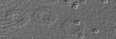
Flatfield frames are obtained during photometric runs to remove mainly pixel-to-pixel sensitivity variations and (typically two-sized) defocused images of dust grains sitting on the filter wheel and on the CCD. Usually, when the telescope is not defocused (see e.g., Kjeldsen & Frandsen, 1992; Southworth et al., 2009) or when it is not guiding, once science frames are bias-subtracted and flatfielded, small imperfections can be observed. This can be acknowledged by visually inspecting the calibrated science frames, and sometimes by observing that the red noise in the light curves is correlated with the centroid position of the stars, which might change in time due to drifts on the detector caused from imperfect tracking and/or seeing variations. This residual variability is mostly caused by the finite precision that the flat fields have to reproduce the imperfections on the CCD. In this work we have simulated flats reproducing some features that can be usually observed in such frames: pixel-to-pixel variability, central excess illumination, cosmetics caused during the construction of the CCD, and shadows of dust grains, which can take two different sizes depending on if they are located directly over the CCD (small size) or over the filters (large size). Since most of these parameters depend on the CCD quality, the values that the flat field take in our simulations depend on the selected observatory. We have also added an effect that is caused by Moonlight, thus correlated with the Moon phase: when skyflats or domeflats are obtained, the illumination is expected to be homogeneous. However, when observations are carried out under Moonlight, the shadow of the dust grains is projected in a slightly different direction, depending on where the Moon is in the sky relative to the target star during the observations. Therefore, when flat fields are used to correct science frames obtained during gray/bright nights, bright and dark spots can be observed sometimes even by eye in the location of the dust grains. This effect, along with the synthetic flat fields produced in this work, can be observed in Figure 1.

Figure 1: Fraction of simulated flat fields. Top, left: two sized dust grains, pixel-to-pixel sensitivity variability and uneven illumination can be observed. Top, right: as comparison, a real flat frame. The pixel and gray scales are different. Bottom: how a science frame would look like when taken during Moon light. The dark and bright spots can be easily observed.

In this work we include the flat field residual modulation as follows: the code randomly chooses two positions over the synthetic flat field representing the positions of the target and one reference star. The distance between both is chosen randomly. Then, their positions are drifted over the image, creating an (x,y)($t$) array whose length is equal to the length of a given observation. Depending of the telescope in question, the amplitude of the drift is going to be larger (OAM, assuming no guiding system) or smaller (HSO and MCD, assuming some sort of guiding). Also, we consider the (x,y) drift to be more prominent in one direction, assuming that the telescope is drifting more in right ascention, as it is normally the case with real telescopes. The quality of the flat (the pixel-to-pixel variability) also depends on the telescope. We assumed that the larger the telescope, the more expensive the CCD is and, therefore, the more accurate the flat is. We then integrate flat counts inside an aperture that corresponds to an integration area of 40 pixels², and divide the count rate of the target by the count rate of the reference star in each time stamp. Finally, we normalize and scale the amplitude of the modulation down to a random number between 2 and 10 parts-per-thousand, to meet typical amplitudes of instrumental modulation. The computed variability is then saved, along with the (x,y) position, to be used during the detrending instance.

3.3 Residual modulation due to first order atmospheric extinction

First order atmospheric extinction, (i.e., extinction independent of stellar color), is airmass dependent. Since differential photometry involves at least two stars at different elevations, a residual modulation due to airmass differences can be detected, increasing when the elevation difference between the target star (sub-index $\star$) and the reference stars (sub-index $1,2,\cdots,n$) increases as well. For any star, absorption by the atmosphere can be described by Bouguer’s law:

$$m=m_{0}-\kappa\chi\;,$$ (10)

where $m_{0}$ denotes the stellar magnitude outside the atmosphere, $\kappa$ the extinction coefficient in magnitudes per airmass (mag/AM), $\chi=\sec(z)$ the airmass value during a certain observation, and $z$ the zenithal distance of the star. Since light curves are produced only when the altitude of the star at mid-transit time is larger than 35^∘, the linear representation of airmass is sufficiently accurate.

To decrease the scatter of the final light curve, it is of common practice to consider as reference star the combination of many others. Hence, considering Bouguer’s and Pogson’s laws, the airmass modulation, $AM_{\mathrm{mod}}$, that will affect the differential light curve will follow:

$$\log(AM_{\mathrm{mod}})=\frac{\kappa}{2.5}\left(\chi_{\star}-\frac{1}{n}\sum_{i=1}^{n}\chi_{i}\right)\;.$$ (11)

The second term between the parentheses accounts for the combined airmass contribution of $n$ reference stars.

The top panel of Figure 2 shows how the airmass difference between target and one particular reference star evolves, as a function of the angular separation between stellar objects (color-coded) and the hour angle, $t$, where $t=0$ denotes the culmination of the target star. The bottom panel of the same Figure shows how the airmass modulation $AM_{\mathrm{mod}}$ evolves, as the stars move across the sky. Note that the angular separation between stars is constrained by the size of the field of view of each telescope.

Figure 2: Top: airmass difference between target and reference star, as a function of hour angle, in units of $10^{-3}$. Bottom: airmass modulation due to airmass differences (Eq. 11), in units of $10^{-4}$. The lines correspond to an angular separation of 7 arcmin and $\kappa_{HSO}$ = 0.2 mag/AM (gray), 15 arcmin and $\kappa_{MCD}$ = 0.14 mag/AM (pink) and 20 arcmin and $\kappa_{OAM}$ = 0.18 mag/AM (cyan).

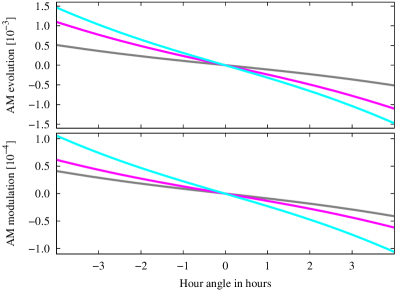
To calculate the airmass, $\chi_{i}$, for each reference star, we use the previously selected $\Delta\alpha$ and $\Delta\delta$ displacements, relative to the target star. Although the modulation effect is small, it rapidly increases with the angular separation between target and reference stars. Since small telescopes tend to have large fields of view ($\sim 1$ deg or larger) we consider this effect relevant and the first atmospheric-correlated noise source. The unaffected transit light curve is deformed by $AM_{\mathrm{mod}}$.

3.4 Color-dependent residual modulation

Extinction is caused by absorption and scattering of light. Water vapor, ozone, and dust, but mostly Rayleigh scattering in the optical, are contributing to it. Color-dependent extinction (or “second-order extinction”) appears because the light of a stellar object, on its path through the atmosphere, has a wavelength-dependent absorption. In consequence, if two stars of dissimilar intrinsic color indexes are observed at the same altitude, their respective absorption will differ.

When the differential photometry technique is performed using stars of different spectral types, a color-dependent residual shows up. Frequently, the spectral information of the stars involved in the differential photometry is completely missing. Therefore, the effect can not be modeled out. To model it in, we followed Broeg et al. (2005) methodology (see their Section 4.2 for a complete analytic description). For each observation instant $j$, the second order extinction modulation $SOE_{\mathrm{Mod}}$ follows:

$$SOE_{\mathrm{Mod}}=R(T_{\star},\chi_{\star,j})/(\Pi_{i=1}^{n}\ R(T_{i},\chi_{i,j}))^{1/n}\;,$$ (12)

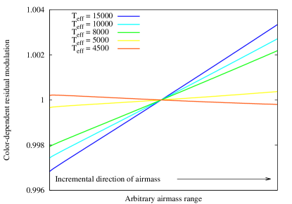
where $R(T_{\star},\chi_{\star,j})$ accounts for the flux change of the target star due to the Earth’s atmosphere, while $R(T_{i},\chi_{i,j})$ does so for each one of the reference stars $i=1,\ldots,n$. The wavelength dependency has been already integrated out. It involves the filter transmission function, the quantum efficiency of the CCD, and the black-body curves of the target and reference stars. Figure 3 shows how the second order extinction amplitude depends on the spectral type of the chosen reference stars. Considering a target star with $T_{\mathrm{eff}}$ = 4 900 K (similar to Qatar-1), we estimated the strength of $SOE_{\mathrm{Mod}}$ for one given reference star with effective temperatures 3 000, 4 500, 5 000, 8 000, 10 000, and 15 000 K. As the Figure clearly reveals, the effect grows when the difference between spectral types maximizes. Note that the slope of the residual modulation changes from positive to negative, when the effective temperature of the reference star turns from being larger to smaller than the effective temperature of the target star.

Figure 3: Color-dependent residual modulation considering different effective temperatures for the reference stars.

3.5 Scintillation

Astronomical seeing refers to the blurring of astronomical images caused by the turbulence in the Earth’s atmosphere. In addition, the brightness of stars appears to vary due to scintillation, which is caused by small-scale fluctuations in the air density as a result of temperature gradients. Based on Young (1993)’s approach, we estimate the contribution of scintillation noise to the accuracy of photometric measurements:

$$S=0.0030\ D^{-2/3}\ \chi^{3/2}\ e^{-h_{\mathrm{obs}}/h_{0}}\ \tau^{-1/2}\;,$$ (13)

where $D$ is the telescope diameter in meters, $h_{\mathrm{obs}}$ is the altitude of the observatory above sea level in km for $h_{0}$ = 8 km, and $\tau$ the exposure time in minutes. In differential light curves scintillation translates directly into the scatter of the data. To include this effect into our light curves, we calculate random Gaussian noise with $\mu=1$ and $\sigma$ equal to the given scintillation semi-amplitude. The only changing factor on Young’s scintillation expression is the airmass, so the standard deviation will not be constant but will be modulated by the star’s altitude, as seen in real light curves, where photometric precision decreases with $\chi$ for a fixed exposure time. Consequently, the primary transit synthetic light curves account for scintillation as well.

3.6 Non-photometric conditions

3.6.1 Irregularities caused by changes in the atmospheric seeing

Although large telescopes are located in the most convenient sites with respect to altitude and photometric conditions, this is not always the case for decimeter–to–meter class telescopes. Small telescopes are located all over the world, where photometric conditions can be far from optimal. Abrupt changes in the atmospheric transparency, the humidity and the ambient temperature, added to cirrus and clouds passing by, can produce unwanted photometric variability. In such sites, atmospheric seeing tends to quickly degrade with airmass.

Aperture photometry involves the measurement of stellar fluxes within a fixed aperture radius. Thus, during any data reduction process the aperture radius can be selected to coincide with, for example, the full-width at half-maximum (FWHM) of the first image. For instance, if the observations are carried out only after culmination, as a product of the degradation of the atmospheric seeing the integrated flux inside the fixed aperture will decrease with time. If changes in the photometric conditions would propagate equally to all the stars within the field of view, the differential photometry technique would be satisfactory to remove correlated noise produced by those changes, although the amount of white noise would still change as a function of time, since the number of photons collected in each aperture would change as the stars cross the sky. Nonetheless, real photometry reveals that the point spread function (PSF) of all the stars slightly differ from one another. Therefore, differential light curves will show a residual modulation strongly correlated with airmass. To model this effect, we made use of physically and empirically motivated relationships.

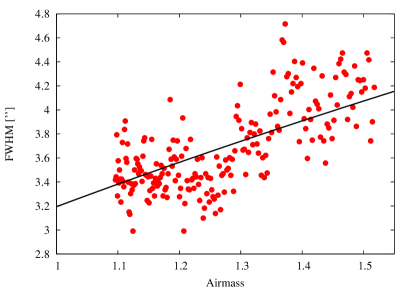
Although atmospheric seeing is a very local measurement that strongly depends on the position of the turbulent atmospheric layers, we started considering seeing as scaling with the airmass to the power of 0.6 (see e.g., Sarazin & Roddier, 1990; Gusev & Artamonov, 2011). Figure 4 shows the evolution of seeing (equivalently, FWHM) as a function of airmass. The FWHM measurements correspond to Qatar-1, from observations carried out at Hamburger Sternwarte. The black continuous line indicates a fit to the data of the form $FWHM(\chi)\propto\chi^{0.6}$. As it can be seen, the relation properly reproduces the FWHM general trend. During the observations the telescope was slightly defocused. Therefore, the values of the FWHM are not a realistic measurement of the characteristic seeing of the site.

Figure 4: FWHM evolution as a function of the airmass. Red points show true measurements of FWHM (arcsec), while black continuous line indicates the $FWHM(\chi)\propto\chi^{0.6}$ dependency.

Furthermore, the stellar integrated fluxes are estimated as the area within a two-dimensional normal function, $G(\mu,\sigma)$. The FWHM is related to the normal function via the standard deviation, $\sigma$, as $FWHM=2\sqrt{2\ln(2)}\leavevmode\nobreak\ \sigma$. For a given aperture radius $R_{\mathrm{ap}}$ and FWHM, the area is easy to integrate. In polar coordinates, for any given star:

$$F_{\star} = \int_{0}^{2\pi}\int_{0}^{R_{ap}}G(r,\theta)\leavevmode\nobreak\ r\leavevmode\nobreak\ dr\leavevmode\nobreak\ d\theta$$ (14)

$$= \int_{0}^{2\pi}\int_{0}^{R_{ap}}A\ e^{-r^{2}/2\sigma^{2}}\leavevmode\nobreak\ r\leavevmode\nobreak\ dr\leavevmode\nobreak\ d\theta\;,$$

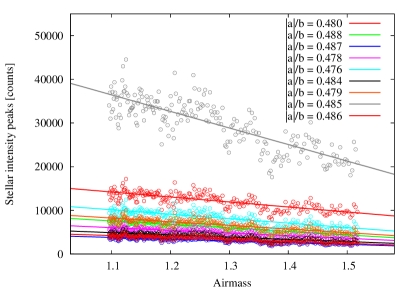
where $A$ denotes the intensity peak of the normal function. For a fixed exposure time, an increase in airmass translates into a decrease in the intensity peak. To shape this out, we studied the intensity peak evolution present in our observations of Qatar-1. Figure 5 shows the evolution of $A$ as a function of airmass, for $n=9$ stars. From our combined HSO and OAM data we found that a linear relation, in the form:

$$A(\chi)_{i}=-a_{i}\chi+b_{i}\;,a>0\;,$$ (15)

is sufficient to properly reproduce the observed variation. Furthermore, the relation between the slope and the intercept satisfies:

$$|a_{i}|/b_{i}=\mathbb{C}+\epsilon_{i}\;,$$ (16)

for each star $i$ within the field of view, for $\epsilon\ll 0$, and $\mathbb{C}$ a number close to 0.5. Independently of the intrinsic brightness of the stars, our observations reveal that the ratio $|a_{i}|/b_{i}$ remains approximately the same during a given observing run, as reflected in Eq. 16.

Figure 5: Intensity peaks of 9 stars within the field of view of HSO, as a function of airmass (saturation level of HSO CCD lies at 65535 counts). Linear trends, as reported in Eq. 15, are over-plotted in continuous lines.

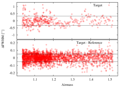
With the FWHM and $A$ empirically described as a function of airmass, we re-analyzed our observations to set constraints on the dispersion of both parameters. As an example, the top panel of Figure 6 shows the variation of the FWHM for Qatar-1 with respect to the mean FWHM of the night. In the bottom panel of the Figure we show the relative difference between the FWHM of Qatar-1 and the FWHM of eight reference stars within the field of view of HSO. We used two times the standard deviation of the data points as an upper limit to assess the dispersion of the FWHM. Equivalently, a similar procedure was repeated for the intensity peaks.

Figure 6: Changes in the FWHM for Qatar-1 (top) and for eight reference stars (bottom) relative to Qatar-1. Airmass values between 1 and 1.2 are over-sampled with respect to the rest, because the star was observed before and after culmination. The standard distribution of both data sets was used to set constraints on the scatter of the simulated FWHM.

To model the residual modulation in the light curves caused by changes in the photometric conditions, for each epoch the code generates the random number $\mathbb{C}$, close to 0.5. Then, for the target and the $i=1,\ldots,n$ reference stars, the code produces $n+1$ values of $\epsilon_{i}$ and $n+1$ values of $a_{i}$. With Eq. 16 the intercepts $b_{i}$ are determined, and by means of Eq. 15 the peak intensities for the $n+1$ stars are finally obtained. The resultant modulation is given by:

$$FWHM_{\mathrm{mod}}=F_{\star}/(\Pi_{i=1}^{n}F_{\mathrm{ref},i})^{1/n}\;,$$ (17)

The primary transit light curves are then modified by the estimated $FWHM_{\mathrm{mod}}$.

3.6.2 Effects associated to poor observing conditions

A photometric night is neither defined by the brightness of the sky, nor by its extinction value. Since an increase of the sky brightness can be compensated by longer exposure times, and a low extinction coefficient only means that the sky is fairly transparent, what defines a photometric night is the stability of the sky conditions as the night evolves. Obviously, not all nights are photometric. Cirrus cloud formation (i.e. thin clouds holding ice crystals located at altitudes above 5000 m) are a common phenomenon. They can be easily noticed during the day or during the night under the presence of the Moon, when Moonlight is reflected by the ice crystals within the clouds. However, cirrus can go unnoticed during dark nights.

When sky conditions are far from optimal, true flux levels of stellar sources cannot be properly measured. They are modulated by the continuous fluctuations dominating the sky conditions. Generally, sky variability translate into the data in two forms. In the first case, the scatter of the data are correlated with the night quality. In the second case, when the clouds are inhomogeneous throughout the field of view and change their position rapidly, the light curves show data points clearly outside the normal data distribution. In addition, observatories can be light-polluted. This dramatically reduces the visibility of the stars and enhances, in turn, the effects associated to fluctuations of the night sky.

Due to the random nature of this effect, we approach its modeling by analyzing real HSO and OAM Qatar-1 data. To this end, we considered 23 observing nights and counted how many points were observed away from the normal distribution. A given photometric point was considered an outlier if it was more than $\pm 2\sigma$ displaced, being $\sigma$ the natural scatter of the data, estimated from each residual light curve. From the analyzed HSO and OAM light curves of Qatar-1, among a total of 2651 data points, 136 were outside the $\pm 2\sigma$ limit, which corresponds to 5.13% of the total datapoints. Therefore, for each synthetic light curve the code randomly selects between 3% to 7% of synthetic data points to be placed as outliers. To produce the shift, we calculated a local standard deviation, taking into account only the flux measurements in the vicinity of the randomly selected points, in order to correlate the amplitude of the jump with the actual local dispersion of the data. We then randomly increase or decrease the position of the points from two up to three times the local standard deviation. Their corresponding error bars are increased by the same amount. We don’t consider increasing the jump further, because it is of common use to filter outliers above $\pm 3\sigma$ (see e.g., Moutou et al., 2004).

3.7 Photometric errors

Photometric errors are usually provided by a photometric reduction task. However, reduction tasks do not account for systematic effects over the photometry. As a consequence, the photometric errors are slightly underestimated (see e.g., Gopal-Krishna et al., 1995, for IRAF’s case). For this reason, we did not use the magnitudes of the errors of real photometric data to create the synthetic ones, but analyzed them to quantify their dependence with airmass and the frequency at which they vary. From real error measurements we found that a linear correspondence with airmass can properly represent how do error magnitudes change as the stars cross the sky. Furthermore, due to continuous changes in the sky conditions the photometric errors also fluctuate. To estimate the frequencies, $\nu_{k}$, at which the sky tends to vary more often, we run a Lomb-Scargle periodogram (Lomb, 1976; Scargle, 1982; Zechmeister & Kürster, 2009) over the errors computed with IRAF’s phot task over OAM and HSO data. To this end, we analyzed 25 observing nights at HSO spanning two years, and 10 nights at OAM covering one year. Once individual periodograms were calculated, we added them up and used the four main peaks that are more relevant for a transit observation duration (of the order of a couple of hours) to describe the fluctuations of the sky (Figure 7).

Figure 7: From top to bottom: most representative sky fluctuations for OAM (cyan line) and HSO (pink line). The bottom plot corresponds to the errors for one observing night at HSO. In black, considering the four main frequencies, $\mu$ and $\sigma$, we fitted only the phases to the light curve (black line) to show the goodness of our approach.

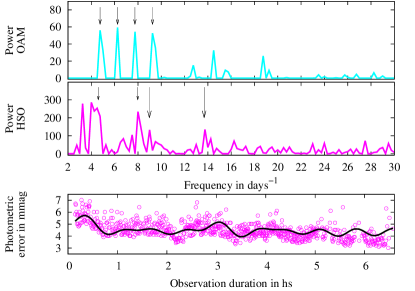
For our synthetic data as error magnitude, $\epsilon$, we used the standard deviation of the residual light curve once the stellar intrinsic and instrumental variability were added to the light curves (see Sections 3.2 to 3.7). Using $\epsilon$, the frequencies $\nu_{k}$ at which the sky tends to vary more often, and a phase value $\phi_{k}$ randomly selected between 0 and 1, the final photometric errors $\hat{\epsilon_{j}}$, for each observation $j$, are estimated as follows:

$$\hat{\epsilon_{j}}=\epsilon_{j}\prod_{k=1}^{m}\ \sin\ [2\pi(\nu_{k}\ BJD_{j}+\phi_{k})]\;,$$ (18)

with m = 1,$\cdots$,4.

3.8 Final light curves

Figure 8 shows how one particular synthetic light curve evolves, when the correlated noise sources are sequentially added to it. From top to bottom we show the Mandel & Agol (2002) transit model (a), the latter when the instrumental and environmental effects are being added to the transit model (b), how scintillation reflects into the light curve (c), and how non-photometric conditions impact the data (d). In this case, the error bars have been scaled so that their averaged value can meet the standard deviation of the data. The final light curve, with its photometric errors enlarged by its corresponding $\beta$ value (see Section 4.1), can be found under (e). These are the primary transit light curves from which the mid-transit times will be retrieved.

Figure 8: From top to bottom: (a) Initial transit light curve (Sect. 2.2). It defines the duration of the observation. From now on, all the previous effects are considered in the next light curve. (b) Instrumental (Sect. 3.2) and atmospheric (Sect. 3.3, Sect. 3.4) inhomogeneities. (c) Scintillation (Sect. 3.5). (d) Effects related to poor observing conditions and seeing-related variability (Sect. 3.6, Sect. 3.6.1, and Sect. 3.6.2) plus photometric errors (Sect. 3.7). The average value of the error bars has been scaled up to meet the standard deviation of the light curve. (e) Same as (d), but the error bars have been enlarged by $\beta$ (Sect. 4.1). The next quantities have been scaled and shifted to meet the plot. AM: airmass trend during observations. PE: time-variability of the photometric errors. FC: integrated counts in the synthetic flat field following the computed (x,y) pixel shifts.

4 Testing our light curves: Real vs. synthetic data

Figure 9 shows real versus synthetic transits of Qatar-1. In both cases, the observations were performed and simulated using Johnson-Cousins R filter and Oskar Lühning Telescope at HSO.

Figure 9: Real (red) and synthetic (green) light curves of Qatar-1, produced using Oskar Lühning telescope and Johnson-Cousins R filter. Bottom panel shows how error bars change due to non-photometric conditions.

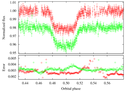
As initial test, both light curves are visually comparable. The most important difference (and advantage) in favor of synthetic light curves is the fact that correlated noise sources are completely known. For real light curves, however, one can only estimate how much are they affected by red noise, but not exactly why and how. In order to properly test the similitude between real and synthetic light curves, we performed a more concise analysis described in detail under the following Sections.

4.1 Comparing time-correlated noise structure

Pont et al. (2006); Carter & Winn (2009) and references therein investigated how time-correlated noise affects the estimation of the orbital parameters. To quantify how dominated are our synthetic light curves by red noise, we reproduced their analysis as follows: by subtracting the primary transit model to each light curve, we produced light curve residuals. We then produced M equally-large bins, varying M between 1 and 40 depending on the available data points per transit light curve and calculated N, the average value of data points per bin, which accounts for unevenly spaced data. If residuals are not affected by red noise, they should follow the expectation of independent random numbers (Winn et al., 2008):

$$\sigma_{N}=\sigma_{1}N^{-1/2}[M/(M-1)]^{1/2}\;,$$ (19)

where $\sigma_{1}$ is the sample variance of the unbinned data. $\tilde{\sigma_{N}}$ is the standard deviation of the binned data:

$$\tilde{\sigma_{N}}=\sqrt{\frac{1}{M}\sum_{i=1}^{M}(\mu-\mu_{i})^{2}}\;,$$ (20)

where $\mu_{i}$ corresponds to the mean value of the residuals inside each bin, and $\mu$ to the mean value of the means $\mu_{i}$. If correlated noise is present, then each $\tilde{\sigma_{N}}$ will differ by a factor $\beta_{N}$ from their expectation $\sigma_{N}$. By averaging $\beta_{N}$ over timescales that are judged to be important for transit observations (ingress or egress duration), the parameter $\beta$ can be estimated. $\beta$ accounts for the strength of correlated noise in the data. For Qatar-1, the time between first and second contact (or equivalently, the time between third and fourth contact) is $\Delta n\sim$ 15 min. To estimate $\beta$, we averaged individual $\beta_{N}$’s calculated out from bins with sizes 0.8, 0.9, 1.0, 1.1 and 1.2 times $\Delta n$.

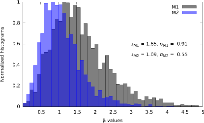
Figure 10 shows two normalized histograms of the $\beta$ values that were computed from the available synthetic light curves produced after 2$\times$35 runs of our code. In more detail, the $\beta$’s were calculated from the residual synthetic light curves, which in turn were obtained fitting to the synthetic data a transit model in simultaneous to a time-dependent low-order polynomial (M1, black), and a transit model in simultaneous to a linear combination of some time-dependent environmental and instrumental quantities such as airmass, seeing, and integrated flat counts (M2, blue). For a more detailed description about the normalization process, we refer the reader to Section 5. Generally, $\beta$ = 1 corresponds to data sets free of correlated noise. $\beta$ values smaller than 1 are due to statistical fluctuations and are neglected in this work. In other words, if a $\beta$ value turns out to be smaller than 1, the error bars are left unchanged. The most representative values of the histograms and their scatter, ($\mu$, $\sigma$), are added to the plot. As the histograms reveal, M2 data detrending appears to take care more properly of systematics in the data, since their retrieved $\beta$’s appear to cluster closer to 1.

Figure 10: Histogram of the strength of correlated noise $\beta$ considering raw (blue) and normalized (black) synthetic light curves.

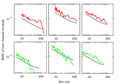
To test the $\beta$-values obtained from our synthetic data, we compared them to $\beta$-values obtained from real photometry. For a quick comparison of the noise structure, Figure 11 shows the results of our correlated noise analysis for the longest three nights of Qatar-1 real data on top (red lines), and three synthetic light curves with similar duration and cadence on bottom (green lines). In all cases, black lines show how residuals should behave in absence of red noise. Red and green lines represent the variance of the binned data for HSO real and synthetic light curves, respectively, as a function of the bin size. As expected, the larger the bin size, the smaller the RMS. For some of our available Qatar-1 primary transit light curves we estimated $\beta$ by averaging $\beta_{N}$ over the same 5 bin sizes already stated. Comparing the synthetic $\beta$-value distributions against the ones obtained from real data, $\sim$90% of our synthetic light curves present the same amount of correlated noise. Considering that the number of synthetic light curves significantly exceeds our observations, the correlated noise is indeed comparable.

Figure 11: RMS of time-binned residuals as a function of bin size for real (red and top) and synthetic, M1-normalized (green and bottom) light curves.

4.2 Comparing autocorrelation signals

In statistics, autocorrelation occurs when residual error terms from observations of the same variable at different times are correlated. If residuals are dominated by Gaussian white noise, then the normalized autocorrelation of the residuals follows a normal distribution with mean $\mu$ = 0 and dispersion $\sigma$ = 1/N, being N the number of data points. Ideally, for white noise most of the residual autocorrelation signal should fall within 95% confidence bands around the mean. If the autocorrelation signal of a given data set doesn’t behave as mentioned, then the data accounts for correlated noise.

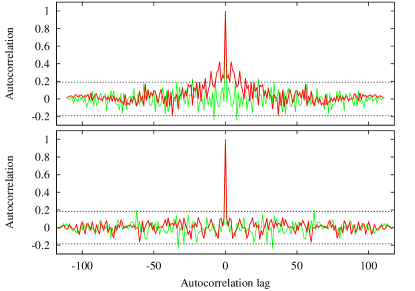
Figure 12 shows an example of the difference in the residual autocorrelation that exists among real photometry of Qatar-1 obtained during two different nights. As a comparison, the autocorrelation for simulated residuals affected only by Gaussian white noise is plotted in green, along with the 95% confidence band indicated in black-dashed lines. The autocorrelation function for two HSO observing nights is plotted in red. On top, the real light curve is affected by correlated noise, since the central part of the autocorrelation function clearly escapes the 95% confidence band. On bottom, correlated noise appears to be negligible.

Figure 12: Autocorrelation function for real residual light curves (red) and simulated white noise (green) as comparison. The 95% confidence band is indicated with black-dashed horizontal lines. Top: real data with correlated noise. Bottom: Autocorrelation function falls inside the 95% confidence band.

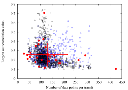
Furthermore, we compared the autocorrelation structure between real and synthetic data sets (Figure 13). The autocorrelation function was calculated from the residual light curves, obtained after the primary transit model was subtracted. To compare real to synthetic light curves we carried out the following analysis: we first calculated the autocorrelation function of real photometric data, and plotted the largest autocorrelation value $AC_{max,real}$ as a function of the data point number (red filled circles). Since it only takes to validate $AC_{max,real}$ against the 95% confidence band to estimate if the light curves are indeed affected by red noise, we considered sufficient to use $AC_{max,real}$ to compare both sets. As expected, there is a trend that follows smaller $AC_{max,real}$ values for larger N’s. Finally, we estimated $\mu_{AC_{max,real}}\pm\sigma_{AC_{max,real}}$ and $\mu_{N}\pm\sigma_{N}$.

We then repeated the same process calculating the largest autocorrelation value from residuals obtained subtracting to the synthetic light curves the transit model only (blue) and a transit model times a second order time-dependent polynomial (black). In both cases, $\sim$80% of the data points fall within the 1$\sigma_{AC_{max,real}}$, plotted in Fig. 13 with red error bars. Taking into account that we count with substantially more synthetic than real data, the remaining 20% can be neglected. Therefore, real and synthetic data seem to present similar correlated noise structure.

Figure 13: Largest autocorrelation value (LAC) for synthetic data calculated from residuals obtained subtracting to the synthetic light curves the transit model only (blue) and a transit model times a second order time-dependent polynomial (black). Over-plotted in red, the LACs for 25 real observations that were obtained using HSO and Johnson-Cousins R filter.

4.3 Comparison with previous works

A way to study the impact of systematics over the determination of the mid-transit times is to produce systematic components with similar time-scales as the instrumental and environmental systematics, and to generate synthetic light curves by adding stochastic functions with similar amplitude and frequency to the real noise present in photometric data. This approach has been already carried out by other authors. For example, Carter & Winn (2009) created synthetic light curves which correlated noise was represented by the sum of two uncorrelated and correlated Gaussian processes, and focused on the impact of this noise structure over the determination of the mid-transit times. Gibson et al. (2013) created synthetic data adding up a “function noise” that was build by summing up 100 exponential, Gaussian, and sinusoidal functions with random parameters, with the main goal to test the accuracy of the retrieved orbital parameters. Although the analysis we have in common produce results that do not differ (see Section 5) the main differences between our method and previous work is that, in our case, the time dependency is represented more realistically. For example, our method accounts for noise that improves or degrades as the stars cross the sky (airmass and seeing dependency), which is observed in real photometric data. We can also investigate the impact of current detrending techniques into the determination of the orbital and physical parameters of the system (see Section 6), because we have environmental and instrumental quantities (e.g., airmass, seeing, and changes of the centroid position of the star over the CCD) that can be used to understand the impact of these systematics over transit light curves. Indeed, in this work we study how much does the precision of the orbital and physical parameters improve when a certain normalization is being considered, which would have been impossible to carry out when only stochastic functions are used to represent the noise.

5 Recovering the TTV signal: General aspects

Once the synthetic light curves are generated (usually between 50 to 70 each run), recovering the TTV signal is the next step to follow. Before transit fitting begins, we visually inspect the generated light curves, removing those presenting extremely poor transit coverage, scatter larger than the transit depth, and highly affected by correlated noise. The number of deleted light curves clusters around 5-10 per run. Then, the TTV recovery goes as follows:

• To obtain good estimates for the system parameters, we select the five best light curves according to the following criteria: they should have a good amount of OOT data before and after transit begins and ends, respectively, small scatter compared to the transit depth, and good cadence. The transits should also be well spread along the 400 epochs to retrieve an accurate orbital period, and should be divided among the 5 filters and the 3 observatories that the code considers (Sect. 2.3). It is worth to mention that an incorrect selection of transit light curves (i.e., by considering primary transits with large scatter, incomplete, or strongly affected by correlated noise) leads to very inaccurate orbital parameters. This selection was done by visually inspecting the light curves generated over more than 60 full runs of the code.

• From the latter sub-sample, we choose the best light curve with respect to data scatter and sampling rate. It will be considered as the 0^th epoch.

• Together with the transit model (Mandel & Agol, 2002) we simultaneously fit to the data two models accounting for the non-transit variability, but separately. In other words, for each run we will fit the data twice. To reproduce as best as possible current data detrending techniques, in this work we consider a low-order time-dependent polynomial (first, second or third order, from now on called M1 normalization). The selection of the order is carried out light curve by light curve by minimizing the Bayesian Information Criterion, BIC = $\chi^{2}$ + k ln(N). For the BIC, k is the number of fitting parameters, N is the number of data points per light curve, and $\chi^{2}$ is computed from the residuals, which in turn are obtained by subtracting to the synthetic data the best-fit model with its corresponding time-dependent polynomial. As detrending function we also consider a linear combination of airmass (AM), seeing (SN), x and y pixel position ($x_{pix},y_{pix}$) and integrated flat counts in those (x,y) values (FC), from now on called M2 normalization. All these quantities are provided by the code. Thus, in the first case the detrending fitting parameters are up to four, while in the second case they are six: the previously mentioned ones plus an offset. In short, the time dependency of the normalization functions and the fitting parameters look as follows:

  $$M1(t)=a_{3}t^{3}+a_{2}t^{2}+a_{1}t+a_{0}\;,$$ (21)

  $$M2(t)=c_{0}+c_{1}\mathrm{AM}+c_{2}\mathrm{SN}+c_{3}x_{\mathrm{pix}}+c_{4}y_{\mathrm{pix}}+c_{5}\mathrm{FC}\;.$$ (22)

  The simultaneous fitting of the transit model and the detrending function is carried out in the same fashion not only to compute the orbital parameters of the system but to obtain the mid-transit times of the individual light curves.

• We then proceed to fit the five selected transit light curves by sampling from the posterior probability distribution using a Markov-chain Monte Carlo (MCMC) approach. From the transit light curve we can directly infer the following parameters: the orbital period, $P$, the mid-transit time, $T_{o}$, the planet to star radius ratio, $p=R_{p}/R_{s}$, the semi-major axis in stellar radii, $a/R_{s}$, the orbital inclination, $i$, and the limb-darkening coefficients. For our fits we assume a quadratic limb-darkening prescription with fixed $u_{1}$ and $u_{2}$ (Table 3). From now on, these are called global parameters.

• After $5\times 10^{5}$ iterations we discard a suitable burn-in ($10^{5}$ samples) and compute the best fit parameters from their posterior distributions (mean and standard deviation as best-fit values and errors). The errors for the global parameters are derived from the 68 % highest probability density or credibility intervals (1 $\sigma$).

• Afterwards, we fit each light curve individually in an equivalent fashion as in the two previous steps. To consider the existing information in the determination of the individual mid-transit times, rather than fixing the orbital parameters to their best-fit values we specify Gaussian priors on $a/R_{s}$, $i$, and $p$. Since now the transit light curves are analyzed separately the orbital period, $P$, is left fixed to the global best-fit value. As previously mentioned, the model fitted to the data is the product between the transit model and M1 or M2. Before the individual light curves are fitted, we calculate the $\beta$ value as specified in Section 4.1 and we enlarge the individual photometric error bars by it. Finally, we obtain the best-fit mid-transit times, $T_{o,k}$, along with their error estimates that are drown from MCMC chains at 1$\sigma$ levels.

• To produce the synthetic O–C diagram, we consider the “Calculated” mid-transits as an integer multiple (epoch number) of the global orbital period. “Observed” mid-transits are the ones individually fitted in the previous step.

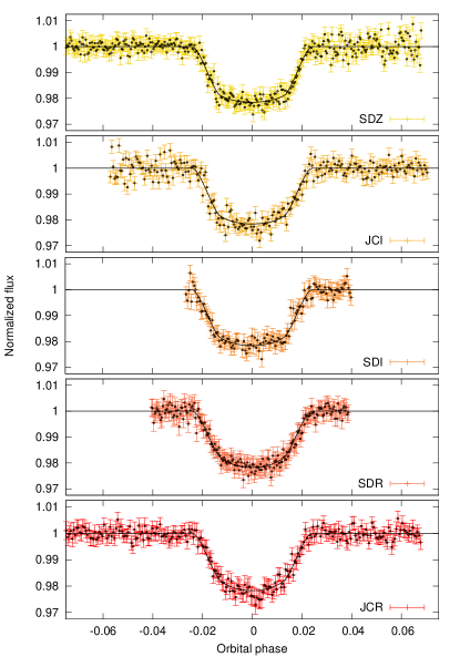
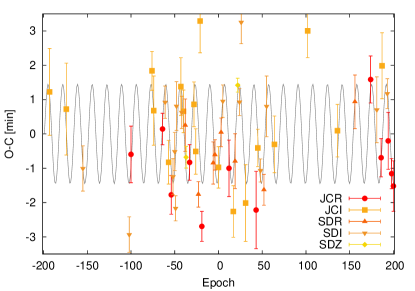
Figure 14 shows five synthetic light curves previously normalized by a time-dependent polynomial, one for each available filter. The data quality and their duration vary considerably. Light curves of this kind, combined all together, will be the ones used to perform the TTV analysis. In addition, Figure 15 shows one of the many synthetic O–C diagrams, obtained from the previously described procedure. The observed “grouping” of data points in the O–C diagram is caused by visibility effects, another feature observed in real transit follow-ups which can have an impact in the determination of the perturbers orbit if not treated properly (see Section 6.4).

Figure 14: Sample of synthetic light curves. In continuous line, Mandel & Agol (2002) primary transit model for each limb darkening coefficient set.

Figure 15: Synthetic O–C diagram. The mid-transit shifts are color-coded according to the randomly selected filter. The timing variation added by the code to each mid-transit time is plotted with gray continuous line. Clearly, some points scatter outside the true TTV signal.

6 Recovering the TTV signal: results

6.1 Determination of the global parameters for different normalization strategies

It is not news that the determination of the individual mid-transit times strongly depend on the normalization of the photometric data (Winn et al., 2008; Gibson et al., 2009), specially when incomplete light curves are taken into account. The choice of normalization has also an impact over the determination of the orbital and physical parameters, which in turn can affect the value of the mid-transit time. Therefore, we investigated the impact of the M1 and M2 normalizations by investigating the accuracy of the semi-major axis, the inclination, the orbital period, and the planet-to-star radius ratio.

The best-fit global parameters obtained as described in Section 5, along with their errors, are plotted in Figure 16. Black circles and 1$\sigma$ errors correspond to the global parameters obtained by means of synthetic data fitted against a transit model and M1. Blue squares and their respective 1$\sigma$ errors were obtained detrending the data using M2. The initial orbital parameters used by the code to produce the synthetic data are indicated in the plot by a red dot. The four plots in the lower part of the Figure reveal two obvious features: parameters obtained by M2 normalization have a significant less scatter than the ones obtained from M1. In consequence, they show more consistency with the values used as input, and full consistency when errors are at 2$\sigma$ level. The sub-plot from the upper-left part of Fig. 16 shows the already known correlation between the semi-major axis and the orbital inclination via the impact parameter $b=a\cos(i)$. Comparing both sets of solutions, these values reveal that not only the normalization has indeed an impact on the determination of the orbital and physical parameters, but the choice of normalization as well. Thus, the M2 normalization appears to better account for systematics and, in consequence, produces more accurate and consistent transit parameters.

Figure 16: Global parameters obtained normalizing the synthetic data via M1 (black circles) and M2 (blue squares). The red points indicate the values used by the code to produce the synthetic data, equivalently to the red vertical lines. The top three panels show the timing precision versus the derived transit parameters.

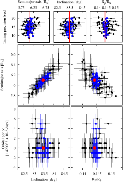
The three smaller panels on top of the Figure correspond to the timing precision (errors on the 0^th epoch at 1$\sigma$ level) versus the derived semi-major axis, $a$, the inclination, $i$, and the planet-to-star radius ratio, $R_{\mathrm{P}}/R_{\mathrm{S}}$. Although the mid-transit time (and in consequence its precision) should not depend on the physical transit parameters, it is not (always) the case, as observed in the Figure. When the M2 is used as detrending function there is no strong correlation between the timing precision and the precision of the transit parameters. However, when the data is detrended by a low-order time-dependent polynomial (M1) there is a strong correlation between the physical parameters and the timing precision. As the Figure shows, the uncertainties of the parameters increase as the timing precision decreases, as well as their scatter around the input value, creating in some cases inconsistency. It looks like the normalization procedure affects the transit parameters.

6.2 Significance of timing offsets: a more conservative approach

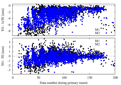
To estimate how much are the mid-transit times affected by the transit duration, we run the code 35 more times but shutting the TTVs off. Transits produced in this fashion were analyzed as described in previous Sections. Therefore, if any significant timing variability is present, this should be caused by systematics not properly taken care of. From these transits we computed the timing offset (TO) which is the absolute value of the difference between the observed timing shift and their expected shift (in this case 0), and subtracted to it their corresponding timing error, TE. A negative TO - TE would correspond to a TTV consistent with zero. Equivalently, a positive TO - TE would indicate a significant timing offset. The bottom panel of Figure 17 shows our results, when M1 and M2 normalizations are implemented (black circles and blue squares, respectively). TO - TE’s are plotted against the number of data points during primary transit, but the same exercise was performed for the number of OOT data points, the standard deviation of the residual light curves, and the transit coverage. The top panel of the Figure shows how an increment of the error bars to a 3$\sigma$ level gives timing offsets completely consistent with zero, an exercise that we would suggest the reader to carry out when assessing TTVs from ground-based observations. To quantify the correlation of the mid-transit times that would be consistent with TTVs (i.e., positive TO - TE) we used the Pearson correlation coefficient $r$:

$$r_{xy}=\frac{\sum_{i=1}^{n}\ (x_{i}-\mu_{x})(y_{i}-\mu_{i})}{[\sum_{i=1}^{n}\ (x_{i}-\mu_{x})^{2}\sum_{i=1}^{n}\ (y_{i}-\mu_{y})^{2}]^{1/2}}\;,$$ (23)

for $x$ number of data points during primary transit and $y$ the timing residuals. $r_{M1}=-0.25$ and $r_{M2}=-0.19$ confirm the existence of the correlation, which is observable even by visual inspection. Similar results were obtained analyzing the timing residuals against OOT data points and transit coverage. Thus, as previously observed by other authors we caution the use of incomplete light curves or poorly sampled primary transits to carry out TTV studies. This also reveals that TTVs derived from ground-based observations with amplitudes of the order of some minutes would be the consequence of either an improper treatment of the systematics, or an underestimation of the timing errors (Raetz et al., 2015) rather than caused by the interaction between two planets. Therefore, in this case we caution to make any statements about the detectability of TTVs.

Figure 17: Bottom: absolute value of the timing offset (TO) minus the timing error (TE) in minutes. Top: TO minus three times TE. Black circles correspond to M1 normalization and blue squares to M2. The plot has been produced from the analysis of 35 synthetic O–C diagrams.

6.3 Scatter in the O–C diagram: How much do systematics contribute?

When a periodogram analysis of the O–C diagram reveals a peak, it is of common practice to use the scatter in the O–C diagram to characterize the mass and orbital separation of a hypothetical perturbing planet (see e.g., Adams et al., 2010a, 2011; von Essen et al., 2013; Awiphan et al., 2016). To this end, different dynamical scenarios are considered and analyzed (for example, an inner perturber, an outer perturber, or two bodies in mean-motion resonances, Agol et al., 2005). In each dynamical configuration, the semi-major axis and the orbital eccentricity vary within a range of possible values. At each step, the scatter of the theoretical O–C diagram is computed, and compared to the observed one. This procedure is also repeated considering different masses for the perturbing body.

As seen in Section 6.2, poor primary transit coverage can yield to a considerably large timing offset that is completely independent of any TTV. Therefore, to understand whether unaccounted correlated noise sources lead to under- or over-estimations of the characteristics of the perturbing body, we analyzed again the scatter of the O–C diagrams for TTVs set on. In detail, we compared the scatter of the synthetic O–C diagram to the first order mean-motion resonance scenario. For each one of the normalization strategies we computed the observed standard deviation of each synthetic O–C diagram:

$$\sigma_{OC,synth}=\left[\frac{1}{N_{OC}-1}\sum_{k=1}^{N_{OC}}[T_{o,k}-(T_{o}+Pn_{orb,k})]^{2}\right]^{1/2}$$ (24)

where $N_{OC}$ is the number of light curves that the code generated in a given run, minus the ones that were deleted after visual inspection (Section 5). $n_{orb,k}$ corresponds to the orbit number with respect to the zeroth epoch, and $T_{o}$ and $P$ are the best-fit mid-transit time for the zeroth epoch and the orbital period, respectively. If two planets coexist in mean motion resonance, as pointed in Section 2.2 the perturbation term $PT(k)$ added to the unperturbed mid-transit times, for a given $k$ epoch, has the following expression:

$$PT(k)=\delta t_{max}\sin[2\pi P_{Trans}(k-1)/P_{lib}]\;.$$ (25)

From Eq. 25 we can compute the theoretically expected scatter:

$$\sigma_{model} = <(PT(k))^{2}>^{1/2}$$ (26)

$$= <(\delta t_{max}\sin[2\pi P_{Trans}(k-1)/P_{lib}])^{2}>^{1/2}$$

$$= (\frac{<\delta t_{max}^{2}>}{2})^{1/2}$$

$$= \frac{\delta t_{max}}{\sqrt{2}}\;.$$

Therefore, to estimate the perturbers mass by comparing the observed scatter, $\sigma_{OC,synth}$, to the theoretical one, $\sigma_{model}$, we require information about the orbital period and the mass of the transiting planet (which is normally known from transit photometry and radial velocity measurements), in addition to the order of the resonance. The only parameter that will vary, while comparing $\sigma_{model}$ to $\sigma_{OC,synth}$, is the mass of the perturbing body.

To calculate $\sigma_{model}$ we have to consider that each run provided slightly different orbital parameters (Section 6.1). Therefore, to be able to compare the results obtained at each run we considered the orbital period and the planetary mass used by the code as input parameters, and relatively large errors for the mentioned parameters (0.1% and 10%, respectively). Kipping (2010) studied the effects of finite integration times over the determination of the orbital parameters. If we consider the error on the mid-transit times that large exposure times produce, we will be able to define a lower limit on the amplitude of the TTV that we can realistically detect. Since we are considering only the case of first order mean-motion resonances produced by an Earth-sized planet, $j\geq 3$ would yield TTV amplitudes too small to be detected for exposure times of the order of one minute. Furthermore, j = 1 would produce TTV amplitudes easily to detect, even by means of these light curves (Agol et al., 2005). Therefore, it would not be inappropriate to restrict the resonance order to $j=2$, if our aim is to be consistent with the data that we have at hand.

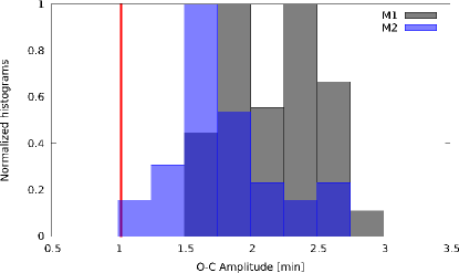
Figure 18 and Figure 19 summarize our results. The first Figure shows the derived amplitude of 35 synthetic O–C diagrams that were obtained implementing the M1 (black) and M2 (blue) normalization. While the black distribution has a mean value around 2.1 minutes, the blue one clusters around 1.5 minutes. The vertical red line indicates the amplitude in minutes that the input perturber causes. The second Figure shows the derived perturber masses assuming a j = 2 resonance. Propagating the errors of $P$ and $m_{Trans}$ previously mentioned allowed us to produce an error estimate for the perturbers mass. The latter is plotted horizontally and vertically in red.

Figure 18: Normalized histograms of the amplitude of the synthetic O–C diagrams when the M1 (black) and M2 (blue) normalizations are performed. The vertical red line shows the expected TTV amplitude produced by the perturber.

Figure 19: Retrieved mass of the perturber from the amplitude of the O–C diagrams in black circles for the M1 (x-axis) and M2 (y-axis) normalization. The black square with error bars shows the mean value and standard deviation of the points. In red horizontal and vertical lines, the expected mass of the perturber. The red area accounts for errors in the mass and orbital period of the transiting planet.

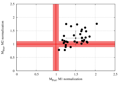
After comparing the predicted to the observed scatter, we found two main results: first, the scatter of the synthetic O–C diagram, associated to M1 and M2 normalization, seem to overestimate the action of the perturber. Although the M2 normalization appears to represent it more adequately, it is only consistent with it in few cases. We understand this as an improper treatment of the systematics. Second and most importantly (and consequent to the first case), the planetary masses obtained from the scatter of the synthetic O–C diagrams are over-estimated in most of the cases by around 50% in the case of M1 normalization and around 20% for the M2 normalization. Therefore, determining characteristics from the perturber using poor transit light curves will only provide miss-leading results about the system under study.

6.4 Periodogram analysis

In both continuous and discrete cases, Fourier theory explains how any function can be represented or approximated by sums of simple trigonometric and periodic functions. Given any time series, it is possible to find sines and cosines with different periodicity, phases and amplitudes that, when added together, can reproduce the time series back again.

Regarding TTV studies, once an O–C diagram is produced, the first natural step is to look for any kind of periodicity associated to the effects that a perturbing planet might cause on the timings of a transiting exoplanet. However, correlated noise sources affecting mid-transit times can disguise true signals. To test how much do systematic effects not properly accounted for affect the characterization of TTVs, we analyzed 35 O–C diagrams that were obtained from synthetic light curves not affected by transit timing variations, but affected by every systematic source instead. To this end we run a periodogram over each O–C diagram, searching for any leading frequency that could fake a planetary perturber signal but analyzing the M1/M2 scenarios separately. Once the frequency corresponding to the maximum power in the periodogram was found, we computed the spectral window of the O–C diagram to check that this peak was not caused by the sampling rate itself. To each one of the leading peaks we fitted a Gaussian function which mean and standard deviation correspond to the TTV libration frequency and its error. Values ranged between 10 and 200 days. For each peak we also computed the false alarm probability (FAP) (Horne & Baliunas, 1986) and also power values corresponding to FAP’s of 20%, 10% and 1%. Then, we counted how many times did these FAP’s exceeded the maximum power. From the 35 O–C diagrams, on average for the M1 and M2 scenarios, we found that the detected maximum peak was higher than FAP’s of 20%, 10% and 1% 14, 7 and 3 times, respectively. It is worth to mention that all these values should have been zero. Therefore, we caution the reader to give large FAP limits such as the ones provided here, when assessing significance levels on TTV periodicity. In our case, we had to decrease the FAP to 0.1% to have all the leading peaks below this level.

6.5 Quality factor

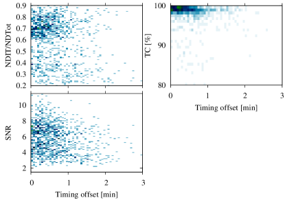
Rather than suggesting the reader to disregard TTVs obtained from poor light curves only, we attempt to characterize the quality of the light curves that, given 1$\sigma$ errors, were consistent with their expected timing value. In other words, these were light curves that, although they show a 1-2 minute offset from their expected value, they were still consistent within errors. This can be seen in Figure 20. The lower panel of the Figure shows a density map of the signal-to-noise ratio of the light curves, this is, the transit depth divided by the standard deviation of the residual light curves. The top left panel of the Figure shows the number of data points in transit (NDIT) divided by the total number of data points per transit light curve (NDTot). The right top panel of the Figure shows the transit coverage, TC, in percentage. 100% corresponds to light curves which primary transit was fully observed. The bluer the pixel in the density maps, the more light curves were showing these particular features. Thus, for example light curves with a SNR = 7, NDIT/NDTot = 0.7, and TC = 100% would provide reliable TTVs when the M2 normalization is performed. The three quantities characterized here can be easily obtained from transit photometry. Therefore, we suggest the reader to add this as quality check.

Figure 20: Density maps of light curves that produced consistent timings. From left to right and top to bottom the number of data points in transit (NDIT) divided by the total number of data points (NDTot), the transit coverage, TC, in percentage, and the signal-to-noise ratio of the light curve.

7 Discussion and conclusion

In this work we analyze whether current techniques used to detrend transit light curves taken from ground-based telescopes are suitable to properly characterize multiplicity in particular transiting systems via the transit timing variation technique. To this end, we simulated primary transit observations caused by a hot Jupiter which orbital and physical configuration mimics a real system, Qatar-1. To these light curves we artificially added a perturbation in their mid-transit times caused by an Earth-sized planet in a 3:2 mean motion resonance. The synthetic data accounts with what we believe are the most significant sources of light curve deformations: environmental variability (airmass, atmospheric extinction, and chaotic variability in the sky conditions during observations) and instrumental variability. We then tested the quality of our light curves, comparing their noise characteristics to the ones present in real data.

As already shown by other authors, our results disfavor the use of incomplete light curves to carry out TTV studies. Furthermore, our studies show that it is more likely that systematics not properly accounted for are causing the observed scatter in the O–C diagram rather than a gravitationally bound exoplanet. This, in consequence, produces mass estimates of the perturbing body that are a factor of up to two larger as expected. We also find that transits normalized by a time-dependent low-order polynomial provide more inaccurate and sometimes even inconsistent orbital and physical parameters than the ones derived from a more instrumentally and environmentally-related detrending function, which includes time-dependent variability such as changes of airmass, seeing, centroid position and integrated flat counts. Nonetheless, our results suggest that either both approaches are insufficient to account for systematics, or error estimates on the mid-transit times are being underestimated by current statistical techniques by a factor of up to three. A final inspection of the O–C diagrams and the light curves associated to each O–C point make us conclude that when only light curves with close-to-full transit coverage, good cadence, and large photometric quality are considered to carry out TTV studies, the derived O–C diagrams appear to be more consistent with their expected variability. In a future work we will investigate if the use of Gaussian Process regression can improve the determination of the perturbers characteristics, which would allow us to use low-quality transit photometry for TTV studies.

8 Acknowledgments

C. von Essen acknowledges funding by the DFG in the framework of RTG 1351, and E. Suarez and A. Ofir for fruitful discussions. Funding for the Stellar Astrophysics Centre is provided by The Danish National Research Foundation (Grant DNRF106). The authors acknowledge the referee for his/her positive feedback and suggestions to improve this manuscript.

References

- Adams et al. (2010a) Adams, E. R., López-Morales, M., Elliot, J. L., Seager, S., & Osip, D. J. 2010a, ApJ, 714, 13
- Adams et al. (2010b) Adams, E. R., López-Morales, M., Elliot, J. L., Seager, S., & Osip, D. J. 2010b, ApJ, 721, 1829
- Adams et al. (2011) Adams, E. R., López-Morales, M., Elliot, J. L., Seager, S., & Osip, D. J. 2011, ApJ, 728, 125
- Agol et al. (2005) Agol, E., Steffen, J., Sari, R., & Clarkson, W. 2005, MNRAS, 359, 567
- Alsubai et al. (2011) Alsubai, K. A., Parley, N. R., Bramich, D. M., et al. 2011, MNRAS, 417, 709
- Andersen & Korhonen (2015) Andersen, J. M. & Korhonen, H. 2015, MNRAS, 448, 3053
- Auvergne et al. (2009) Auvergne, M., Bodin, P., Boisnard, L., et al. 2009, A&A, 506, 411
- Awiphan et al. (2016) Awiphan, S., Kerins, E., Pichadee, S., et al. 2016, ArXiv e-prints
- Baglin et al. (2006) Baglin, A., Auvergne, M., Boisnard, L., et al. 2006, in COSPAR Meeting, Vol. 36, 36th COSPAR Scientific Assembly, 3749
- Ballard et al. (2011) Ballard, S., Fabrycky, D., Fressin, F., et al. 2011, ApJ, 743, 200
- Barros et al. (2013) Barros, S. C. C., Boué, G., Gibson, N. P., et al. 2013, MNRAS, 430, 3032
- Borucki et al. (2010) Borucki, W. J., Koch, D., Basri, G., et al. 2010, Science, 327, 977
- Broeg et al. (2005) Broeg, C., Fernández, M., & Neuhäuser, R. 2005, Astronomische Nachrichten, 326, 134
- Carter & Winn (2009) Carter, J. A. & Winn, J. N. 2009, ApJ, 704, 51
- Carter et al. (2011) Carter, J. A., Winn, J. N., Holman, M. J., et al. 2011, ApJ, 730, 82
- Claret (2004) Claret, A. 2004, A&A, 428, 1001
- Claret & Bloemen (2011) Claret, A. & Bloemen, S. 2011, A&A, 529, A75+
- Claret & Hauschildt (2003) Claret, A. & Hauschildt, P. H. 2003, A&A, 412, 241
- Czesla et al. (2009) Czesla, S., Huber, K. F., Wolter, U., Schröter, S., & Schmitt, J. H. M. M. 2009, A&A, 505, 1277
- Díaz et al. (2008) Díaz, R. F., Rojo, P., Melita, M., et al. 2008, ApJ, 682, L49
- Eastman et al. (2010) Eastman, J., Siverd, R., & Gaudi, B. S. 2010, PASP, 122, 935
- Eibe et al. (2012) Eibe, M. T., Cuesta, L., Ullán, A., Pérez-Verde, A., & Navas, J. 2012, MNRAS, 423, 1381
- Fogg & Nelson (2007) Fogg, M. J. & Nelson, R. P. 2007, A&A, 461, 1195
- Gibson et al. (2013) Gibson, N. P., Aigrain, S., Barstow, J. K., et al. 2013, MNRAS, 428, 3680
- Gibson et al. (2009) Gibson, N. P., Pollacco, D., Simpson, E. K., et al. 2009, ApJ, 700, 1078
- Gopal-Krishna et al. (1995) Gopal-Krishna, Sagar, R., & Wiita, P. J. 1995, MNRAS, 274, 701
- Gusev & Artamonov (2011) Gusev, A. S. & Artamonov, B. P. 2011, ArXiv e-prints
- Haswell (2010) Haswell, C. A. 2010, Transiting Exoplanets
- Hauschildt & Baron (1999) Hauschildt, P. H. & Baron, E. 1999, Journal of Computational and Applied Mathematics, 109, 41
- Holman et al. (2010) Holman, M. J., Fabrycky, D. C., Ragozzine, D., et al. 2010, Science, 330, 51
- Holman & Murray (2005) Holman, M. J. & Murray, N. W. 2005, Science, 307, 1288
- Horne & Baliunas (1986) Horne, J. H. & Baliunas, S. L. 1986, ApJ, 302, 757
- Howell (2006) Howell, S. B. 2006, Handbook of CCD Astronomy, ed. R. Ellis, J. Huchra, S. Kahn, G. Rieke, & P. B. Stetson
- Huber et al. (2010) Huber, K. F., Czesla, S., Wolter, U., & Schmitt, J. H. M. M. 2010, A&A, 514, A39
- Ioannidis et al. (2016) Ioannidis, P., Huber, K. F., & Schmitt, J. H. M. M. 2016, A&A, 585, A72
- Kharchenko & Roeser (2009) Kharchenko, N. V. & Roeser, S. 2009, VizieR Online Data Catalog, 1280, 0
- Kipping (2010) Kipping, D. M. 2010, MNRAS, 408, 1758
- Kjeldsen & Frandsen (1992) Kjeldsen, H. & Frandsen, S. 1992, PASP, 104, 413
- Koch et al. (2010) Koch, D. G., Borucki, W. J., Basri, G., et al. 2010, ApJ, 713, L79
- Lanza (2011) Lanza, A. F. 2011, in IAU Symposium, Vol. 273, Physics of Sun and Star Spots, ed. D. Prasad Choudhary & K. G. Strassmeier, 89–95
- Lissauer et al. (2011) Lissauer, J. J., Fabrycky, D. C., Ford, E. B., et al. 2011, Nature, 470, 53
- Lomb (1976) Lomb, N. R. 1976, Ap&SS, 39, 447
- Maciejewski et al. (2010) Maciejewski, G., Dimitrov, D., Neuhäuser, R., et al. 2010, MNRAS, 407, 2625
- Maciejewski et al. (2011) Maciejewski, G., Dimitrov, D., Neuhäuser, R., et al. 2011, MNRAS, 411, 1204
- Maciejewski et al. (2015) Maciejewski, G., Fernández, M., Aceituno, F. J., et al. 2015, A&A, 577, A109
- Mallonn et al. (2015) Mallonn, M., Nascimbeni, V., Weingrill, J., et al. 2015, A&A, 583, A138
- Mancini et al. (2014) Mancini, L., Southworth, J., Ciceri, S., et al. 2014, MNRAS, 443, 2391
- Mandel & Agol (2002) Mandel, K. & Agol, E. 2002, ApJ, 580, L171
- Mandell et al. (2007) Mandell, A. M., Raymond, S. N., & Sigurdsson, S. 2007, ApJ, 660, 823
- Mislis et al. (2015) Mislis, D., Mancini, L., Tregloan-Reed, J., et al. 2015, MNRAS, 448, 2617
- Mislis et al. (2010) Mislis, D., Schröter, S., Schmitt, J. H. M. M., Cordes, O., & Reif, K. 2010, A&A, 510, A107
- Montalto et al. (2012) Montalto, M., Gregorio, J., Boué, G., et al. 2012, MNRAS, 427, 2757
- Moutou et al. (2004) Moutou, C., Pont, F., Bouchy, F., & Mayor, M. 2004, A&A, 424, L31
- Nascimbeni et al. (2013) Nascimbeni, V., Cunial, A., Murabito, S., et al. 2013, A&A, 549, A30
- Nesterov et al. (1995) Nesterov, V. V., Kuzmin, A. V., Ashimbaeva, N. T., et al. 1995, A&AS, 110, 367
- Pont et al. (2006) Pont, F., Zucker, S., & Queloz, D. 2006, MNRAS, 373, 231
- Rabus et al. (2009) Rabus, M., Alonso, R., Belmonte, J. A., et al. 2009, A&A, 494, 391
- Raetz et al. (2015) Raetz, S., Maciejewski, G., Seeliger, M., et al. 2015, MNRAS, 451, 4139
- Reinhold & Gizon (2015) Reinhold, T. & Gizon, L. 2015, A&A, 583, A65
- Sanchis-Ojeda et al. (2012) Sanchis-Ojeda, R., Fabrycky, D. C., Winn, J. N., et al. 2012, Nature, 487, 449
- Sanchis-Ojeda & Winn (2011) Sanchis-Ojeda, R. & Winn, J. N. 2011, ApJ, 743, 61
- Sanchis-Ojeda et al. (2011) Sanchis-Ojeda, R., Winn, J. N., Holman, M. J., et al. 2011, ApJ, 733, 127
- Sarazin & Roddier (1990) Sarazin, M. & Roddier, F. 1990, A&A, 227, 294
- Scargle (1982) Scargle, J. D. 1982, ApJ, 263, 835
- Schröter et al. (2012) Schröter, S., Schmitt, J. H. M. M., & Müller, H. M. 2012, A&A, 539, A97
- Shporer et al. (2009) Shporer, A., Mazeh, T., Pont, F., et al. 2009, ApJ, 694, 1559
- Sing et al. (2011) Sing, D. K., Pont, F., Aigrain, S., et al. 2011, MNRAS, 416, 1443
- Southworth et al. (2009) Southworth, J., Hinse, T. C., Jørgensen, U. G., et al. 2009, MNRAS, 396, 1023
- Steffen et al. (2013) Steffen, J. H., Fabrycky, D. C., Agol, E., et al. 2013, MNRAS, 428, 1077
- Steffen & Farr (2013) Steffen, J. H. & Farr, W. M. 2013, ApJ, 774, L12
- Steffen et al. (2012) Steffen, J. H., Ragozzine, D., Fabrycky, D. C., et al. 2012, Proceedings of the National Academy of Science, 109, 7982
- von Essen et al. (2013) von Essen, C., Schröter, S., Agol, E., & Schmitt, J. H. M. M. 2013, A&A, 555, A92
- Winn et al. (2008) Winn, J. N., Holman, M. J., Torres, G., et al. 2008, ApJ, 683, 1076
- Witte et al. (2009) Witte, S., Helling, C., & Hauschildt, P. H. 2009, A&A, 506, 1367
- Young (1993) Young, A. T. 1993, The Observatory, 113, 41
- Zechmeister & Kürster (2009) Zechmeister, M. & Kürster, M. 2009, A&A, 496, 577