Determinantal point process models on the sphere

Abstract

We consider determinantal point processes on the $d$-dimensional unit sphere $\mathbb{S}^{d}$. These are finite point processes exhibiting repulsiveness and with moment properties determined by a certain determinant whose entries are specified by a so-called kernel which we assume is a complex covariance function defined on $\mathbb{S}^{d}\times\mathbb{S}^{d}$. We review the appealing properties of such processes, including their specific moment properties, density expressions and simulation procedures. Particularly, we characterize and construct isotropic DPPs models on $\mathbb{S}^{d}$, where it becomes essential to specify the eigenvalues and eigenfunctions in a spectral representation for the kernel, and we figure out how repulsive isotropic DPPs can be. Moreover, we discuss the shortcomings of adapting existing models for isotropic covariance functions and consider strategies for developing new models, including a useful spectral approach.

isotropic covariance function; joint intensities; quantifying repulsiveness; Schoenberg representation; spatial point process density; spectral representation.

1 Introduction

Determinantal point processes (DPPs) are models for repulsiveness (inhibition or regularity) between points in ‘space’, where the two most studied cases of ‘space’ is a finite set or the $d$-dimensional Euclidean space $\mathbb{R}^{d}$, though DPPs can be defined on fairly general state spaces, cf. [15] and the references therein. DPPs are of interest because of their applications in mathematical physics, combinatorics, random-matrix theory, machine learning, and spatial statistics (see [19] and the references therein). For DPPs on $\mathbb{R}^{d}$, rather flexible parametric models can be constructed and likelihood and moment based inference procedures apply, see [18, 19].

This paper concerns models for DPPs defined on the $d$-dimensional unit sphere $\mathbb{S}^{d}=\{\bm{x}\in\mathbb{R}^{d+1}:\lVert\bm{x}\rVert=1\}$, where $d\in\{1,2,\ldots\}$ and $\lVert\bm{x}\rVert$ denotes the usual Euclidean distance, and where $d=1,2$ are the practically most relevant cases. To the best of our knowledge, DPPs on $\mathbb{S}^{d}$ are largely unexplored in the literature, at least from a statistics perspective.

Section 2 provides the precise definition of a DPP on $\mathbb{S}^{d}$. Briefly, a DPP on $\mathbb{S}^{d}$ is a random finite subset $\bm{X}\subset\mathbb{S}^{d}$ whose distribution is specified by a function $C:\mathbb{S}^{d}\times\mathbb{S}^{d}\mapsto\mathbb{C}$ called the kernel, where $\mathbb{C}$ denotes the complex plane, and where $C$ determines the moment properties: the $n$th order joint intensity for the DPP at pairwise distinct points $\bm{x}_{1},\ldots,\bm{x}_{n}\in\mathbb{S}^{d}$ agrees with the determinant of the $n\times n$ matrix with $(i,j)$th entry $C(\bm{x}_{i},\bm{x}_{j})$. As in most other work on DPPs, we restrict attention to the case where the kernel is a complex covariance function. We allow the kernel to be complex, since this becomes convenient when considering simulation of DPPs, but the kernel has to be real if it is isotropic (as argued in Section 4). As discussed in Section 2, $C$ being a covariance function implies repulsiveness, and a Poisson process is an extreme case of a DPP. The left panel in Figure 1 shows a realization of a Poisson process while the right panel shows a most repulsive DPP which is another extreme case of a DPP studied in Section 4.2. The middle panel shows a realization of a so-called multiquadric DPP where the degree of repulsiveness is between these two extreme cases (see Section 4.3.2).

Figure 1: Northern hemisphere of three spherical point patterns projected to the unit disc with an equal-area azimuthal projection. Each pattern is a simulated realization of a determinantal point process on the sphere with mean number of points 400. Left: Complete spatial randomness (Poisson process). Middle: Multiquadric model with $\tau=10$ and $\delta=0.74$ (see Section 4.3.2). Right: Most repulsive DPP (see Section 4.2).

Section 3 discusses existence conditions for DPPs and summarizes some of their appealing properties: their moment properties and density expressions are known, and they can easily and quickly be simulated. These results depend heavily on a spectral representation of the kernel based on Mercer’s theorem. Thus finding the eigenvalues and eigenfunctions becomes a central issue, and in contrast to DPPs on $\mathbb{R}^{d}$ where approximations have to be used (see [18, 19]), we are able to handle isotropic DPPs models on $\mathbb{S}^{d}$, i.e., when the kernel is assumed to be isotropic.

Section 4, which is our main section, therefore focuses on characterizing and constructing DPPs models on $\mathbb{S}^{d}$ with an isotropic kernel $C(\bm{x},\bm{y})=C_{0}(s)$ where $s=s(\bm{x},\bm{y})$ is the geodesic (or orthodromic or great-circle) distance and where $C_{0}$ is continuous and ensures that $C$ becomes a covariance function. For recent efforts on covariance functions depending on the great circle distance, see [10, 3, 22].

As detailed in Section 4.1, $C_{0}$ has a Schoenberg representation, i.e., it is a countable linear combination of Gegenbauer polynomials (cosine functions if $d=1$; Legendre polynomials if $d=2$) where the coefficients are nonnegative and summable. We denote the sum of these coefficients by $\eta$, which turns out to be the expected number of points in the DPP. In particular we relate the Schoenberg representation to the Mercer spectral representation from Section 3, where the eigenfunctions turn out to be complex spherical harmonic functions. Thereby we can construct a number of tractable and flexible parametric models for isotropic DPPs, by either specifying the kernel directly or by using a spectral approach. Furthermore, we notice the trade-off between the degree of repulsiveness and how large $\eta$ can be, and we figure out what the ‘most repulsive isotropic DPPs’ are. We also discuss the shortcomings of adapting existing models for isotropic covariance functions (as reviewed in [10]) when they are used as kernels for DPPs on $\mathbb{S}^{d}$.

Section 5 contains our concluding remarks, including future work on anisotropic DPPs on $\mathbb{S}^{d}$.

2 Preliminaries

Section 2.1 defines and discusses what is meant by a DPP on $\mathbb{S}^{d}$ in terms of joint intensities, Section 2.2 specifies certain regularity conditions, and Section 2.3 discusses why there is repulsiveness in a DPP.

2.1 Definition of a DPP on the sphere

We need to recall a few concepts and to introduce some notation.

For $d=1,2,\ldots$, let $\nu_{d}$ be the $d$-dimensional surface measure on $\mathbb{S}^{d}\subset\mathbb{R}^{d+1}$, see e.g. [6, Chapter 1]. This can be defined recursively: For $d=1$ and $\bm{x}=(x_{1},x_{2})=(\cos\theta,\sin\theta)$ with $0\leq\theta<2\pi$, $\mathrm{d}\nu_{1}(\bm{x})=\mathrm{d}\theta$ is the usual Lebesgue measure on $[0,2\pi)$. For $d\geq 2$ and $\bm{x}=(\bm{y}\sin\vartheta,\cos\vartheta)$ with $\bm{y}\in\mathbb{S}^{d-1}$ and $\vartheta\in[0,\pi]$,

$$\mathrm{d}\nu_{d}(\bm{x})=\sin^{d-1}\vartheta\,\mathrm{d}\nu_{d-1}(\bm{y})\,\mathrm{d}\vartheta.$$

In particular, if $d=2$ and $\bm{x}=(x_{1},x_{2},x_{3})=(\sin\vartheta\cos\varphi,\sin\vartheta\sin\varphi,\cos\vartheta)$ where $\vartheta\in[0,\pi]$ is the polar latitude and $\varphi\in[0,2\pi)$ is the polar longitude, $\mathrm{d}\nu_{2}(\bm{x})=\sin\vartheta\,\mathrm{d}\varphi\,\mathrm{d}\vartheta$. Note that $\mathbb{S}^{d}$ has surface measure $\sigma_{d}=\nu_{d}(\mathbb{S}^{d})=\frac{2\pi^{(d+1)/2}}{\Gamma((d+1)/2)}$ ($\sigma_{1}=2\pi$, $\sigma_{2}=4\pi$).

Consider a finite point process on $\mathbb{S}^{d}$ with no multiple points; we can view this as a random finite set $\bm{X}\subset\mathbb{S}^{d}$. For $n=1,2,\ldots$, suppose $\bm{X}$ has $n$th order joint intensity $\rho^{(n)}$ with respect to the product measure $\nu_{d}^{(n)}=\nu_{d}\otimes\cdots\otimes\nu_{d}$ ($n$ times), that is, for any Borel function $h:(\mathbb{S}^{d})^{n}\mapsto[0,\infty)$,

$$\mathrm{E}\sum_{\bm{x}_{1},\ldots,\bm{x}_{n}\in\bm{X}}^{\not=}h(\bm{x}_{1},\ldots,\bm{x}_{n})=\int h(\bm{x}_{1},\ldots,\bm{x}_{n})\rho^{(n)}(\bm{x}_{1},\ldots,\bm{x}_{n})\,\mathrm{d}\nu_{d}^{(n)}(\bm{x}_{1},\ldots,\bm{x}_{n}),$$ (2.1)

where the expectation is with respect to the distribution of $\bm{X}$ and $\not=$ over the summation sign means that the sum is over all $\mathbf{x}_{1}\in\mathbf{X},\ldots,\mathbf{x}_{n}\in\mathbf{X}$ such that $\mathbf{x}_{1},\ldots,\mathbf{x}_{n}$ are pairwise different, so unless $\mathbf{X}$ contains at least $n$ points the sum is zero. In particular, $\rho(\bm{x})=\rho^{\smash{(1)}\vphantom{gb}}(\bm{x})$ is the intensity function (with respect to $\nu_{d}$). Intuitively, if $\bm{x}_{1},\ldots,\bm{x}_{n}$ are pairwise distinct points on $\mathbb{S}^{d}$, then $\rho^{\smash{(n)}\vphantom{gb}}(\bm{x}_{1},\ldots,\bm{x}_{n})\,\mathrm{d}\nu^{\smash{(n)}\vphantom{gb}}_{d}(\bm{x}_{1},\ldots,\bm{x}_{n})$ is the probability that $\bm{X}$ has a point in each of $n$ infinitesimally small regions on $\mathbb{S}^{d}$ around $\bm{x}_{1},\ldots,\bm{x}_{n}$ and of ‘sizes’ $\mathrm{d}\nu_{d}(\bm{x}_{1}),\ldots,$ $\mathrm{d}\nu_{d}(\bm{x}_{n})$, respectively. Note that $\rho^{\smash{(n)}\vphantom{gb}}$ is uniquely determined except on a $\nu_{d}^{\smash{(n)}\vphantom{gb}}$-nullset.

Definition 2.1.

Let $C:\mathbb{S}^{d}\times\mathbb{S}^{d}\mapsto\mathbb{C}$ be a mapping and $\bm{X}\subset\mathbb{S}^{d}$ be a finite point process. We say that $\bm{X}$ is a determinantal point process (DPP) on $\mathbb{S}^{d}$ with kernel $C$ and write $\bm{X}\sim\operatorname{DPP}_{d}(C)$ if for all $n=1,2,\ldots$ and $\bm{x}_{1},\ldots,\bm{x}_{n}\in\mathbb{S}^{d}$, $\bm{X}$ has $n$th order joint intensity

$$\rho^{(n)}(\bm{x}_{1},\ldots,\bm{x}_{n})=\det\left(C(\bm{x}_{i},\bm{x}_{j})_{i,j=1,\ldots,n}\right),$$ (2.2)

where $\det\left(C(\bm{x}_{i},\bm{x}_{j})_{i,j=1,\ldots,n}\right)$ is the determinant of the $n\times n$ matrix with $(i,j)$th entry $C(\bm{x}_{i},\bm{x}_{j})$.

Comments to Definition 2.1:

1. If $\bm{X}\sim\operatorname{DPP}_{d}(C)$, its intensity function is

   $$\rho(\bm{x})=C(\bm{x},\bm{x}),\qquad\bm{x}\in\mathbb{S}^{d},$$

   and the trace

   $$\eta=\int C(\bm{x},\bm{x})\,\mathrm{d}\nu_{d}(\bm{x})$$ (2.3)

   is the expected number of points in $\bm{X}$.

2. A Poisson process on $\mathbb{S}^{d}$ with a $\nu_{d}$-integrable intensity function $\rho$ is a DPP where the kernel on the diagonal agrees with $\rho$ and outside the diagonal is zero. Another simple case is the restriction of the kernel of the Ginibre point process defined on the complex plane to $\mathbb{S}^{1}$, i.e., when

   $$C(\bm{x}_{1},\bm{x}_{2})=\rho\exp\left[\exp\left\{i\left(\theta_{1}-\theta_{2}\right)\right\}\right],\qquad\bm{x}_{k}=\exp\left(i\theta_{k}\right)\in\mathbb{S}^{1},\ k=1,2.$$ (2.4)

   (The Ginibre point process defined on the complex plane is a famous example of a DPP and it relates to random matrix theory, see e.g. [8, 15]; it is only considered in this paper for illustrative purposes.)

3. In accordance with our intuition, condition (2.2) implies that

   $$\rho^{(n+1)}(\bm{x}_{0},\ldots,\bm{x}_{n})>0\quad\Rightarrow\quad\rho^{(n)}(\bm{x}_{1},\ldots,\bm{x}_{n})>0$$

   for any pairwise distinct points $\bm{x}_{0},\ldots,\bm{x}_{n}\in\mathbb{S}^{d}$ with $n\geq 1$. Condition (2.2) also implies that $C$ must be positive semi-definite, since $\rho^{(n)}\geq 0$. In particular, by (2.2), $C$ is (strictly) positive definite if and only if

   $$\rho^{(n)}(\bm{x}_{1},\ldots,\bm{x}_{n})>0 n=1,2,\ldots \bm{x}_{1},\ldots,\bm{x}_{n}\in\mathbb{S}^{d}$$ for and pairwise distinct points . (2.5)

   The implication of the kernel being positive definite will be discussed several places further on.

2.2 Regularity conditions for the kernel

Henceforth, as in most other publications on DPPs (defined on $\mathbb{R}^{d}$ or some other state space), we assume that $C$ in Definition 2.1

• is a complex covariance function, i.e., $C$ is positive semi-definite and Hermitian,

• is of finite trace class, i.e., $\eta<\infty$, cf. (2.3),

• and $C\in L^{2}(\mathbb{S}^{d}\times\mathbb{S}^{d},\nu_{d}^{(2)})$, the space of $\nu_{d}^{(2)}$ square integrable complex functions.

These regularity conditions become essential when we later work with the spectral representation for $C$ and discuss various properties of DPPs in Sections 3–4. Note that if $C$ is continuous, then $\eta<\infty$ and $C\in L^{2}(\mathbb{S}^{d}\times\mathbb{S}^{d},\nu_{d}^{(2)})$. For instance, the regularity conditions are satisfied for the Ginibre DPP with kernel (2.4).

2.3 Repulsiveness

Since $C$ is a covariance function, condition (2.2) implies that

$$\rho^{(n)}(\bm{x}_{1},\ldots,\bm{x}_{n})\leq\rho(\bm{x}_{1})\cdots\rho(\bm{x}_{n}),$$ (2.6)

with equality only if $\bm{X}$ is a Poisson process with intensity function $\rho$. Therefore, since a Poisson process is the case of no spatial interaction, a non-Poissonian DPP is repulsive.

For $\bm{x},\bm{y}\in\mathbb{S}^{d}$, let

$$R(\bm{x},\bm{y})=\frac{C(\bm{x},\bm{y})}{\sqrt{C(\bm{x},\bm{x})C(\bm{y},\bm{y})}}$$

be the correlation function corresponding to $C$ when $\rho(\bm{x})\rho(\bm{y})>0$, and define the pair correlation function for $\bm{X}$ by

$$g(\bm{x},\bm{y})=\begin{cases}\frac{\rho^{(2)}(\bm{x},\bm{y})}{\rho(\bm{x})\rho(\bm{y})}=1-\lvert R(\bm{x},\bm{y})\rvert^{2}&\text{if $\rho(\bm{x})\rho(\bm{y})>0$.}\\ 0&\text{otherwise.}\end{cases}$$ (2.7)

(This terminology for $g$ may be confusing, but it is adapted from physics and is commonly used by spatial statisticians.) Note that $g(\bm{x},\bm{x})=0$ and $g(\bm{x},\bm{y})\leq 1$ for all $\bm{x}\neq\bm{y}$, with equality only if $\bm{X}$ is a Poisson process, again showing that a DPP is repulsive.

3 Existence, simulation, and density expressions

Section 3.1 recalls the Mercer (or spectral) representation for a complex covariance function. This is used in Section 3.2 to describe the existence condition and some basic probabilistic properties of $\bm{X}\sim\operatorname{DPP}_{d}(C)$, including a density expression for $\bm{X}$ which involves a certain kernel $\tilde{C}$. Finally, Section 3.3 notices an alternative way of specifying a DPP, namely in terms of the kernel $\tilde{C}$.

3.1 Mercer representation

We need to recall the spectral representation for a complex covariance function $K:\mathbb{S}^{d}\times\mathbb{S}^{d}\mapsto\mathbb{C}$ which could be the kernel $C$ of a DPP or the above-mentioned kernel $\tilde{C}$.

Assume that $K$ is of finite trace class and is square integrable, cf. Section 2.2. Then, by Mercer’s theorem (see e.g. [25, Section 98]), ignoring a $\nu_{d}^{\smash{(2)}\vphantom{gb}}$-nullset, we can assume that $K$ has spectral representation

$$K(\bm{x},\bm{y})=\sum_{n=1}^{\infty}\alpha_{n}Y_{n}(\bm{x})\overline{Y_{n}(\bm{y})},\qquad\bm{x},\bm{y}\in\mathbb{S}^{d},$$ (3.1)

with

• absolute convergence of the series;

• $Y_{1},Y_{2},\ldots$ being eigenfunctions which form an orthonormal basis for $L^{2}(\mathbb{S}^{d},\nu_{d})$, the space of $\nu_{d}$ square integrable complex functions;

• the set of eigenvalues $\operatorname{spec}(K)=\{\alpha_{1},\alpha_{2},\ldots\}$ being unique, where each nonzero $\alpha_{n}$ is positive and has finite multiplicity, and the only possible accumulation point of the eigenvalues is 0;

see e.g. [15, Lemma 4.2.2]. If in addition $K$ is continuous, then (3.1) converges uniformly and $Y_{n}$ is continuous if $\alpha_{n}\not=0$. We refer to (3.1) as the Mercer representation of $K$ and call the eigenvalues for the Mercer coefficients. Note that $\operatorname{spec}(K)$ is the spectrum of $K$.

When $\bm{X}\sim\operatorname{DPP}_{d}(C)$, we denote the Mercer coefficients of $C$ by $\lambda_{1},\lambda_{2},\ldots$. By (2.3) and (3.1), the mean number of points in $\bm{X}$ is then

$$\eta=\sum_{n=1}^{\infty}\lambda_{n}.$$ (3.2)

For example, for the Ginibre DPP with kernel (2.4),

$$C(\bm{x}_{1},\bm{x}_{2})=\rho\sum_{n=0}^{\infty}\frac{\exp\left\{i\,n(\theta_{1}-\theta_{2})\right\}}{n!}\,.$$ (3.3)

As the Fourier functions $\exp(in\theta)$, $n=0,1,\ldots$, are orthogonal, the Mercer coefficients become $2\pi\rho/n!$, $n=0,1,\ldots$.

3.2 Results

Theorem 3.2 below summarizes some fundamental probabilistic properties for a DPP. First we need a definition, noticing that in the Mercer representation (3.1), if $\operatorname{spec}(K)\subseteq\{0,1\}$, then $K$ is a projection, since $\int K(\bm{x},\bm{z})\overline{K(\bm{z},\bm{y})}\,\mathrm{d}\nu_{d}(\bm{z})=K(\bm{x},\bm{y})$.

Definition 3.1.

If $\bm{X}\sim\operatorname{DPP}_{d}(C)$ and $\operatorname{spec}(C)\subseteq\{0,1\}$, then $\bm{X}$ is called a determinantal projection point process.

Theorem 3.2.

Let $\bm{X}\sim\operatorname{DPP}_{d}(C)$ where $C$ is a complex covariance function of finite trace class and $C\in L^{2}(\mathbb{S}^{d}\times\mathbb{S}^{d},\nu_{d}^{(2)})$.

1. Existence of $\operatorname{DPP}_{d}(C)$ is equivalent to that

   $$\operatorname{spec}(C)\subset[0,1]$$ (3.4)

   and it is then unique.

2. Suppose $\operatorname{spec}(C)\subset[0,1]$ and consider the Mercer representation

   $$C(\bm{x},\bm{y})=\sum_{n=1}^{\infty}\lambda_{n}Y_{n}(\bm{x})\overline{Y_{n}(\bm{y})},\qquad\bm{x},\bm{y}\in\mathbb{S}^{d},$$ (3.5)

   and let $B_{1},B_{2},\ldots$ be independent Bernoulli variables with means $\lambda_{1},\lambda_{2},\ldots$. Conditional on $B_{1},B_{2},\ldots$, let $\bm{Y}\sim\operatorname{DPP}_{d}(E)$ be the determinantal projection point process with kernel

   $$E(\bm{x},\bm{y})=\sum_{n=1}^{\infty}B_{n}Y_{n}(\bm{x})\overline{Y_{n}(\bm{y})},\qquad\bm{x},\bm{y}\in\mathbb{S}^{d}.$$

   Then $\bm{X}$ is distributed as $\bm{Y}$ (unconditionally on $B_{1},B_{2},\ldots$).

3. Suppose $\operatorname{spec}(C)\subset\{0,1\}$. Then the number of points in $\bm{X}$ is constant and equal to $\eta=\int C(\bm{x},\bm{x})\,\mathrm{d}\nu_{d}(\bm{x})=\#\{n:\lambda_{n}=1\}$, and its density with respect to $\nu_{d}^{(\eta)}$ is

   $$f_{\eta}(\{\bm{x}_{1},\ldots,\bm{x}_{n}\})=\frac{1}{\eta!}\det\left(C(\bm{x}_{i},\bm{x}_{j})_{i,j=1,\ldots,\eta}\right),\qquad\{\bm{x}_{1},\ldots,\bm{x}_{\eta}\}\subset\mathbb{S}^{d}.$$ (3.6)

4. Suppose $\operatorname{spec}(C)\subset[0,1)$. Let $\tilde{C}:\mathbb{S}^{d}\times\mathbb{S}^{d}\mapsto\mathbb{C}$ be the complex covariance function given by the Mercer representation sharing the same eigenfunctions as $C$ in (3.5) but with Mercer coefficients

   $$\tilde{\lambda}_{n}=\frac{\lambda_{n}}{1-\lambda_{n}},\qquad n=1,2,\ldots$$ (3.7)

   Define

   $$D=\sum_{n=1}^{\infty}\log(1+\tilde{\lambda}_{n}).$$

   Then $\operatorname{DPP}_{d}(C)$ is absolutely continuous with respect to the Poisson process on $\mathbb{S}^{d}$ with intensity measure $\nu_{d}$ and has density

   $$f(\{\bm{x}_{1},\ldots,\bm{x}_{n}\})=\exp\left(\sigma_{d}-D\right)\det\bigl{(}\tilde{C}(\bm{x}_{i},\bm{x}_{j})_{i,j=1,\ldots,n}\bigr{)},$$ (3.8)

   for any finite point configuration $\{\bm{x}_{1},\ldots,\bm{x}_{n}\}\subset\mathbb{S}^{d}$ ($n=0,1,\ldots$).

5. Suppose $\operatorname{spec}(C)\subset[0,1)$ and $C$ is (strictly) positive definite. Then any finite subset of $\mathbb{S}^{d}$ is a feasible realization of $\bm{X}$, i.e., $f(\{\bm{x}_{1},\ldots,\bm{x}_{n}\})>0$ for all $n=0,1,\ldots$ and pairwise distinct points $\bm{x}_{1},\ldots,\bm{x}_{n}\in\mathbb{S}^{d}$.

Comments to Theorem 3.2:

1. This follows from [15, Lemma 4.2.6 and Theorem 4.5.5]. For example, for the Ginibre DPP on $\mathbb{S}^{d}$, it follows from (3.3) that $\eta\leq 1$, so this process is of very limited interest in practice. We shall later discuss in more detail the implication of the condition (3.4) for how large the intensity and how repulsive a DPP can be. Note that (3.4) and $C$ being of finite trace class imply that $C\in L^{2}(\mathbb{S}^{d}\times\mathbb{S}^{d},\nu_{d}^{\smash{(2)}\vphantom{gb}})$.

2. This fundamental result is due to [14, Theorem 7] (see also [15, Theorem 4.5.3]). It is used for simulating a realization of $\bm{X}$ in a quick and exact way: Generate first the finitely many non-zero Bernoulli variables and second in a sequential way each of the $\sum_{n=1}^{\infty}B_{n}$ points in $\bm{Y}$, where a joint density similar to (3.6) is used to specify the conditional distribution of a point in $\bm{Y}$ given the Bernoulli variables and the previously generated points in $\bm{Y}$. In [18, 19] the details for simulating a DPP defined on a $d$-dimensional compact subset of $\mathbb{R}^{d}$ are given, and with a change to spherical coordinates this procedure can immediately be modified to apply for a DPP on $\mathbb{S}^{d}$ (see Appendix A for an important technical detail which differs from $\mathbb{R}^{d}$).

3. This result for a determinantal projection point process is in line with (b).

4. For a proof of (3.8), see e.g. [27, Theorem 1.5]. If $n=0$ then we consider the empty point configuration $\emptyset$. Thus $\exp(-D)$ is the probability that $\bm{X}=\emptyset$. Moreover, we have the following properties:

   • $f$ is hereditary, i.e., for $n=1,2,\ldots$ and pairwise distinct points $\bm{x}_{0},\ldots,\allowbreak\bm{x}_{n}\in\mathbb{S}^{d}$,

     $$f(\{\bm{x}_{0},\ldots,\bm{x}_{n}\})>0\quad\Rightarrow\quad f(\{\bm{x}_{1},\ldots,\bm{x}_{n}\})>0.$$ (3.9)

     In other words, any subset of a feasible realization of $\bm{X}$ is also feasible.

   • If $\bm{Z}$ denotes a unit rate Poisson process on $\mathbb{S}^{d}$, then

     $$\rho^{(n)}(\bm{x}_{1},\ldots,\bm{x}_{n})=\mathrm{E}f(\bm{Z}\cup\{\bm{x}_{1},\ldots,\bm{x}_{n}\})$$ (3.10)

     for any $n=1,2,\ldots$ and pairwise distinct points $\bm{x}_{1},\ldots,\bm{x}_{n}\in\mathbb{S}^{d}$.

   • $\tilde{C}$ is of finite trace class and $\tilde{C}\in L^{2}(\mathbb{S}^{d}\times\mathbb{S}^{d},\nu_{d}^{\smash{(2)}\vphantom{gb}})$.

   • There is a one-to-one correspondence between $C$ and $\tilde{C}$, where

     $$\lambda_{n}=\frac{\tilde{\lambda}_{n}}{1+\tilde{\lambda}_{n}},\quad n=1,2,\ldots$$ (3.11)

5. This follows by combining (2.5), (3.9), and (3.10).

3.3 Defining a DPP by its density

Alternatively, instead of starting by specifying the kernel $C$ of a DPP on $\mathbb{S}^{d}$, if $\operatorname{spec}(C)\subset[0,1)$, the DPP may be specified in terms of $\tilde{C}$ from the density expression (3.8) by exploiting the one-to-one correspondence between $C$ and $\tilde{C}$: First, we assume that $\tilde{C}:\mathbb{S}^{d}\times\mathbb{S}^{d}\mapsto\mathbb{C}$ is a covariance function of finite trace class and $\tilde{C}\in L^{2}(\mathbb{S}^{d}\times\mathbb{S}^{d},\nu_{d}^{\smash{(2)}\vphantom{gb}})$ (this is ensured if e.g. $\tilde{C}$ is continuous). Second, we construct $C$ from the Mercer representation of $\tilde{C}$, recalling that $\tilde{C}$ and $C$ share the same eigenfunctions and that the Mercer coefficients for $C$ are given in terms of those for $\tilde{C}$ by (3.11). Indeed then $\operatorname{spec}(C)\subset[0,1)$ and $\sum\lambda_{n}<\infty$, and so $\operatorname{DPP}_{d}(C)$ is well defined.

4 Isotropic DPP models

Throughout this section we assume that $\bm{X}\sim\operatorname{DPP}_{d}(C)$ where $C$ is a continuous isotropic covariance function with $\operatorname{spec}(C)\subset[0,1]$, cf. Theorem 3.2(a). Here isotropy means that $C$ is invariant under the action of the orthogonal group $O(d+1)$ on $\mathbb{S}^{d}$. In other words, $C(\bm{x},\bm{y})=C_{0}(s)$, where

$$s=s(\bm{x},\bm{y})=\arccos(\bm{x}\cdot\bm{y}),\qquad\bm{x},\bm{y}\in\mathbb{S}^{d},$$

is the geodesic (or orthodromic or great-circle) distance and $\cdot$ denotes the usual inner product on $\mathbb{R}^{d+1}$. Thus $C$ being Hermitian means that $C_{0}$ is a real mapping: since $C(\bm{x},\bm{y})=C_{0}(s)=C(\bm{y},\bm{x})$ and $C(\bm{x},\bm{y})=\overline{C(\bm{y},\bm{x})}$, we see that $C(\bm{y},\bm{x})=\overline{C(\bm{y},\bm{x})}$ is real. Therefore, $C_{0}$ is assumed to be a continuous mapping defined on $[0,\pi]$ such that $C$ becomes positive semi-definite. Moreover, we follow [7] in calling $C_{0}:[0,\pi]\mapsto\mathbb{R}$ the radial part of $C$, and with little abuse of notation we write $\bm{X}\sim\operatorname{DPP}_{d}(C_{0})$.

Note that some special cases are excluded: For a Poisson process with constant intensity, $C$ is isotropic but not continuous. For the Ginibre DPP, the kernel (2.4) is a continuous covariance function, but since the kernel is not real it is not isotropic (the kernel is only invariant under rotations about the origin in the complex plane).

Obviously, $\bm{X}$ is invariant in distribution under the action of $O(d+1)$ on $\mathbb{S}^{d}$. In particular, any point in $\bm{X}$ is uniformly distributed on $\mathbb{S}^{d}$. Further, the intensity

$$\rho=C_{0}(0)$$

is constant and equal to the maximal value of $C_{0}$, while

$$\eta=\sigma_{d}C_{0}(0)$$

is the expected number of points in $\bm{X}$. Furthermore, assuming $C_{0}(0)>0$ (otherwise $\bm{X}=\emptyset$), the pair correlation function is isotropic and given by

$$g(\bm{x},\bm{y})=g_{0}(s)=1-R_{0}(s)^{2},$$ (4.1)

where

$$R_{0}(s)=C_{0}(s)/C_{0}(0)$$

is (the radial part of) the correlation function associated to $C$. Note that $g_{0}(0)=0$. For many examples of isotropic kernels for DPPs (including those discussed later in this paper), $g_{0}$ will be a non-decreasing function (one exception is the most repulsive DPP given in Proposition 4.4 below).

In what follows, since we have two kinds of specifications for a DPP, namely in terms of $C$ or $\tilde{C}$ (where in the latter case $\operatorname{spec}(C)\subset[0,1)$, cf. Section 3.3), let us just consider a continuous isotropic covariance function $K:\mathbb{S}^{d}\times\mathbb{S}^{d}\mapsto\mathbb{R}$. Our aim is to construct models for its radial part $K_{0}$ so that we can calculate the Mercer coefficients for $K$ and the corresponding eigenfunctions and thereby can use the results in Theorem 3.2. As we shall see, the case $d=1$ can be treated by basic Fourier calculus, while the case $d\geq 2$ is more complicated and involves surface spherical harmonic functions and so-called Schoenberg representations.

In the sequel, without loss of generality, we assume $K_{0}(0)>0$ and consider the normalized function $K_{0}(s)/K_{0}(0)$, i.e., the radial part of the corresponding correlation function. Section 4.1 characterizes such functions so that in Section 4.2 we can quantify the degree of repulsiveness in an isotropic DPP and in Section 4.3 we can construct examples of parametric models.

4.1 Characterization of isotropic covariance functions on the sphere

Gneiting [10] provided a detailed study of continuous isotropic correlation functions on the sphere, with a view to (Gaussian) random fields defined on $\mathbb{S}^{d}$. This section summarizes the results in [10] needed in this paper and complement with results relevant for DPPs.

For $d=1,2,\ldots$, let $\Psi_{d}$ be the class of continuous functions $\psi:[0,\pi]\mapsto\mathbb{R}$ such that $\psi(0)=1$ and the function

$$R_{d}(\bm{x},\bm{y})=\psi(s),\qquad\bm{x},\bm{y}\in\mathbb{S}^{d},$$ (4.2)

is positive semi-definite, where the notation stresses that $R_{d}$ depends on $d$ (i.e., $R_{d}$ is a continuous isotropic correlation function defined on $\mathbb{S}^{d}\times\mathbb{S}^{d}$). The classes $\Psi_{d}$ and $\Psi_{\infty}=\cap_{d=1}^{\infty}\Psi_{d}$ are convex, closed under products, and closed under limits if the limit is continuous, cf. [26]. Let $\Psi_{d}^{+}$ be the subclass of those functions $\psi\in\Psi_{d}$ which are (strictly) positive definite, and set $\Psi_{\infty}^{+}=\cap_{d=1}^{\infty}\Psi_{d}^{+}$, $\Psi_{d}^{-}=\Psi_{d}\setminus\Psi_{d}^{+}$, and $\Psi_{\infty}^{-}=\bigcap_{d=1}^{\infty}\Psi_{d}^{-}$. By [10, Corollary 1], these classes are strictly decreasing:

$$\Psi_{1}\supset\Psi_{2}\supset\cdots\supset\Psi_{\infty},\qquad\Psi_{1}^{+}\supset\Psi_{2}^{+}\supset\cdots\supset\Psi_{\infty}^{+},\qquad\Psi_{1}^{-}\supset\Psi_{2}^{-}\supset\cdots\supset\Psi_{\infty}^{-},$$

and $\Psi_{\infty}=\Psi_{\infty}^{+}\cup\Psi_{\infty}^{-}$, where the union is disjoint.

The following Theorem 4.1 characterizes the class $\Psi_{d}$ in terms of Gegenbauer polynomials and so-called $d$-Schoenberg coefficients (this terminology is adapted from [7]). It also establishes the connection to the Mercer representation of a continuous isotropic correlation function.

Recall that the Gegenbauer polynomial $\mathcal{C}_{\ell}^{(\lambda)}:[-1,1]\mapsto\mathbb{R}$ of degree $\ell=0,1,\ldots$ is defined for $\lambda>0$ by the expansion

$$\frac{1}{(1+r^{2}-2r\cos s)^{\lambda}}=\sum_{\ell=0}^{\infty}r^{\ell}\mathcal{C}_{\ell}^{(\lambda)}(\cos s),\qquad-1<r<1,\qquad 0\leq s\leq\pi.$$ (4.3)

We follow [26] in defining

$$\mathcal{C}_{\ell}^{(0)}(\cos s)=\cos(\ell s),\qquad 0\leq s\leq\pi.$$

We have $C_{\ell}^{(0)}(1)=1$ and $C_{\ell}^{(\frac{d-1}{2})}(1)=\binom{\ell+d-2}{\ell}$ for $d=2,3,\ldots$. Further, the Legendre polynomial of degree $\ell=0,1,\ldots$ is by Rodrigues’ formula given by

$$P_{\ell}(x)=\frac{1}{2^{\ell}\ell!}\frac{\mathrm{d}^{\ell}}{\mathrm{d}x^{\ell}}\{(x^{2}-1)^{\ell}\},\qquad-1<x<1,$$

and for $m=0,\ldots,\ell$, the associated Legendre functions $P_{\ell}^{(m)}$ and $P_{\ell}^{(-m)}$ are given by

$$P_{\ell}^{(m)}(x)=(-1)^{m}\left(1-x^{2}\right)^{m/2}\frac{\mathrm{d}^{m}}{\mathrm{d}x^{m}}P_{\ell}(x),\qquad-1\leq x\leq 1,$$

and

$$P_{\ell}^{(-m)}=(-1)^{m}\frac{(\ell-m)!}{(\ell+m)!}P_{\ell}^{(m)}.$$

Note that $\mathcal{C}_{\ell}^{(\frac{1}{2})}=P_{\ell}$. Furthermore, in Theorem 4.1(b), $Y_{\ell,k,d}$ is a complex spherical harmonic function and $\mathcal{K}_{\ell,d}$ is an index set such that the functions $Y_{\ell,k,d}$ for $k\in\mathcal{K}_{\ell,d}$ and $\ell=0,1,\ldots$ are forming an orthonormal basis for $L^{2}(\mathbb{S}^{d},\nu_{d})$. Complex spherical harmonic functions are constructed in e.g. [12, Eq. (2.5)]), but since their general expression is rather complicated, we have chosen only to specify these in Theorem 4.1(c)–(d) for the practically most relevant cases $d=1,2$. Finally, letting $m_{\ell,d}=\#\mathcal{K}_{\ell,d}$, then

$$m_{0,1}=1,\qquad m_{\ell,1}=2,\qquad\ell=1,2,\ldots,$$

and

$$m_{\ell,d}=\frac{2\ell+d-1}{d-1}\binom{\ell+d-2}{\ell},\qquad\ell=0,1,\ldots,\qquad d=2,3,\ldots,$$ (4.4)

i.e., $m_{\ell,2}=2\ell+1$ for $\ell=0,1,\ldots$.

Theorem 4.1.

We have:

1. $\psi\in\Psi_{d}$ if and only if $\psi$ is of the form

   $$\psi(s)=\sum_{\ell=0}^{\infty}\beta_{\ell,d}\frac{{\cal C}_{\ell}^{(\frac{d-1}{2})}(\cos s)}{{\cal C}_{\ell}^{(\frac{d-1}{2})}(1)},\qquad 0\leq s\leq\pi,$$ (4.5)

   where the $d$-Schoenberg sequence $\beta_{0,d},\beta_{1,d},\ldots$ is a probability mass function. Then, for $d=1$, $\psi\in\Psi_{1}^{+}$ if and only if for any two integers $0\leq\ell<n$, there exists an integer $k\geq 0$ such that $\beta_{\ell+kn,1}>0$. While, for $d\geq 2$, $\psi\in\Psi_{d}^{+}$ if and only if the subsets of $d$-Schoenberg coefficients $\beta_{\ell,d}>0$ with an even respective odd index $\ell$ are infinite.

2. For the correlation function $R_{d}$ in (4.2) with $\psi\in\Psi_{d}$ given by (4.5), the Mercer representation is

   $$R_{d}(\bm{x},\bm{y})=\sum_{\ell=0}^{\infty}\alpha_{\ell,d}\sum_{k\in\mathcal{K}_{\ell,d}}Y_{\ell,k,d}(\bm{x})\overline{Y_{\ell,k,d}}(\bm{y}),$$ (4.6)

   where the Mercer coefficient $\alpha_{\ell,d}$ is an eigenvalue of multiplicity $m_{\ell,d}$ and it is related to the $d$-Schoenberg coefficient $\beta_{\ell,d}$ by

   $$\alpha_{\ell,d}=\sigma_{d}\frac{\beta_{\ell,d}}{m_{\ell,d}},\qquad\ell=0,1,\ldots$$ (4.7)

3. Suppose $d=1$. Then the Schoenberg representation (4.5) becomes

   $$\psi(s)=\sum_{\ell=0}^{\infty}\beta_{\ell,1}\cos(\ell s),\qquad 0\leq s\leq\pi.$$ (4.8)

   Conversely,

   $$\beta_{0,1}=\frac{1}{\pi}\int_{0}^{\pi}\psi(s)\,\mathrm{d}s,\qquad\beta_{\ell,1}=\frac{2}{\pi}\int_{0}^{\pi}\cos(\ell s)\psi(s)\,\mathrm{d}s,\qquad\ell=1,2,\ldots$$ (4.9)

   Moreover, for $R_{1}$ given by the Mercer representation (4.6), we have $\mathcal{K}_{0,1}=\{0\}$ and $\mathcal{K}_{\ell,1}=\{\pm 1\}$ for $\ell>0$, and the eigenfunctions are the Fourier basis functions for $L^{2}(\mathbb{S}^{1},\nu_{1})$:

   $$Y_{\ell,k,1}(\theta)=\frac{\exp(ik\ell\theta)}{\sqrt{2\pi}},\qquad 0\leq\theta<2\pi,\qquad\ell=0,1,\ldots,\qquad k\in\mathcal{K}_{\ell,1}.$$

4. Suppose $d=2$. Then the Schoenberg representation (4.5) becomes

   $$\psi(s)=\sum_{\ell=0}^{\infty}\beta_{\ell,2}P_{\ell}(\cos s),\qquad 0\leq s\leq\pi.$$

   Moreover, for $R_{2}$ given by the Mercer representation (4.6), $K_{\ell,2}=\{-\ell,\ldots,\ell\}$ and the eigenfunctions are the surface spherical harmonic functions given by

   $$\begin{multlined}Y_{\ell,k,2}(\vartheta,\varphi)=\sqrt{\frac{2\ell+1}{4\pi}\,\frac{(\ell-k)!}{(\ell+k)!}}\,P_{\ell}^{(k)}(\cos{\vartheta})\,e^{ik\varphi},\\ (\vartheta,\varphi)\in[0,\pi]\times[0,2\pi),\quad\ell=0,1,\ldots,\quad k\in\mathcal{K}_{\ell,2}.\end{multlined}Y_{\ell,k,2}(\vartheta,\varphi)=\sqrt{\frac{2\ell+1}{4\pi}\,\frac{(\ell-k)!}{(\ell+k)!}}\,P_{\ell}^{(k)}(\cos{\vartheta})\,e^{ik\varphi},\\ (\vartheta,\varphi)\in[0,\pi]\times[0,2\pi),\quad\ell=0,1,\ldots,\quad k\in\mathcal{K}_{\ell,2}.$$ (4.10)

Comments to Theorem 4.1:

1. Expression (4.5) is a classical characterization result due to Schoenberg [26]. For the other results in (a), see [10, Theorem 1].

2. For $d=1$, (4.6) is straightforwardly verified using basic Fourier calculus. For $d\geq 2$, (4.6) follows from (4.5), where ${\cal C}_{\ell}^{\smash{((d-1)/2)}\vphantom{gb}}(1)=\binom{\ell+d-2}{\ell}$, and from the general addition formula for spherical harmonics (see e.g. [6, p. 10]):

   $$\sum_{k\in\mathcal{K}_{\ell,d}}Y_{\ell,k,d}(\bm{x})\overline{Y_{\ell,k,d}(\bm{y})}=\frac{1}{\sigma_{d}}\frac{2\ell+d-1}{d-1}\mathcal{C}_{\ell}^{(\frac{d-1}{2})}(\cos s).$$ (4.11)

   When $R_{d}$ in (4.6) is the correlation function $R_{0}$ for the kernel $C$ of the isotropic DPP $\bm{X}$ with intensity $\rho$, note that

   $$\lambda_{\ell,k,d}=\lambda_{\ell,d}=\frac{\eta}{m_{\ell,d}}\beta_{\ell,d},\qquad k\in\mathcal{K}_{\ell,d},\qquad\ell=0,1,\ldots,$$ (4.12)

   are the Mercer coefficients for $C$. Hence the range for the intensity is

   $$0<\rho\leq\rho_{\textup{max},d},\qquad\rho_{\textup{max},d}=\inf_{\ell:\,\beta_{\ell,d}>0}\frac{m_{\ell,d}}{\sigma_{d}\beta_{\ell,d}},$$ (4.13)

   where $\rho_{\textup{max},d}$ is finite and as indicated in the notation may depend on the dimension $d$.

   In the special case where $\psi(s)$ is nonnegative, we prove in Appendix B that the infimum in (4.13) is attained at $\ell=0$ and consequently

   $$\rho_{\textup{max},d}=\frac{m_{0,d}}{\sigma_{d}\beta_{0,d}}.$$ (4.14)

   Note that the condition $\operatorname{spec}(C)\subset[0,1)$ is equivalent to $\rho<\rho_{\textup{max},d}$, and the kernel $\tilde{C}$ used in the density expression (3.8) is then as expected isotropic, with Mercer coefficients

   $$\tilde{\lambda}_{\ell,k,d}=\tilde{\lambda}_{\ell,d}=\frac{\eta\beta_{\ell,d}}{m_{\ell,d}-\eta\beta_{\ell,d}},\qquad k\in\mathcal{K}_{\ell,d},\qquad\ell=0,1,\ldots.$$

   This follows by combining (3.7), (4.5), (4.7) and (4.12).

3. This follows straightforwardly from basic Fourier calculus.

4. These results follow from (4.5)–(4.7). (The reader mainly interested in the proof for case $d=2$ may consult [20, Proposition 3.29] for the fact that the surface spherical harmonics given by (4.10) constitute an orthonormal basis for $L^{2}(\mathbb{S}^{2},\nu_{2})$, and then use (4.11) where $\mathcal{C}_{\ell}^{\smash{((d-1)/2)}\vphantom{gb}}=P_{\ell}$ for $d=2$.)

For $d=1$, the inversion result (4.9) easily applies in many cases. When $d\geq 2$, [10, Corollary 2] (based on [26]) specifies the $d$-Schoenberg coefficients:

$$\beta_{\ell,d}=\frac{2\ell+d-1}{2^{3-d}\pi}\frac{(\Gamma(\frac{d-1}{2}))^{2}}{\Gamma(d-1)}\int_{0}^{\pi}\mathcal{C}_{\ell}^{(\frac{d-1}{2})}(\cos s)\sin^{d-1}(s)\psi(s)\,\mathrm{d}s,\qquad\ell=0,1,\ldots$$ (4.15)

In general we find it hard to use this result, while it is much easier first to find the so-called Schoenberg coefficients $\beta_{\ell}$ given in the following theorem and second to exploit their connection to the $d$-Schoenberg coefficients (stated in (4.17) below).

We need some further notation. For non-negative integers $n$ and $\ell$, define for $d=1$,

$$\gamma_{n,\ell}^{(1)}=2^{-\ell}\left(2-\delta_{n,0}\delta_{\ell\!\!\!\!\pmod{2},0}\right)\binom{\ell}{\frac{\ell-n}{2}},$$

where $\delta_{ij}$ is the Kronecker delta, and define for $d=2,3,\ldots$,

$$\gamma_{n,\ell}^{(d)}=\frac{(2n+d-1)(\ell!)\Gamma(\frac{d-1}{2})}{2^{\ell+1}\{(\frac{\ell-n}{2})!\}\Gamma(\frac{\ell+n+d+1}{2})}\binom{n+d-2}{n}.$$

Theorem 4.2.

We have:

1. $\psi\in\Psi_{\infty}$ if and only if $\psi$ is of the form

   $$\psi(s)=\sum_{\ell=0}^{\infty}\beta_{\ell}\cos^{\ell}s,\qquad 0\leq s\leq\pi,$$ (4.16)

   where the Schoenberg sequence $\beta_{0},\beta_{1},\ldots$ is a probability mass function. Moreover, $\psi\in\Psi_{\infty}^{+}$ if and only if the subsets of Schoenberg coefficients $\beta_{\ell}>0$ with an even respective odd index $\ell$ are infinite.

2. For $\psi\in\Psi_{\infty}$ and $d=1,2,\ldots$, the $d$-Schoenberg sequence is given in terms of the Schoenberg coefficients by

   $$\beta_{n,d}=\sum_{\begin{subarray}{c}\ell=n\\ n-\ell\equiv 0\!\!\!\pmod{2}\end{subarray}}^{\infty}\beta_{\ell}\gamma_{n,\ell}^{(d)},\qquad n=0,1,\ldots,$$ (4.17)

Comments to Theorem 4.2:

1. Expression (4.16) is a classical characterization result due to Schoenberg [26], while we refer to [10, Theorem 1] for the remaining results. It is useful to rewrite (4.16) in terms of a probability generating function

   $$\varphi(x)=\sum_{\ell=0}^{\infty}x^{\ell}\beta_{\ell},\qquad-1\leq x\leq 1,$$

   so that $\psi(s)=\varphi(\cos s)$. Examples are given in Section 4.3.

2. The relation (4.17) is verified in Appendix C.

   Given the Schoenberg coefficients, (4.17) can be used to calculate the $d$-Schoenberg coefficients either exactly or approximately by truncating the sums in (4.17). If there are only finitely many non-zero Schoenberg coefficients in (4.16), then there is only finitely many non-zero $d$-Schoenberg coefficients and the sums in (4.17) are finite. Examples are given in Section 4.3.

4.2 Quantifying repulsiveness

Consider again $\bm{X}\sim\operatorname{DPP}_{d}(C_{0})$ where $C_{0}=\rho R_{0}$, $\rho>0$ is the intensity, and $R_{0}$ is the correlation function. For distinct points $\bm{x},\bm{y}\in\mathbb{S}^{d}$, recall that

$$\rho^{2}g_{0}(s(\bm{x},\bm{y}))\,\mathrm{d}\nu_{d}(\bm{x})\,\mathrm{d}\nu_{d}(\bm{y})$$

is approximately the probability for $\bm{X}$ having a point in each of infinitesimally small regions on $\mathbb{S}^{d}$ around $\bm{x}$ and $\bm{y}$ of ‘sizes’ $\mathrm{d}\nu_{d}(\bm{x})$ and $\mathrm{d}\nu_{d}(\bm{y})$, respectively. Therefore, when seeing if a DPP is more repulsive than another by comparing their pair correlation functions, we need to fix the intensity. Naturally, we will say that $\bm{X}^{\smash{(1)}\vphantom{gb}}\sim\operatorname{DPP}_{d}(C_{0}^{\smash{(1)}\vphantom{gb}})$ is at least as repulsive than $\bm{X}^{\smash{(2)}\vphantom{gb}}\sim\operatorname{DPP}_{d}(C_{0}^{\smash{(2)}\vphantom{gb}})$ if they share the same intensity and their pair correlation functions satisfy $g_{0}^{\smash{(1)}\vphantom{gb}}\leq g_{0}^{\smash{(2)}\vphantom{gb}}$ (using an obvious notation). However, as pointed out in [18, 19] such a simple comparison is not always possible.

Instead, following [18] (see also [4]), for an arbitrary chosen point $\bm{x}\in\mathbb{S}^{d}$, we quantify global repulsiveness of $\bm{X}$ by

$$I(g_{0})=\frac{1}{\sigma_{d}}\int_{\mathbb{S}^{d}}\left[1-g_{0}\left\{s(\bm{x},\bm{y})\right\}\right]\,\mathrm{d}\nu_{d}(\bm{y})=\frac{1}{\sigma_{d}}\int_{\mathbb{S}^{d}}R_{0}\left\{s(\bm{x},\bm{y})\right\}^{2}\,\mathrm{d}\nu_{d}(\bm{y})\,.$$

Clearly, $I(g_{0})$ does not depend on the choice of $\bm{x}$, and $0\leq I(g_{0})\leq 1$, where the lower bound is attained for a Poisson process with constant intensity. Furthermore, assuming $R_{0}(s)$ is twice differentiable from the right at $s=0$, we quantify local repulsiveness of $\bm{X}$ by the slope

$$g_{0}^{\prime}(0)=-2R_{0}(0)R_{0}^{\prime}(0)=-2R_{0}^{\prime}(0)$$

of the tangent line of the pair correlation function at $s=0$ and by its curvature

$$c(g_{0})=\frac{g_{0}^{\prime\prime}(0)}{\left\{1+g_{0}^{\prime 2}(0)\right\}^{3/2}}=-2\frac{R_{0}^{\prime}(0)^{2}+R_{0}^{\prime\prime}(0)}{\left\{1+4R_{0}^{\prime}(0)^{2}\right\}^{3/2}}\,.$$

For many models we have $R_{0}^{\prime}(0)=0$, and so $g_{0}^{\prime}(0)=0$ and $c(g_{0})=g_{0}^{\prime\prime}(0)$. In some cases, the derivative of $R_{0}(s)$ has a singularity at $s=0$ (examples are given in Section 4.3.5); then we define $g_{0}^{\prime}(0)=\infty$.

Definition 4.3.

Suppose $\bm{X}^{\smash{(1)}\vphantom{gb}}\sim\operatorname{DPP}_{d}(C_{0}^{\smash{(1)}\vphantom{gb}})$ and $\bm{X}^{\smash{(2)}\vphantom{gb}}\sim\operatorname{DPP}_{d}(C_{0}^{\smash{(2)}\vphantom{gb}})$ share the same intensity $\rho>0$ and have pair correlation functions $g_{0}^{\smash{(1)}\vphantom{gb}}$ and $g_{0}^{\smash{(2)}\vphantom{gb}}$, respectively. We say that $\bm{X}^{\smash{(1)}\vphantom{gb}}$ is at least as globally repulsive than $\bm{X}^{\smash{(2)}\vphantom{gb}}$ if $I(g_{0}^{\smash{(1)}\vphantom{gb}})\geq I(g_{0}^{\smash{(2)}\vphantom{gb}})$. We say that $\bm{X}^{\smash{(1)}\vphantom{gb}}$ is locally more repulsive than $\bm{X}^{\smash{(2)}\vphantom{gb}}$ if either $g_{0}^{\smash{(1)}\vphantom{gb}}(s)$ and $g_{0}^{\smash{(2)}\vphantom{gb}}(s)$ are differentiable at $s=0$ with $g^{\smash{(1)^{\prime}}\vphantom{gb}}_{0}(0)<g^{\smash{(2)^{\prime}}\vphantom{gb}}_{0}(0)$ or if $g_{0}^{\smash{(1)}\vphantom{gb}}(s)$ and $g_{0}^{\smash{(2)}\vphantom{gb}}(s)$ are twice differentiable at $s=0$ with $g^{\smash{(1)^{\prime}}\vphantom{gb}}_{0}(0)=g^{\smash{(2)^{\prime}}\vphantom{gb}}_{0}(0)$ and $c(g^{\smash{(1)}\vphantom{gb}}_{0})<c(g^{\smash{(2)}\vphantom{gb}}_{0})$.

We think of the homogeneous Poisson process as the least globally and locally repulsive DPP (for a given intensity), since its pair correlation function satisfies $g_{0}(0)=0$ and $g_{0}(s)=1$ for $0\leq s\leq\pi$ (this will be a limiting case in our examples to be discussed in Section 4.3). In what follows, we determine the most globally and locally repulsive DPPs.

For $\eta=\sigma_{d}\rho>0$, let $\bm{X}^{(\eta)}\sim\operatorname{DPP}_{d}(C_{0}^{(\eta)})$ where $C_{0}^{(\eta)}$ has Mercer coefficient $\lambda^{(\eta)}_{\ell,d}$ (of multiplicity $m_{\ell,d}$) given by

$$\lambda^{(\eta)}_{\ell,d}=1\ \mbox{if $\ell<n$,}\qquad\lambda^{(\eta)}_{n,d}=\frac{1}{m_{n,d}}\Bigl{(}\eta-\sum_{\ell=0}^{n-1}m_{\ell,d}\Bigr{)},\qquad\mbox{$\lambda^{(\eta)}_{\ell,d}=0$ if $\ell>n$,}$$ (4.18)

where $n\geq 0$ is the integer such that $\sum_{\ell=0}^{n-1}m_{\ell,d}<\eta\leq\sum_{\ell=0}^{n}m_{\ell,d}$, and where we set $\sum_{\ell=0}^{-1}\cdots=0$. That is,

$$C_{0}^{(\eta)}(s)=\frac{1}{\sigma_{d}}\sum_{\ell=0}^{n-1}m_{\ell,d}\frac{\mathcal{C}_{\ell}^{(\frac{d-1}{2})}(\cos s)}{\mathcal{C}_{\ell}^{(\frac{d-1}{2})}(1)}+\frac{1}{\sigma_{d}}\Bigl{(}\eta-\sum_{\ell=0}^{n-1}m_{\ell,d}\Bigr{)}\frac{\mathcal{C}_{n}^{(\frac{d-1}{2})}(\cos s)}{\mathcal{C}_{n}^{(\frac{d-1}{2})}(1)}\,.$$ (4.19)

If $\eta=\sum_{\ell=0}^{n}m_{\ell,d}$, then $\bm{X}^{\smash{(\eta)}\vphantom{gb}}$ is a determinantal projection point process consisting of $\eta$ points, cf. Theorem 3.2(b). If $\eta<\sum_{\ell=0}^{n}m_{\ell,d}$, then $\bm{X}^{\smash{(\eta)}\vphantom{gb}}$ is approximately a determinantal projection point process and the number of points in $\bm{X}^{\smash{(\eta)}\vphantom{gb}}$ is random with values in $\{\sum_{\ell=0}^{n-1}m_{\ell,d},1+\sum_{\ell=0}^{n-1}m_{\ell,d},\ldots,\sum_{\ell=0}^{n}m_{\ell,d}\}$. The following proposition is verified in Appendix D.

Theorem 4.4.

For a fixed value of the intensity $\rho>0$, we have:

1. $I(g_{0})$ satisfies

   $$\eta I(g_{0})=1-\frac{1}{\eta}\sum_{\ell=0}^{\infty}m_{\ell,d}\lambda_{\ell,d}\left(1-\lambda_{\ell,d}\right),$$ (4.20)

   and so $\bm{X}^{(\eta)}$ is a globally most repulsive isotropic DPP.

2. If

   $$\sum_{\ell=1}^{\infty}\ell^{2}\beta_{\ell,d}<\infty,$$ (4.21)

   then $g_{0}^{\prime}(0)=0$ and

   $$c(g_{0})=g_{0}^{\prime\prime}(0)=\frac{2}{d}\sum_{\ell=1}^{\infty}\ell(\ell+d-1)\beta_{\ell,d}\,.$$ (4.22)

3. $\bm{X}^{(\eta)}$ is the unique locally most repulsive DPP among all isotropic DPPs satisfying (4.21).

Comments to Theorem 4.4:

1. It follows from (4.20) that there may not be a unique globally most repulsive isotropic DPP, however, $\bm{X}^{\smash{(\eta)}\vphantom{gb}}$ appears to be the most natural one. For instance, if $\eta=\sum_{\ell=0}^{n}m_{\ell,d}$, there may exist another globally most repulsive determinantal projection point process with the non-zero Mercer coefficients specified by another finite index set $\mathcal{L}\subset\{0,1,\ldots\}$ than $\{0,\ldots,n\}$. In particular, for $d=1$ and $n>0$, there are infinitely many such index sets.

   By (4.20),

   $$\eta I(g_{0})\leq 1,$$

   where the equality is obtained for $g_{0}=g_{0}^{\smash{(\eta)}\vphantom{gb}}$ when $\eta=\sum_{\ell=0}^{n}m_{\ell,d}$. This inverse relationship between $\eta$ and $I(g_{0})$ shows a trade-off between intensity and the degree of repulsiveness in a DPP.

2. The variance condition (4.21) is sufficient to ensure twice differentiability from the right at 0 of $R_{0}$. The condition is violated in the case of the exponential covariance function (the Matérn covariance function with $\nu=1/2$ and studied in Section 4.3.5).

3. For simplicity, suppose that $\eta=\sum_{\ell=0}^{n}m_{\ell,d}$.

   Then $\bm{X}^{\smash{(\eta)}\vphantom{gb}}$ is a determinantal projection point process consisting of $\eta$ points and with pair correlation function

   $$g_{0}^{(\eta)^{\prime\prime}}(0)=\frac{2\sum^{n}_{\ell=1}\ell(\ell+d-1)m_{\ell,d}}{d\sum_{\ell=0}^{n}m_{\ell,d}},$$ (4.23)

   cf. (4.18) and (4.22). Note that $g_{0}^{(\eta)^{\prime\prime}}(0)\sim n^{2}$ (here $f_{1}(\ell)\sim f_{2}(\ell)$ means that $c_{d}\leq f_{1}(\ell)/f_{2}(\ell)\leq C_{d}$ where $C_{d}\geq c_{d}$ are positive constants).

   For the practical important cases $d\leq 2$, we have that $\eta=2n+1$ is odd if $d=1$, while $\eta=(n+1)^{2}$ is quadratic if $d=2$, cf. (4.4). Furthermore, (4.19) simplifies to

   $$C_{0}^{(\eta)}(s)=\frac{1}{2\pi}\sum_{\ell=-n}^{n}\cos(\ell s)\qquad\mbox{if $d=1$},$$

   and

   $$C_{0}^{(\eta)}(s)=\frac{1}{4\pi}\sum_{\ell=0}^{n}(2\ell+1)P_{\ell}(\cos s)\qquad\mbox{if $d=2$}.$$

   Finally, a straightforward calculation shows that (4.23) becomes

   $$g_{0}^{(\eta)^{\prime\prime}}(0) =\tfrac{2}{3}n^{2}+\tfrac{2}{3}n \text{if $d=1$},$$ (4.24)

   and

   $$g_{0}^{(\eta)^{\prime\prime}}(0) =\tfrac{1}{2}n^{2}+n \text{if $d=2$}.$$ (4.25)

4.3 Parametric models

In accordance with Theorem 4.4 we refer to $\bm{X}^{\smash{(\eta)}\vphantom{gb}}$ as ‘the most repulsive DPP’ (when $\eta$ is fixed). Ideally a parametric model class for the kernel of a DPP should cover a wide range of repulsiveness, ranging from the most repulsive DPP to the least repulsive DPP (the homogeneous Poisson process).

This section considers parametric models for correlation functions $\psi\in\Psi_{d}$ used to model

1. either $C_{0}$ of the form

   $$C_{0}(s)=\rho\psi(s),\qquad 0<\rho\leq\rho_{\textup{max},d},$$ (4.26)

   where $\rho_{\textup{max},d}<\infty$ is the upper bound on the intensity ensuring the existence of the DPP, cf. (4.13), noticing that $\rho_{\textup{max},d}$ depends on $\psi$;

2. or $\tilde{C}_{0}$ of the form

   $$\tilde{C}_{0}(s)=\chi\psi(s),\qquad\chi>0,$$ (4.27)

   where $\tilde{C}_{0}$ is the radial part for $\tilde{C}$, and so the DPP is well defined for any positive value of the parameter $\chi$.

In case (i) we need to determine the $d$-Schoenberg coefficients or at least $\rho_{\textup{max},d}=\rho_{\textup{max},d}(\psi)$, and the $d$-Schoenberg coefficients will also be needed when working with the likelihood, cf. (3.8). In case (ii) we can immediately work with the likelihood, while we need to calculate the $d$-Schoenberg coefficients in order to find the intensity and the pair correlation function. In both cases, if we want to simulate from the DPP, the $d$-Schoenberg coefficients have to be calculated.

In case (ii) with fixed $\psi$, the log-likelihood is simple to handle with respect to the real parameter $\zeta=\ln\chi$: if $\{x_{1},\ldots,x_{n}\}$ is an observed point pattern with $n>0$ and $\alpha_{\ell,d}$ is the $\ell$th Mercer coefficient for $\psi$, the log-likelihood is

$$l(\zeta)=n\zeta+\ln\bigl{[}\det\{\psi(s(x_{i},x_{j}))\}_{i,j=1,\ldots,n}\bigr{]}-\sum_{\ell=0}^{\infty}m_{\ell,d}\ln(1+\alpha_{\ell,d}\chi)\,,$$

cf. (3.8). Hence the score function is

$$\frac{\mathrm{d}l(\zeta)}{\mathrm{d}\zeta}=n-\sum_{\ell=0}^{\infty}m_{\ell,d}\frac{\alpha_{\ell,d}\chi}{1+\alpha_{\ell,d}\chi}\,,$$

and the observed information is

$$-\frac{\mathrm{d}^{2}l(\zeta)}{\mathrm{d}\zeta^{2}}=\sum_{\ell=0}^{\infty}m_{\ell,d}\frac{\alpha_{\ell,d}\chi}{\left(1+\alpha_{\ell,d}\chi\right)^{2}}\,,$$

which is strictly positive (and agrees with the Fisher information). Thus Newton-Raphson can be used for determining the maximum likelihood estimate of $\chi$.

4.3.1 Model strategies

In general, when we start with a closed form expression for $\psi$, the $d$-Schoenberg coefficients will be not be expressible on closed form. Notable exceptions are a special case of the multiquadric family studied in Section 4.3.2 and the spherical family and special cases of the Askey and Wendland families (with $d\in\{1,3\}$) considered in Section 4.3.3.

Instead, if $\psi\in\Psi_{\infty}$, the Schoenberg coefficients may be expressed in closed form, making use of the identity in (4.17). This is possible, for instance, for the multiquadric model. Other examples can be obtained by considering any probability mass system with a probability generating function being available in closed form. For instance, the binomial, Poisson, logathmic families can be used for such a setting. However, in practice, if the sum in (4.17) is infinite, a truncation will be needed so that approximate $d$-Schoenberg coefficients are calculated (these will be smaller than the true ones, so in case (i) above the approximation of the DPP is still a well defined DPP). For instance, this is needed in case of a Poisson distribution but not in case of a binomial distribution.

When the dimension $d$ is fixed, an alternative and as illustrated in Section 4.3.4 often more flexible approach is to start by modelling the Mercer coefficients for $\psi$. Then typically $\psi$ can only be expressed as an infinite sum (its $d$-Schoenberg representation).

On the other hand, apart from the special cases considered in Section 4.3.2–4.3.3, we have not been successful in expressing Schoenberg coefficients on closed form for the ‘commonly used’ models for correlation functions, i.e., those listed in [10, Table 1]: the powered exponential, Matérn, generalized Cauchy, etc. Moreover, these ‘commonly used’ models seem not very flexible for modelling repulsiveness. Section 4.3.5 illustrates this in the case of the Matérn model.

4.3.2 Multiquadric covariance functions

Let $p\in(0,1)$ and $\tau>0$ be the parameters of the negative binomial distribution

$$\beta_{\ell}=\binom{\tau+\ell-1}{\ell}p^{\ell}(1-p)^{\tau},\qquad\ell=0,1,\ldots$$

Then the corresponding Schoenberg representation reduces to

$$\psi(s)=\left(\frac{1-p}{1-p\cos s}\right)^{\tau},\qquad 0\leq s\leq\pi,$$ (4.28)

where $\psi\in\Psi_{\infty}^{+}$, cf. Theorem 4.2(a). This is the same as the multiquadric model in [10] based on the reparametrization given by $p=\frac{2\delta}{1+\delta^{2}}$ with $\delta\in(0,1)$, since

$$\psi(s)=\frac{(1-\delta)^{2\tau}}{(1+\delta^{2}-2\delta\cos s)^{\tau}},\qquad 0\leq s\leq\pi.$$ (4.29)

For $d=2$, we obtain for $\tau=\frac{1}{2}$ the inverse multiquadric family and for $\tau=\frac{3}{2}$ the Poisson spline [5]. Furthermore, for $d=2$ we can solve (4.15) explicitly and we have that the maximal 2-Schoenberg coefficient is

$$\beta_{0,2}=\begin{cases}\frac{(1-\delta)^{2\tau}}{4\delta(1-\tau)}\left((1+\delta)^{2(1-\tau)}-(1-\delta)^{2(1-\tau)}\right)&\text{for }\tau\neq 1\\ \frac{(1-\delta)^{2}}{2\delta}\log\left(\frac{1+\delta}{1-\delta}\right)&\text{for }\tau=1\end{cases}$$ (4.30)

which by (4.14) gives us $\rho_{\textup{max},d}$.

Suppose $d\geq 2$ and $\tau=\frac{d-1}{2}$. Then we derive directly from (4.3) and (4.29) that

$$\beta_{\ell,d}=\binom{\ell+d-2}{\ell}\delta^{\ell}(1-\delta)^{d-1},\qquad\ell=0,1,\ldots,$$ (4.31)

are the $d$-Schoenberg coefficients. Consider the case (i) where $C_{0}=\rho\psi$, and let $\eta_{\textup{max},d}=\sigma_{d}\rho_{\textup{max},d}$ be the maximal value of $\eta=\sigma_{d}\rho$ (the mean number of points). Then

$$\eta_{\textup{max},d}=(1-\delta)^{1-d},$$

which is an increasing function of $\delta$, with range $(1,\infty)$, and

$$\lambda_{\ell,d}=\frac{\eta}{\eta_{\textup{max},d}}\frac{d-1}{2\ell+d-1}\delta^{\ell},\qquad\ell=0,1,\ldots$$

For any fixed value of $\eta>0$, as $\delta\rightarrow 1$, we obtain $\eta_{\textup{max},d}\rightarrow\infty$ and $\lambda_{\ell,d}\rightarrow 0$, corresponding to the Poisson process with intensity $\rho$. On the other hand, the DPP is far from the most repulsive DPP with the same value of $\eta$ unless $\eta$ is very close to one: If $\eta=\eta_{\textup{max},d}>1$, then

$$\lambda_{\ell,d}=\frac{d-1}{2\ell+d-1}\left(1-\eta^{\frac{1}{1-d}}\right)^{\ell},$$

which is faster than algebraically decaying as a function of $\ell$ and is a strictly decreasing function of $\eta$ when $\ell>0$. Also the variance condition (4.21) is seen to be satisfied. Hence, for $\eta=\eta_{\textup{max},d}>1$,

$$c(g_{0})=g^{\prime\prime}(0)=\frac{2(d-1)\delta}{(1-\delta)^{2}}=2(d-1)\left(\eta^{\frac{2}{d-1}}-\eta^{\frac{1}{d-1}}\right)$$

which is an increasing function of $\eta$, with range $(0,\infty)$, and $g^{\prime\prime}(0)$ is of order $\eta^{\frac{2}{d-1}}$. Thus we see again that the DPP is far less repulsive than the most repulsive DPP with the same value of $\eta$ (recalling that $g_{0}^{(\eta)^{\prime\prime}}(0)$ is of order $\eta^{2/d}$). To illustrate this, let $d=2$ and $\eta=\eta_{\textup{max},2}=(1+n)^{2}$. Then

$$g^{\prime\prime}(0)=2\left((n+1)^{4}-(n+1)^{2}\right),$$

which is of order $n^{4}$, while $g_{0}^{((1+n)^{2})^{\prime\prime}}(0)=\tfrac{1}{2}n^{2}+n$ is of order $n^{2}$ (the case of the most repulsive DPP with $(1+n)^{2}$ points, cf. (4.25)).

Figure 2: Pair correlation functions for DPP models with $d=2$. Full lines from left to right correspond to multiquadric models with $\tau=1,\allowbreak 2,\allowbreak 5,\allowbreak 10,\allowbreak 100$ and $\delta=0.97,\allowbreak 0.90,\allowbreak 0.82,\allowbreak 0.74,\allowbreak 0.38$ chosen such that $\eta_{\textup{max},2}=400$. The dotted line corresponds to the most repulsive DPP with $\eta=400$.

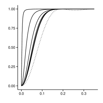
In conclusion the inverse multiquadric model is not very flexible in terms of the repulsiveness it can cover. However, for other choices of $\tau$ the situation appears to be much better. Figure 2 shows the pair correlation function for different values of $\tau$ for $d=2$ when $\delta$ is chosen such that $\eta_{\textup{max},2}=400$ together with the most repulsive DPP with $\eta=400$. The figure suggests that the models become more repulsive when $\tau\to\infty$ with $\delta\to 0$ appropriately chosen to keep $\eta_{\textup{max},2}$ fixed, and based on the figure we conjecture that a limiting model exists, but we have not been able to prove this. The simulated realization in the middle panel of Figure 1 gives the qualitative impression that the multiquadric model can obtain a degree of repulsiveness that almost reaches the most repulsive DPP though the corresponding pair correlation functions can easily be distinguished in Figure 2. To calculate $\eta_{\textup{max},2}$ we simply use (4.30) and (4.14).

4.3.3 Spherical, Askey, and Wendland covariance functions

Table 1 shows special cases of Askey’s truncated power function and $C^{2}$-Wendland and $C^{4}$-Wendland correlation functions when $d\leq 3$ (here, for any real number, $x_{+}=x$ if $x\geq 0$, and $x_{+}=0$ if $x<0$). Note that a scale parameter $c$ can be included, where for the $C^{2}$ and $C^{4}$ Wendland correlation functions, $c\in(0,2\pi]$ and $c$ defines the compact support of these correlation functions, and where for the Askey’s truncated power function, $c>0$. Notice that these correlation functions are of class $\Psi_{3}^{+}$, they are compactly supported for $c<\pi$, and compared to the Askey and Wendland correlation functions in [10, Table 1] they are the most repulsive cases. Appendix E describes how the one-Schoenberg coefficients listed in Table 1 can be derived. The one-Schoenberg coefficients can then be used to obtain the 3-Schoenberg coefficients, cf. [10, Corollary 3]. Moreover, the spherical correlation function

$$\psi(s)=\left(1+\frac{s}{2c}\right)\left(1-\frac{s}{c}\right)_{+}^{2},\qquad 0\leq s\leq\pi,$$

is of class $\Psi_{3}^{+}$, and the proof of [10, Lemma 2] specifies its one-Schoenberg coefficients and hence the 3-Schoenberg coefficients can also be calculated. Plots (omitted here) of the corresponding Mercer coefficients for $d\in\{1,3\}$ show that DPPs with the kernel specified by the Askey, $C^{2}$-Wendland, $C^{4}$-Wendland, or spherical correlation function are very far from the most repulsive case.

Table 1: Special cases of Askey’s truncated power function and $C^{2}$-Wendland and $C^{4}$-Wendland correlation functions when $d\leq 3$ and $c=1$, where the two last columns specify the corresponding one-Schoenberg coefficients. For a general value of a scale parameter $c>0$ (with $c\leq 2\pi$ in case of the Wendland functions), in the expressions for $\psi$, $s$ should be replaced by $s/c$, while in the expressions for $\beta_{\ell,1}$, $\ell$ should be replaced by $c\ell$ and the one-Schoenberg coefficient should be multiplied by $c$.

	$\psi$	$\beta_{\ell,1}$ ($\ell=1,2,\ldots$)	$\beta_{0,1}$
Askey	$(1-s)_{+}^{3}$	$\frac{6(\ell^{2}+2\cos(\ell)-2)}{\pi\ell^{4}}$	$\frac{1}{4\pi}$
$C^{2}$-Wendland	$(1-s)_{+}^{4}(4s+1)$	$\frac{240(\ell^{2}+\ell\sin(\ell)+4\cos(\ell)-4)}{\pi\ell^{6}}$	$\frac{1}{6\pi}$
$C^{4}$-Wendland	$\frac{1}{3}(1-s)_{+}^{6}(s(35s+18)+3)$	$\frac{8960(-4\ell(\ell^{2}-18)+3(\ell^{2}-35)\sin(\ell)+33\ell\cos(\ell))}{\pi\ell^{9}}$	$\frac{4}{27\pi}$

4.3.4 A flexible spectral model

Suppose that the kernel of the DPP has Mercer coefficients

$$\lambda_{\ell,d}=\frac{1}{1+\beta\exp\left((\ell/\alpha)^{\kappa}\right)}\,,\qquad\ell=0,1,\ldots,$$

where $\alpha>0$, $\beta>0$, and $\kappa>0$ are parameters. Since all $\lambda_{\ell,d}\in(0,1)$, the DPP is well defined and has a density specified by (3.8). Since its kernel is positive definite, all finite subsets of $\mathbb{S}^{d}$ are feasible realizations of the DPP. The mean number of points $\eta$ may be evaluated by numerical methods.

The most repulsive DPP is a limiting case: For any $n\in\{0,1,\ldots\}$, let $\eta_{0}=\sum_{\ell=0}^{n}m_{\ell,d}$, $\alpha=n$, and $\beta=1/(n\kappa)$. Then, as $\kappa\rightarrow\infty$, $\beta\exp\left((\ell/\alpha)^{\kappa}\right)$ converges to 0 for $\ell\leq n$ and to $\infty$ for $\ell>n$. Thus $\lambda_{\ell,d}\rightarrow 1$ for $\ell\leq n$, $\lambda_{\ell,d}\rightarrow 0$ for $\ell>n$, and $\eta\rightarrow\eta_{0}$. This limiting case corresponds to the case of $\bm{X}^{(\eta_{0})}$, the most repulsive DPP consisting of $\eta_{0}$ points.

Also the homogeneous Poisson process is a limiting case: Note that for fixed $d\geq 1$, the multiplicities $m_{\ell,d}$ given by (4.4) satisfy the asymptotic estimate $m_{l,d}\sim(1+\ell)^{d-1}$ as $\ell\rightarrow\infty$ (again $f_{1}(\ell)\sim f_{2}(\ell)$ means that $c_{d}\leq f_{1}(\ell)/f_{2}(\ell)\leq C_{d}$ where $C_{d}\geq c_{d}$ are positive constants). Hence,

$$\eta=\sum_{\ell=0}^{\infty}m_{\ell,d}\lambda_{\ell,d}\sim\sum_{\ell=0}^{\infty}(1+\ell)^{d-1}\frac{1}{1+\beta\exp((\ell/\alpha)^{\kappa})}.$$

Now, for a given value $\eta=\eta_{0}>0$, put $\kappa=d$ and $\alpha=(\eta_{0}\beta)^{1/d}$. Then, for sufficiently large $\beta$,

$$\sum_{\ell=0}^{\infty}(1+\ell)^{d-1}\frac{1}{1+\beta\exp((\ell/\alpha)^{d})}\sim\eta_{0}.$$

Consequently, as $\beta\rightarrow\infty$, we obtain $\eta\sim\eta_{0}$, while

$$\lambda_{\ell,d}\rightarrow 0,\qquad\ell=0,1,2\ldots$$

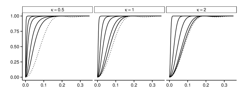
The model covers a wide range of repulsiveness as indicated in Figure 3. Compared to the multiquadric model in Figure 2 we immediately notice that even with a moderate value of the exponent parameter ($\kappa=2$) this model allows us to come much closer to the most repulsive DPP. The drawback of this model is that neither the intensity nor the pair correlation function is know analytically. To approximate each pair correlation function we have used (4.5) with $\beta_{\ell,d}=\lambda_{\ell,d}m_{\ell,d}/\eta$ where $\eta$ is evaluated numerically.

Figure 3: Approximate pair correlation functions for DPP models with $d=2$. Within each panel the full lines from left to right correspond to spectral models with $\beta=100,\allowbreak 5,\allowbreak 1,\allowbreak 0.1,\allowbreak 0.01$ and $\alpha$ chosen such that $\eta\approx 400$ given the value of $\kappa$ as indicated in the figure. The dotted line corresponds to the most repulsive DPP with $\eta=400$.

4.3.5 Matérn covariance functions

The Matérn correlation function is of class $\Psi_{\infty}^{+}$ and given by

$$\psi(s)=\frac{2^{1-\nu}}{\Gamma(\nu)}\left(\frac{s}{c}\right)^{\nu}K_{\nu}\left(\frac{s}{c}\right),\qquad 0\leq s\leq\pi,$$

where $\nu\in(0,\frac{1}{2}]$ and $c>0$ are parameters and $K_{\nu}$ denotes the modified Bessel function of the second kind of order $\nu$, see [10, Section 4.5]. For $\nu=\frac{1}{2}$, $\psi(s)=\exp(-s/c)$ is the exponential correlation function. The nomenclature Matérn function might be considered a bit ambitious here, since we are considerably restricting the parameter space for $\nu$. Indeed, it is true that any value of $\nu>0$ can be used when replacing the great circle distance with the chordal distance, but the use of this alternative metric is not contemplated in the present work.

Suppose $R_{0}=\psi$ is (the radial part of) the kernel for an isotropic DPP. Then the DPP becomes more and more repulsive as the scale parameter $c$ or the smoothness parameter $\nu$ increases, since $g_{0}$ then decreases. In the limit, as $c$ tends to 0, $g_{0}$ tends to the pair correlation function for a Poisson process. It can also be verified that $g_{0}$ increases as $\nu$ decreases.

For $\nu=\frac{1}{2}$, $g_{0}(s)=1-\exp(-2s/c)$, so $g_{0}^{\prime}(0)=2/c>0$ and hence the DPP is locally less repulsive than any other DPP with the same intensity and such that the slope for the tangent line of its pair correlation function at $s=0$ is at most $2/c$. For $\nu<\frac{1}{2}$, $g_{0}^{\prime}(0)=\infty$. That is, a singularity shows up at zero in the derivative of $R_{0}$, which follows from the asymptotic expansions of $K_{\nu}$ given in [1, Chapter 9]. Hence, the DPP is locally less repulsive than any other DPP with the same intensity and with a finite slope for the tangent line of its pair correlation function at $s=0$. Consequently, the variance condition (4.21) is violated for all $\nu\in(0,1/2]$.

We are able to derive a few more analytical results: For $d=1$ and $\nu=\frac{1}{2}$, (4.9) yields

$$\beta_{0,1}=\frac{c}{\pi}\left\{1-\exp\left(-\frac{\pi}{c}\right)\right\},$$

and

$$\beta_{\ell,1}=\frac{2}{\pi}\left\{1+(-1)^{\ell+1}\exp\left(-\frac{\pi}{c}\right)\right\}\frac{c}{1+c^{2}\ell^{2}}\,,\qquad\ell=1,2,\ldots$$

Hence

$$\eta_{\textup{max},1}=\frac{\pi}{c}\,\frac{1}{1-\exp\left(-\frac{\pi}{c}\right)}\,,$$

which is a decreasing function of $c$, with range $(1,\infty)$.

Incidentally, [11] introduced what they call a circular Matérn covariance function and which for $d=1$ has Mercer coefficients

$$\lambda_{\ell,1}=\frac{\sigma^{2}}{\left(\alpha^{2}+\ell^{2}\right)^{\nu+1/2}},\qquad\ell=0,1,\ldots,$$

where $\sigma>0$, $\nu>0$, and $\alpha>0$ are parameters. Consider a DPP with the circular Matérn covariance function as its kernel and with $d=1$. This is well defined exactly when $\sigma\leq\alpha^{\nu+1/2}$. Then the mean number of points is

$$\eta=\sum_{\ell=-\infty}^{\infty}\frac{\sigma^{2}}{\left(\alpha^{2}+\ell^{2}\right)^{\nu+1/2}},$$

which is bounded by

$$\eta_{\textup{max},1}=\sum_{\ell=-\infty}^{\infty}\frac{1}{\left(1+(\ell/\alpha)^{2}\right)^{\nu+1/2}}.$$

When $\nu$ is a half-integer, the kernel and hence also $\eta$ and $\eta_{\textup{max},1}$ are expressible on closed form, see [11]. Finally, considering the case $\sigma=\alpha^{\nu+1/2}$ (equivalently $\eta=\eta_{\textup{max},1}$), then

$$\lambda_{\ell,1}=\frac{1}{\left(1+(\ell/\alpha)^{2}\right)^{\nu+1/2}},\qquad\ell=0,1,\ldots,$$

and we see that the DPP never reaches the most repulsive DPP except in the limit where $\eta_{\textup{max},1}\rightarrow 1$.

Figure 4: Pair correlation functions for DPP models with $d=1$. Full lines from left to right correspond to circular Matérn models with $\nu=0.5,1,2,10$, $\sigma=\alpha^{\nu+1/2}$, and $\alpha=31.8,50,75,176.2$ chosen such that $\eta=\eta_{\textup{max},1}\approx 100$. The dotted line corresponds to the most repulsive DPP with $\eta=100$.

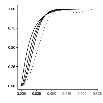
Figure 4 shows four different pair correlation functions corresponding to different values of $\nu$ for the circular Matérn model with $\eta=\eta_{\textup{max},1}$ (i.e. $\sigma=\alpha^{\nu+1/2}$). For values $\nu>10$ the curves become almost indistinguishable from the one with $\nu=10$, so we have omitted these from the figure. The left most curve ($\nu=1/2$) is in fact almost numerically identical to the ordinary Matérn model introduced above with $\nu=1/2$ and $\eta_{\textup{max},1}=100$. Since $\nu=1/2$ corresponds to the most repulsive ordinary Matérn model we see that the circular Matérn model covers a much larger degree of repulsiveness than the ordinary Matérn model.

5 Concluding remarks

In this paper, we have considered determinantal point processes (DPPs) on the $d$-dimensional unit sphere $\mathbb{S}^{d}$. We have shown that DPPs on spheres share many properties with DPPs on $\mathbb{R}^{d}$, and these properties are simpler to establish and to exploit for statistical purposes on $\mathbb{S}^{d}$ due to compactness of the space.

For DPPs with a distribution specified by a given kernel (a complex covariance function of finite trace class and which is square integrable), we have developed a suitable Mercer (spectral) representation of the kernel. In particular, we have studied the case of DPPs with a distribution specified by a continuous isotropic kernel. Such kernels can be expressed by a Schoenberg representation in terms of countable linear combination of Gegenbauer polynomials, and a precise connection between the Schoenberg representation and the Mercer representation has been presented. Furthermore, the trade-off between the degree of repulsiveness and the expected number of points in the model has been established, and the ‘most repulsive isotropic DPPs’ have been identified.

We have used the connection between the Schoenberg and Mercer representations to construct a number of tractable and flexible parametric models for isotropic DPPs. We have considered two different modelling approaches where we either work with a closed form expression for the correlation function $\psi$ or with its Mercer/spectral representation. With the former approach the multiquadric model seems to be the most promising model with some flexibility, and the closed form expression for $\psi$ opens up for computationally fast moment based parameter estimation in future work. The two main drawbacks is that this class cannot cover the most extreme cases of repulsion between points and simulation requires truncation of a (possibly) infinite series, which in some cases may be problematic. However, in our experience the truncation works well in the most interesting cases when we are not too close to a Poisson point process. In that case the Schoenberg coefficients decay very slowly and it becomes computationally infeasible to accurately approximate the $d$-Schoenberg coefficients. The flexible spectral model we have developed overcomes these two drawbacks. It covers the entire range of repulsiveness from the lack of repulsion in the Poisson case to the most repulsive DPP, and it is straightforward to generate simulated realizations from this model. The main drawback here is that the intensity and pair correlation function only can be evaluated numerically making moment based inference more difficult, and the parameters of the model may be harder to interpret.

We defer for another paper how to construct anisotropic models and to perform statistical inference for spatial point pattern datasets on the sphere. In brief, smooth transformations and independent thinnings of DPPs results in new DPPs, whereby anisotropic DPPs can be constructed from isotropic DPPs. For $d=2$ particular forms for anisotropy should also be investigated such as axial symmetry (see e.g. [16, 13]) meaning that the kernel is invariant to shifts in the polar longitude.

We have developed software in the R language [23] to handle DPPs on the sphere as an extension to the spatstat package [2] and it will be released in a future version of spatstat. Until official release in spatstat the code can be obtained by sending an email to the authors. Some figures have been created with the R package ggplot2 [29].

Acknowledgments

Supported by the Danish Council for Independent Research | Natural Sciences, grant 12-124675, “Mathematical and Statistical Analysis of Spatial Data”, by Proyecto Fondecyt Regular 1130647 from the Chilean Ministry of Education, and by the Centre for Stochastic Geometry and Advanced Bioimaging, funded by a grant (8721) from the Villum Foundation.

Appendix A Simulation algorithm

As mentioned in the comment to Theorem 3.22 we need to simulate points sequentially given the previously generated points. This is done by rejection sampling from a uniform instrumental distribution as described in [18, 19] which requires an upper bound on the squared modulus of the eigenfunctions. Specifically, when $d=2$ (using the notation from equation (4.10) in Theorem 4.1) we can use the bound

$$|Y_{l,k,2}(\vartheta,\varphi)|^{2}\leq\frac{2l+1}{4\pi}\frac{(l-|k|)!}{(l+|k|)!}\quad\text{for all }(\vartheta,\varphi)\in[0,\pi]\times[0,2\pi).$$

Appendix B Eigenvalues for nonnegative $\psi(s)$

Suppose that $\psi(s)$ is nonnegative. Then $\tilde{\psi}(x):=\psi(\arccos x)$ is nonnegative and according to (4.5)

$$\tilde{\psi}(x)=\sum_{\ell=0}^{\infty}\beta_{\ell,d}\frac{{\cal C}_{\ell}^{(\frac{d-1}{2})}(x)}{{\cal C}_{\ell}^{(\frac{d-1}{2})}(1)},\qquad-1\leq x\leq 1.$$

We use the orthogonality of the Gegenbauer polynomials with respect to the measure $(1-x^{2})^{\frac{d-2}{2}}\,\mathrm{d}x$ on $[-1,1]$, see [1, p. 774], to obtain

$$\beta_{\ell,d}={\cal C}_{\ell}^{(\frac{d-1}{2})}(1)\cdot\frac{l!\,\left(2l+d-1\right)\left[\Gamma\left(\frac{d}{2}-\frac{1}{2}\right)\right]^{2}}{\pi\,{2}^{3-d}\Gamma\left(l+d-1\right)}\int_{-1}^{1}\tilde{\psi}(x){\cal C}_{\ell}^{(\frac{d-1}{2})}(x)(1-x^{2})^{\frac{d-2}{2}}\,\mathrm{d}x.$$

It follows that

$$\alpha_{\ell,d} =\frac{\sigma_{d}\cdot\beta_{\ell,d}}{m_{\ell,d}}$$

$$=\sigma_{d}\cdot\frac{[{\cal C}_{\ell}^{(\frac{d-1}{2})}(1)]^{2}}{m_{\ell,d}}\cdot\frac{l!\,\left(2l+d-1\right)\left[\Gamma\left(\frac{d}{2}-\frac{1}{2}\right)\right]^{2}}{\pi\,{2}^{3-d}\Gamma\left(l+d-1\right)}\int_{-1}^{1}\tilde{\psi}(x)\frac{{\cal C}_{\ell}^{(\frac{d-1}{2})}(x)}{{\cal C}_{\ell}^{(\frac{d-1}{2})}(1)}(1-x^{2})^{\frac{d-2}{2}}\,\mathrm{d}x$$

$$={\frac{2{\pi}^{d/2}}{\Gamma\left(d/2\right)}}\int_{-1}^{1}\tilde{\psi}(x)\frac{{\cal C}_{\ell}^{(\frac{d-1}{2})}(x)}{{\cal C}_{\ell}^{(\frac{d-1}{2})}(1)}(1-x^{2})^{\frac{d-2}{2}}\,\mathrm{d}x.$$ (B.1)

It is known that $\|{\cal C}_{\ell}^{(\frac{d-1}{2})}(x)/{{\cal C}_{\ell}^{(\frac{d-1}{2})}(1)}\|_{L^{\infty}}\leq 1$ for all $\ell\geq 0$, see [28, Theorem 7.32.1], and ${\cal C}_{0}^{(\frac{d-1}{2})}(x)\equiv 1$. Combined with the fact that $\tilde{\psi}(x)(1-x^{2})^{\frac{d-2}{2}}$ is nonnegative on $[-1,1]$, it follows directly from Hölder’s inequality applied to (B.1) that

$$\sup_{\ell}\alpha_{\ell,d}=\alpha_{0,d}={\frac{2{\pi}^{d/2}}{\Gamma\left(d/2\right)}}\int_{-1}^{1}\tilde{\psi}(x)(1-x^{2})^{\frac{d-2}{2}}\,\mathrm{d}x.$$

In fact, we may also conclude that $\alpha_{0,d}>\alpha_{\ell,d}$, $\ell\geq 1$, since $|{\cal C}_{\ell}^{(\frac{d-1}{2})}(x)/{{\cal C}_{\ell}^{(\frac{d-1}{2})}(1)}|<1$ on a set of positive measure, which can be deduced from the orthogonality of the Gegenbauer system.

Appendix C Proof of Theorem 4.2(b)

For $d\geq 2$, we use [17, Equation (2.7)] to obtain

$$x^{\ell}=\sum_{\begin{subarray}{c}n=0\\ n-\ell\equiv 0\!\!\!\pmod{2}\end{subarray}}^{\ell}\frac{(2n+d-1)(\ell!)\Gamma(\frac{d-1}{2})}{2^{\ell+1}\{(\frac{\ell-n}{2})!\}\Gamma(\frac{\ell+n+d+1}{2})}\mathcal{C}_{n}^{(\frac{d-1}{2})}(x),\qquad x\in[-1,1].$$

Hence, for any function $\psi$ admitting the expansion (4.16) we obtain an associated Schoenberg expansion of the type

$$\psi(s) =\sum_{\ell=0}^{\infty}\beta_{\ell}\Bigl{(}\sum_{\begin{subarray}{c}n=0\\ n-\ell\equiv 0\!\!\!\pmod{2}\end{subarray}}^{\ell}\frac{(2n+d-1)(\ell!)\Gamma(\frac{d-1}{2})}{2^{\ell+1}\{(\frac{\ell-n}{2})!\}\Gamma(\frac{\ell+n+d+1}{2})}\mathcal{C}_{n}^{(\frac{d-1}{2})}(\cos s)\Bigr{)}$$

$$=\sum_{n=0}^{\infty}\Bigl{(}\sum_{\begin{subarray}{c}\ell=n\\ n-\ell\equiv 0\!\!\!\pmod{2}\end{subarray}}^{\infty}\beta_{\ell}\frac{(2n+d-1)(\ell!)\Gamma(\frac{d-1}{2})}{2^{\ell+1}\{(\frac{\ell-n}{2})!\}\Gamma(\frac{\ell+n+d+1}{2})}\mathcal{C}_{n}^{{(\frac{d-1}{2})}}(1)\Bigr{)}\frac{\mathcal{C}_{n}^{(\frac{d-1}{2})}(\cos s)}{\mathcal{C}_{n}^{{(\frac{d-1}{2})}}(1)},$$

whereby (4.17) is seen to be true for $d\geq 2$, since $\mathcal{C}_{n}^{{(\frac{d-1}{2})}}(1)=\binom{n+d-2}{n}$. For $d=1$ we use a similar argument based on the power reduction formula,

$$\cos^{\ell}s =2^{-\ell}\sum_{\begin{subarray}{c}n=0\\ n-\ell\equiv 0\!\!\!\pmod{2}\end{subarray}}^{\ell}\big{(}2-\delta_{n,0}\delta_{\ell\!\!\!\!\pmod{2},0}\big{)}\binom{\ell}{\frac{\ell-n}{2}}\cos(ns)$$

$$=2^{-\ell}\sum_{\begin{subarray}{c}n=0\\ n-\ell\equiv 0\!\!\!\pmod{2}\end{subarray}}^{\ell}\big{(}2-\delta_{n,0}\delta_{\ell\!\!\!\!\pmod{2},0}\big{)}\binom{\ell}{\frac{\ell-n}{2}}\mathcal{C}_{n}^{(0)}(\cos s).$$

Appendix D Proof of Theorem 4.4

This appendix verifies (a)–(c) in Theorem 4.4.

(a) It follows straightforwardly from (2.1)–(2.2) that

$$I(g_{0})=\frac{1}{\eta}-\frac{\text{Var}(\#\bm{X})}{\eta^{2}}.$$

Considering independent Bernoulli variables $B_{\ell,k,d}$ with parameters $\lambda_{\ell,d}$ for $k\in\mathcal{K}_{\ell,d}$ and $\ell=0,1,\ldots$, cf. Theorem 3.2(b) and (4.12), we obtain

$$\text{Var}(\#\bm{X})=\sum_{\ell=0}^{\infty}m_{\ell,d}\lambda_{\ell,d}\left(1-\lambda_{\ell,d}\right).$$

Thereby (4.20) follows.

(b)–(c) The case $d=1$ is left for the reader. Now suppose $d\geq 2$. Consider $g_{0}=1-R_{0}^{2}$, with Schoenberg representation

$$R_{0}(s)=\sum_{\ell=0}^{\infty}\beta_{\ell,d}\frac{\mathcal{C}_{\ell}^{(\frac{d-1}{2})}(\cos s)}{\mathcal{C}_{\ell}^{(\frac{d-1}{2})}(1)}.$$ (D.1)

We have $R_{0}(0)=1$,

$$\frac{\mathrm{d}\mathcal{C}_{\ell}^{(\frac{d-1}{2})}(\cos s)}{\mathrm{d}s}=-(d-1)\sin s\,\mathcal{C}_{\ell-1}^{(\frac{d+1}{2})}(\cos s)\,,$$

and

$$\bigg{|}\frac{(d-1)\sin s\,\mathcal{C}_{\ell-1}^{(\frac{d+1}{2})}(\cos s)}{\mathcal{C}_{\ell}^{(\frac{d-1}{2})}(1)}\bigg{|}\leq(d-1)\frac{\binom{\ell+d-1}{\ell-1}}{\binom{\ell+d-2}{\ell}}=\frac{\ell(\ell+d-1)}{d},$$

see [24, Chapter 17]. From this and the variance condition (4.21) we deduce that termwise differentiation of the right-hand side of (D.1) yields $R_{0}^{\prime}(s)$. In particular, $R_{0}^{\prime}(0)=0$, and so $g^{\prime}_{0}(0)=0$. Further, for $s=0$,

$$\left[\frac{\mathrm{d}^{2}\mathcal{C}_{\ell}^{(\frac{d-1}{2})}(\cos s)}{\mathrm{d}s^{2}}\right]_{s=0}=\left[\ldots-(d-1)\cos s\,\mathcal{C}_{\ell-1}^{(\frac{d+1}{2})}(\cos s)\right]_{s=0}=-(d-1)\mathcal{C}_{\ell-1}^{(\frac{d+1}{2})}(1),$$

where ‘$\ldots$’ is a product involving the $\sin^{2}s$ term and hence is 0 at $s=0$. Therefore, using again (4.21) and the same justification of termwise differentiation as above,

$$g_{0}^{\prime\prime}(0)=-2R_{0}^{\prime\prime}(0)=2(d-1)\sum_{\ell=0}^{\infty}\beta_{\ell,d}\frac{\binom{\ell+d-1}{\ell-1}}{\binom{\ell+d-2}{\ell}}=\frac{2}{d}\sum_{\ell=0}^{\infty}\ell(\ell+d-1)\beta_{\ell,d}.$$

Thereby (4.22) is verified. Finally,

$$g_{0}^{\prime\prime}(0)=\frac{2}{d\eta}\sum_{\ell=1}^{\infty}\ell(\ell+d-1)m_{\ell,d}\lambda_{\ell,d}\,,$$

and since $\ell(\ell+d-1)m_{\ell,d},\ \ell=1,2,\ldots,$ is a strictly increasing sequence, we conclude that $\bm{X}^{(\eta)}$ is the unique locally most repulsive isotropic DPP.

Appendix E Askey and Wendland correlation functions

Consider the Askey function

$$\psi_{\nu}(t)=\left(1-t\right)_{+}^{\nu},\qquad t\geq 0,\qquad\nu>0.$$

Denote $\widetilde{\psi}_{\nu}$ the restriction of $\psi_{\nu}$ to the interval $[0,\pi]$. In fact $\psi_{\nu}$ is the radial part of an Euclidean isotropic correlation function defined on $\mathbb{R}^{d}$ if and only if $\nu\geq\frac{d+1}{2}$, cf. [31]. Gneiting [9] in his essay used instead the condition $\nu\geq\lfloor d/2+1\rfloor$. This means that the function $\varphi(\bm{x})=\psi_{\nu}(\lVert\bm{x}\rVert)$ for $\bm{x}\in\mathbb{R}^{d}$ is positive definite under the mentioned constraint on $\nu$. Additionally, $\varphi$ is compactly supported on the unit ball of $\mathbb{R}^{d}$, and it can be arbitrarily rescaled to any ball of $\mathbb{R}^{d}$ with radius $c>0$ by considering $\varphi(\cdot/c)$. Thus $\widetilde{\psi}_{\nu}\in\Psi_{3}^{+}$ provided $\nu\geq 2$, cf. [9, Theorem 3].

Wendland functions are obtained through application of the Montée operator [21] to Askey functions. The Montée operator is defined by

$${\cal I}\psi_{\nu}(t)=\frac{\int_{t}^{\infty}u\psi_{\nu}\left(\frac{u}{b}\right){\rm d}u}{\int_{0}^{\infty}u\psi_{\nu}\left(\frac{u}{b}\right){\rm d}u},\qquad t>0,$$

and we define for $k=1,2,\ldots$, $\psi_{\nu,k}$ as the $k$th iterated application of the Montée operator to $\psi_{\nu}$, and we set $\psi_{\nu,0}=\psi_{\nu}$. Arguments in Gneiting (2002) show that $\varphi(\bm{x})=\psi_{\nu,k}(\|\bm{x}\|)$, $\bm{x}\in\mathbb{R}^{d}$, is positive definite provided $\nu\geq\frac{d+1}{2}+k$. Thus, for $k=0,1,\ldots$, the restriction of $\psi_{\nu,k}$ to $[0,\pi]$, denoted $\widetilde{\psi}_{\nu,k}$, belongs to $\Psi_{3}^{+}$ provided $\nu\geq 2+k$.

We shall only work with the special case $\nu=\lfloor d/2+k+1\rfloor$, where it is possible to deduce a closed form for the associated spectral density, see [30]. We consider then the mapping $\widetilde{\psi}_{\nu,k}$ as the restriction to $[0,\pi]$ of $\psi_{\nu,k}$, $k=0,1,\ldots$. Note that for $d=1$, the one-Schoenberg coefficient for $\psi_{\nu,k}$ can be calculated straightforwardly from the Fourier transform (4.9) using partial integration. Thereby we obtain Table 1, where $\widetilde{\psi}_{\nu,0}$ is the Askey function, $\widetilde{\psi}_{\nu,1}$ is the $C^{2}$-Wendland function, and $\widetilde{\psi}_{\nu,2}$ is the $C^{4}$-Wendland function.

References

• [1] M. Abramowitz and I. Stegun. Handbook of Mathematical Functions. Dover Publications, 1965.
• [2] A. Baddeley, E. Rubak, and R. Turner. Spatial Point Patterns: Methodology and Applications with R. Chapman and Hall/CRC Press, London, 2015.
• [3] C. Berg and E. Porcu. From Schoenberg coefficients to Schoenberg functions. Constructive approximation. Constructive Approximation, 2016. To appear.
• [4] C. A. N. Biscio and F. Lavancier. Quantifying repulsiveness of determinantal point processes. Bernoulli, 22:2001–2028, 2016.
• [5] R. Cavoretto and A. De Rossi. Fast and accurate interpolation of large scattered data sets on the sphere. Journal of Computational and Applied Mathematics, 234:1505–1521, 2010.
• [6] F. Dai and Y. Xu. Approximation Theory and Harmonic Analysis on Spheres and Balls. Springer Monographs in Mathematics. Springer, New York, 2013.
• [7] D. J. Daley and E. Porcu. Dimension walks through Schoenberg spectral measures. Proceedings of the American Mathematical Society, 42:1813–1824, 2013.
• [8] J. Ginibre. Statistical ensembles of complex, quaternion, and real matrices. Journal of Mathematical Physics, 6:440–449, 1965.
• [9] T. Gneiting. Compactly supported correlation functions. Journal of Multivariate Analysis, 83:493–508, 2002.
• [10] T. Gneiting. Strictly and non-strictly positive definite functions on spheres. Bernoulli, 19:1327–1349, 2013.
• [11] J. Guinness and M. Fuentes. Isotropic covariance functions on spheres: Some properties and modeling considerations. Journal of Multivariate Analysis, 143:143–152, 2016.
• [12] A. Higuchi. Symmetric tensor spherical harmonics on the ${N}$-sphere and their application to the de Sitter group SO(${N}$,1). Journal of Mathematical Physics, 28:1553–1566, 1987.
• [13] M. Hitczenko and M. L. Stein. Some theory for anisotropic processes on the sphere. Statistical Methodology, 9:211–227, 2012.
• [14] J. B. Hough, M. Krishnapur, Y. Peres, and B. VirΓ g. Determinantal processes and independence. Probability Surveys, 3:206–229, 2006.
• [15] J. B. Hough, M. Krishnapur, Y. Peres, and B. VirΓ g. Zeros of Gaussian Analytic Functions and Determinantal Point Processes. American Mathematical Society, Providence, 2009.
• [16] A. H. Jones. Stochastic processes on a sphere. The Annals of Mathematical Statistics, 34:213–218, 1963.
• [17] D. S. Kim, T. Kim, and S.-H. Rim. Some identities involving Gegenbauer polynomials. Advances in Difference Equations, page 219, 2012.
• [18] F. Lavancier, J. MΓΈller, and E. Rubak. Determinantal point process models and statistical inference: Extended version. Technical report, available at arXiv:1205.4818, 2014.
• [19] F. Lavancier, J. MΓΈller, and E. Rubak. Determinantal point process models and statistical inference. Journal of Royal Statistical Society: Series B (Statistical Methodology), 77:853–877, 2015.
• [20] D. Marinucci and G. Peccati. Random Fields on the Sphere. Representation, Limit Theorems and Cosmological Applications. London Mathematical Society Lecture Notes Serie: 389. Cambridge University Press, Cambridge, 2011.
• [21] G. Matheron. The intrinsic random functions and their applications. Advances in Applied Probability, 5:439–468, 1973.
• [22] E. Porcu, M. Bevilacqua, and M. Genton. Spatio-temporal covariance and cross-covariance functions of the great circle distance on a sphere. Journal of the American Statistical Association, page Accepted., 2016.
• [23] R Core Team. R: A Language and Environment for Statistical Computing. R Foundation for Statistical Computing, Vienna, Austria, 2015.
• [24] E. D. Rainville. Special Functions. Chelsea Publishing Co., Bronx, N.Y., first edition, 1971.
• [25] F. Riesz and B. Sz.-Nagy. Functional Analysis. Dover Publications, New York, 1990.
• [26] I. J. Schoenberg. Positive definite functions on spheres. Duke Mathematical Journal, 9:96–108, 1942.
• [27] T. Shirai and Y. Takahashi. Random point fields associated with certain Fredholm determinants I: fermion, Poisson and boson point processes. Journal of Functional Analysis, 205:414–463, 2003.
• [28] G. SzegΕ‘. Orthogonal polynomials. American Mathematical Society, Providence, R.I., fourth edition, 1975. American Mathematical Society, Colloquium Publications, Vol. XXIII.
• [29] H. Wickham. ggplot2: Elegant Graphics for Data Analysis. Springer New York, 2009.
• [30] V. P. Zastavnyi. On the properties of Buhmann functions. Ukrainian Mathematical Journal, 58:1184–1208, 2006.
• [31] V. P. Zastavnyi and R. M. Trigub. Positive-definite splines of special form. Sbornik: Mathematics, 193:1771–1800, 2002.