The HADES RV Programme with HARPS-N@TNG
GJ 3998: An early M-dwarf hosting a system of Super-Earths

Abstract

Context. Many efforts to detect Earth-like planets around low-mass stars are presently devoted in almost every extra-solar planet search. M dwarfs are considered ideal targets for Doppler radial velocity searches because their low masses and luminosities make low-mass planets orbiting in their habitable zones more easily detectable than those around higher mass stars. Nonetheless, the statistics of frequency of low-mass planets hosted by low mass stars remains poorly constrained.

Aims. Our M-dwarf radial velocity monitoring with HARPS-N within the GAPS (Global architectures of Planetary Systems) – ICE (Institut de Ciències de l’Espai/CSIC-IEEC) – IAC (Instituto de Astrofísica de Canarias) project can provide a major contribution to the widening of the current statistics through the in-depth analysis of accurate radial velocity observations in a narrow range of spectral sub-types (79 stars, between dM0 to dM3). Spectral accuracy will enable us to reach the precision needed to detect small planets with a few earth masses. Our survey will bring a contribute to the surveys devoted to the search for planets around M-dwarfs, mainly focused on the M-dwarf population of the northern emisphere, for which we will provide an estimate of the planet occurence.

Methods. We present here a long duration radial velocity monitoring of the M1 dwarf star GJ 3998 with HARPS-N to identify periodic signals in the data. Almost simultaneous photometric observations were carried out within the APACHE and EXORAP programs to characterize the stellar activity and to distinguish from the periodic signals those due to activity and to the presence of planetary companions. We run an MCMC simulation and use Bayesian model selection to determine the number of planets in this system, to estimate their orbital parameters and minimum masses and for a proper treatment of the activity noise.

Results. The radial velocities have a dispersion in excess of their internal errors due to at least four superimposed signals, with periods of 30.7, 13.7, 42.5 and 2.65 days. Our data are well described by a 2-planet Keplerian (13.7 d and 2.65 d) and 2 sinusoidal functions (stellar activity, 30.7 d and 42.5 d) fit. The analysis of spectral indices based on Ca II H & K and H$\alpha$ lines demonstrates that the periods of 30.7 and 42.5 days are due to chromospheric inhomogeneities modulated by stellar rotation and differential rotation. This result is supported by photometry and is consistent with the results on differential rotation of M stars obtained with $Kepler$. The shorter periods of $13.74\pm\,0.02\,d$ and $2.6498\pm\,0.0008\,d$ are well explained with the presence of two planets, with minimum masses of $6.26^{+0.79}_{-0.76}$  M_⊕ and $2.47\pm\,0.27$  M_⊕ and distances of 0.089 AU and 0.029 AU from the host, respectively.

1 Introduction

In the two decades since the discovery of the first giant planetary mass companion to a main sequence star (Mayor & Queloz, 1995) the search for and characterization of extrasolar planets has quickly developed to become a major field of modern-day astronomy. Thanks to concerted efforts with a variety of observational techniques (both from the ground and in space), thousands of confirmed and candidate planetary systems are known to-date (e.g., http://www.exoplanet.eu - Schneider et al., 2011), encompassing orders of magnitude in mass and orbital separation. The frontier today is being pushed ever closer to the identification of potentially habitable small-mass planets with a well-determined rocky composition similar to Earth’s. Planetary systems harboring objects with these characteristics are likely to be discovered first around primaries with later spectral types than the Sun’s.

Stars in the lower main sequence (M dwarfs) constitute the vast majority ($>70-75\%$) of all stars, both in the Solar neighbourhood and in the Milky Way as a whole (Henry et al., 2006; Winters et al., 2015). They are particularly promising targets for exoplanet search programs for a number or reasons. In particular, the favourable mass and radius ratios lead to readily detectable radial-velocity (RV) and transit signals produced by terrestrial-type planets. Furthermore, the low luminosities of M dwarfs imply that the boundaries of their habitable zones (HZ) are located at short separations (typically between 0.02 AU and 0.2 AU, see e.g. Mandell et al., 2007), making rocky planets orbiting within them more easily detectable with present-day observing facilities than those around more massive stars (e.g. Charbonneau & Deming, 2007). Finally, the favorable planet-star contrast ratios for small stars enable the best opportunities in the near future for detailed characterization studies of small planets and their atmospheres (e.g. Seager & Deming, 2010).

Figure 1: Radial velocity (top) and activity indices H$\alpha$ (middle) and $S$ index (bottom) time series for GJ 3998 measured with the TERRA pipeline.

While the first planets discovered around M dwarfs were Jovian-type companions (Delfosse et al., 1998; Marcy et al., 1998, 2001), it is now rather well observationally established that their frequency is lower than that of giant planets around solar-type hosts (e.g. Sozzetti et al., 2014), and references therein), a result understood within the context of the core-accretion formation model (e.g. Laughlin et al., 2004). The most recent evidence gathered by RV surveys and ground-based as well as space-borne transit search programs points instead towards the ubiquitousness of small (in both mass and radius) companions around M dwarfs. The outstanding photometric dataset of transit candidates around early M dwarfs from the Kepler mission has allowed Gaidos et al. (2016) and Dressing & Charbonneau (2015) to derive cumulative occurrence rates of $2.3\pm 0.3$ and $2.5\pm 0.2$ planets with $1-4$ R_⊕ for orbital periods $P$ shorter than 180 days and 200 days, respectively. Approximately one in two early M-type stars appears to host either an Earth-sized ($1-1.5$ R_⊕) or a Super Earth ($1.5-2.0$ R_⊕) planet (Dressing & Charbonneau, 2015) with an orbital period $<50$ days. Based on different recipes for the definition of the HZ boundaries and planetary atmospheric properties, Kopparapu (2013) and Dressing & Charbonneau (2015) obtain frequency estimates of potentially habitable terrestrial planets ($1-2$ R_⊕) around the Kepler early M-dwarf sample $\eta_{\oplus}=48^{+12}_{-24}$% and $\eta_{\oplus}=43^{+14}_{-9}$%, respectively. The inference from RV surveys of early- and mid-M dwarfs instead indicates $0.88^{+0.55}_{-0.19}$ Super Earth planets per star with $P<100$ d and $m\sin i=1-10$ M_⊕, and a frequency of such planets orbiting within the host’s HZ $\eta_{\oplus}=41^{+54}_{-13}$% (Bonfils et al., 2013). The $\eta_{\oplus}$ estimates from Doppler and transit surveys thus seem to be in broad agreement. However, $a)$ the uncertainties associated to these occurrence rate estimates are still rather large, and $b)$ the known compositional degeneracies in the mass-radius parameter space for Super Earths (e.g. Rogers & Seager, 2010) make the mapping between the $\eta_{\oplus}$ estimates based on (minimum) mass and radius not quite straightforward. Any additional constraints coming from ongoing and upcoming planet detection experiments targeting M dwarfs are then particularly valuable.

We present here high-precision, high-resolution spectroscopic measurements of the bright ($V=10.83$ mag) M1 dwarf GJ 3998, gathered with the HARPS-N spectrograph (Cosentino et al., 2012) on the Telescopio Nazionale Galileo (TNG) as part of an RV survey for low-mass planets around a sample of northern-hemisphere early-M dwarfs. The HADES (HArps-n red Dwarf Exoplanet Survey) observing programme is the result of a collaborative effort between the Italian Global Architecture of Planetary Systems (GAPS, Covino et al., 2013; Desidera et al., 2013; Poretti et al., 2016) Consortium, the Institut de Ciències de l’Espai de Catalunya (ICE), and the Instituto de Astrofísica de Canarias (IAC). Analysis of the Doppler time-series, spanning $\sim 2.4$ years, reveals the presence of a systems of two Super Earths orbiting at 0.029 AU and 0.089 AU from the central star. After a short presentation of the HADES RV programme, in Sect. 2 we describe the observations and reduction process and in Sect. 3 we summarize the atmospheric, physical and kinematic properties of GJ 3998. In Sect. 4 we describe the RV analysis and discuss the impact of stellar activity. Sect. 5 presents the analysis and results of a multi-site photometric monitoring campaign. In Sect. 6 we describe the Bayesian analysis, the model selection and derive the system parameters. We summarize our findings and conclude in Sect. 7.

2 The HADES RV programme

The HADES RV programme has completed the 6^th semester of observations. The complete original sample is composed by 106 stars, ranging from dM0 to dM3 spectral type, selected from the (Lépine & Gaidos, 2013) and Palomar/Michigan State University (PMSU, Reid et al., 1995) catalogs, with the additional criterion to be part of the APACHE catalog (Sozzetti et al., 2013), with a visible magnitude lower than 12 and with a high number of Gaia mission scans. The M stars are photometrically monitored also by the EXORAP program at Serra La Nave. These selection criteria are meant to reach a good characterization of the systems. From the complete sample, 27 stars were rejected during the first semester of observations (binary systems, fast rotators, peculiar stars, high activity, earlier type stars and/or wrong spectral type). Some of the targets ($\approx$ 15% of the cleaned sample) have already more than 80 RV points, with an excellent precision (1-1.8 m s^-1 at V$\approx$ 10-11). The star GJ 3998 emerged among several possible candidates, since it shows clear periodic signals consistent with the presence of planets.
The statistical analysis of the capability of our survey is the purpose of the second paper of the HADES series (Perger et al. 2016, submitted). It is focused on simulating the planet detection rates on low-mass stars and predicting the number of planets likely to be detected, using the most recent planet occurrence statistics applied to our stellar sample and the actual observation times of our survey. The simulations performed by Perger et al., show, as first statistical outcomes, that: 1) the observations of the HADES program analyzed to date should enable the detection of $2.3\,\pm\,1.6$  planets (3.6% detection rate), in agreement with our findings; 2) with 120 obs/star we are able to detect around 10% of the distributed planets; 3) the optimum average number of observations per target, in case of time-limited survey, is around 35, for the case of early M-dwarf sample and exposure times of 900s (for further information see Perger et al. 2016, submitted, and references therein).

GJ 3998 has been monitored from BJD = 2 456 439.6 (26th of May 2013) to BJD = 2 457 307.8 (12th of October 2015). We obtained a total of 136 data points spanning 869 days (Fig. 1). The spectra were obtained at high resolution (R $\sim$  115 000) with the optical echelle spectrograph HARPS-N with exposure times of 15 minutes and average signal-to-noise ratio (S/N) of 45 at 5500 Å. Of the 136 epochs, 76 were obtained within the GAPS time and 60 within the Spanish time. Observations were gathered without the simultaneous Th-Ar calibration, which is usually used to correct for instrumental drifts during the night. This choice avoided the contamination of the Ca II H & K lines, which are particularly important for the stellar activity analysis of M dwarfs (Giampapa et al., 1989; Forveille et al., 2009; Lovis et al., 2011). The M-type stars were observed by the Italian team in conjunction with other GAPS targets, which used the Th-Ar simultaneous calibration, thus we estimated the drift data between the two fibers (star and reference calibration) for each night from these observations, and evaluated the interpolated drift for GJ 3998.

Data reduction and spectral extraction were performed using the Data Reduction Software (DRS v3.7, Lovis & Pepe, 2007). RVs were measured by means of a weighted cross-correlation function (CCF) with the M2 binary mask provided with the DRS (Baranne et al., 1996; Pepe et al., 2002). This approach however is not optimal for M-dwarf stars, since their spectra suffer from heavy blends which can lead to the mismatch of several features of the binary mask. As a result, the CCF shows sidelobes that affect the RV precision and the asymmetry indices of the CCF. A better alternative is to measure the RVs by matching the spectra with an high S/N template obtained by co-adding the spectra of the target, as implemented in the TERRA pipeline (Anglada-Escudé & Butler, 2012) which measures radial velocities by means of a match with a high S/N template and possibly provides a better RV accuracy when applied to M-dwarfs.

Table 1: Stellar parameters for the star GJ 3998 from the analysis of the HARPS-N spectra using the technique in Maldonado et al. (2015) (in the upper part). In the lower part of the table coordinates, V and K magnitudes, parallax, proper motions and space velocities are indicated.

Parameter(4)	GJ 3998
Spectral Type	M1
$T_{\rm eff}$ [K]	3722$\pm$68
$[{\rm Fe}/{\rm H}]$ [dex]	-0.16$\pm$0.09
Mass [M⊙]	0.50$\pm$0.05
Radius [R⊙]	0.49$\pm$0.05
log $g$ [cgs]	4.77$\pm$0.04
Luminosity [L∗/L⊙]	0.041$\pm$0.008
v sin $i$ [km s-1]	0.93$\pm$0.55
$\alpha$ (J2000)	$17^{h}$:16m:$00.7^{s}$
$\delta$ (J2000)	+$11^{o}$:$03^{\prime}$:$30^{\prime\prime}$
$V_{mag}$(1)	10.83
$K_{mag}$(2)	6.82
$\pi$[mas](3)	56.20$\pm$2.26
$\mu_{\alpha}$[mas/yr](3)	-136.21$\pm$2.30
$\mu_{\beta}$[mas/yr](3)	-347.84$\pm$1.93
$U_{LSR}$ [km s-1](4)	-26.7$\pm$1.1
$V_{LSR}$ [km s-1](4)	-52.8$\pm$1.3
$W_{LSR}$ [km s-1](4)	-28.8$\pm$0.6
S [km s-1](4)	65.8$\pm$1.2

References. ⁽¹⁾ Koen et al. (2010); ⁽²⁾ Cutri et al. (2003); ⁽³⁾ van Leeuwen (2007); ⁽⁴⁾ This work (see text).

We list the data in Table LABEL:Tab1 including the observational dates (barycentric Julian date or BJD), the signal-to-noise ratios (S/Ns), the radial velocities (RVs) from the DRS and TERRA pipelines and the H$\alpha$ and $S$ indexes. We have an average S/N of 43, ranging from 18 to 65 and a mean RV of -44.81 km s^-1. The TERRA RVs show a root mean squares (rms) dispersion of 4.24 m s^-1 and a mean error of 1.12 m s^-1, whereas the DRS shows a dispersion of 4.89 m s^-1 and an error of 1.82 m s^-1. The standard deviation of the interpolated drift for GJ 3998 is 0.7 m s^-1 which is less than the typical DRS RV error of 1.8 m s^-1 and TERRA RV error of 1.1 m s^-1. The analysis described in the next sections has been performed on either the DRS and TERRA RVs and led to the same global results, with the latter providing better precision. In the following, only the results obtained with the TERRA RVs are listed.

3 Stellar properties of GJ 3998

GJ 3998 is a high proper motion early-M dwarf (spectral type M1) at a distance of 17.8 pc from the Sun ($\pi$ = 56.20$\pm$2.26 mas). Accurate stellar parameters were determined using the empirical relations by Maldonado et al. (2015) on the same spectra used in the present work to derive RVs. This technique relies on ratios of pseudo-equivalent widths of spectral features as a temperature diagnostic, while combinations and ratios of features were used to derive calibrations for the stellar metallicity. The derived temperature and metallicity are used in association to photometric estimates of mass, radius and surface gravity to calibrate empirical relationships for these parameters. From the Maldonado et al.’s study, typical uncertainties are in the order of 13.1% for the stellar mass, 11.8% for the radius, 25% for luminosities, and 0.05 dex for log $g$. We note that these uncertainties were computed by taking into account the $\sigma$ of the corresponding calibration and the propagation of the errors in $T_{\rm eff}$ and [Fe/H].
GJ 3998 has a temperature $T_{\rm eff}$ = 3722 $\pm$ 68 K and a surface gravity log $g$ = 4.77 $\pm$ 0.04.
Stars presently near the Sun may come from a wide range of Galactic locations. Therefore, stellar space velocity, as a clue to the origin of a star in the Galaxy, is very important. The accurate distance and proper motion available in the Hipparcos Catalogue (ESA 1997), combined with the stellar radial velocity, make it possible to derive reliable space velocities for GJ 3998. The calculation of the space velocity with respect to the Sun is based on the procedure presented by Johnson & Soderblom (1987), corrected for the effect of differential galactic rotation (Scheffler & Elsasser, 1988), by adopting a solar Galactocentric distance of 8.5 kpc and a circular velocity of 220 km s^-1. The correction of space velocity to the Local Standard of Rest is based on a solar motion, (U, V, W)_⊙ = (10.0, 5.2, 7.2) km s^-1, as derived from Hipparcos data by Dehnen & Binney (1998). The peculiar space velocity S, given by S = (U² + V² + W²)^1/2, is quoted with all kinematic data and stellar properties in Table 1. GJ 3998 shows kinematic properties typical of the thin disk population. We have calculated the probabilities that the star belongs to a specific population, thick (TD), thin disk (D) or stellar halo (H), following the method used by Bensby et al. (2004). On account of these probabilities GJ 3998 could belong to the thin disk, because its ratio of the respective probabilities for the thick and thin disks is TD/D $\lesssim$  0.5 (Bensby et al., 2004).

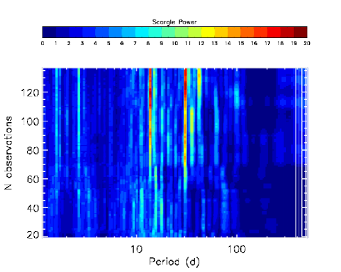
Figure 2: Periodogram power of the inspected periods as a function of the number of observations. The most significant periods (the reddest ones) at 30.7 d and 13.7 d are clearly visible with a high power for N_obs $>$ 60, as well as the period at 2.65 d with a moderate Scargle power, which increases for N_obs $>$ 80 and the period at 42.5 d whose power increases for N_obs $>$ 110 (2D plot adapted from A. Mortier - Private Communication).

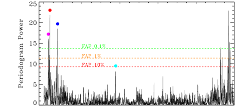
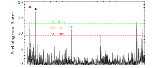
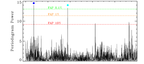
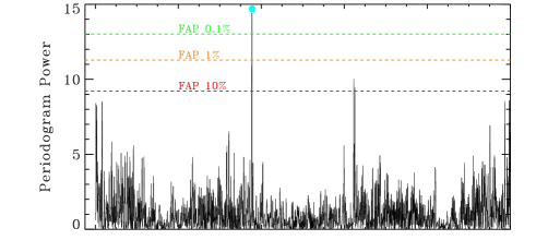
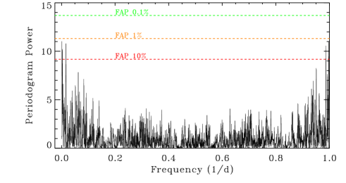
Figure 3: GLS periodograms of the radial velocities of GJ 3998, of the original data (upper panel) and after removing - from top to bottom - the 30.7 d (marked with the red dot), the 42.5 d (magenta dot), the 13.7 d (blue dot) and finally the 2.65 d (cyan dot) signals. The dashed lines indicate 0.1%, 1% and 10% level of false alarm probability.

4 Data analysis

The raw rms dispersion of the RVs is 4.24 m s^-1 which is much higher than the average (Doppler + jitter) uncertainty ¡$\sigma_{i}$¿ $\approx$  1.4 – 2.6 m s^-1, depending on the assumed jitter ($\sigma_{jitter}$ = 0.8 m s^-1, from our first estimate from Gaussian Process, and $\sigma_{jitter}$ = 2.4 m s^-1, following the derivation from Perger et al. 2016 (submitted), respectively). An F-test with F = $\sigma_{e}^{2}/<\sigma_{i}>^{2}$ (Zechmeister & Kürster, 2009) returned a negligible probability ($<10^{-8}$) that the photon noise combined with stellar jitter explains the measured dispersion.

The first step of the RV data analysis consists in identifying significant periodic signals in the data. Prewhitening is a commonly used tool for finding multi-periodic signals in time series data. With this method we find sequentially the dominant Fourier components in a time series and remove them. The prewhitening procedure was applied to the full RV data using the Generalized Lomb-Scargle (GLS) periodogram algorithm (Zechmeister & Kürster, 2009) and the program $\it Period04$ (Lenz & Breger, 2004), to have an independent test. The two methods give the same results in terms of extracted frequencies from our RV time series. Due to the limited range in frequency covered by the found signals, we repeated the analysis by using the iterative sine-wave fitting least-squares method (Vaníček, 1971). This approach is used in the asteroseismic analysis of multiperiodic pulsating stars to minimize the subtle effects of prewhitening, such as power exchange between a signal frequency and an alias of another signal frequency. After each detection, only the frequency values were introduced as known constituents in the new search. In such a way their amplitudes and phases were recalculated for each new trial frequency, always subtracting the exact amount of signal for any known constituent. This new analysis confirmed once more the frequencies previously found.
We calculated the false alarm probabilities (FAP) of detection using 10 000 bootstrap randomization (Endl et al., 2001) of the original RV time series. Once a significant peak was located at a given period, the corresponding sinusoidal function was adjusted and removed. The process was repeated several times until no significant peak remained.
To visualize (Fig. 2) the cumulative contribution of data points to the significance of the detected frequencies, we calculated the GLS periodograms increasing the number of observations, from 20 to 136, adding one observation at a time (following the exact order of data acquisition). We compute the power corresponding to each of the 5000 periods in the range 1.2 d to 500 d, for each of the 117 periodograms obtained. Each horizontal slice of Fig. 2 gives powers (indicated by the color scale) versus periods for the periodogram corresponding to the observations number, indicated on the vertical axis. Fig. 2 is a 2D rapresentation adapted from A. Mortier (Private Communication).

Following this procedure, we identified three frequencies with FAP smaller than 0.1%, at 0.0326 d^-1 (P = 30.7 d), 0.0729 d^-1 (P = 13.7 d) and 0.0235 d^-1 (P = 42.5 d), in order of decreasing power. After removing the sinusoid corresponding to the period of 30.7 d, with a semi-amplitude of 3.4 m s^-1, two highly significant peaks are seen in the periodogram, at 42.5 d and 13.7 d, with semi-amplitudes of 2.5 and 2.1 m s^-1 (Fig. 3). One additional peak remains at 0.3773 d^-1 (P = 2.65 d) with a significant FAP smaller than 0.1% and a semi-amplitude of 1.7 m s^-1. A low frequency signal with a FAP around 1% remains after subtracting the four significant periods. This unresolved peak is probably the signature of a long-term variation of the activity, having a time scale of about 600 d or more. Indeed, this low frequency peak was found in both the activity indicators ($S$ index and H$\alpha$, Sect. 4.1). Moreover, it almost disappears when introducing a linear term in the frequency analysis of the RV time series.
A careful analysis of the spectral window, following the methods of Dawson & Fabrycky (2010), ruled out that the peaks in the periodograms are artifacts due to the combination of the long-term activity with the spectral window (or to the time sampling alone).

4.1 Periodic signals: planet vs activity-related origin

The purely frequentistic approach highlighted the presence of four significant frequencies in the RV time series. However, when dealing with M-type stars we have to face one of the major drawbacks of this kind of stars: many M stars show some level of activity, even if moderate, and display inhomogeneities on their surface that rotate with the star. These inhomogeneities cause RV shifts due to the distortion of the spectral line shape, and these shifts can $\it mimic$, confuse or even hide the planetary signal.

To investigate RV variability against stellar activity, we make use of spectral indices based on Ca II H&K ($S$ index) and H$\alpha$ lines and we take advantage of the photometric observations of the star within the APACHE and EXORAP photometric programs, to check whether plages or spots could produce the observed Doppler changes (Sect. 5).

Table 2: Ca II H & K (top) and H$\alpha$ (bottom) windows.

Band	Center (Å)	Width (Å)
Blue wing	3901.07	20
K core	3933.67	3.28
H core	3968.47	3.28
Red wing	4001.07	20
Blue wing	6550.87	10.75
H$\alpha$  core	6562.81	1.6
Red wing	6580.31	8.75

Stellar activity is usually characterised by the strength of the central cores of the Ca II H & K lines with respect to a reference flux measured at each side of the lines. Activity $S$ indexes are measured by summing the fluxes in the central cores of the Ca II H & K lines and rationing this sum to the sum of fluxes in two 20 Å  windows on either side of the lines. The definition of the windows is done following Henry et al. (1996) (Suárez Mascareño et al., 2015), and it is summarized in Table 2. Fluxes were measured using the IRAF task sbands. Before measuring the fluxes, each individual spectrum was corrected from its corresponding RV by using the IRAF task dopcor. Uncertainties in the $S$ indexes were obtained by shifting the center of the red and blue wings by $\pm$ 0.2 Å. Typical uncertainties vary between 1$\cdot 10^{-3}$ and 5$\cdot 10^{-4}$ (Maldonado et al. 2016, submitted).

H$\alpha$ emission is measured by summing the fluxes in the central core of the line at 6562.808 Å  with a width of 1.6 Å  and rationing this sum to the sum of fluxes in two windows on either side of the line (see Table 2). The H$\alpha$ line at $\lambda$ = 6562.808 Å  is sensitive to the mean chromospheric activity (Kürster et al., 2003; Bonfils et al., 2007; Robertson et al., 2013), as Ca II H & K lines. The RV and activity indices H$\alpha$  and $S$ index measurements of the star GJ 3998 are displayed in Fig. 1 as a function of time.
The analysis of the activity indicators was performed with the GLS algorithm and periodic variations around 30.7 and 42.5 d are indeed observed in the $S$ index and H$\alpha$, whereas no signal appears around 13.7 and 2.65 days, as illustrated in Fig. 4 showing the GLS periodograms of these parameters zoomed around the frequencies of interest.
The outcomes of the activity analysis support the non-planetary origin of the 30.7 d and 42.5 d signals and give us an indication of the stellar rotation period and of a differential rotation, consistently with the outcomes of a recent analysis based on a wide dataset, including M stars, of $Kepler$ time series, as discussed in Sect. 7. This rotation period is consistent with the predicted Prot $\approx$ $34.7\pm 6.9\,d$ from the formula in Suárez Mascareño et al. (2015) according to the log$R^{\prime}_{\mathrm{HK}}$ $\approx$ -5.01.

In order to avoid any misinterpretation of the stellar activity as a planetary signal, we analysed two subsets of the data (before and after BJD-2 457 000.0 d) to check the persistence of the planetary signals over time and to mitigate the possible effects of discontinuities in the data sampling. In Fig. 5 we show the GLS periodograms zoomed around the frequency ranges of interest, black-line for the first subset (61 RV points) and red-line for the second subset (75 RV points). In the plot we indicated the frequencies obtained from the RV (green) and activity indices (blue) analysis and from the photometry (orange) (see Sect. 5). Whilst the periods related to activity effects (related to magnetic phenomena, like spots and faculae, rotating on the stellar surface and the presence of differential rotation) span a range from 28 to 41 d in the two seasons (f = 0.036 d^-1 to f = 0.024 d^-1), the two features at P₁ = 2.65 d (f = 0.3773 d^-1) and P₂ = 13.7 d (f = 0.0729 d^-1) are observed in both seasons. This constitute a further evidence that these two signals are present in the RVs at any time, leading us to the conclusion of a planetary origin for both signals.

Another argument in favour of the planetary interpretation of the 2.65 d and 13.7 d signals is provided in Fig. 6 by the low Spearman’s rank correlation coefficients between the S index ($\rho$ = 0.17) and H$\alpha$ ($\rho$ = 0.18) and the RV residuals after removing the activity contributions (30.7 d and 42.5 d). Such a correlation would be expected if the radial velocity variation is still induced by activity features on the star surface.
The activity indices analysis has been performed with both the values calculated by the TERRA pipeline and those calculated, independently, using the method described above, obtaining the same results.

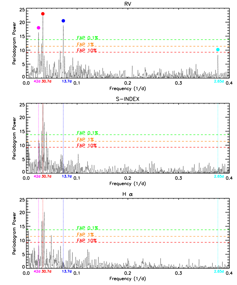
Figure 4: From Top to Bottom the panels show the GLS periodograms of radial velocities, $S$ index and H$\alpha$, zoomed around the frequencies of interest. The dotted blue and cyan lines indicate the frequencies corresponding to orbital periods of the candidate planets at 13.7 d and 2.65 d, respectively, while the dotted red and magenta lines the frequencies corresponding to the activity periods at 30.7 d and 42.5 d, respectively. These frequencies/periods are marked with dots, with the same color code, in the upper RV panel.

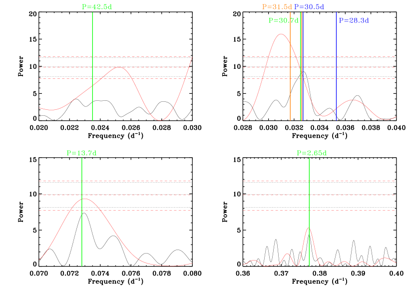
Figure 5: GLS periodograms around the frequency ranges of interest, for two subsets of the original RV data. The first seasons has 61 data points and its periodogram is black (FAP: 0.1%, 1%, 10% horizontal black dotted lines), the second season has 75 data points and is plotted in red (FAP: 0.1%, 1%, 10% horizontal red dashed lines). The two upper panels refer to the frequencies related to activity (f = 0.0235 d^-1 – P = 42.5 d upper left panel; f = 0.0326 d^-1 – P = 30.7 d upper right panel). The two lower panels refer to the frequencies related to the candidate planets (f = 0.0729 d^-1 – P = 13.7 d lower left panel; f = 0.3773 d^-1 – P = 2.65 d lower right panel). The relevant frequencies derived from all the methods used on the full dataset are indicated with vertical lines green from RV analysis, blue from activity indices and orange from photometry (see Sect. 5).

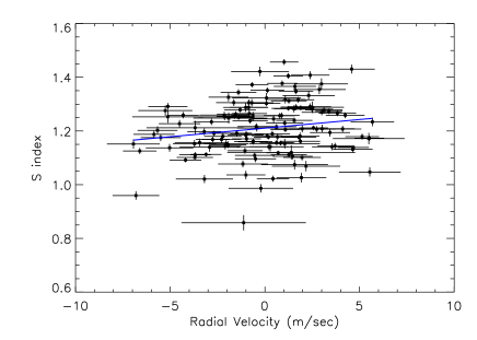
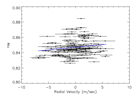
Figure 6: Radial velocity after subtracting the contributions of the activity signals at 30.7 d and 42.5 d, displayed as a function of the $S$ index (top) and H$\alpha$ (bottom). The extremely low correlation values support the planetary interpretation of the 2.65 d and 13.7 d signals still present in the data.

5 Photometry

The targets of the HADES program are photometrically monitored by two independent programs: APACHE and EXORAP.
These two programs regularly follow-up the sample of M stars to provide an estimate of the stellar rotation periods by detecting periodic modulation in the differential light curves.

5.1 EXORAP photometry: dataset

GJ 3998 was monitored at INAF-Catania Astrophysical Observatory with a 80cm f/8 Ritchey-Chretien robotic telescope (APT2) located at Serra la Nave (+14.973^∘E, +37.692^∘N, 1725 m a.s.l.) on Mt. Etna. The APT2 camera is an ASPEN CG230 equipped with a 2k$\times$2k e2v CCD 230-42 detector operated with a binning factor of 2 (pixel scale 0.94$"$) and a set of standard Johnson-Cousins $UBVRI$ filters. The data were reduced by overscan, bias, dark subtraction and flat fielding with the IRAF procedures, and visually inspected for quality checking. We collected $BVRI$ photometry of GJ 3998 in 75 nights between 5 May 2014 and Sept,17 2015. The log of the two observing seasons is given in Table 3. We used aperture photometry as implemented in the IDL routine aper.pro, trying a range of apertures to minimize the rms of the ensemble stars.

To measure the differential photometry, we started with an ensemble of $\sim$6 stars, the nearest and brightest to GJ 3998 and checked the variability of each of them building their differential light curves using the remaining ensemble stars as reference. With this method we selected the least variable stars of the sample, typically 4 of them. The rms of the ensemble stars is $\lesssim 9$ mmag in all bands.

Table 3: EXORAP observations log for GJ 3998

Season	Start	End	Data points
			B	V	R	I
2014	5 May	30 Jul	26	25	24	32
2015	15 Jan	17 Sep	49	50	44	24
All data			75	75	68	56

5.1.1 EXORAP photometry: Searching for periodic variability

The differential photometry of the target is analyzed using the GLS algorithm. We analyzed the full dataset and each season separately (Table 3). No data were rejected after evaluation for outliers (clip at 5$\sigma$). For each band, we analyzed the periodograms, assigning them the FAP using the bootstrap method with 10 000 iterations. The periodograms of the $R$ and $I$ magnitudes do not show any peak above the $10\%$ significance level. The periodogram of the $B$ measurements is affected by a long-term trend: the combination with the spectral window aliasing makes the determination of the periodicities, if any, very difficult. The results obtained from the $V$ measurements are more reliable. We find a good confirmation of the 30.7 d period (P = $30.75\pm 0.12\,d$, the precision is the formal error from the least square fitting), though flanked by the aliases at $\pm$1 cycle/year To check for possible systematic effects, we repeated the search for periodicity on all the measured stars in the field of view of GJ 3998 (about 70 targets), but none of them shows significant variability with the same periodicity of our target star.

The photometric period is consistent with the one found by the analysis of variability of features sensitive to stellar activity in the HARPS-N data (Sect. 4.1). The $V$ light curve folded with the observed periodicity is shown in Figure 7 (the $B$ light curve folded with the same periodicity is also shown). It shows a full amplitude of 0.012 mag. We note that the observed variability amplitude in the $V$ band is typical for an M2 dwarf as shown by Rockenfeller et al. (2006), who also report variability amplitudes in the $R$ and $I$ bands that are about half that of the $V$ band. With a precision of a few millimag, a signal with a five-millimag full-amplitude only remains elusive to us, hence the lack of period detection in the $R$ and $I$ data.

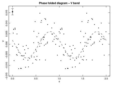
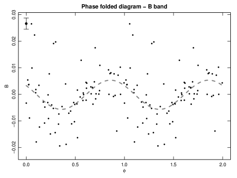
Figure 7: Phase folded V and B curves at the periods P = $30.75\pm 0.12\,d$, the precision reported is the formal error from the least square fitting.

5.2 APACHE photometry: dataset

APACHE is a photometric survey devised to detect transiting planets around hundreds of early-to-mid M dwarfs (Sozzetti et al., 2013). GJ 3998 was monitored for 41 nights between June 30, 2014, and August 13, 2015, with one of the five 40cm telescopes composing the APACHE array, located at the Astronomical Observatory of the Autonomous Region of the Aosta Valley (OAVdA, +45.7895 N, +7.478 E, 1650 m.a.s.l.). Each telescope is a Carbon Truss f/8.4 Ritchey-Chretien equipped with a GM2000 10-MICRON mount and a FLI Proline PL1001E-2 CCD Camera, with a pixel scale of 1.5 ^′′/pixel and a field of view of 26^′x26^′. The observations were carried out using a Johnson-Cousins V filter following the standard strategy used by APACHE, consisting in three consecutive exposures repeated at intervals of $\sim$20-25 minutes, while the target is $\sim 35^{\circ}$ above the horizon. The images were reduced with the standard pipeline TEEPEE written in IDL by the APACHE team (see Giacobbe et al., 2012). TEEPEE is devised to perform ensemble differential aperture photometry by testing up to 12 different apertures and choosing the best set of comparison stars that give the smallest rms for the differential light curve of the target.

5.2.1 APACHE photometry: Analysis of the light curves

The APACHE data were obtained by using an aperture of 4.5 pixel and a set of 4 comparison stars (UCAC4 506-065211, UCAC4 506-065134, UCAC4 505-066479, and UCAC4 506-065155). The stellar brightness decreases almost linearly during the second season (Spearman’s rank correlation coefficient $\rho=-0.66$, computed with the r$\_$correlate IDL function), and the $\sim$6 mmag rms of the data, which is comparable to the typical photometric precision of the measurements, is not indicative of high photospheric variability. The brightness decrease is not confirmed by the EXORAP $V$ photometry and hence its origin remains unclear. We searched the light curve for sinusoidal-like modulation by using the complete dataset consisting of 455 points, each being the average of three consecutive measurements with uncertainty equal to their rms. We used the GLS and $\it Period04$ algorithms to calculate the frequency periodograms. Gaps in the data and in the folded light curves make a little uncertain the accurate identification of the true period around 30-35 d. The analysis performed with $\it Period04$ returned a maximum frequency corresponding to a period of about 31.5 d, in good agreement with the results of the EXORAP photometry, while the GLS analysis returned the 1 cycle/year alias at 34.5 d. The best-fit semi-amplitude of the sinusoid is $\sim 5$ mmag. Fig. 8 shows the light curve folded at the best period found. To estimate the significance of the detection, we performed a bootstrap analysis (with replacement) by using 10 000 fake datasets derived from the original photometric data, and found a FAP $\leq$ 1.0$\%$. While indicating a rather significant detection, this result should be taken with caution because the signal semi-amplitude is close to the typical precision of the data. However, it is noteworthy that the best photometric frequency we find is close to that found in the RVs and spectroscopic activity index time series, which we explained as related to the stellar rotation frequency. In sight of this, we conclude that the APACHE photometry further supports the interpretation based on spectroscopic evidence. We searched the light curve also for possible transit-like signals of the candidate planets, but none was detected. However, this search is not conclusive since the number of observations and the photometric precision are too low to rule out signals in this period domain.

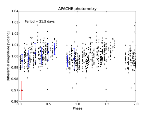
Figure 8: Differential light curve of GJ 3998 observed by APACHE, folded at the best period P=31.5 days found through a frequency analysis of the time series. The red dot in the lower left corner is to show the average uncertainty of the data.

5.3 FastCam Lucky Imaging Observations

On October 1st 2014 at 22:04 UT, we collected 50,000 individual frames of GJ3998 in the I band using the lucky imaging FastCam instrument (Oscoz et al., 2008) at the 1.5m Carlos Sánchez Telescope (TCS) at the Observatorio del Teide, Tenerife, with 30 ms exposure time for each frame. FastCam is an optical imager with a low noise EMCCD camera which allows to obtain speckle-featuring not saturated images at a fast frame rate, see Labadie et al. (2011).

In order to construct a high resolution, diffraction limited, long-exposure image, the individual frames were bias subtracted, aligned and co-added using our own Lucky Imaging (LI) algorithm, see Law et al. (2006). Fig. 9 presents the high resolution image constructed by co-addition of the 20% of the best frames, resulting in a total integration time of 300 seconds. The combined image achieved $\Delta m_{I}=2.5-3.0$ at $1\aas@@fstack{\prime\prime}0$, finding no bright contaminant star in the diffraction limited image.

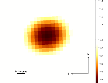
Figure 9: Diffraction-limited image of GJ3998 after lucky imaging processing with a 20% selection of the best individual TCS/FastCam frames.

6 MCMC analysis of the radial velocity time series

To derive the system parameters with the associated uncertainties and also to double check the purely frequentist approach, we performed a Bayesian analysis of the RV data by using the publicly available emcee tool (Foreman-Mackey et al., 2013), a Python implementation of the Affine Invariant Markov chain Monte Carlo (MCMC) Ensemble sampler. Under the hypothesis that up to four significant signals exist in the data (i.e. two of planetary origin and two ascribable to the stellar activity), as inferred from the analysis described in Sect. 4.1, we tested several different models by changing the number of planets, assuming circular or eccentric orbits for the outer planet, and examining different ways to model the stellar activity noise. In all the cases we included an additional ’jitter’ term summed in quadrature with the RV uncertainties. We used uniform priors for all the fitted parameters, by keeping unchanged their range of variability when passing from one model to the other. The best fit values are calculated as medians of the marginal posterior distributions, and the uncertainties represent their 16$\%$ and 84$\%$ quantiles. In modelling the RVs we ignored the mutual gravitational perturbations between the two planets.

6.1 Modelling the stellar activity noise

The comparative analysis of the periodograms for the $S$ activity index and RVs, also supported by photometry, showed in the data a clear existence of a nearly periodic noise term of stellar origin, whose recurrence is likely ascribable to the stellar rotation. We take this evidence into account in our RV analysis by treating the short-term activity (i.e. related to the stellar rotation) in two different ways.

As a first trial, we considered a strictly periodic term by fitting a sinusoid with period constrained between 25 and 45 days. Additionally, we used PyORBIT (Malavolta et al., 2016) to test several combinations of sinusoids at the stellar rotational period and its harmonics, and independent amplitudes and phases for each observing season, without observing a significant improvement with respect to a single sinusoid approach.

As a second, more sophisticated trial we treated the stellar activity term as correlated quasi-periodic noise, by using the approach based on Gaussian Processes (GPs; see, e.g. Rasmussen & Williams 2006 and Roberts et al. 2012). In this case the stellar noise is conveniently described by means of a covariance function, opportunely selected, whose functional form and parameters have some correspondence to the physical phenomena to be modelled. The GP framework can thus be used to characterize the activity signal without requiring a detailed knowledge, for instance, of the distribution of the active regions on the stellar surface, their lifetime or their temperature contrast, which is almost always inaccessible.

To model the short-term activity in the GP framework we used the publicly available GEORGE Python library for GP regression (Ambikasaran et al., 2014), and adopted the quasi-periodic kernel described by the covariance matrix

$$k(t,t^{\prime})=h^{2}\cdot\exp\large[-\frac{(t-t^{\prime})^{2}}{2\lambda^{2}}-\frac{sin^{2}(\pi(t-t^{\prime})/\theta)}{2w^{2}}\large]+$$

$$+\,(\sigma^{2}_{RV}(t)\,+\,\sigma_{j}^{2})\cdot\delta_{t,t^{\prime}}$$ (1)

where $t$ and $t^{\prime}$ indicate two different epochs. This kernel has been used with profit in several recent works on exoplanets to mitigate the impact of the stellar noise in the RV data (see, e.g., Haywood et al., 2014; Grunblatt et al., 2015; Faria et al., 2016; Mortier et al., 2016), because its functional form encompasses some properties of stellar activity that we can reasonably conceive. In fact, being composed by a periodic term coupled to an exponential decay term, this kernel describes a recurrent signal linked to the stellar rotation, and takes into account for a finite lifetime of the active regions and evolution of their size. The parameters of the covariance function (also called hyper parameters) can be interpreted as follows:

• $h$ represents the amplitude of the correlations;

• $\theta$ is usually related to the rotation period of the star (or one of its harmonics);

• $w$ is the length scale of the periodic component, and can be linked to the size evolution of the active regions;

• $\lambda$ is the correlation decay timescale, and it can be related to the lifetime of the active regions.

Equation (6.1) also includes a term with the uncorrelated noise, added quadratically to the diagonal of the covariance matrix. Here, $\sigma_{\rm RV}(t)$ is the RV uncertainty at time t, $\sigma_{j}$ is the additional noise we fit in our models to take into account instrumental effects and other $\lesssim 1\hbox{\,m\,s${}^{-1}$}$ noise sources not included in the internal errors and in our stellar activity framework, and $\delta_{t,t^{\prime}}$ is the Dirac delta function.

Despite the activity index datasets suggest the existence of a long-term trend (i.e. hundreds of days), with properties that are far to be constrained by our data (see Sect. 4), the radial velocity time series shows a very weak similar trend, and for this reason we decided not to include it in our general RV model.

In the GP framework, the log-likelihood function to be maximised by the MCMC procedure is

$$\ln\mathcal{L}=-\frac{n}{2}\ln(2\pi)-\frac{1}{2}\ln(det\,\mathbf{K})-\frac{1}{2}\overline{r}^{T}\cdot\mathbf{K}^{-1}\cdot\overline{r}$$ (2)

where $n$ is the number of the data points, K is the covariance matrix built from the covariance function in Equation (6.1), and $\overline{r}$ represent the RV residuals, obtained by subtracting the offset and the Keplerian(s) signal(s) (i.e. the ”deterministic” component) to the original RV dataset.

A general form for the different models that we tested in this work is given by the equation

$$\Delta RV(t)=\gamma+\sum_{j=1}^{n_{planet}}\Delta RV_{Kep,j}(t)+$$

$$+\,\Delta RV(t)_{\rm(activity,\,short-term)}$$

$$=\gamma+\sum_{j=1}^{n_{planet}}K_{j}\large[\cos(\nu_{j}(t,e_{j},T_{0j},\textit{P}_{j})+\omega_{j})+e_{j}\cos(\omega_{j})\large]+$$

$$+\,GP\,\LARGE(\mathbf{or}\,A\cdot\sin\large[\dfrac{2\pi\,t}{P_{rot,*}}+\phi]\large\LARGE)$$ (3)

where $n_{planet}=1,2$, $\gamma$ is the RV offset, $P_{\rm rot,*}$ is the stellar rotation period. Instead of fitting the eccentricity $e_{j}$ and the argument of periapsis $\omega_{j}$ separately, we introduce the parameters $C_{j}=\sqrt{e_{j}}\cdot\cos\omega_{j}$ and $S_{j}=\sqrt{e_{j}}\cdot\sin\omega_{j}$ to reduce the covariance between $e_{j}$ and $\omega_{j}$ (Ford, 2006).

The choice in our analysis of the covariance function in Eq. (6.1) appears appropriate by looking at the results obtained from a GP analysis of the $S$ index time series. Here the ”deterministic” component is the mean of the $S$ index. The best fit values of the hyper parameters are showed in Tab. 4. For $\theta$ we find a value which is in good agreement with the stellar rotation period previously estimated, and the value for $\lambda$ appears physically plausible for a Main Sequence star, because it indicates an evolutionary time scale of $\sim$1 month for the active regions, i.e. comparable to the stellar rotation period. Thus, the quasi-periodic kernel in Eq. (6.1) describes reliably the short-term stellar activity pattern imprinted in the $S$ index.

For the MCMC analysis of the RVs, for each model we used 80 random walkers to explore the parameter space, with the GP hyperparameters $w$, $\lambda$, and $\theta$ randomly initialized from normal distributed values around the best estimates summarized in Tab. 4, using their uncertainties as $\sigma$ of the distributions. Same for the guess values of the planetary parameters $K$ and $P$, for which we used the estimates found through the preliminary periodogram analysis, while $T_{\rm 0,conj}$ was initialized to an intermediate value in the prior range we defined. We applied an initial burn-in by definitively removing the first 3,000 steps from each chain. After the selection of the best model, based upon the estimates of the Bayesian evidences (see below), we performed an additional burn-in to derive the parameter estimates by removing from the full list of the posterior samples those having a $\ln\mathcal{L}$ lower than the median of the whole $\ln\mathcal{L}$ dataset. Typically, the convergence of the MCMC chains has been reached after $\sim$35,000 steps of the random walkers, with parameter correlation lengths $\sim$1,000-2,000.

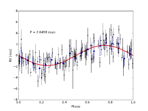
Figure 10: RV data folded at the best-fit orbital period of the inner planet. The signal of the outer planet, the RV offset and the best-fit GP solution for the stellar activity noise have been subtracted. Blue dots are the mean values in bins of amplitude 0.05. The red solid line is the best-fit orbital solution.

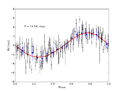
Figure 11: RV data folded at the best-fit orbital period of the outer planet. The signal of the inner planet, the RV offset and the best-fit GP solution for the stellar activity noise have been subtracted. Blue dots are the mean values in bins of amplitude 0.05. The red solid line is the best-fit orbital solution.

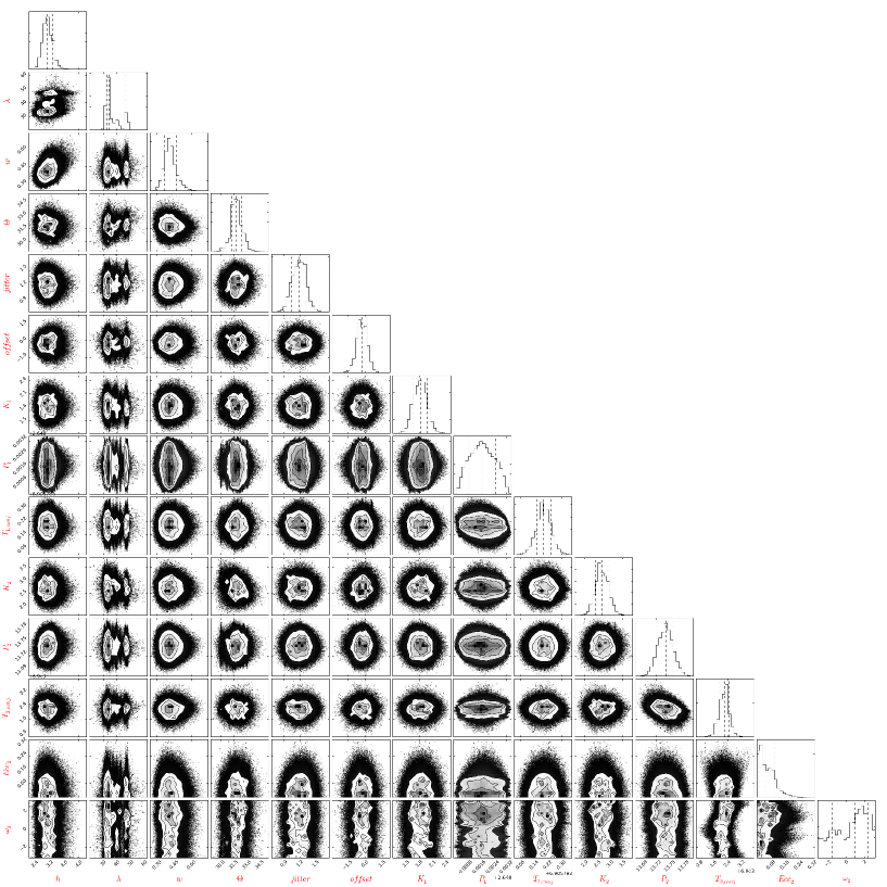
Figure 12: Marginal posterior distributions for the parameters of our model, which include two Keplerians and a GP-based fit for the short-term stellar noise. Vertical dashed lines indicate the median values and the 16$\%$ and 84$\%$ quantiles of the distributions.

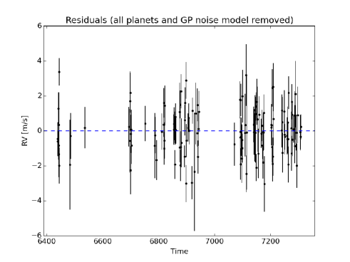
Figure 13: Residuals of the global fit (activity+Keplerians) we used to model the RV data set.

6.2 Model selection and planetary parameters

Following the principles of Bayesian inference, for each of the tested models we calculated the logarithm of the Bayesian evidence $\mathcal{Z}$ to perform a model comparison and selection. To this purpose, because the estimate of $\mathcal{Z}$ is notoriously a challenging numerical task, we used two different estimators proposed in literature (Chib & Jeliazkov 2001, hereafter C$\&$J estimator; and Perrakis & Tsionas 2014, hereafter Perr estimator). For the interpretation of the model probabilities we follow here a conventional empirical scale often used (a slightly modified version of the so-called ”Jeffreys’ scale”), which states that the model with the highest $\mathcal{Z}$ is strongly favoured over the other when $\Delta\ln\mathcal{Z}\geqslant 5$, while $2.5<\Delta\ln\mathcal{Z}<5$ denotes moderate evidence, $1<\Delta\ln\mathcal{Z}<2.5$ weak evidence, and $\Delta\ln\mathcal{Z}<1$ corresponds to inconclusive evidence.

We report in Tab. 5 only the Bayesian evidences $\ln\mathcal{Z}$ for the models involving two Keplerian signals, which will be the object of our discussion. In fact, as expected from our previous analyses, models involving only one planet appear much less probable than those with two planets, independently on the framework used to account for the stellar activity. For instance, for circular orbits and considering only the C$\&$J estimator, $\Delta\ln\mathcal{Z}\sim 17$ between the 2-planet model and that with only the outer companion, $\Delta\ln\mathcal{Z}\sim 5$ when the model with only the inner planet is considered.

In Tab. 6 we summarize the results for the final model we selected. The short-term stellar activity is modelled better in the GP framework with respect to a sinusoid. For instance, for 2-planet circular models the C$\&$J estimator results in $\Delta\ln\mathcal{Z}=\ln\mathcal{Z}_{\rm GP}-\ln\mathcal{Z}_{\rm sin}\sim 16$. The reason probably lies in the lifetime of the active regions $\lambda$, which is too short to be properly modelled by a strictly periodic function.

We adopt here the model with the eccentricity of the outer planet treated as a free parameter (model number 3 in Tab. 5). According to the statistical evidence, it is as likely as the simpler model with circular orbits (number 2), but we select it for convenience despite it involves a greater number of free parameters. In fact, by adopting model 3 we provide an upper limit on the outer planet eccentricity that can be useful for statistical studies, despite our estimate of $e$ is indicative of a circular orbit. For completeness, we also tested the model where the eccentricities of both planets are treated as free parameters (model 4 in Tab. 5). Based on a simple tidal dissipation model, we expect that the orbital eccentricity of the inner planet should be negligible. In fact, if the modified tidal quality factor of the inner likely super-Earth planet $Q^{\prime}\sim 1400$, i.e., similar to that of the Earth in the case of the semidiurnal tide raised by the Moon (Lainey, 2016), and the outer planet does not significantly excite the eccentricity of its orbit, the tidal dissipation inside the inner planet can circularize its orbit with an e-folding timescale of only $\sim 65$ Myr, i.e., much shorter than the likely age of the system, as we can reasonably deduce from the quite long stellar rotation period. Our analysis results in $e=0.36^{+0.10}_{-0.12}$ for the eccentricity of planet $b$, and $e=0.061^{+0.059}_{-0.039}$ for that of planet $c$ (16$\%$ and 84$\%$ quantiles), with a Bayesian evidence which is slightly worse or slightly better than model 3, depending on the estimator (Tab. 5). Thus, there is at most only a weak statistical evidence to prefer model 4 over model 3, with the latter that has fewer free parameters and therefore it is adopted also because simpler. In Figs. 10 and 11 we show the RV data folded at the best-fit orbital period of the inner and outer planets, respectively, as well as the best-fit orbital solution. In each plot the signal of the other planet, the RV offset and the best-fit GP solution for the stellar activity noise have been subtracted. In Fig. 12 we show the marginal posterior distributions for the parameters of the selected model. The RV residuals are showed in Fig. 13. No residual long-term trend is visible in the data, supporting our a-priori decision of not including an additional term to model a possible stellar activity cycle. The analysis of the residuals with the GLS algorithm does not show any significant periodicity left in the data, meaning that the GP has absorbed the signal at $\sim 42$ days. This could be related to the best-fit value assumed by the $\lambda$ time scale. In fact, the upper uncertainty on $\lambda$ is quite high ($\sim 11$ days) and this is related to the presence of a secondary peak visible in the marginal posterior distribution for $\lambda$ slightly higher than 40 days.

When looking at the best-fit values of the covariance function hyper parameters, that are showed in Tab. 6, we note that the distributions of $\lambda$ and $\theta$, which was constrained within a range that includes the two ’activity’ periods found through the periodogram analysis, appear quite similar to those for the $S$ index. Because of their physical interpretation, one can expect them to remain almost unchanged when passing from the $S$ index to the RVs if the structure of the correlated (stellar) noise is similar in both data sets. Moreover, both for the $S$ index and RVs $\theta$ finely settles to a value which is compatible with the estimates of the stellar rotation period previously derived. Thus, there is a convincing evidence that the use of a GP efficiently mitigate the short-term activity noise present in the RV data, resulting in reliable estimates for the orbital and physical parameters of the planets.

Table 4: Best fit values for the hyper parameters of the covariance function in Eq. 6.1, derived from a GP analysis of the $S$ activity index time series using 100 random walkers. They are calculated as medians of the marginal posterior distributions, and the uncertainties represent their 16$\%$ and 84$\%$ quantiles. The priors used in our MCMC fitting are also showed.

Hyper parameter	Value	Prior
$\lambda$ [days]	$30.9\pm 4.9$	$\mathcal{U}$(0,+$\infty$)
$w$	$0.099\pm 0.011$	$\mathcal{U}$(0,+$\infty$)
$\theta$ [days]	$29.2\pm 0.19$	$\mathcal{U}$(25,50)

Table 5: Summary of the Bayesian statistical evidences $\ln\mathcal{Z}$ for the two-planet models tested in this work. References to the three different methods used are given in the text.

Model nr.	Nr. of free param.	Eccentric/circular orbit	Stellar activity model	$\ln\mathcal{Z}_{C\&J}$	$\ln\mathcal{Z}_{Perr}$
1	11	c+c	Sinusoid + jitter	-332.5	-340.4
2	12	c+c	GP + jitter	-316.8	-316.7
3	14	c+e	GP + jitter	-314.2	-315.5
4	16	e+e	GP + jitter	-315.4	-313.6

Table 6: Best-fit values for the parameters of the global model (two planets + stellar activity) selected as explained in 6.2. They are calculated as medians of the marginal posterior distributions, and the uncertainties represent their 16$\%$ and 84$\%$ quantiles, unless otherwise indicated. The priors used in our MCMC fitting are also showed.

Parameter	Value	Prior
(planets)
Planet $b$
$K$ [ m s-1]	$1.82^{+0.14}_{-0.16}$	$\mathcal{U}$(0,$+\infty$)
$P$ [days]	$2.64977^{+0.00081}_{-0.00077}$	$\mathcal{U}$(1.5, 3.5)
$T_{\rm 0,conj.}$ [BJD-$2,450,000$]	$6905.895^{+0.042}_{-0.040}$	$\mathcal{U}$(6900, 6915)
$e$	0 (fixed)	-
$a$ [au]	$0.029\pm 0.001$	derived
$m_{\rm p}\hbox{sin\,$i$}$ [$M_{\oplus}$]	$2.47\pm 0.27$	derived
Planet $c$
$K$ [ m s-1]	$2.67^{+0.28}_{-0.23}$	$\mathcal{U}$(0,$+\infty$)
$P$ [days]	$13.740\pm 0.016$	$\mathcal{U}$(12, 15.5)
$T_{\rm 0,conj.}$ [BJD-$2,450,000$]	$6902.2^{+0.24}_{-0.29}$	$\mathcal{U}$(6900, 6915)
$e$	$0.049^{+0.052}_{-0.034}$
	$0.049^{+0.094}_{-0.045}$ ($5\%$  and  $95\%$ quantiles)
$\omega$ [rad]	unconstrained
$\sqrt{e}\cdot\sin\omega$	$0.079^{+0.17}_{-0.21}$	$\mathcal{U}$(-1, 1)
$\sqrt{e}\cdot\cos\omega$	$-0.003^{+0.161}_{-0.155}$	$\mathcal{U}$(-1, 1)
$a$ [au]	$0.089\pm 0.003$	derived
$m_{\rm p}\hbox{sin\,$i$}$ [$M_{\oplus}$]	$6.26^{+0.79}_{-0.76}$	derived
$RV_{\rm offset}$ [ m s-1]	$-0.27^{+0.49}_{-0.43}$	$\mathcal{U}$(-5, +5)
(hyper)Parameter	Value	Prior
(stellar activity)
$h$ [ m s-1]	$3.07^{+0.29}_{-0.24}$	$\mathcal{U}$(0,$+\infty$)
$\lambda$ [days]	$34.4^{+11.6}_{-2.0}$	$\mathcal{U}$(0,$+\infty$)
$w$	$0.41^{+0.05}_{-0.04}$	$\mathcal{U}$(0,$+\infty$)
$\theta$ [days]	$31.8^{+0.6}_{-0.5}$	$\mathcal{U}$($25,45$)
$\sigma_{jitter}$ [ m s-1]	$1.19^{+0.11}_{-0.14}$	$\mathcal{U}$($0,20$)

7 Discussion and conclusions

We have presented in this paper the first results from the HADES programme conducted with HARPS-N at TNG. We have found a planetary system with two super-Earths hosted by the M1 dwarf GJ 3998, by analysing the high precision, high resolution RV measurements in conjunction with almost-simultaneous photometric observations. We based our analysis on RV measurements obtained with the TERRA pipeline, which enables us to circumvent potential mismatch of the spectral lines that may happen using a CCF technique for M stars. The homogeneous analysis of the RV observations was carried out both with a frequentistic approach and by comparing models with a varying number of Keplerian signals and different models of the stellar activity noise. The analysis of the radial velocity time series unveiled the presence of at least four significant periodic signals, two of these are linked to the activity of the host star and two to orbital periods:

• P = 30.7 d, gives us an estimate of the rotational period of the star;

• P = 42.5 d, could be indicative of a modulation of the stellar variability due to differential rotation;

• P = 2.6 d, orbital period of GJ 3998b;

• P = 13.7 d, orbital period of GJ 3998c.

The conclusions on activity-related periods are confirmed by the analyses of the activity indicators and of the photometric light curves of two independent sets of observations. The time series of $S$ index and H$\alpha$ show periodic variations around the 30.7 d and 42.5 d signals. The photometric results from both programs confirm the presence of variations in the period range 30 d – 32 d, highlighting the strong connection of the long RV periods to chromospheric activity and to its rotational modulation. Due to its smaller amplitude and effect than the period of 30.7 d, the periodicity at 42.5 d could not be detected in the photometric time series, having a time coverage worst than that of the spectroscopic ones, too. For the same reason, the search for any robust correlation like $BV$ photometry vs. H$\alpha$ or $S$ indexes is unfortunately inconclusive.
Our results show that the detection of small planets in these data could be hampered by activity-induced signals. As a target of the HADES programme, GJ 3998 is included in several statistical studies with the aim to scrutinize in deep the activity properties and rotations of M-dwarfs (Perger et al. 2016, submitted, Maldonado et al. 2016, submitted, Suárez Mascareño et al., Scandariato et al., in preparation). In particular, the accurate analysis of activity indicators performed by Suárez Mascareño et al. (in preparation), including also 6 HARPS (ESO) observations of GJ 3998 acquired more than five years before the start of the HADES programme, provides an estimate of $30.8\,\pm 2.5\,d$ for the rotational period and the hint of an activity cycle 500-600 d long.
In general, differential rotation is not yet fully understood, see e.g. the discussion in Küker & Rüdiger (2011), therefore empirical data are then preferable. Reiners & Schmitt (2003) made an analysis of solar-type stars using an analysis of the shape of the lines in the Fourier domain. They considered a calibration of the ratio between the positions of the two first zeros of the power spectrum of the line profile as a function of the ratio $\alpha$ between equatorial and polar rotation rate. They obtained an anticorrelation between differential rotation and equatorial velocity: differential rotation is mostly evident in slow rotators. Since GJ3998 is indeed a slow rotator, this might be indeed the case. However, Reiners & Schmitt only considered solar-type stars and they do not show that we could see such trends in time-series of M dwarfs.

The most relevant data for us are then those provided by the analysis of the exquisitely sensitive time series obtained with Kepler. Using Kepler data, Reinhold & Gizon (2015) analysed an extremely wide datasets of stars ranging from solar-type stars to M-dwarfs and confirmed the relation found by Reiners & Schmitt between differential rotation and period. We may directly compare our result for GJ 3998 with Figure 9 of Reinhold & Gizon, where they plotted the minimum rotation period (that in our case is 30.7 d), with the parameter $\alpha$=(Pmax-Pmin)/Pmax. For GJ 3998, $\alpha$=(42.5-30.7)/42.5=0.277. The point for GJ 3998 falls exactly in the middle of the points for the M-stars. We would conclude that the assumption that the two periods related to activity for GJ 3998 are due to rotation is fully consistent with what we know about differential rotation.

We run an MCMC simulation and use Bayesian model selection to determine the number of planets in the system and estimate their orbital parameters and minimum masses. We test several different models, varying the number of planets, eccentricity and treatment of stellar activity noise. We select a model involving two Keplerian signals, with a circular orbit for the inner planet and the eccentricity of the outer planet treated as a free parameter. The short-term stellar activity is modelled with the Gaussian Processes approach and the long-term activity noise is not included.

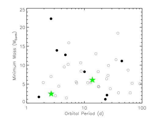
Figure 14: Minimum mass vs. orbital period diagram for known Neptune-type and Super Earth planets around M dwarfs (http://www.exoplanet.eu - black dots, 2016 June 17), the green stars indicate GJ 3998b and GJ 3998c. Filled dots indicate planets with known radius.

The two planets appear to have minimum masses compatible with those of super-Earths, the inner planet has a minimum mass of $2.47\pm\,0.27$  M_⊕, at a distance of 0.029 AU from the host star, the outer has a minimum mass of $6.26^{+0.79}_{-0.76}$  M_⊕ and a semi-major axis of 0.089 AU.
A very rough estimate of the equilibrium temperatures of the planets, from the Stefan–Boltzmann law assuming uniform equilibrium temperature over the entire planet and zero albedo, gives T_eq = 740 K for the inner, and T_eq = 420 K, for the outer planet.
These close distances strongly call for a search of potential transits in the next months, in particular for the inner planet, through a proposal for observing time on the $\it Spitzer\,Space\,Telescope$. This planet has an interestingly high geometric transit probability of $\approx$ 8%. With a minimal mass of $2.47\pm\,0.27$  M_⊕, GJ 3998b’s radius should most likely lie somewhere between $\approx$  1 M_⊕ (metal-rich composition) and $\approx$  1.65 M_⊕ (ice-rich composition) (Seager et al., 2007). Given its host star’s radius of $\approx$  0.5 R_⊙, this range of planetary sizes correspond to plausible transit dephts between 325 to 935 ppm. We thus proposed to use 20hr of $\it Spitzer$ time to monitor a 2-$\sigma$ transit window of the innermost planet in the GJ 3998 system (P.I. M. Gillon). A potential transit could provide a constraining point in the mass-radius diagram of known planets, enabling also the determination of the mean density and a better characterization of the system architecture with future follow-up observations. In particular, there is currently no object with an accurately measured mass ($\leq$ 20%) in the range 2 – 3 M_⊕. This mass gap is even larger if we consider only M dwarf planets, as is evident in Fig. 14, which shows the minimum mass vs. orbital period diagram for known Neptune-type and Super Earth planets around main sequence M stars, along with the location of GJ 3998 planets. The eventuality of a transit, given the small distance from the host and the brightness of GJ 3998 (V = 10.83), would make this star a natural target for follow-up observations with the ESA $CHEOPS$ space telescope and also one of the most interesting M-dwarf targets for a detailed atmospheric characterization.

Appendix A Observing log for the GJ 3998 spectra and results

In this section we report the observing log for the GJ 3998 spectra and the RVs, S and H$\alpha$ indices we obtained with the present study. We list the observation dates (barycentric Julian date or BJD), the signal-to-noise ratios (S/Ns), the radial velocities (RVs) from the DRS and TERRA pipelines and the H$\alpha$ and $S$ indexes, calculated by the TERRA pipeline and in the present study. The RV errors reported are the formal ones, not including the jitter term. The $S$ index and H$\alpha$ errors are calculated as described in the text and do not take into account the photon noise (Sect. 4.1). The $S$ index and H$\alpha$ errors derived from the TERRA pipeline are due to photon noise through error propagation.

Table 7: Data of 136 observed HARPS-N spectra of GJ 3998. We list RVs obtained using the DRS and TERRA pipelines, $S$ index and H$\alpha$ calculated by the TERRA pipeline (indicated with a ’T’) and those derived in the present work, with an independent method.

BJD-2456000	S/N	RV TERRA	RV DRS	$S$ index(T)	H$\alpha$ index(T)	$S$ index	H$\alpha$  index
(d)		(ms-1)	(ms-1)
439.55832	54.1	-3.661$\pm$0.959	-44810.390$\pm$1.403	1.1013$\pm$0.0087	0.8357$\pm$0.0111	0.1025$\pm$0.0003	0.0591$\pm$0.0002
439.65014	54.9	-4.089$\pm$0.839	-44810.869$\pm$1.372	1.0918$\pm$0.0085	0.8366$\pm$0.0106	0.0991$\pm$0.0004	0.0592$\pm$0.0001
441.56648	56.9	3.221$\pm$0.945	-44805.754$\pm$1.317	1.1114$\pm$0.0083	0.8370$\pm$0.0098	0.1026$\pm$0.0002	0.0593$\pm$0.0001
442.54349	62.7	-0.153$\pm$0.819	-44806.802$\pm$1.185	1.1127$\pm$0.0075	0.8367$\pm$0.0086	0.1016$\pm$0.0003	0.0591$\pm$0.0001
443.53644	36.0	2.606$\pm$1.316	-44800.675$\pm$2.070	1.0772$\pm$0.0126	0.8348$\pm$0.0143	0.0982$\pm$0.0002	0.0589$\pm$0.0001
443.63985	25.2	4.881$\pm$1.860	-44797.699$\pm$2.907	1.1528$\pm$0.0179	0.8366$\pm$0.0183	0.1066$\pm$0.0007	0.0591$\pm$0.0001
444.49963	54.4	9.699$\pm$0.779	-44794.175$\pm$1.375	1.1731$\pm$0.0091	0.8348$\pm$0.0099	0.1050$\pm$0.0002	0.0589$\pm$0.0001
444.72822	45.1	3.672$\pm$1.040	-44803.153$\pm$1.659	1.1090$\pm$0.0106	0.8326$\pm$0.0118	0.1023$\pm$0.0003	0.0587$\pm$0.0001
483.60939	18.3	-2.992$\pm$2.562	-44805.750$\pm$4.157	1.2120$\pm$0.0258	0.8477$\pm$0.0249	0.1046$\pm$0.0003	0.0595$\pm$0.0001
485.59901	40.5	-2.053$\pm$1.313	-44810.630$\pm$1.823	1.2590$\pm$0.0129	0.8427$\pm$0.0117	0.1143$\pm$0.0004	0.0594$\pm$0.0001
536.50393	43.7	-0.322$\pm$1.182	-44809.067$\pm$1.696	1.1779$\pm$0.0122	0.8610$\pm$0.0107	0.1110$\pm$0.0003	0.0605$\pm$0.0001
693.77578	37.3	6.167$\pm$1.136	-44800.357$\pm$1.907	1.2448$\pm$0.0138	0.8405$\pm$0.0116	0.1109$\pm$0.0001	0.0598$\pm$0.0001
696.78604	27.5	0.727$\pm$1.817	-44805.115$\pm$2.626	1.3229$\pm$0.0184	0.8442$\pm$0.0160	0.1205$\pm$0.0007	0.0600$\pm$0.0001
697.76988	34.2	1.860$\pm$1.722	-44806.957$\pm$2.162	1.2084$\pm$0.0148	0.8404$\pm$0.0139	0.1120$\pm$0.0005	0.0598$\pm$0.0001
698.75906	31.5	2.978$\pm$1.142	-44808.249$\pm$2.357	1.2340$\pm$0.0160	0.8368$\pm$0.0153	0.1186$\pm$0.0003	0.0593$\pm$0.0001
699.73995	43.7	-5.962$\pm$1.379	-44816.402$\pm$1.667	1.2525$\pm$0.0123	0.8440$\pm$0.0107	0.1165$\pm$0.0002	0.0601$\pm$0.0001
700.76184	48.7	-2.033$\pm$1.096	-44810.392$\pm$1.561	1.2810$\pm$0.0111	0.8452$\pm$0.0114	0.1147$\pm$0.0003	0.0603$\pm$0.0001
701.72684	43.4	-2.388$\pm$1.113	-44811.385$\pm$1.705	1.2905$\pm$0.0121	0.8591$\pm$0.0113	0.1143$\pm$0.0003	0.0613$\pm$0.0001
702.74632	38.5	-5.141$\pm$1.050	-44813.856$\pm$1.816	1.2109$\pm$0.0128	0.8475$\pm$0.0110	0.1097$\pm$0.0002	0.0604$\pm$0.0001
751.75401	40.0	1.987$\pm$1.011	-44805.977$\pm$1.815	1.4076$\pm$0.0144	0.8627$\pm$0.0140	0.1222$\pm$0.0006	0.0615$\pm$0.0001
786.68698	25.0	0.206$\pm$1.864	-44802.902$\pm$2.846	1.2481$\pm$0.0203	0.8643$\pm$0.0190	0.1132$\pm$0.0004	0.0613$\pm$0.0001
787.67840	36.6	-0.009$\pm$1.048	-44811.380$\pm$1.967	1.3257$\pm$0.0151	0.8607$\pm$0.0146	0.1156$\pm$0.0006	0.0610$\pm$0.0002
792.55372	35.2	-8.221$\pm$1.142	-44815.792$\pm$2.029	1.1524$\pm$0.0140	0.8522$\pm$0.0143	0.1061$\pm$0.0003	0.0604$\pm$0.0002
811.61597	43.3	-1.419$\pm$1.034	-44810.187$\pm$1.603	1.2914$\pm$0.0124	0.8521$\pm$0.0108	0.1102$\pm$0.0004	0.0601$\pm$0.0001
817.50088	57.4	7.990$\pm$0.728	-44802.052$\pm$1.235	1.2861$\pm$0.0093	0.8547$\pm$0.0090	0.1141$\pm$0.0004	0.0603$\pm$0.0001
818.51085	53.5	6.456$\pm$0.845	-44803.281$\pm$1.335	1.3160$\pm$0.0100	0.8613$\pm$0.0099	0.1146$\pm$0.0003	0.0609$\pm$0.0001
819.54712	42.3	1.268$\pm$0.937	-44808.693$\pm$1.698	1.3058$\pm$0.0126	0.8706$\pm$0.0129	0.1139$\pm$0.0004	0.0617$\pm$0.0001
820.60166	36.1	2.051$\pm$1.045	-44805.066$\pm$1.944	1.3172$\pm$0.0144	0.8725$\pm$0.0136	0.1152$\pm$0.0001	0.0618$\pm$0.0001
821.58470	33.7	-1.340$\pm$1.146	-44812.067$\pm$2.136	1.2561$\pm$0.0151	0.8712$\pm$0.0154	0.1091$\pm$0.0002	0.0617$\pm$0.0001
854.47373	58.1	0.191$\pm$0.865	-44806.984$\pm$1.243	1.3722$\pm$0.0095	0.8671$\pm$0.0101	0.1196$\pm$0.0004	0.0620$\pm$0.0001
855.46144	48.3	-0.165$\pm$0.943	-44809.351$\pm$1.504	1.3440$\pm$0.0113	0.8645$\pm$0.0121	0.1184$\pm$0.0004	0.0620$\pm$0.0001
857.51093	54.3	1.226$\pm$0.892	-44807.754$\pm$1.326	1.3512$\pm$0.0102	0.8702$\pm$0.0105	0.1185$\pm$0.0003	0.0623$\pm$0.0002
858.48015	45.8	-3.806$\pm$0.826	-44810.630$\pm$1.533	1.2590$\pm$0.0117	0.8530$\pm$0.0109	0.1091$\pm$0.0004	0.0608$\pm$0.0001
859.48805	48.7	-1.024$\pm$0.772	-44807.930$\pm$1.434	1.2478$\pm$0.0110	0.8493$\pm$0.0101	0.1104$\pm$0.0003	0.0603$\pm$0.0001
860.46642	62.2	1.170$\pm$0.770	-44806.837$\pm$1.154	1.2115$\pm$0.0084	0.8463$\pm$0.0089	0.1101$\pm$0.0003	0.0601$\pm$0.0001
861.47978	62.2	-3.034$\pm$0.776	-44811.458$\pm$1.167	1.1594$\pm$0.0082	0.8417$\pm$0.0096	0.1056$\pm$0.0003	0.0596$\pm$0.0001
874.49707	56.1	-0.508$\pm$0.831	-44808.344$\pm$1.306	1.2786$\pm$0.0096	0.8430$\pm$0.0106	0.1118$\pm$0.0003	0.0597$\pm$0.0001
875.43028	24.0	2.318$\pm$1.672	-44808.228$\pm$2.994	1.2882$\pm$0.0214	0.8462$\pm$0.0198	0.1225$\pm$0.0003	0.0601$\pm$0.0001
877.46015	50.1	-0.246$\pm$0.789	-44806.427$\pm$1.436	1.2887$\pm$0.0108	0.8583$\pm$0.0108	0.1152$\pm$0.0004	0.0608$\pm$0.0001
878.46919	51.8	-0.625$\pm$0.906	-44807.814$\pm$1.409	1.3478$\pm$0.0108	0.8673$\pm$0.0114	0.1154$\pm$0.0002	0.0618$\pm$0.0002
879.40909	60.5	-1.048$\pm$0.891	-44810.987$\pm$1.228	1.2844$\pm$0.0086	0.8628$\pm$0.0117	0.1134$\pm$0.0004	0.0615$\pm$0.0001
880.40231	46.2	1.085$\pm$0.984	-44808.277$\pm$1.575	1.2780$\pm$0.0118	0.8646$\pm$0.0124	0.1177$\pm$0.0002	0.0617$\pm$0.0001
881.39121	26.7	1.366$\pm$1.390	-44809.118$\pm$2.695	1.3753$\pm$0.0206	0.8622$\pm$0.0185	0.1278$\pm$0.0003	0.0612$\pm$0.0002
892.38371	64.9	-3.962$\pm$0.618	-44811.950$\pm$1.122	1.1186$\pm$0.0076	0.8457$\pm$0.0090	0.1042$\pm$0.0004	0.0597$\pm$0.0001
893.38677	50.3	-2.915$\pm$0.884	-44811.863$\pm$1.434	1.1567$\pm$0.0101	0.8407$\pm$0.0109	0.1057$\pm$0.0003	0.0594$\pm$0.0001
894.38698	47.5	3.124$\pm$0.887	-44805.304$\pm$1.516	1.1790$\pm$0.0110	0.8424$\pm$0.0115	0.1077$\pm$0.0003	0.0595$\pm$0.0001
897.43710	43.8	7.581$\pm$1.051	-44801.069$\pm$1.699	1.1314$\pm$0.0114	0.8453$\pm$0.0145	0.1058$\pm$0.0004	0.0595$\pm$0.0002
898.39592	39.7	-1.548$\pm$1.059	-44810.103$\pm$1.833	1.1754$\pm$0.0128	0.8426$\pm$0.0138	0.1075$\pm$0.0005	0.0594$\pm$0.0001
899.36885	40.9	2.599$\pm$0.949	-44805.344$\pm$1.810	1.1490$\pm$0.0124	0.8340$\pm$0.0152	0.1092$\pm$0.0002	0.0588$\pm$0.0002
905.37587	57.7	2.655$\pm$0.808	-44807.049$\pm$1.277	1.1822$\pm$0.0089	0.8428$\pm$0.0108	0.1101$\pm$0.0003	0.0594$\pm$0.0001
907.37031	54.0	3.483$\pm$0.806	-44801.996$\pm$1.360	1.2569$\pm$0.0099	0.8464$\pm$0.0112	0.1126$\pm$0.0003	0.0598$\pm$0.0001
909.40942	62.3	1.808$\pm$0.775	-44807.678$\pm$1.195	1.2506$\pm$0.0084	0.8543$\pm$0.0099	0.1102$\pm$0.0004	0.0604$\pm$0.0001
918.37437	41.5	-10.356$\pm$0.951	-44817.277$\pm$1.760	1.2339$\pm$0.0122	0.8493$\pm$0.0131	0.1114$\pm$0.0003	0.0597$\pm$0.0001
920.37594	57.6	-7.259$\pm$0.743	-44816.423$\pm$1.271	1.1552$\pm$0.0088	0.8463$\pm$0.0098	0.1041$\pm$0.0003	0.0596$\pm$0.0001
928.34905	13.7	0.0 $\pm$3.377	-44799.135$\pm$3.903	1.1199$\pm$0.0265	0.8449$\pm$0.0188	0.1156$\pm$0.0004	0.0603$\pm$0.0002
932.35439	28.7	-0.032$\pm$1.764	-44809.760$\pm$2.564	1.1411$\pm$0.0171	0.8431$\pm$0.0189	0.1005$\pm$0.0004	0.0594$\pm$0.0001
937.34656	58.6	5.878$\pm$0.761	-44804.756$\pm$1.248	1.1774$\pm$0.0089	0.8452$\pm$0.0096	0.1069$\pm$0.0003	0.0594$\pm$0.0001
938.34606	47.2	5.473$\pm$0.939	-44803.136$\pm$1.539	1.1855$\pm$0.0113	0.8437$\pm$0.0114	0.1029$\pm$0.0003	0.0593$\pm$0.0001
940.33204	56.1	4.844$\pm$0.947	-44800.757$\pm$1.315	1.2549$\pm$0.0096	0.8559$\pm$0.0104	0.1156$\pm$0.0003	0.0603$\pm$0.0001
942.33011	54.1	5.760$\pm$0.957	-44803.151$\pm$1.363	1.2394$\pm$0.0098	0.8601$\pm$0.0107	0.1111$\pm$0.0002	0.0607$\pm$0.0001
943.32501	30.7	1.592$\pm$1.181	-44808.101$\pm$2.348	1.2875$\pm$0.0169	0.8566$\pm$0.0159	0.1144$\pm$0.0004	0.0604$\pm$0.0001
1070.75888	30.2	-9.021$\pm$1.229	-44818.481$\pm$2.258	0.9596$\pm$0.0157	0.8328$\pm$0.0149	0.0989$\pm$0.0001	0.0588$\pm$0.0001
1090.74239	32.9	5.923$\pm$1.059	-44800.869$\pm$1.975	1.1940$\pm$0.0148	0.8281$\pm$0.0121	0.1104$\pm$0.0004	0.0582$\pm$0.0001
1091.72752	34.6	-0.157$\pm$1.036	-44809.882$\pm$1.941	1.1686$\pm$0.0143	0.8359$\pm$0.0125	0.1059$\pm$0.0002	0.0591$\pm$0.0001
1091.76300	40.0	0.016$\pm$0.827	-44807.609$\pm$1.684	1.1434$\pm$0.0123	0.8282$\pm$0.0109	0.1025$\pm$0.0003	0.0584$\pm$0.0001
1092.73829	39.5	-1.897$\pm$0.889	-44806.608$\pm$1.696	1.1975$\pm$0.0127	0.8373$\pm$0.0110	0.1100$\pm$0.0005	0.0592$\pm$0.0001
1093.72821	46.8	0.560$\pm$0.930	-44809.135$\pm$1.498	1.1893$\pm$0.0111	0.8322$\pm$0.0109	0.1106$\pm$0.0003	0.0588$\pm$0.0001
1094.73327	40.5	-6.982$\pm$1.084	-44816.980$\pm$1.669	1.1873$\pm$0.0124	0.8335$\pm$0.0109	0.1097$\pm$0.0004	0.0588$\pm$0.0001
1096.75497	28.0	-10.235$\pm$1.392	-44815.323$\pm$2.473	1.1516$\pm$0.0173	0.8336$\pm$0.0165	0.0987$\pm$0.0003	0.0586$\pm$0.0001
1097.72784	46.0	-10.425$\pm$0.883	-44819.188$\pm$1.529	1.1253$\pm$0.0107	0.8355$\pm$0.0113	0.1057$\pm$0.0004	0.0589$\pm$0.0001
1098.72675	48.6	-7.595$\pm$0.832	-44817.919$\pm$1.439	1.1110$\pm$0.0100	0.8412$\pm$0.0105	0.1015$\pm$0.0003	0.0595$\pm$0.0001
1099.72238	30.5	-6.790$\pm$1.508	-44818.442$\pm$2.252	1.0209$\pm$0.0150	0.8400$\pm$0.0152	0.0937$\pm$0.0004	0.0594$\pm$0.0001
1108.72655	39.4	-0.184$\pm$1.021	-44808.811$\pm$1.739	1.1809$\pm$0.0129	0.8432$\pm$0.0119	0.1032$\pm$0.0003	0.0593$\pm$0.0001
1109.68659	23.8	-0.005$\pm$1.802	-44804.934$\pm$2.817	1.0690$\pm$0.0191	0.8328$\pm$0.0174	0.0909$\pm$0.0002	0.0587$\pm$0.0001
1112.64273	25.2	1.303$\pm$1.764	-44808.052$\pm$2.879	1.0746$\pm$0.0181	0.8333$\pm$0.0215	0.1144$\pm$0.0004	0.0590$\pm$0.0001
1113.63422	35.7	-4.573$\pm$1.052	-44815.389$\pm$2.004	1.2025$\pm$0.0145	0.8367$\pm$0.0152	0.1066$\pm$0.0005	0.0590$\pm$0.0001
1114.68664	11.5	1.580$\pm$3.282	-44811.796$\pm$6.380	0.8582$\pm$0.0284	0.8370$\pm$0.0347	0.1159$\pm$0.0025	0.0588$\pm$0.0001
1139.69050	39.0	-6.536$\pm$1.015	-44815.403$\pm$1.800	1.1410$\pm$0.0126	0.8435$\pm$0.0127	0.1043$\pm$0.0003	0.0593$\pm$0.0001
1140.60385	24.7	-3.590$\pm$1.312	-44815.904$\pm$2.722	1.0263$\pm$0.0175	0.8387$\pm$0.0165	0.0914$\pm$0.0002	0.0591$\pm$0.0001
1142.69371	51.3	-2.458$\pm$0.932	-44810.821$\pm$1.409	1.2382$\pm$0.0100	0.8449$\pm$0.0120	0.1122$\pm$0.0004	0.0598$\pm$0.0001
1143.64481	43.1	1.599$\pm$1.049	-44808.220$\pm$1.650	1.1056$\pm$0.0110	0.8412$\pm$0.0128	0.1000$\pm$0.0003	0.0591$\pm$0.0001
1144.63786	41.3	2.201$\pm$0.850	-44806.596$\pm$1.735	1.0223$\pm$0.0111	0.8367$\pm$0.0140	0.0966$\pm$0.0004	0.0588$\pm$0.0001
1145.66091	28.3	2.836$\pm$1.706	-44807.460$\pm$2.576	0.9863$\pm$0.0154	0.8496$\pm$0.0188	0.0866$\pm$0.0003	0.0597$\pm$0.0002
1146.67150	43.5	5.777$\pm$0.990	-44802.194$\pm$1.562	1.1015$\pm$0.0110	0.8417$\pm$0.0103	0.1077$\pm$0.0005	0.0594$\pm$0.0002
1147.70960	44.3	2.616$\pm$0.803	-44803.476$\pm$1.562	1.1917$\pm$0.0112	0.8406$\pm$0.0106	0.1066$\pm$0.0005	0.0592$\pm$0.0002
1148.72267	54.0	1.324$\pm$0.780	-44808.025$\pm$1.314	1.1911$\pm$0.0094	0.8467$\pm$0.0097	0.1066$\pm$0.0004	0.0597$\pm$0.0002
1150.59928	34.1	-0.044$\pm$1.316	-44804.505$\pm$2.047	1.1567$\pm$0.0143	0.8445$\pm$0.0139	0.1057$\pm$0.0004	0.0593$\pm$0.0001
1153.50327	22.6	-1.839$\pm$1.866	-44812.419$\pm$3.140	1.2529$\pm$0.0225	0.8479$\pm$0.0205	0.1197$\pm$0.0005	0.0599$\pm$0.0001
1156.53267	24.6	-0.769$\pm$1.424	-44808.516$\pm$2.531	1.2758$\pm$0.0194	0.8614$\pm$0.0144	0.1129$\pm$0.0002	0.0609$\pm$0.0002
1159.52968	41.0	5.064$\pm$1.046	-44803.803$\pm$1.772	1.2824$\pm$0.0130	0.8505$\pm$0.0147	0.1148$\pm$0.0003	0.0601$\pm$0.0002
1166.53149	46.3	-7.144$\pm$0.841	-44815.420$\pm$1.511	1.3054$\pm$0.0115	0.8445$\pm$0.0109	0.1186$\pm$0.0004	0.0601$\pm$0.0001
1169.52737	53.1	-5.950$\pm$0.891	-44812.443$\pm$1.326	1.1881$\pm$0.0095	0.8331$\pm$0.0102	0.1062$\pm$0.0003	0.0590$\pm$0.0002
1170.53362	55.7	-4.948$\pm$0.757	-44813.632$\pm$1.242	1.1707$\pm$0.0088	0.8314$\pm$0.0089	0.1054$\pm$0.0003	0.0588$\pm$0.0001
1172.61490	45.6	-3.195$\pm$0.924	-44810.884$\pm$1.490	1.1263$\pm$0.0107	0.8293$\pm$0.0103	0.1029$\pm$0.0003	0.0584$\pm$0.0001
1173.61586	39.4	-2.179$\pm$1.084	-44810.531$\pm$1.741	1.0962$\pm$0.0122	0.8289$\pm$0.0125	0.1016$\pm$0.0002	0.0585$\pm$0.0001
1174.48447	28.8	-2.554$\pm$1.026	-44812.054$\pm$2.393	1.0362$\pm$0.0155	0.8262$\pm$0.0164	0.1035$\pm$0.0004	0.0582$\pm$0.0001
1175.54539	37.7	1.869$\pm$1.048	-44804.167$\pm$1.861	1.1412$\pm$0.0129	0.8375$\pm$0.0142	0.1093$\pm$0.0005	0.0593$\pm$0.0001
1178.59796	27.8	-5.159$\pm$1.583	-44810.597$\pm$2.446	1.1398$\pm$0.0166	0.8354$\pm$0.0162	0.1019$\pm$0.0001	0.0588$\pm$0.0001
1203.51926	38.2	-2.140$\pm$0.987	-44810.314$\pm$1.798	1.1800$\pm$0.0130	0.8444$\pm$0.0125	0.1065$\pm$0.0004	0.0599$\pm$0.0001
1203.52964	35.7	-1.973$\pm$1.185	-44807.610$\pm$1.888	1.1531$\pm$0.0136	0.8420$\pm$0.0126	0.1085$\pm$0.0002	0.0598$\pm$0.0001
1204.51742	54.9	0.575$\pm$0.781	-44805.036$\pm$1.244	1.2053$\pm$0.0091	0.8412$\pm$0.0087	0.1079$\pm$0.0003	0.0596$\pm$0.0001
1205.49679	51.1	-3.729$\pm$0.887	-44810.929$\pm$1.384	1.1680$\pm$0.0099	0.8422$\pm$0.0109	0.1061$\pm$0.0003	0.0598$\pm$0.0001
1206.49746	49.7	-0.561$\pm$1.060	-44808.114$\pm$1.427	1.2155$\pm$0.0100	0.8479$\pm$0.0121	0.1098$\pm$0.0003	0.0603$\pm$0.0001
1207.51090	47.2	-2.575$\pm$0.995	-44810.004$\pm$1.494	1.2622$\pm$0.0110	0.8481$\pm$0.0119	0.1123$\pm$0.0004	0.0603$\pm$0.0001
1208.50352	37.6	-5.019$\pm$1.095	-44809.261$\pm$1.807	1.2270$\pm$0.0134	0.8458$\pm$0.0143	0.1074$\pm$0.0002	0.0600$\pm$0.0001
1209.57184	33.8	2.672$\pm$1.374	-44803.759$\pm$2.056	1.3323$\pm$0.0160	0.8484$\pm$0.0144	0.1246$\pm$0.0006	0.0602$\pm$0.0001
1210.56713	32.2	1.057$\pm$1.526	-44804.398$\pm$2.150	1.4216$\pm$0.0176	0.8509$\pm$0.0147	0.1207$\pm$0.0002	0.0608$\pm$0.0001
1239.43870	52.9	6.150$\pm$0.982	-44800.882$\pm$1.349	1.2292$\pm$0.0097	0.8411$\pm$0.0105	0.1102$\pm$0.0003	0.0592$\pm$0.0001
1240.43870	50.8	5.485$\pm$0.926	-44801.580$\pm$1.418	1.2648$\pm$0.0103	0.8467$\pm$0.0116	0.1123$\pm$0.0004	0.0600$\pm$0.0001
1241.43527	38.9	8.960$\pm$1.434	-44799.033$\pm$1.840	1.2080$\pm$0.0129	0.8492$\pm$0.0140	0.1067$\pm$0.0003	0.0600$\pm$0.0001
1242.43572	36.5	6.373$\pm$1.140	-44799.945$\pm$1.974	1.3049$\pm$0.0144	0.8646$\pm$0.0152	0.1168$\pm$0.0005	0.0615$\pm$0.0001
1249.46629	34.2	4.094$\pm$1.220	-44802.309$\pm$2.082	1.4305$\pm$0.0163	0.8613$\pm$0.0148	0.1223$\pm$0.0004	0.0612$\pm$0.0001
1250.44664	42.2	0.647$\pm$1.114	-44808.952$\pm$1.758	1.3660$\pm$0.0124	0.8634$\pm$0.0171	0.1244$\pm$0.0002	0.0614$\pm$0.0001
1251.42295	50.6	-0.138$\pm$0.748	-44810.502$\pm$1.447	1.4567$\pm$0.0111	0.8845$\pm$0.0123	0.1247$\pm$0.0004	0.0636$\pm$0.0001
1259.40267	47.3	-3.876$\pm$1.056	-44812.051$\pm$1.494	1.2697$\pm$0.0113	0.8453$\pm$0.0109	0.1149$\pm$0.0004	0.0597$\pm$0.0001
1260.42448	57.3	-3.050$\pm$0.815	-44812.072$\pm$1.270	1.1387$\pm$0.0085	0.8413$\pm$0.0104	0.1058$\pm$0.0003	0.0592$\pm$0.0001
1261.40688	49.7	-6.275$\pm$0.909	-44813.246$\pm$1.449	1.1761$\pm$0.0101	0.8446$\pm$0.0115	0.1060$\pm$0.0004	0.0596$\pm$0.0001
1262.40283	45.9	-5.124$\pm$1.009	-44815.320$\pm$1.569	1.2067$\pm$0.0110	0.8404$\pm$0.0123	0.1088$\pm$0.0003	0.0592$\pm$0.0001
1263.40319	53.1	-5.161$\pm$1.035	-44812.106$\pm$1.368	1.1613$\pm$0.0092	0.8458$\pm$0.0114	0.1040$\pm$0.0002	0.0597$\pm$0.0001
1264.40216	41.3	-1.994$\pm$0.930	-44809.384$\pm$1.763	1.1439$\pm$0.0116	0.8402$\pm$0.0150	0.1053$\pm$0.0002	0.0592$\pm$0.0001
1274.38523	45.8	3.116$\pm$0.950	-44803.807$\pm$1.516	1.2575$\pm$0.0112	0.8481$\pm$0.0103	0.1099$\pm$0.0003	0.0597$\pm$0.0001
1275.38502	42.7	1.220$\pm$1.001	-44804.871$\pm$1.676	1.2876$\pm$0.0124	0.8517$\pm$0.0123	0.1157$\pm$0.0005	0.0602$\pm$0.0001
1276.38362	48.8	6.410$\pm$1.019	-44800.954$\pm$1.476	1.2586$\pm$0.0107	0.8511$\pm$0.0111	0.1135$\pm$0.0005	0.0599$\pm$0.0001
1277.38152	54.8	2.589$\pm$0.734	-44805.118$\pm$1.323	1.3025$\pm$0.0097	0.8549$\pm$0.0101	0.1133$\pm$0.0002	0.0603$\pm$0.0001
1278.41821	55.0	4.320$\pm$0.939	-44803.871$\pm$1.337	1.3122$\pm$0.0098	0.8559$\pm$0.0109	0.1156$\pm$0.0003	0.0607$\pm$0.0001
1282.39647	54.6	5.234$\pm$0.775	-44801.250$\pm$1.334	1.4052$\pm$0.0103	0.8623$\pm$0.0103	0.1192$\pm$0.0004	0.0612$\pm$0.0001
1285.39851	33.1	3.499$\pm$1.388	-44805.311$\pm$2.160	1.3546$\pm$0.0169	0.8515$\pm$0.0150	0.1204$\pm$0.0003	0.0599$\pm$0.0001
1286.38285	47.1	2.847$\pm$0.985	-44805.138$\pm$1.542	1.2665$\pm$0.0112	0.8496$\pm$0.0118	0.1148$\pm$0.0004	0.0601$\pm$0.0001
1287.38443	43.5	1.567$\pm$0.990	-44806.769$\pm$1.651	1.2075$\pm$0.0115	0.8476$\pm$0.0120	0.1055$\pm$0.0003	0.0596$\pm$0.0001
1289.41433	22.9	0.841$\pm$1.891	-44806.672$\pm$3.147	1.1718$\pm$0.0211	0.8553$\pm$0.0200	0.1206$\pm$0.0003	0.0601$\pm$0.0002
1291.42784	47.4	-5.261$\pm$1.010	-44813.194$\pm$1.521	1.1612$\pm$0.0113	0.8487$\pm$0.0108	0.1041$\pm$0.0005	0.0598$\pm$0.0001
1293.38288	34.0	-8.067$\pm$1.253	-44816.542$\pm$2.101	1.1373$\pm$0.0144	0.8421$\pm$0.0146	0.0990$\pm$0.0002	0.0591$\pm$0.0001
1297.38013	26.9	5.295$\pm$1.625	-44803.143$\pm$2.287	1.0471$\pm$0.0167	0.8452$\pm$0.0128	0.0944$\pm$0.0004	0.0592$\pm$0.0001
1306.34245	44.4	-0.482$\pm$0.981	-44806.765$\pm$1.657	1.2165$\pm$0.0117	0.8527$\pm$0.0143	0.1075$\pm$0.0001	0.0600$\pm$0.0001
1307.33712	51.4	1.786$\pm$0.792	-44803.888$\pm$1.414	1.3772$\pm$0.0108	0.8726$\pm$0.0114	0.1190$\pm$0.0003	0.0619$\pm$0.0002
1308.33682	50.5	4.989$\pm$0.715	-44801.524$\pm$1.429	1.2736$\pm$0.0105	0.8552$\pm$0.0109	0.1143$\pm$0.0003	0.0600$\pm$0.0001

Table 7: continued.

References

- Ambikasaran et al. (2014) Ambikasaran, S., Foreman-Mackey, D., Greengard, L., Hogg, D. W., & O’Neil, M. 2014, ArXiv e-prints [arXiv:1403.6015]
- Anglada-Escudé & Butler (2012) Anglada-Escudé, G. & Butler, R. P. 2012, ApJS, 200, 15
- Baranne et al. (1996) Baranne, A., Queloz, D., Mayor, M., et al. 1996, A&AS, 119, 373
- Bensby et al. (2004) Bensby, T., Feltzing, S., & Lundström, I. 2004, A&A, 421, 969
- Bonfils et al. (2013) Bonfils, X., Delfosse, X., Udry, S., et al. 2013, A&A, 549, A109
- Bonfils et al. (2007) Bonfils, X., Mayor, M., Delfosse, X., et al. 2007, A&A, 474, 293
- Charbonneau & Deming (2007) Charbonneau, D. & Deming, D. 2007, ArXiv e-prints [arXiv:0706.1047]
- Chib & Jeliazkov (2001) Chib, S. & Jeliazkov, I. 2001, Journal of the American Statistical Association, 96, 270
- Cosentino et al. (2012) Cosentino, R., Lovis, C., Pepe, F., et al. 2012, in Proc. SPIE, Vol. 8446, Ground-based and Airborne Instrumentation for Astronomy IV, 84461V
- Covino et al. (2013) Covino, E., Esposito, M., Barbieri, M., et al. 2013, A&A, 554, A28
- Cutri et al. (2003) Cutri, R. M., Skrutskie, M. F., van Dyk, S., et al. 2003, VizieR Online Data Catalog, 2246
- Dawson & Fabrycky (2010) Dawson, R. I. & Fabrycky, D. C. 2010, ApJ, 722, 937
- Dehnen & Binney (1998) Dehnen, W. & Binney, J. J. 1998, MNRAS, 298, 387
- Delfosse et al. (1998) Delfosse, X., Forveille, T., Mayor, M., et al. 1998, A&A, 338, L67
- Desidera et al. (2013) Desidera, S., Sozzetti, A., Bonomo, A. S., et al. 2013, A&A, 554, A29
- Dressing & Charbonneau (2015) Dressing, C. D. & Charbonneau, D. 2015, ApJ, 807, 45
- Endl et al. (2001) Endl, M., Kürster, M., Els, S., Hatzes, A. P., & Cochran, W. D. 2001, A&A, 374, 675
- Faria et al. (2016) Faria, J. P., Haywood, R. D., Brewer, B. J., et al. 2016, arXiv:1601.07495, AA accepted [arXiv:1601.07495]
- Ford (2006) Ford, E. B. 2006, ApJ, 642, 505
- Foreman-Mackey et al. (2013) Foreman-Mackey, D., Hogg, D. W., Lang, D., & Goodman, J. 2013, PASP, 125, 306
- Forveille et al. (2009) Forveille, T., Bonfils, X., Delfosse, X., et al. 2009, A&A, 493, 645
- Gaidos et al. (2016) Gaidos, E., Mann, A. W., Kraus, A. L., & Ireland, M. 2016, MNRAS, 457, 2877
- Giacobbe et al. (2012) Giacobbe, P., Damasso, M., Sozzetti, A., et al. 2012, MNRAS, 424, 3101
- Giampapa et al. (1989) Giampapa, M. S., Cram, L. E., & Wild, W. J. 1989, ApJ, 345, 536
- Grunblatt et al. (2015) Grunblatt, S. K., Howard, A. W., & Haywood, R. D. 2015, ApJ submitted e-print [arXiv:1501.00369]
- Haywood et al. (2014) Haywood, R. D., Collier Cameron, A., Queloz, D., et al. 2014, MNRAS, 443, 2517
- Henry et al. (1996) Henry, R. B. C., Balkowski, C., Cayatte, V., Edmunds, M. G., & Pagel, B. E. J. 1996, MNRAS, 283, 635
- Henry et al. (2006) Henry, T. J., Jao, W.-C., Subasavage, J. P., et al. 2006, AJ, 132, 2360
- Johnson & Soderblom (1987) Johnson, D. R. H. & Soderblom, D. R. 1987, AJ, 93, 864
- Koen et al. (2010) Koen, C., Kilkenny, D., van Wyk, F., & Marang, F. 2010, MNRAS, 403, 1949
- Kopparapu (2013) Kopparapu, R. K. 2013, ApJ, 767, L8
- Küker & Rüdiger (2011) Küker, M. & Rüdiger, G. 2011, Astronomische Nachrichten, 332, 933
- Kürster et al. (2003) Kürster, M., Endl, M., Rouesnel, F., et al. 2003, A&A, 403, 1077
- Labadie et al. (2011) Labadie, L., Rebolo, R., Villó, I., et al. 2011, A&A, 526, A144
- Lainey (2016) Lainey, V. 2016, Celestial Mechanics and Dynamical Astronomy [arXiv:1604.04184]
- Laughlin et al. (2004) Laughlin, G., Bodenheimer, P., & Adams, F. C. 2004, ApJ, 612, L73
- Law et al. (2006) Law, N. M., Mackay, C. D., & Baldwin, J. E. 2006, A&A, 446, 739
- Lenz & Breger (2004) Lenz, P. & Breger, M. 2004, in IAU Symposium, Vol. 224, The A-Star Puzzle, ed. J. Zverko, J. Ziznovsky, S. J. Adelman, & W. W. Weiss, 786–790
- Lépine & Gaidos (2013) Lépine, S. & Gaidos, E. 2013, Astronomische Nachrichten, 334, 176
- Lovis et al. (2011) Lovis, C., Dumusque, X., Santos, N. C., et al. 2011, ArXiv e-prints [arXiv:1107.5325]
- Lovis & Pepe (2007) Lovis, C. & Pepe, F. 2007, A&A, 468, 1115
- Malavolta et al. (2016) Malavolta, L., Nascimbeni, V., Piotto, G., et al. 2016, A&A, 588, A118
- Maldonado et al. (2015) Maldonado, J., Affer, L., Micela, G., et al. 2015, A&A, 577, A132
- Mandell et al. (2007) Mandell, A. M., Raymond, S. N., & Sigurdsson, S. 2007, ApJ, 660, 823
- Marcy et al. (2001) Marcy, G. W., Butler, R. P., Fischer, D., et al. 2001, ApJ, 556, 296
- Marcy et al. (1998) Marcy, G. W., Butler, R. P., Vogt, S. S., Fischer, D., & Lissauer, J. J. 1998, ApJ, 505, L147
- Mayor & Queloz (1995) Mayor, M. & Queloz, D. 1995, Nature, 378, 355
- Mortier et al. (2016) Mortier, A., Faria, J. P., Santos, N. C., et al. 2016, A&A, 585, A135
- Oscoz et al. (2008) Oscoz, A., Rebolo, R., López, R., et al. 2008, in Proc. SPIE, Vol. 7014, Ground-based and Airborne Instrumentation for Astronomy II, 701447
- Pepe et al. (2002) Pepe, F., Mayor, M., Galland, F., et al. 2002, A&A, 388, 632
- Perrakis & Tsionas (2014) Perrakis, K. Ntzoufras, I. & Tsionas, E. G. 2014, Computational Statistics Data Analysis, 77, 54
- Poretti et al. (2016) Poretti, E., Boccato, C., Claudi, R., et al. 2016, Mem. Soc. Astron. Italiana, 87, 141
- Rasmussen & Williams (2006) Rasmussen, C. E. & Williams, C. 2006, Gaussian Processes for Machine Learning - The MIT press
- Reid et al. (1995) Reid, I. N., Hawley, S. L., & Gizis, J. E. 1995, AJ, 110, 1838
- Reiners & Schmitt (2003) Reiners, A. & Schmitt, J. H. M. M. 2003, A&A, 398, 647
- Reinhold & Gizon (2015) Reinhold, T. & Gizon, L. 2015, A&A, 583, A65
- Roberts et al. (2012) Roberts, S., Osborne, M., Ebden, M., et al. 2012, Philosophical Transactions of the Royal Society of London A: Mathematical, Physical and Engineering Sciences, 371
- Robertson et al. (2013) Robertson, P., Endl, M., Cochran, W. D., & Dodson-Robinson, S. E. 2013, ApJ, 764, 3
- Rockenfeller et al. (2006) Rockenfeller, B., Bailer-Jones, C. A. L., & Mundt, R. 2006, A&A, 448, 1111
- Rogers & Seager (2010) Rogers, L. A. & Seager, S. 2010, ApJ, 712, 974
- Scheffler & Elsasser (1988) Scheffler, H. & Elsasser, H. 1988, Science, 240, 1680
- Schneider et al. (2011) Schneider, J., Dedieu, C., Le Sidaner, P., Savalle, R., & Zolotukhin, I. 2011, A&A, 532, A79
- Seager & Deming (2010) Seager, S. & Deming, D. 2010, ARA&A, 48, 631
- Seager et al. (2007) Seager, S., Kuchner, M., Hier-Majumder, C. A., & Militzer, B. 2007, ApJ, 669, 1279
- Sozzetti et al. (2013) Sozzetti, A., Bernagozzi, A., Bertolini, E., et al. 2013, in European Physical Journal Web of Conferences, Vol. 47, European Physical Journal Web of Conferences, 03006
- Sozzetti et al. (2014) Sozzetti, A., Giacobbe, P., Lattanzi, M. G., et al. 2014, MNRAS, 437, 497
- Suárez Mascareño et al. (2015) Suárez Mascareño, A., Rebolo, R., González Hernández, J. I., & Esposito, M. 2015, MNRAS, 452, 2745
- van Leeuwen (2007) van Leeuwen, F. 2007, A&A, 474, 653
- Vaníček (1971) Vaníček, P. 1971, Ap&SS, 12, 10
- Winters et al. (2015) Winters, J. G., Henry, T. J., Lurie, J. C., et al. 2015, AJ, 149, 5
- Zechmeister & Kürster (2009) Zechmeister, M. & Kürster, M. 2009, A&A, 496, 577