Fast Sampling for Strongly Rayleigh Measures with Application to Determinantal Point Processes

Abstract

In this note we consider sampling from (non-homogeneous) strongly Rayleigh probability measures. As an important corollary, we obtain a fast mixing Markov Chain sampler for Determinantal Point Processes.

1 Introduction

Probability distributions over combinatorial families of subsets are important to a variety of problems in machine learning and related areas. Notable examples include discrete probabilistic models [11, 37, 40, 22, 26] for use in computer vision, computational biology, and Natural Language Processing; combinatorial bandit learning [14]; model compression [34]; and low-rank matrix approximations [27]. Consequently, significant recent attention has been paid to sampling rapidly from certain structured discrete distributions [21, 36], as well as from determinantal point processes [3, 27, 28] and progress on sampling by optimization [16, 32].

Amongst these distributions, a widely used class is that of log-submodular measures. Formally, for sets $S,T\subseteq V$, a log-submodular measure $\pi:2^{V}\to\mathbf{R}_{+}$ satisfies the inequality

$$\log\pi(S)+\log\pi(T)\geq\log\pi(S\cup T)+\log\pi(S\cap T).$$ (1.1)

Log-submodular measures are useful to several applications in machine learning and computer vision [26, 5]; more generally, submodular functions are widely important across machine learning [6, 25, 4].

In this note, we focus on a specific subclass of log-submodular measures, namely, strongly Rayleigh (SR) measures. These measures are intimately related to stable polynomials, a viewpoint first established in [7], which has proved key to uncovering their remarkable properties, both for modeling as well as for fast sampling. For instance, these measures exhibit negative association, a strong, “robust” notion of negative dependence (we formally define SR measures in Section 2).

We mention below some important examples of SR measures.
Determinantal Point Processes. A Determinantal Point Process (DPP) is a measure over subsets given by the principal minors of a positive semidefinite matrix $K\in\mathbb{R}^{N\times N}$ with eigenvalues in $[0,1]$. Its marginal probabilities satisfy

$$\mathrm{Pr}(S\subseteq T)=\det(K_{S}),$$ (1.2)

where $K_{S}$ is the submatrix indexed by the elements in $S$, and $T$ is the random set distributed as a DPP. DPPs arise in random matrix theory, combinatorics, machine learning, matrix approximations, and many other areas; see e.g., [31, 29, 30, 13, 8, 38, 26, 23, 10, 9, 28].

(Weighted) regular and balanced matroids. The uniform distribution over the bases of certain matroids (regular matroids and balanced matroids [17, 35]) is SR, most notably, the uniform distribution over spanning trees in a graph. Here, spanning trees are viewed as subsets of edges, and the distribution is over subsets of edges.

Product measures / Bernoullis conditioned on their sum. Assume there is a weight $q_{i}\in[0,1]$ for each element $i\in V$. The product measure $\pi(S)=\prod_{i\in S}q_{i}\prod_{j\notin S}(1-q_{j})$ is SR, as is its conditioning on sets of a specific cardinality $k$, i.e., $\pi^{\prime}(S)=\pi(S\mid|S|=k)$ or $\pi^{\prime}(S)=0$ if $|S|\neq k$, and $\pi^{\prime}(S)\propto\pi(S)$ otherwise.

Strongly Rayleigh measures have been underlying recent progress in approximation algorithms [20, 1, 15, 27], graph sparsification [18, 39], extensions to the Kadison-Singer problem [2], finite extensions to free probability [33], and concentration of measure results [35].

Contributions.

Despite their importance, efficient sampling methods are only known for special cases of SR measures. In this note, we derive a provably fast mixing Markov Chain for efficiently sampling general SR measures. For our analysis, we use the recent result of [3] (that analyzes fast mixing for the subclass of $k$-homogeneous SR measures), along with the closedness properties of SR measures established in the landmark work [7].

2 Sampling from Strongly Rayleigh Distributions

Strongly Rayleigh (SR) distributions capture the strongest form of negative dependence, while enjoying a host of other notable properties [7]. Several important distributions exhibit the strong Rayleigh property, for example, uniform distributions over spanning trees in graphs, and more generally, the widely occurring Determinantal Point Processes. A distribution is strongly Rayleigh if its generating polynomial $p_{\pi}:\mathbb{C}^{N}\to\mathbb{C}$,

$$p_{\pi}(z)=\sum_{S\subseteq V}\pi(S)\prod_{i\in S}z_{i}$$ (2.1)

is real stable. This means that if $\Im(z_{i})>0$ for all arguments $z_{i}$ of $p_{\pi}(z)$, then $p_{\pi}(z)\neq 0$.

Markov Chain Sampling.

We sample from $\pi$ via a Markov Chain Monte Carlo method (MCMC), i.e., we run a Markov Chain with state space $2^{V}$ (the power set of $V$). All the chains discussed here are ergodic. The mixing time of the chain indicates the number of iterations $t$ that we must perform (after starting from an arbitrary set $S_{0}\in 2^{V}$) before we can consider $S_{t}$ a valid sample from $\pi$. Formally, if $\delta_{S_{0}}(t)$ is the total variation distance between the distribution of $S_{t}$ and $\pi$ after $t$ steps, then $\tau_{S_{0}}(\varepsilon)=\min\{t:\delta_{S_{0}}(t^{\prime})\leq\varepsilon,\ \forall t^{\prime}\geq t\}$ is the mixing time to sample from a distribution $\epsilon$-close to $\pi$ in terms of total variation distance. We say that the chain mixes fast if $\tau_{S_{0}}$ is polynomial in $N$.

Existing samplers.

Efficient sampling techniques have been studied for special cases of SR distributions. A popular method for sampling from Determinantal Point Processes uses the spectrum of the defining kernel [23]. Generic MCMC samplers can also be derived, for example, previous work used a simple add-delete Metropolis-Hasting chain [24]. Starting with an arbitrary set $S\subseteq V$, we sample a point $t\in V$ uniformly at random. If $t\in S$, we remove $t$ with probability $\min\{1,\pi(S\setminus\{t\})/\pi(S)\}$; if $t\notin S$, we add it to $S$ with probability $\min\{1,\pi(S\cup\{t\})/\pi(S)\}$. Algorithm 1 shows the (lazy) Markov chain.

Algorithm 1 Add/delete (Metropolis-Hasting) sampler

SR distribution $\pi$

Initialize $S\subseteq V$

while not mixed do

     Let $b=1$ with probability $\tfrac{1}{2}$

     if $b=1$ then

         Pick $t\in V$ uniformly at random

         if $t\in S$ then

              $S=S\backslash\{t\}$ with probability $\min\{1,\pi(S\setminus\{t\})/\pi(S)\}$

         else

              $S=S\cup\{t\}$ with probability $\min\{1,\pi(S\cup\{t\})/\pi(S)\}$

         end if

     else

         Do nothing

     end if

end while

Algorithm 2 Gibbs exchange sampler

Homogeneous SR distribution $\pi$

Initialize $S\subseteq V$, $\pi(S)>0$

while not mixed do

     Let $b=1$ with probability ${1\over 2}$

     if $b=1$ then

         Pick $s\in S$ and $t\notin S$ uniformly randomly

         $S=S\cup\{t\}\backslash\{s\}$ with probability $\min\{1,\pi(S\cup\{t\}\setminus\{s\})/\pi(S)\}$

     else

         Do nothing

     end if

end while

The add-delete chain can work well in practice [24], however, it does not always mix fast. An elementary Determinantal Point Process has non-zero measure only on sets of a fixed cardinality; for such a process (or a process close to it), the chain will stall or mix slowly.

Another special case of SR distributions are homogeneous SR measures. These measures are nonzero only for some sets of a fixed cardinality $k$. Examples include Bernoulli distributions conditioned on cardinality, uniform distributions on the bases of balanced matroids [17], and $k$-Determinantal Point Processes. A natural MCMC sampler for these processes takes swapping steps: given a current set $S\subseteq V$, it picks, uniformly at random, points $s\in S$ and $t\notin S$, and swaps them with probability $\min\{1,\pi(S\cup\{t\}\setminus\{s\})/\pi(S)\}$. Algorithm 2 formalizes this procedure. Building upon results in [17], Anari et al. [3] recently showed that the mixing time for the swap sampler for homogeneous SR measures is polynomial in $N$, $k$, and $\log(\frac{1}{\epsilon\pi(S_{0})})$. These results are restricted to homogeneous SR measures, and do not hold for arbitrary SR measures.

2.1 A fast mixing chain for general SR measures

In this note, we define a projection chain that works for arbitrary SR measures, and whose mixing time is polynomial in $N$, $k$, and $\log(\frac{1}{\epsilon\pi(S_{0})})$. In particular, we make the results in [17, 3] accessible to general SR measures by using specific closure properties [7].

Algorithm 3 Markov Chain for Strongly Rayleigh Distribution

SR distribution $\pi$

Initialize $R_{0}\subseteq[2N]$ where $|R_{0}|=N$ and take $S=R_{0}\cap V$

while not mixed do

    draw $q\sim\text{Unif }[0,1]$

    draw $t\in V\backslash S$ and $s\in S$ uniformly randomly

    if $q\in[0,{(N-|S|)^{2}\over 2N^{2}})$ then

         $S=S\cup\{t\}$ with probability $\min\{1,{\pi(S\cup\{t\})\over\pi(S)}\times{|S|+1\over N-|S|}\}$ $\triangleright$ Add $t$

    else if $q\in[{(N-|S|)^{2}\over 2N^{2}},{N-|S|\over 2N})$ then

         $S=S\cup\{t\}\backslash\{s\}$ with probability $\min\{1,{\pi(S\cup\{t\}\backslash\{s\})\over\pi(S)}\}$ $\triangleright$ Exchange $s$ with $t$

    else if $q\in[{N-|S|\over 2N},{|S|^{2}+N(N-|S|)\over 2N^{2}})$ then

         $S=S\backslash\{s\}$ with probability $\min\{1,{\pi(S\backslash\{s\})\over\pi(S)}\times{|S|\over N-|S|+1}\}$ $\triangleright$ Delete $s$

    else

         Do nothing

    end if

end while

The resulting Markov Chain is shown in Algorithm 3. Interestingly, this sampler uses a mixture of add-delete and swap steps. Hence, intuitively, it preserves the good properties of either type of step. In general the sampled sets can have arbitrary cardinality, and hence add-delete steps are needed. If the distribution concentrates on a certain cardinality, the swap steps gain importance.

This intuition is supported by the following theorem.

Theorem 1.

If $\pi$ is a SR measure, the mixing time $\tau_{S_{0}}(\varepsilon)$ of the Markov chain in Algorithm 3 is given by

$$\tau_{S_{0}}(\varepsilon)\leq 2N^{2}\left(\log{N\choose|S_{0}|}+\log(\pi(S_{0}))^{-1}+\log\varepsilon^{-1}\right).$$ (2.2)

We may choose the initial set such that $S_{0}$ makes the first term in the sum logarithmic in $N$ ($S_{0}=R_{0}\cap V$ in Algorithm 3).

Theorem 1 and Algorithm 3 make use of the closure of SR measures under symmetric homogenization [7]. The idea underlying this construction is to introduce a “shadow” $V^{\prime}$ of the ground set $V$, and to construct an $N$-homogeneous SR measure $\pi_{sh}$ on this joint ground set $V\cup V^{\prime}$. Importantly, the marginal distribution on $V$ under this joint measure is exactly $\pi$. The homogeneous measure $\pi_{sh}$ leads to a fast mixing chain that is, however, not practical to implement. Hence, we reduce it to an equivalent, more efficient chain.

Proof.

First, we construct a symmetric homogenization of $\pi$, a measure $\pi_{sh}$ on $V\cup V^{\prime}$:

$$\pi_{sh}(R)=\left\{\begin{array}[]{cc}\pi(R\cap[N]){N\choose R\cap[N]}^{-1}&\text{if }|R|=N;\\ 0&\text{otherwise}.\end{array}\right.$$

If $\pi$ is SR, so is its symmetric homogenization $\pi_{sh}$. We use this property to derive a fast-mixing chain.

The results in [3] show that a Markov Chain with swap steps mixes rapidly for $\pi_{sh}$. Precisely, they show that for any $k$-homogeneous SR distribution on a ground set of size $M$, a Gibbs-exchange sampler has mixing time

$$\tau_{R_{0}}(\varepsilon)\leq 2k(M-k)(\log\pi_{sh}(R_{0})^{-1}+\log\varepsilon^{-1}).$$

Here, $M=2N$ and $k=N$, leading to a mixing time of $2N^{2}(\log\pi_{sh}(T_{0})^{-1}+\log\varepsilon^{-1})$, or, equivalently,

$$\tau_{S_{0}}(\varepsilon)\leq 2N^{2}\left(\log{N\choose|S_{0}|}+\log(\pi(S_{0}))^{-1}+\log\varepsilon^{-1}\right).$$ (2.3)

It remains to show that the chain in Algorithm 3 is equivalent to the Gibbs-exchange sampler for $\pi_{sh}$. In fact, one may be tempted to implement the exchange sampler directly. However, it doubles the size of the ground set to $2N$, and always maintains a set of size $N$. If $N$ is large, this can be impractical.

Claim 1.

The mixing time of Markov chain in Algorithm 3 has the same bound as Eq. (2.3).

Our exchange sampler maintains a set $R$ of cardinality $|R|=N$. In each iteration, with probability $\frac{1}{2}$, the sampler does nothing, otherwise it proceeds. If it proceeds, it picks $s\in R$ and $t\in[2N]\backslash R$ uniformly at random, and exchanges them with probability

$$\min\left\{1,\frac{\pi_{sh}(R\cup\{t\}\setminus\{s\})}{\pi_{sh}(R)}\right\}.$$ (2.4)

If the exchange is accepted, then the new set is $R\cup\{t\}\setminus\{s\}$.

To consider the projection of this chain onto $V$, let $S=R\cap V$, and $T=V\backslash R$. There are in total four possibilities for locations of $s$ and $t$:

1. With probability ${|S|(N-|S|)\over N^{2}}$, $s\in S$ and $t\in T$, and we switch assignment of $s$ and $t$ with probability $\min\{1,{\pi_{sh}(R\cup\{t\}\backslash\{s\})\over\pi_{sh}(R)}\}=\min\{1,{\pi(S\cup\{t\}\backslash\{s\})\over\pi(S)}\}$. This is equivalent to switching elements between $S$ and $T$, i.e., an exchange step on $V$.

2. With probability ${|S|(N-|S|)\over N^{2}}$, we have $s\notin S$ and $t\notin T$. In this case, independent of whether we exchange $s$ and $t$ or not, the set $S=R\cap V$ remains the same. Hence, in this step, $S$ remains unchanged.

3. With probability ${|S|^{2}\over N^{2}}$, we have $s\in S$ and $t\notin T$, and we switch with probability $\min\{1,{\pi(S\backslash\{s\})\over\pi(S)}\times{|S|\over N-|S|+1}\}$. This is equivalent to deleting element $s$ from $S$.

4. With probability ${(N-|S|)^{2}\over N^{2}}$, we have $s\notin S$ and $t\in T$, and switch with probability $\min\{1,{\pi(S\cup\{t\})\over\pi(S)}\times{|S|+1\over N-|S|}\}$. This is equivalent to adding element $t$ to $S$.

Algorithm 3 performs those steps with exactly the same probabilities; hence, it is a projection of the exchange chain for $\pi_{sh}$ and has the same mixing time. ∎

Remarks. By using the SR property, we obtain a clean bound for fast mixing. In certain cases, the above chain may mix slower in practice than a pure add-delete chain, since it is “lazier”, i.e., its probability of stalling is higher. However, it is guaranteed to mix well, and, in other cases, can mix much faster than the pure add-delete chain in [24, 21]. We observe both phenomena in our experiments.

(a)

(b)

(c)

Figure 1: (a) Convergence of marginal and conditional probabilities by Dpp on uniform matroid, (b,c) comparison between add-delete chain (Algorithm 1) and projection chain (Algorithm 3) for two instances: slowly decaying spectrum and sharp step in the spectrum.

3 Experiments

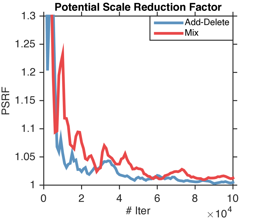
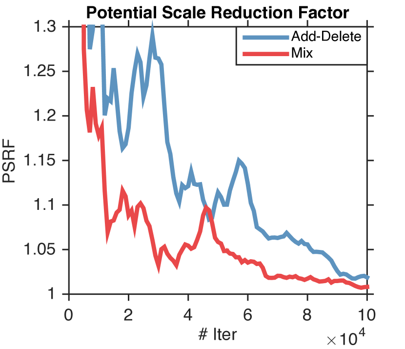
Next, we empirically study the how fast our samplers converge. We compare the strongly-Rayleigh chain in Algorithm 3 (Mix) against a simple add-delete chain (Add-Delete). To monitor the convergence of these Markov chains, we use potential scale reduction factor (PSRF) [19, 12] that runs several chains in parallel and compares within-chain variances to between-chain variances. Typically, PSRF is greater than 1 and will converge to 1 in the limit; if it is close to 1 we empirically conclude that chains have mixed. Throughout experiments we run 10 chains in parallel for estimation, and declare “convergence” at a PSRF of 1.05.

We use a Dpp on Ailerons data of size 200, and the corresponding PSRF is shown in Fig. 1(b). We observe that Mix converges slightly slower than Add-Delete since it is lazier. However, the Add-Delete chain does not always mix fast. Fig. 1(c) illustrates a different setting, where we modify the eigenspectrum of the kernel matrix: the first 100 eigenvalues are 500 and others 1/500. Such a kernel corresponds to almost an elementary Dpp, where the size of the observed subsets sharply concentrates around 100. Here, Add-Delete moves very slowly. Mix, in contrast, has the ability to exchange elements and thus converges much faster than Add-Delete.

References

- Anari and Gharan [2015] Nima Anari and Shayan O. Gharan. Effective-resistance-reducing flows and asymmetric tsp. In IEEE Symposium on Foundations of Computer Science (FOCS), 2015.
- Anari and Gharan [2014] Nima Anari and Shayan Oveis Gharan. The kadison-singer problem for strongly rayleigh measures and applications to asymmetric tsp. arXiv preprint arXiv:1412.1143, 2014.
- Anari et al. [2016] Nima Anari, Shayan Oveis Gharan, and Alireza Rezaei. Monte Carlo Markov chain algorithms for sampling strongly Rayleigh distributions and determinantal point processes. COLT, 2016.
- Bach [2013] Francis Bach. Learning with Submodular Functions: A Convex Optimization Perspective. Foundations and Trends in Machine Learning, 2013.
- Barinova et al. [2012] Olga Barinova, Victor Lempitsky, and Pushmeet Kohli. On detection of multiple object instances using Hough transforms. IEEE Trans. on Pattern Analysis and Machine Intelligence, 9:1773–1784, 2012.
- Bilmes [2013] Jeff Bilmes. Deep mathematical properties of submodularity with applications to machine learning. Tutorial at the Conference on Neural Information Processing Systems (NIPS), 2013.
- Borcea et al. [2009] Julius Borcea, Petter Brändén, and Thomas Liggett. Negative dependence and the geometry of polynomials. Journal of the American Mathematical Society, 22(2):521–567, 2009.
- Borodin [2009] Alexei Borodin. Determinantal point processes. arXiv:0911.1153, 2009.
- Borodin and Gorin [2012] Alexei Borodin and Vadim Gorin. Lectures on integrable probability, 2012.
- Borodin and Olshanski [2000] Alexei Borodin and Grigori Olshanski. Distributions on partitions, point processes, and the hypergeometric kernel. Communications in Mathematical Physics, 211(2):335–358, 2000.
- Bouchard-Côté and Jordan [2010] Alexandre Bouchard-Côté and Michael I. Jordan. Variational inference over combinatorial spaces. In NIPS, 2010.
- Brooks and Gelman [1998] Stephen P Brooks and Andrew Gelman. General methods for monitoring convergence of iterative simulations. Journal of computational and graphical statistics, pages 434–455, 1998.
- Bufetov [2012] Alexander I Bufetov. Infinite determinantal measures. arXiv:1207.6793, 2012.
- Cesa-Bianchi and Lugosi [2009] Nicolo Cesa-Bianchi and Gabor Lugosi. Combinatorial bandits. In COLT, 2009.
- Deshpande et al. [2006] Amit Deshpande, Luis Rademacher, Santosh Vempala, and Grant Wang. Matrix approximation and projective clustering via volume sampling. Theory of Computing, 2:225–247, 2006.
- Ermon et al. [2013] Stefano Ermon, Carla P Gomes, Ashish Sabharwal, and Bart Selman. Embed and project: Discrete sampling with universal hashing. In NIPS, pages 2085–2093, 2013.
- Feder and Mihail [1992] Tomás Feder and Milena Mihail. Balanced matroids. In STOC, pages 26–38, 1992.
- Frieze et al. [2014] Alan Frieze, Navin Goyal, Luis Rademacher, and Santosh Vempala. Expanders via random spanning trees. SIAM Journal on Computing, 43(2):497–513, 2014.
- Gelman and Rubin [1992] Andrew Gelman and Donald B Rubin. Inference from iterative simulation using multiple sequences. Statistical science, pages 457–472, 1992.
- Gharan et al. [2011] Shayan O. Gharan, Amin Saberi, and Mohit Singh. A randomized rounding approach to the Traveling Salesman Problem. In IEEE Symposium on Foundations of Computer Science (FOCS), 2011.
- Gotovos et al. [2015] Alkis Gotovos, Hamed Hassani, and Andreas Krause. Sampling from probabilistic submodular models. In NIPS, pages 1936–1944, 2015.
- Greig et al. [1989] Dorothy M. Greig, Bruce T. Porteous, and Allan H. Seheult. Exact maximum a posteriori estimation for binary images. Journal of the Royal Statistical Society, 51(2), 1989.
- Hough et al. [2006] J Ben Hough, Manjunath Krishnapur, Yuval Peres, and Bálint Virág. Determinantal processes and independence. Probability Surveys, 2006.
- Kang [2013] Byungkon Kang. Fast determinantal point process sampling with application to clustering. In NIPS, pages 2319–2327, 2013.
- Krause and Jegelka [2013] Andreas Krause and Stefanie Jegelka. Submodularity in Machine Learning: New directions. Tutorial at the International Conference on Machine Learning (ICML), 2013.
- Kulesza and Taskar [2012] Alex Kulesza and Ben Taskar. Determinantal point processes for machine learning. Foundations and Trends in Machine Learning. Now, 2012.
- Li et al. [2016a] Chengtao Li, Stefanie Jegelka, and Suvrit Sra. Fast DPP sampling for Nyström with application to kernel methods. ICML, 2016a.
- Li et al. [2016b] Chengtao Li, Suvrit Sra, and Stefanie Jegelka. Gaussian quadrature for matrix inverse forms with applications. ICML, 2016b.
- Lyons [2003] Russell Lyons. Determinantal probability measures. Publications Mathématiques de l’Institut des Hautes Études Scientifiques, 98:167–212, 2003.
- Lyons [2014] Russell Lyons. Determinantal probability: basic properties and conjectures. arXiv:1406.2707, 2014.
- Macchi [1975] Odile Macchi. The coincidence approach to stochastic point processes. Advances in Applied Probability, pages 83–122, 1975.
- Maddison et al. [2014] Chris J Maddison, Daniel Tarlow, and Tom Minka. A* sampling. In NIPS, 2014.
- Marcus [2016] Adam W Marcus. Polynomial convolutions and (finite) free probability, 2016.
- Mariet and Sra [2016] Zelda Mariet and Suvrit Sra. Diversity networks. In ICLR, 2016.
- Pemantle and Peres [2014] Robin Pemantle and Yuval Peres. Concentration of lipschitz functionals of determinantal and other strong rayleigh measures. Combinatorics, Probability and Computing, 23(01):140–160, 2014.
- Rebeschini and Karbasi [2015] Patrick Rebeschini and Amin Karbasi. Fast mixing for discrete point processes. COLT, 2015.
- Smith and Eisner [2008] David A. Smith and Jason Eisner. Dependency parsing by belief propagation. In EMNLP, 2008.
- Soshnikov [2000] Alexander Soshnikov. Determinantal random point fields. Russian Mathematical Surveys, 55(5):923–975, 2000.
- Spielman and Srivastava [2008] Dan Spielman and Nikhil Srivastava. Graph sparsification by effective resistances. In Symposium on Theory of Computing (STOC), 2008.
- Zhang et al. [2015] Jian Zhang, Josip Djolonga, and Andreas Krause. Higher-order inference for multi-class log-supermodular models. In ICCV, pages 1859–1867, 2015.