Probing neutrino nature at Borexino detector with chromium neutrino source

Abstract

In this paper, we indicate a possibility of utilizing the intense chromium source ($\sim 370\;PBq$) in probing the neutrino nature in low energy neutrino experiments with the ultra-low threshold and background real-time Borexino detector located near the source ($\sim 8\;m$). We analyze the elastic scattering of electron neutrinos (Dirac or Majorana, respectively) on the unpolarized electrons in the relativistic neutrino limit. We assume that the incoming neutrino beam is the superposition of left-right chiral states. Left chiral neutrinos may be detected by the standard $V-A$ and non-standard scalar $S_{L}$, tensor $T_{L}$ interactions, while right chiral ones partake only in the exotic $V+A$ and $S_{R},T_{R}$ interactions. Our model-independent study is carried out for the flavour (current) neutrino eigenstates. We compute the expected event number for the standard $V-A$ interaction of the left chiral neutrinos using the current experimental values of standard couplings and in the case of left-right chiral superposition. We show that the significant decrement in the event number due to the interference terms between the standard and exotic interactions for the Majorana $\nu_{e}$’s may appear. The $90\%\;C.L.$ sensitivity contours in the planes of corresponding exotic couplings are also found. The presence of interferences in the Majorana case give the stronger constraints than for the Dirac neutrinos, even if the neutrino source is placed outside the detector.

1 Introduction

Possibility of utilizing various artificial neutrino sources (ANS) in the low energy neutrino ($\nu$) experiments with the ultra-low background and threshold detectors to explore the Lorentz structure of weak interactions and other non-standard $\nu$ properties has been discussed in many papers, e. g. Vogel ; Ferrari ; Ianni ; Ianni1 ; Miranda . As is well known there are essentially two types of the ANS which can be used in the large liquid scintillator detectors; the monochromatic $\nu_{e}$ emitters $(e.g.^{51}Cr,^{37}Ar,^{49}V,^{145}Sm)$, and $\overline{\nu}_{e}$ sources with continuous $\beta$ spectrum (e. g. ${}^{144}Cs-^{144}Pr,^{106}Ru-^{106}Rh,^{90}Sr-^{90}Y$, ${}^{42}Ar-^{42}K$) Korn ; sterile7 . ${}^{51}Cr$ source as the dichromatic neutrino emitter with energies of $430\;keV$ $(10\;\%)$ and $750\;keV$ $(90\;\%)$, and a mean life time $(\tau\simeq 40$ days) has already been utilized to calibrate GALLEX and SAGE experiments Gallex ; Gallex1 ; Gallex2 ; Sage ; Sage1 ; Sage2 , where a deficit in the rate of $\nu$ interactions has been found Bahcall ; Giunti . Presently, the ${}^{51}Cr$ emitter with activity of the order of $\sim 370\;PBq\;(\sim 10\;MCi)$ in the SOX experiment (Short distance Oscillation with boreXino) with the Borexino detector will be used to search for the sterile $\nu_{e}$’s sterile7 ; sterile ; sterile1 ; sterile2 ; sterile3 ; sterile4 ; sterile5 ; sterile6 and to improve the current limits on the neutrino magnetic moment Beda , and to reduce the uncertainty on the direct measurement of the standard couplings. It is worthy of reminding that the extremely low background Borexino detector has precisely measured the low energy solar $\nu_{e}$ components (${}^{7}Be,pep$) Be ; Be1 ; pep and detected the geophysical $\overline{\nu}_{e}$’s geo .
This detector seems to be an appropriate tool to test the $\nu$ nature, i. e. whether $\nu$’s are the Dirac or Majorana fermions. The problem of distinguishing between the Dirac and Majorana $\nu$’s can be investigated in the context of non-vanishing $\nu$ mass and of standard vector-axial $(V-A)$ weak interaction of the only left chiral (LCh) $\nu$’s, using purely leptonic processes such as the polarized muon decay at rest or the mentioned neutrino-electron elastic scattering (NEES). Kayser Kayser and Langacker Langacker have proposed the first tests concerning the mass dependence, however it is worthwhile noting the other papers devoted to the various aspects of $\nu$ nature, e. g. Zralek ; Nishiura ; Semikoz ; Pastor ; Barranco ; Singh ; Gutierrez . It is necessary to point out that the current experiments regarding the discrimination between the Dirac and Majorana $\nu$’s are mainly based on the searching for the neutrinoless double beta decay (NDBD) Majorana , however the low energy $\nu$ experiments with the intense ANS, very low background and threshold detector seem to have similar scientific opportunities, and may also shed some light on this problem. It is important to emphasize that there is also an alternative scenario within the relativistic $\nu$ limit, when one departs from the $V-A$ interaction and one admits the exotic scalar $(S)$, tensor $(T)$, pseudoscalar $(P)$ and $(V+A)$ weak interactions of the right chiral (RCh) $\nu$’s (right-handed helicity when $m_{\nu}\rightarrow 0$) in the leptonic processes. The proper tests have been reported by Rosen Rosen and Dass Dass . It is relevant to remark that the existing data still leaves a little space for the exotic couplings of the interacting RCh $\nu$’s outside the SM SM . Let us recall that the SM does not clarify the origin of parity violation (PV) at current energies. It is well known that the SM PV is incorporated in ad hoc way by assuming that gauge boson couples only to the left chiral currents. However on the other hand, there is no experimental evidence of the parity conservation at higher energies so far. Moreover, the SM does not explain the observed baryon asymmetry of universe barion through a single CP-violating phase of the Cabibbo-Kobayashi-Maskawa quark-mixing matrix (CKM) Kobayashi , the large hierarchy fermion masses, and other fundamental aspects. Consequently, a lot of non-standard schemes with the Majorana (and Dirac) $\nu$’s, time reversal violation (TRV) exotic interactions, mechanisms explaining the origin of fermion generations, masses, mixing and smallness of $\nu$ mass appeared. It is worthwhile to mention the non-standard $\nu$ interactions (NSI) changing and conserving $\nu$ flavour NSI , which may be generated by the mechanisms of massive neutrino models massivenu . The NSI phenomenology has been extensively explored fenNSI . Concerning interacting RCh $\nu$’s, the suitable non-standard models seem to be the left-right symmetric models (LRSM) Pati , composite models (CM, where tensor and scalar interactions are generated by the exchange of constituents) Jodidio ; CM , models with extra dimensions (MED) Extra , the unparticle models (UP) unparticle . In the MED the LCh standard particles live on the three-brane, while the RCh $\nu$’s can move in the extra dimensions. It causes that the interactions of RCh $\nu$’s with the LCh fermions are extremely tiny to be observed. It is worthy of stressing that in the UP scheme the leptons with the different chiralities can couple to the spin-0 scalar, spin-1 vector, spin-2 tensor unparticle sectors. It means that the amplitude for NEES can have the form of the unparticle four-fermion contact interaction at low energies, and contain the exotic contributions. Currently there is no unambiguous indication of new non-standard gauge model, because the experimental possibilities are still limited. There is a constant necessity of improvement of the precision of present tests at low energies, and on the other hand, the precise measurements of new observables including the linear terms from the exotic couplings would be required.
In this study, we concentrate on the application of ${}^{51}Cr$ electron neutrino $(\nu_{e})$ source deployed at $8.25\;m$ from the centre of Borexino detector to find the allowed limits on the exotic $S$, $T$, $V+A$ couplings in the relativistic $\nu_{e}$ limit, when the incoming $\nu_{e}$ beam is the superposition of left-right chiral states and has Dirac or Majorana nature. We analyze the elastic scattering of $\nu_{e}$ beam off the unpolarized electron target as the detection process of possible exotic signals. It should be pointed out that the scintillator detector does not allow to observe the directionality of the recoil electrons, so all the interference terms between the standard and exotic couplings in the differential cross section vanish for the Dirac $\nu_{e}$’s, and only the contributions from the squares of exotic couplings of the RCh $\nu$’s and of non-standard couplings of LCh ones (and at most the interferences within exotic couplings) may generate the possible effect. The situation is distinct for the Majorana $\nu$’s, where some linear terms coming from the exotic couplings after the integration over the azimuthal angle of outgoing electron momentum may occur. One of the goals is to show in model-independent way how the expected event number for the standard $V-A$ interaction depends on the precision of measurement of standard couplings. Next, we calculate the predicted event number coming from the admixture of exotic interactions both for the Dirac and Majorana $\nu_{e}$’s. Finally, we find the $90\,\%\,C.L.$ sensitivity contours in the planes of proper exotic couplings for both scenarios.

2 Elastic scattering of Dirac electron neutrinos off unpolarized electrons

We assume that the incoming monochromatic Dirac $\nu_{e}$ beam comes from the electron capture by ${}^{51}Cr$ $(e^{-}+^{51}Cr\rightarrow\nu_{e}+^{51}V)$ and is the superposition of left-right chiral states. LCh $\nu_{e}$’s are mainly detected by the standard $V-A$ interaction, while RCh ones are detected only by the exotic scalar $S$, tensor $T$, $V+A$ interactions in the elastic scattering on the unpolarized electrons; $\nu_{e}+e^{-}\rightarrow\nu_{e}+e^{-}$. The considered scenario admits also the detection of $\nu_{e}$’s with left-handed chirality by the non-standard $S$ and $T$ interactions. It is important to emphasize that our analysis is carried out for the flavour (current) $\nu_{e}$ eigenstates. The amplitude for the $\nu_{e}e^{-}$ scattering at low energies takes the form:

$$M^{D}_{\nu_{e}e^{-}} = \frac{G_{F}}{\sqrt{2}}\{(\overline{u}_{e^{\prime}}\gamma^{\alpha}(c_{V}^{L}-c_{A}^{L}\gamma_{5})u_{e})(\overline{u}_{\nu_{e^{\prime}}}\gamma_{\alpha}(1-\gamma_{5})u_{\nu_{e}})$$

$$\mbox{}+(\overline{u}_{e^{\prime}}\gamma^{\alpha}(c_{V}^{R}+c_{A}^{R}\gamma_{5})u_{e})(\overline{u}_{\nu_{e^{\prime}}}\gamma_{\alpha}(1+\gamma_{5})u_{\nu_{e}})$$

$$\mbox{}+c_{S}^{R}(\overline{u}_{e^{\prime}}u_{e})(\overline{u}_{\nu_{e^{\prime}}}(1-\gamma_{5})u_{\nu_{e}})$$

$$\mbox{}+\frac{1}{2}c_{T}^{R}(\overline{u}_{e^{\prime}}\sigma^{\alpha\beta}u_{e})(\overline{u}_{\nu_{e^{\prime}}}\sigma_{\alpha\beta}(1-\gamma_{5})u_{\nu_{e}})$$

$$\mbox{}+c_{S}^{L}(\overline{u}_{e^{\prime}}u_{e})(\overline{u}_{\nu_{e^{\prime}}}(1+\gamma_{5})u_{\nu_{e}})$$

$$\mbox{}+\frac{1}{2}c_{T}^{L}(\overline{u}_{e^{\prime}}\sigma^{\alpha\beta}u_{e})(\overline{u}_{\nu_{e^{\prime}}}\sigma_{\alpha\beta}(1+\gamma_{5})u_{\nu_{e}})\},$$

where $G_{F}=1.1663788(7)\times 10^{-5}\,\mbox{GeV}^{-2}(0.6\;ppm)$ Mulan is the Fermi constant. The coupling constants are denoted with the superscripts $L$ and $R$ as $c_{V}^{L,R}$, $c_{A}^{L,R}$, $c_{S}^{R,L}$, $c_{T}^{R,L}$ respectively to the incoming $\nu_{e}$ of left- and right-handed chirality. Because we take into account the TRV, all the coupling constants are complex. It is worthy of pointing out that we probe the case when the outgoing electron direction is not observed, so the laboratory differential cross section is presented after integration over the azimuthal angle $\phi_{e}$ of the recoil electron momentum. The obtained formula, in the relativistic limit, does not contain the interference terms between the standard $c_{V,A}^{L}$ and exotic $c_{S,T}^{L,R},c_{V,A}^{R}$ couplings:

$$\frac{d\sigma}{dy_{e}}=\bigg{(}\frac{d\sigma}{dy_{e}}\bigg{)}_{(V-A)}+\bigg{(}\frac{d\sigma}{dy_{e}}\bigg{)}_{(V+A)}+\bigg{(}\frac{d\sigma}{dy_{e}}\bigg{)}_{(S,T)},$$

$$\bigg{(}\frac{d\sigma}{dy_{e}}\bigg{)}_{(V-A)}=B\bigg{\{}(1-\mbox{\boldmath$\hat{\eta}_{\nu}$}\cdot\hat{\bf q})\bigg{[}|c_{V}^{L}+c_{A}^{L}|^{2}$$

$$\mbox{}+|c_{V}^{L}-c_{A}^{L}|^{2}(1-y_{e})^{2}-\frac{m_{e}y_{e}}{E_{\nu}}\left(|c_{V}^{L}|^{2}-|c_{A}^{L}|^{2}\right)\bigg{]}\bigg{\}},$$

$$\bigg{(}\frac{d\sigma}{dy_{e}}\bigg{)}_{(V+A)}=B\bigg{\{}(1+\mbox{\boldmath$\hat{\eta}_{\nu}$}\cdot\hat{\bf q})\bigg{[}|c_{V}^{R}+c_{A}^{R}|^{2}$$

$$\mbox{}+|c_{V}^{R}-c_{A}^{R}|^{2}(1-y_{e})^{2}-\frac{m_{e}y_{e}}{E_{\nu}}\left(|c_{V}^{R}|^{2}-|c_{A}^{R}|^{2}\right)\bigg{]}\bigg{\}},$$

$$\bigg{(}\frac{d\sigma}{dy_{e}}\bigg{)}_{(S,T)}=\mbox{}B\Bigg{\{}(1+\mbox{\boldmath$\hat{\eta}_{\nu}$}\cdot\hat{\bf q})\bigg{[}\frac{1}{2}y_{e}\left(y_{e}+2\frac{m_{e}}{E_{\nu}}\right)|c_{S}^{R}|^{2}$$

$$\mbox{}+\left((2-y_{e})^{2}-\frac{m_{e}}{E_{\nu}}y_{e}\right)|{c_{T}^{R}}|^{2}+y_{e}(y_{e}-2)Re(c_{S}^{R}c_{T}^{*R})\bigg{]}$$

$$\mbox{}+(1-\mbox{\boldmath$\hat{\eta}_{\nu}$}\cdot\hat{\bf q})\bigg{[}\frac{1}{2}y_{e}\left(y_{e}+2\frac{m_{e}}{E_{\nu}}\right)|c_{S}^{L}|^{2}$$

$$\mbox{}+\left((2-y_{e})^{2}-\frac{m_{e}}{E_{\nu}}y_{e}\right)|{c_{T}^{L}}|^{2}+y_{e}(y_{e}-2)Re(c_{S}^{L}c_{T}^{*L})\bigg{]}\Bigg{\}},$$

$$y_{e} \equiv \frac{T_{e}}{E_{\nu}}=\frac{m_{e}}{E_{\nu}}\frac{2cos^{2}\theta_{e}}{(1+\frac{m_{e}}{E_{\nu}})^{2}-cos^{2}\theta_{e}}$$ (5)

is the ratio of the kinetic energy of the recoil electron $T_{e}$ to the incoming $\nu_{e}$ energy $E_{\nu}$; $\theta_{e}$ is the angle between the direction of the outgoing electron momentum $\hat{\bf p}_{e}$ and $\nu_{e}$ LAB momentum unit vector ${\bf\hat{q}}$ (recoil electron scattering angle); $m_{e}$ is the electron mass; $B\equiv\left(E_{\nu}m_{e}/2\pi\right)\left(G_{F}^{2}/2\right)$; $\hat{\eta}_{\nu}$ is the unit 3-vector of $\nu_{e}$ spin polarization in its rest frame; $(\mbox{\boldmath$\hat{\eta}_{\nu}$}\cdot\hat{\bf q}){\bf\hat{q}}$ is the longitudinal component of $\nu_{e}$ spin polarization; $|\mbox{\boldmath$\hat{\eta}_{\nu}$}\cdot\hat{\bf q}|=|1-2Q_{L}^{\nu}|$; $Q_{L}^{\nu}$ is the probability of producing the LCh $\nu_{e}$.
It can be noticed that there are only the contributions from the $T$-even longitudinal component of the $\nu_{e}$ spin polarization, and no linear terms from the exotic couplings in the relativistic limit appear. The formula on the number of events for the standard and non-standard interactions is similar as in Ianni :

$$N=N_{t}\cdot\Phi_{0}\cdot\Gamma(t_{tr},t_{ex})\cdot F(h=\frac{R}{D})\cdot\int_{250\;keV}^{700\;keV}dT_{e}^{m}\cdot$$

$$\mbox{}\bigg{[}0.81\int_{0}^{T_{e}^{max}(E_{\nu}=746\;keV)}dT_{e}R(T_{e}^{m},T_{e})\frac{d\sigma}{dT_{e}}\mid_{E_{\nu}=746\;keV}$$

$$\mbox{}+0.09\int_{0}^{T_{e}^{max}(E_{\nu}=751\;keV)}dT_{e}R(T_{e}^{m},T_{e})\frac{d\sigma}{dT_{e}}\mid_{E_{\nu}=751\;keV}\bigg{]}.$$

In order to compute the expected event number for the standard $V-A$ interaction, we use the experimental values of standard couplings: $c_{V}^{L}=1+(-0.04\pm 0.015),c_{A}^{L}=1+\\ (-0.507\pm 0.014)$ Data . Assumptions concerning the technical setup are analogical as in Ianni except the stronger source activity. $N_{e}=3.3\cdot 10^{32}$ is the number of electrons calculated for $100$ tons of spherical fiducial volume $(R=3\;m)$ of the detector; $D=8.25\;m$ is the distance between the chromium source and detector centre; $\Phi_{0}=(I_{0}/4\pi D^{2})$; $I_{0}=370\;PBq=10MCi$ is the intensity of the source at end of bombardment; $F(h=R/D)=(3/2h^{3})\{h-[(1-h^{2})/2]\;ln[(1+h)/(1-h)]\}$
$\simeq 1.028$ is the factor taking into account the geometry of the system; $\Gamma(t_{tr},t_{ex})=\tau exp(-t_{tr}/\tau)[1-exp(-t_{ex}\tau)]$;
$\tau=(T_{1/2}/ln2)\simeq 39.97$ days; $t_{tr}=5$ days; $t_{ex}=60$ days define the exposure time.

$$R(T_{e}^{m},T_{e}) = \frac{1}{\sqrt{2\pi}\delta(T_{e})}exp\left[-\frac{(T_{e}^{m}-T_{e})^{2}}{2\delta^{2}(T_{e})}\right]$$ (7)

is the detector resolution function; $\delta(T_{e})/keV=48\sqrt{T_{e}/MeV}$ is the electron energy resolution; $T_{e}^{m}\in[250,700]\;keV$ is the energy window for the reconstructed recoil electron kinetic energy.
Fig.1 shows how the uncertainty on the measurement of standard $c_{V,A}^{L}$ couplings affects the expected event number. In this case we assume pure LCh $\nu_{e}$ beam with $\mbox{\boldmath$\hat{\eta}_{\nu}$}\cdot\hat{\bf q}=-1$. Fig. 2 illustrates the dependence of event number on $\mbox{\boldmath$\hat{\eta}_{\nu}$}\cdot\hat{\bf q}\in[-1,1]$ for the standard interaction (solid thick line) and various combinations of exotic couplings (other lines). Fig. 3 demonstrates the predicted event number coming from the superposition of left-right chiral $\nu_{e}$’s for two chosen scenarios $(c_{V}^{L}$, $c_{A}^{L}$, $c_{V}^{R}$, $c_{A}^{R})$, $(c_{V}^{L}$, $c_{A}^{L}$, $c_{S}^{R}$, $c_{T}^{R})$ (upper plots) and one for the pure LCh $\nu_{e}$ beam (lower plot). We use the experimental values for the standard couplings $c_{V}^{L}=1-0.04$, $c_{A}^{L}=1-0.507$ and probe the interval $[-0.6,\;0.6]$ of all the exotic couplings. It is important to stress that for the left-right chiral superposition of $\nu_{e}$ states $\mbox{\boldmath$\hat{\eta}_{\nu}$}\cdot\hat{\bf q}\not=-1$. In order to illustrate all possible effects from the exotic interactions of RCh $\nu_{e}$’s we assume $\boldmath\hat{\eta}_{\nu}\cdot\hat{\bf q}=-0.75$ corresponding to $P_{L}=0.875$. For the scenario with only LCh $\nu_{e}$’s participating both in the standard $V-A$ and non-standard $S_{L},T_{L}$ interactions we take $\boldmath\hat{\eta}_{\nu}\cdot\hat{\bf q}=-1$. Fig. 4 illustrates $90\%\;C.L.$ sensitivity contours in the planes ($c_{V}^{R}$, $c_{A}^{R}$), ($c_{S}^{R}$, $c_{T}^{R}$), ($c_{S}^{L}$, $c_{T}^{L}$), respectively. It is worth noting that we consider six degrees of freedom and then carry out the projection onto the appropriate plane of couplings. The proper contours are calculated with the use of inequality taken from Ianni :

$$\left|\frac{N}{N_{SM}}-1\right| \geq \epsilon_{90}=3.263\frac{\delta N_{SM}}{N_{SM}},$$ (8)

where $\delta N_{SM}=\sqrt{N_{B}+N_{SM}(1+N_{SM}\delta_{A}^{2})}$ is the total $1\sigma$ uncertainty of the signal; $\delta_{A}=0.01$ is the uncertainty of source activity. We assume that the number of background events is $N_{B}=4380$ as in Ianni .

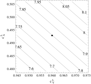
Figure 1: Dirac $\nu_{e}$. Dependence of the event number $N/10^{3}$ on the errors of the experimental values of the standard $c_{V}^{L},c_{A}^{L}$ couplings.

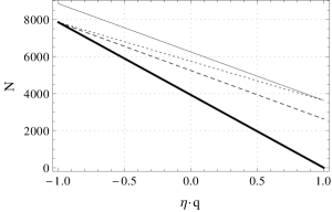
Figure 2: Dirac $\nu_{e}$. Dependence of the event number on $(\boldmath\hat{\eta}_{\nu}\cdot\hat{\bf q})\in[-1,1]$. Solid thick line for the pure standard $V-A$ interaction; dashed line, dotted line and thin line for combinations of the standard $V-A$ interaction with ($c_{V}^{R}=c_{A}^{R}=0.4,\;c_{S}^{R}=c_{T}^{R}=c_{S}^{L}=c_{T}^{L}=0$), ($c_{V}^{R}=c_{A}^{R}=c_{S}^{R}=c_{T}^{R}=0.4,\;c_{S}^{L}=c_{T}^{L}=0$) and ($c_{V}^{R}=c_{A}^{R}=c_{S}^{R}=c_{T}^{R}=c_{S}^{L}=c_{T}^{L}=0.4$) respectively.

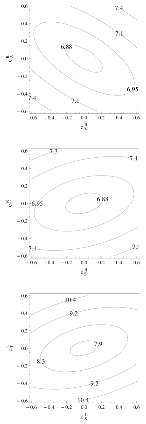
Figure 3: Dirac $\nu_{e}$. Two upper plots show the predicted event number $N/10^{3}$ coming from the superposition of left-right chiral $\nu_{e}$’s for two scenarios $(c_{V}^{L},c_{A}^{L},c_{V}^{R},c_{A}^{R})$, $(c_{V}^{L},c_{A}^{L},c_{S}^{R},c_{T}^{R})$, respectively with $\mbox{\boldmath$\hat{\eta}_{\nu}$}\cdot\hat{\bf q}=-0.75$. Lower plot concerns $(c_{V}^{L},c_{A}^{L},c_{S}^{L},c_{T}^{L})$ interactions of LCh $\nu_{e}$’s with $\mbox{\boldmath$\hat{\eta}_{\nu}$}\cdot\hat{\bf q}=-1$.

Figure 4: Dirac $\nu_{e}$. $90\%\;C.L.$ sensitivity contours in the planes ($c_{V}^{R}$, $c_{A}^{R}$), ($c_{S}^{R}$, $c_{T}^{R}$) for $\boldmath\hat{\eta}_{\nu}\cdot\hat{\bf q}=-0.75$, and the plane ($c_{S}^{L}$, $c_{T}^{L}$) with $\boldmath\hat{\eta}_{\nu}\cdot\hat{\bf q}=-1$, respectively. Dashed line of each plot is for the source located at the detector centre and for $\delta_{A}=0.001$. Dotted line is for $\delta_{A}=0.01$ and the chromium source at the detector centre. Solid line is for $D=8.25\;m$ and $\delta_{A}=0.01$.

3 Elastic scattering of Majorana electron neutrinos off unpolarized electrons

The amplitude for the elastic scattering of the Majorana $\nu_{e}$’s on the unpolarized electrons at low energies has the form (one assumes the flavour $\nu_{e}$ eigenstates similarly as for the Dirac case):

$$M^{M}_{\nu_{e}e^{-}}=\mbox{}\frac{2G_{F}}{\sqrt{2}}\{-(\overline{u}_{e^{\prime}}\gamma^{\alpha}(c_{V}-c_{A}\gamma_{5})u_{e})(\overline{u}_{\nu_{e^{\prime}}}\gamma_{\alpha}\gamma_{5}u_{\nu_{e}})$$

$$+ (\overline{u}_{e^{\prime}}\gamma^{\alpha}(\tilde{c}_{V}+\tilde{c}_{A}\gamma_{5})u_{e})(\overline{u}_{\nu_{e^{\prime}}}\gamma_{\alpha}\gamma_{5}u_{\nu_{e}})$$

$$+ c_{S}^{L}(\overline{u}_{e^{\prime}}u_{e})(\overline{u}_{\nu_{e^{\prime}}}(1-\gamma_{5})u_{\nu_{e}})+c_{S}^{R}(\overline{u}_{e^{\prime}}u_{e})(\overline{u}_{\nu_{e^{\prime}}}(1+\gamma_{5})u_{\nu_{e}})\}.$$

One can see that the neutrino part of the above amplitude does not contain the contribution from the $V$ and $T$ interactions in contrast to the Dirac case, where both terms partake. The $V+A$ interaction is also admitted. Moreover, the $A$ and $S$ contributions are multiplied by factor 2 and this is a direct consequence of the fact that the Majorana neutrino is described by the self-conjugate field. The indexes $L$, ($R$) for $c_{V},c_{A}\;(\tilde{c}_{V},\tilde{c}_{A})$ couplings are omitted. It means that both LCh and RCh $\nu_{e}$’s may participate in the standard A and non-standard $\tilde{A}$ interactions of Majorana $\nu_{e}$’s off the electron target. The exotic $S$ coupling constants are denoted with the superscripts $L$ and $R$ as $c_{S}^{L,R}$ respectively to the incoming $\nu_{e}$ of left- and right-handed chirality. All the couplings are assumed to be complex numbers as for the Dirac case. The differential cross section for the elastic scattering of Majorana current $\nu_{e}$’s on the unpolarized electrons in the relativistic limit has the form:

$$\frac{d\sigma}{dy_{e}}=\bigg{(}\frac{d\sigma}{dy_{e}}\bigg{)}_{(V-A)} + \bigg{(}\frac{d\sigma}{dy_{e}}\bigg{)}_{(\tilde{V}+\tilde{A})}$$ (10)

$$\mbox{}+\bigg{(}\frac{d\sigma}{dy_{e}}\bigg{)}_{(V-A)(\tilde{V}+\tilde{A})} + \bigg{(}\frac{d\sigma}{dy_{e}}\bigg{)}_{(S_{L},S_{R})},$$

$$\bigg{(}\frac{d\sigma}{dy_{e}}\bigg{)}_{(V-A)}=\mbox{}B\bigg{\{}-\frac{2m_{e}y_{e}}{E_{\nu}}\left(|c_{V}|^{2}-|c_{A}|^{2}\right)$$

$$\mbox{}+|c_{V}+c_{A}|^{2}(2+(1+\mbox{\boldmath$\hat{\eta}_{\nu}$}\cdot\hat{\bf q})(y_{e}-2)y_{e})$$

$$\mbox{}+|c_{V}-c_{A}|^{2}(2+(1-\mbox{\boldmath$\hat{\eta}_{\nu}$}\cdot\hat{\bf q})(y_{e}-2)y_{e})\bigg{\}},$$

$$\bigg{(}\frac{d\sigma}{dy_{e}}\bigg{)}_{(\tilde{V}+\tilde{A})}=\mbox{}B\bigg{\{}-\frac{2m_{e}y_{e}}{E_{\nu}}\left(|\tilde{c}_{V}|^{2}-|\tilde{c}_{A}|^{2}\right)$$ (12)

$$\mbox{}+|\tilde{c}_{V}-\tilde{c}_{A}|^{2}(2+(1+\mbox{\boldmath$\hat{\eta}_{\nu}$}\cdot\hat{\bf q})(y_{e}-2)y_{e})$$

$$\mbox{}+|\tilde{c}_{V}+\tilde{c}_{A}|^{2}(2+(1-\mbox{\boldmath$\hat{\eta}_{\nu}$}\cdot\hat{\bf q})(y_{e}-2)y_{e})\bigg{\}},$$

$$\bigg{(}\frac{d\sigma}{dy_{e}}\bigg{)}_{(V-A)(\tilde{V}+\tilde{A})}$$

$$= \mbox{}4B\bigg{\{}Re(c_{A}\tilde{c}_{A}^{*})\bigg{(}2+(y_{e}-2)y_{e}+\frac{m_{e}y_{e}}{E_{\nu}}\bigg{)}$$

$$\mbox{}+\bigg{(}Re(c_{V}\tilde{c}_{A}^{*})-Re(c_{A}\tilde{c}_{V}^{*})\bigg{)}(y_{e}-2)y_{e}\mbox{\boldmath$\hat{\eta}_{\nu}$}\cdot\hat{\bf q}$$

$$\mbox{}+Re(c_{V}\tilde{c}_{V}^{*})\bigg{(}-2-(y_{e}-2)y_{e}+\frac{m_{e}y_{e}}{E_{\nu}}\bigg{)}\bigg{\}},$$

$$\bigg{(}\frac{d\sigma}{dy_{e}}\bigg{)}_{(S_{L},S_{R})}=\mbox{}B\bigg{\{}2y_{e}\left(y_{e}+2\frac{m_{e}}{E_{\nu}}\right)$$

$$\mbox{}\cdot\bigg{[}(1+\mbox{\boldmath$\hat{\eta}_{\nu}$}\cdot\hat{\bf q})|c_{S}^{R}|^{2}+(1-\mbox{\boldmath$\hat{\eta}_{\nu}$}\cdot\hat{\bf q})|c_{S}^{L}|^{2}\bigg{]}\bigg{\}}.$$

We see that the interference terms between ($c_{V}$, $c_{A}$) and ($\tilde{c}_{V}$, $\tilde{c}_{A}$) couplings appear in contrast to the Dirac case, where such contributions annihilate. It can also be noticed that the differential cross section does not contain $T$-odd observables similarly as for the Dirac $\nu_{e}$’s. It is obvious that the predicted event number for the pure $V-A$ interaction in the Majorana case is the same as for the Dirac $\nu_{e}$’s. However if one departs from the standard couplings and allows for the exotic interactions, the possibility of distinguishing between the Dirac and Majorana $\nu$’s in the limit o vanishing $\nu_{e}$ mass due to the interferences appears. Fig. 5 shows how the event number depends on $\boldmath\hat{\eta}_{\nu}\cdot\hat{\bf q}\in[-1,1]$ in the standard case and for the exotic interactions. It is noteworthy that the presence of interference terms may cause a decrease of event number (thin line) in contrast to the Dirac scenario, where such a regularity is impossible. Fig. 6 illustrates the predicted event number for the superposition of left-right chiral $\nu_{e}$’s in the case of two scenarios. Upper plot shows clearly the impact of the interferences between ($c_{V}$, $c_{A}$) and ($\tilde{c}_{V}$, $\tilde{c}_{A}$) on the event number for given $\boldmath\hat{\eta}_{\nu}\cdot\hat{\bf q}=-0.75$. The significant decrement in the event number in comparison with the Dirac case It can be noticed. Fig. 7 demonstrates $90\%\;C.L.$ sensitivity contours in the planes ($\tilde{c}_{V}$, $\tilde{c}_{A}$), ($c_{S}^{L}$, $c_{S}^{R}$), respectively. In the present case we admit forth degrees of freedom for the Majorana $\nu_{e}$’s (inequality (8) with $\epsilon_{90}=2.789(\delta N_{SM}/N_{SM})$ and then carry out the projection onto the appropriate plane of couplings. One can see the qualitative difference due to the interferences in comparison with the Dirac case, even when the source is placed at $D=8.25\;m$ with $\delta_{A}=0.01$ (solid line).

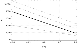
Figure 5: Majorana $\nu_{e}$.Dependence of the event number on $(\boldmath\hat{\eta}_{\nu}\cdot\hat{\bf q})\in[-1,1]$. Solid thick line for the pure standard $V-A$ interaction; dashed line, dotted line and thin line for combinations of the standard $V-A$ interaction with ($\tilde{c}_{V}=\tilde{c}_{A}=0.4,\;c_{S}^{L}=c_{S}^{R}=0$), ($\tilde{c}_{V}=\tilde{c}_{A}=c_{S}^{L}=c_{S}^{R}=0.4$) and ($\tilde{c}_{V}=0.2,\;\tilde{c}_{A}=-0.2,\;c_{S}^{L}=c_{S}^{R}=0.4$) respectively.

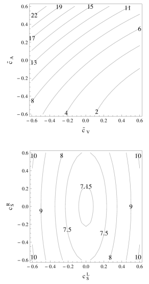
Figure 6: Majorana $\nu_{e}$. Upper plot shows the expected event number $N/10^{3}$ for nonzero ($c_{V}$, $c_{A}$, $\tilde{c}_{V}$, $\tilde{c}_{A}$) couplings; the interferences between ($c_{V}$, $c_{A}$) and ($\tilde{c}_{V}$, $\tilde{c}_{A}$) can significantly decrease the event number. Lower plot is for nonzero ($c_{V}$, $c_{A}$, $c_{S}^{L}$, $c_{S}^{R}$). Both cases with $\boldmath\hat{\eta}_{\nu}\cdot\hat{\bf q}=-0.75$.

Figure 7: Majorana $\nu_{e}$. $90\%\;C.L.$ sensitivity contours in the planes ($\tilde{c}_{V}$, $\tilde{c}_{A}$), ($c_{S}^{L}$, $c_{S}^{R}$) for $\boldmath\hat{\eta}_{\nu}\cdot\hat{\bf q}=-0.75$. Dashed line of each plot is for the source located at the detector centre and $\delta_{A}=0.001$. Dotted line is for $\delta_{A}=0.01$ and the chromium source at the detector centre. Solid line for $D=8.25\;m$ and $\delta_{A}=0.01$.

4 Conclusions

We have shown that the high-precision low-energy experiment with the intense ${}^{51}Cr$ $\nu_{e}$ source located at near distance from the ultra-low threshold Borexino detector centre may be useful tool to test the $\nu$ nature problem in the limit of relativistic $\nu$. It is important to stress that the interference terms between $c_{V,A}$ and $\tilde{c}_{V,A}$ couplings for the Majorana $\nu_{e}$’s do not vanish. It means that even if the intense ${}^{51}Cr$ source is deployed outside the Borexino detector, the significant decrement in the event number caused by the mentioned interferences may occur. Such a regularity in the Dirac case does not manifest (no linear contributions from the exotic couplings survive). Although the chromium source can not be placed at the detector centre, such a location would allow more sensitive tests of the exotic couplings and of the $\nu$ nature, provided that the errors on the activity source are very tiny. As is known the beta emitter $(^{144}Cs-^{144}Pr)$ with the deployment at the detector centre is considered, so the combined analysis for both sources would constrain stringently the allowed region on the exotic couplings and shed more light on the fundamental question of $\nu$ nature (in preparation).

References

- (1) P. Vogel, J. Engel, Phys. Rev. D 39, 3378 (1989)
- (2) N. Ferrari, G. Fiorentini, B. Ricci, Phys. Lett. B 387, 427 (1996)
- (3) A. Ianni, D. Montanino, G. Scioscia, Eur. Phys. J. C 8, 609 (1999)
- (4) A. Ianni, D. Montanino, Astrop. Phys. 10, 331 (1999)
- (5) O. G. Miranda, V. B. Semikoz, J. W. F. Valle, Phys. Rev. D 58, 013007 (1998)
- (6) V. Kornoukhov, ITEP report No. 90, Moscow, 1994
- (7) M. Cribier et al., Phys. Rev. Lett. 107, 201801 (2011)
- (8) P. Anselmann et al., Phys. Lett. B 342, 440 (1995)
- (9) M. Cribier et al., Nucl. Instrum. Methods Phys. Res., Sect. A 378, 233 (1996)
- (10) W. Hampel et al., Phys. Lett. B 420, 114 (1998)
- (11) J. N. Abdurashitov et. al., Phys. Rev. Lett. 23 4708 (1996)
- (12) J. N. Abdurashitov et al., Phys. Rev. C 59, 2246 (1999)
- (13) J.N. Abdurashitov et al., Phys. Rev. C 73, 045805 (2006)
- (14) J. Bahcall, P. Krastev, E. Lisi, Phys. Lett. B 348, 121 (1995)
- (15) C. Giunti, M. Laveder, Phys. Rev. C 83, 065504 (2011)
- (16) C. Athanassopoulos et al., Phys. Rev. Lett. 75, 2650 (1995)
- (17) C. Athanassopoulos et al., Phys. Rev. C 54, 2685 (1996)
- (18) A. Aguilar et al., Phys. Rev. D 64, 112007 (2001)
- (19) A. Anguilar-Arevalo et al., Phys. Rev. Lett. 105, 181801 (2010)
- (20) Th. Mueller et al., Phys. Rev. C 83, 054615 (2011)
- (21) P. Huber, Phys. Rev. C 84, 024617 (2011)
- (22) G. Mention et al., Phys. Rev. D 83, 073006 (2011)
- (23) A. G. Beda et al., Phys. Part. Nucl. Lett. 10, 139 (2013)
- (24) G. Bellini et al., Phys. Rev. Lett. 107, 141302 (2011)
- (25) G. Bellini et al., Phys. Lett. B 707, 22 (2012)
- (26) G. Bellini et al., Phys. Rev. Lett. 108, 051302 (2012)
- (27) G. Bellini et al., Phys. Lett. B 687, 299 (2010)
- (28) B. Kayser, R. E. Shrock, Phys. Lett. B 112, 137 (1982)
- (29) P. Langacker, D. London, Phys. Rev. D 39, 266 (1989)
- (30) M. Zrałek, Acta Phys. Polon. B 28, 2225 (1997)
- (31) M. Doi, T. Kotani, H. Nishiura, K. Okuda and E. Takasugi, Prog. Theor. Phys. 67, 281 (1982)
- (32) V. B. Semikoz, Nucl. Phys. B 498, 39 (1997)
- (33) S. Pastor, J. Segura, V. B. Semikoz, J. W. F. Valle, Phys. Rev. D 59, 013004 (1998)
- (34) J. Barranco et al., Phys. Lett. B 739, 343 (2014)
- (35) D. Singh, N. Mobed, G. Papini, Phys. Rev. Lett. 97, 041101 (2006)
- (36) T. D. Gutierrez, Phys. Rev. Lett. 96, 121802 (2006)
- (37) M. Doi et al., Phys. Lett. B 103, 219 (1981); W. C. Haxton et al., Phys. Rev. Lett. 47, 153 (1981); H. Ejiri, J. Phys. Soc. Jpn. 74, 2101 (2005)
- (38) S. P. Rosen, Phys. Rev. Lett. 48, 842 (1982)
- (39) G. V. Dass, Phys. Rev. D 32, 1239 (1985)
- (40) S. L. Glashow, Nucl. Phys. 22, 579 (1961); S. Weinberg, Phys. Rev. Lett. 19, 1264 (1967); A. Salam, A. Salam, in Elementary Particle Theory (Almquist and Wiksells, Stockholm, 1969); R. P. Feynman, M. Gell-Mann, Phys. Rev. 109, 193 (1958); E. C. G. Sudarshan, R. E. Marshak, Phys. Rev. 109, 1860 (1958)
- (41) A. Riotto, M. Trodden, Annu. Rev. Nucl. Part. Sci. 49, 35 (1999)
- (42) M. Kobayashi, T. Maskawa, Prog. Theor. Phys. 49, 652 (1973)
- (43) L. Wolfenstein, Phys. Rev. D 17, 2369 (1978); J.W.F. Valle, Phys. Lett. B 199, 432 (1987); E. Roulet, Phys. Rev. D 44, 935 (1991); M.M. Guzzo, A. Masiero, S.T. Petcov, Phys. Lett. B 260, 154 (1991).
- (44) J. Schechter, J. W. F. Valle, Phys. Rev. D 22, 2227 (1980); A. Zee, Phys. Lett. B 93, 389 (1980); L. J. Hall, V. A. Kostelecky, S. Raby, Nuclear Physics B 267, 415 (1986); K. S. Babu, Phys. Lett. B 203, 132 (1988); M. Hirsch, J. W. F. Valle, New J. Phys. 6, 76 (2004)
- (45) N. Fornengo et al., Phys. Rev. D 65, 013010 (2001); P. S. Amanik, G. M. Fuller, B. Grinstein, Astropart. Phys. 24, 160 (2005); G. L. Fogli, E. Lisi, A. Mirizzi D. Montanino, Phys. Rev. D 66, 013009 (2002); A. Esteban-Pretel, R. Tomas, J. W. F. Valle, Phys. Rev. D 76, 053001 (2007); O. G. Miranda, M. Maya, R. Huerta, Phys. Rev. D 53, 1719 (1996); O. G. Miranda, V. Semikoz, J. W. F. Valle, Nucl. Phys. Proc. Suppl. 66, 261 (1998); J. Barranco, O. G. Miranda, T. I. Rashba, Phys. Rev. D 76, 073008 (2007); A. Bolanos et al., Phys. Rev. D 79, 113012 (2009); S. Davidson et al., JHEP 0303, 011 (2003); J. Barranco et al., Phys. Rev. D 73, 113001 (2006); J. Barranco et al., Phys. Rev. D 77, 093014 (2008); C. Biggio, M. Blennow, E. Fernandez-Martinez, JHEP 0903, 139 (2009); C. Biggio, M. Blennow, E. Fernandez-Martinez, JHEP 0908, 090 (2009); J. Barranco, O. G. Miranda, T. I. Rashba, JHEP 0512, 021 (2005); K. Scholberg, Phys. Rev. D 73, 033005 (2006)
- (46) J.C. Pati, A. Salam, Phys. Rev. D 10, 275 (1974); R. Mohapatra, J.C. Pati, Phys. Rev. D 11, 566 (1975); Phys. Rev. D 11, 558 (1975); R.N. Mohapatra, G. Senjanovic, Phys. Rev. D 12, 1502 (1975); Phys Rev D 23, 165 (1981); M. A. B. Beg et al., Phys. Rev. Lett. 38, 1252 (1977); P. Herczeg, Phys. Rev. D 34, 3449 (1986)
- (47) A. Jodidio et al., Phys. Rev. D 34, 1967 (1986)
- (48) E. J. Eichten, K. D. Lane, M.E. Peskin, Phys. Rev. Lett. 50, 811 (1983); P. Herczeg, Prog. Part. Nucl. Phys. 46, 413 (2001)
- (49) N. Arkani-Hamed, S. Dimopoulous, G. Dvali, J. March-Russell, Phys. Lett. B 429, 263 (1998).
- (50) T. Banks, A. Zaks, Nucl. Phys. B 196, 189 (1982); H. Georgi, Phys. Rev. Lett. 98, 221601 (2007); H. Georgi, Phys. Lett. B 650, 275 (2007); K. Cheung, W.Y. Keung, T.C. Yuan, Phys. Rev. Lett 99, 051803 (2007); K. Cheung, W.Y. Keung, T.C. Yuan, Phys. Rev. D 76, 055003 (2007); S. L. Chen, X. G. He, Phys. Rev. D 76, 091702 (2007); A. B. Balantekin, K. O. Ozansoy, Phys. Rev. D 76, 095014 (2007); J. Barranco et al., Phys. Rev. D 79, 073011 (2009); D. Montanino, M. Picariello, J. Pulido, Phys. Rev. D 77, 093011 (2008); S. Zhou, Phys. Lett. B 659, 336 (2008); B. Grinstein, K. A. Intriligator, I. Z. Rothstein, Phys. Lett. B 662, 367 (2008); M. Deniz et al., Phys. Rev. D 82, 033004 (2010); J. Barranco et al., Int. J. Mod. Phys. A 27, 1250147 (2012)
- (51) D. M. Webber et al., Phys. Rev. Lett. 106, 041803 (2011)
- (52) K.A. Olive et al. (Particle Data Group), Chin. Phys. C 38, 090001 (2014)