Continuous tenor extension
of affine LIBOR models with multiple curves
and applications to XVA

Antonis Papapantoleon  and  Robert Wardenga Institute of Mathematics, University of Mannheim, 68131 Mannheim, Germany papapan@math.uni-mannheim.de Institut für Mathematische Stochastik, TU Dresden, 01062 Dresden, Germany Robert.Wardenga@tu-dresden.de
Abstract.

We consider the class of affine LIBOR models with multiple curves, which is an analytically tractable class of discrete tenor models that easily accommodates positive or negative interest rates and positive spreads. By introducing an interpolating function, we extend the affine LIBOR models to a continuous tenor and derive expressions for the instantaneous forward rate and the short rate. We show that the continuous tenor model is arbitrage-free, that the analytical tractability is retained under the spot martingale measure, and that under mild conditions an interpolating function can be found such that the extended model fits any initial forward curve. This allows us to compute value adjustments (i.e. XVAs) consistently, by solving the corresponding ‘pre-default’ BSDE. As an application, we compute the price and value adjustments for a basis swap, and study the model risk associated to different interpolating functions.

Key words and phrases:
Affine LIBOR models, multiple curves, discrete tenor, continuous tenor, interpolation, XVA, model risk.
2010 Mathematics Subject Classification:
91G30, 91G20, 60G44
RW acknowledges funding from the Excellence Initiative of the German Research Foundation (DFG) under grant ZUK 64. Financial support from the Europlace Institute of Finance project “Post-crisis models for interest rate markets” is gratefully acknowledged.

1. Introduction

In the aftermath of the credit crisis and the European sovereign debt crisis, several of the classical paradigms in finance were no longer able to describe the new reality and needed to be designed afresh. On the one hand, significant spreads have appeared between rates of different tenors, which led to the development of multiple curve interest rate models. On the other hand, counterparty credit risk has emerged as the native form of default risk, along with liquidity risk, funding constraints and the collateralization of trades. Therefore, in post-crisis markets the quoted price of a derivative product (or, better, the cost of its hedging portfolio) is computed as the ‘clean’ price of the product together with several value adjustments that reflect counterparty credit risk, liquidity risk, funding constraints, etc. In the context of interest rate derivatives, the ‘clean’ price is typically computed as the discounted expected payoff under a martingale measure using a (discrete tenor) LIBOR market model, while the value adjustments are provided via the solution of a BSDE, which requires the existence of a short rate to discount the cash flows.

The aim of this work is to compute prices and value adjustments consistently, in the sense that we only calibrate a discrete tenor LIBOR model and then infer the dynamics of the short rate from it, instead of resorting to an additional, external short rate model. In the sequel we will work with the class of affine LIBOR models with multiple curves. This class of models easily produces positive interest rates and positive spreads, as well as negative interest rates alongside positive spreads. Moreover, the models are analytically tractable in the sense that the driving process remains affine under all forward measures, which allows to derive explicit expressions for the prices of caplets and semi-analytic expressions for swaptions. Thus these models can be efficiently calibrated to market data; cf. Grbac et al. (2015) for more details.

Once the affine LIBOR model has been set up, we introduce an interpolating function that allows to extend the model from a discrete to a continuous tenor, and derive explicit expressions for the dynamics of the instantaneous forward rate and of the short rate. This part follows and extends Keller-Ressel (2009), while a similar interpolation for affine LIBOR models has been recently introduced by Cuchiero et al. (2016). Moreover, we show that the resulting continuous tenor model is arbitrage-free and belongs to the class of affine term structure models. Let us mention that, on the contrary, the arbitrage-free interpolation of ‘classical’ LIBOR market models is a challenging task; see e.g. Beveridge and Joshi (2012). In addition, we show that the driving process remains an affine process under the spot martingale measure, hence also the short rate is analytically tractable under this measure. The choice of the interpolating function is not innocuous though, as it may lead to undesirable behavior of the short rate; e.g. it may induce jumps at fixed times. Thus we investigate what properties the (discrete tenor) affine LIBOR model and the interpolating function should have in order to avoid such situations. In particular, we show that under mild assumptions there exists an interpolating function such that the extended model can fit any initial forward curve.

Then, we can compute value adjustments via solutions of a ‘pre-default’ BSDE using the framework of Crépey (2015a, b). As an illustration, we design and calibrate an affine LIBOR model, and consider a simple post-crisis interest rate derivative, namely a basis swap. Using the methodology outlined above, we derive the dynamics of the short rate and of the basis swap using an interpolating function, and compute the value adjustments for different specifications of the contract. As the choice of an interpolating function is still arbitrary, we study the model risk associated to different choices.

This paper is organized as follows: Section 2 reviews affine processes and Section 3 presents an overview of multiple curve markets and affine LIBOR models. Section 4 focuses on the continuous tenor extension of affine LIBOR models and studies the properties of interpolating functions. The final Section 5 outlines the computation of value adjustments in affine LIBOR models, and discusses the model risk associated with the choice of interpolating functions. The appendix contains a useful result on the time integration of affine processes.

2. Affine processes on 0dsuperscriptsubscriptabsent0𝑑\mathbb{R}_{\geqslant 0}^{d}

This section provides a brief overview of the basic notions and properties of affine processes. Proofs and further details can be found in Duffie et al. (2003), in Keller-Ressel (2008), and in Filipović (2005) for the time-inhomogeneous case.

Let (Ω,,𝔽,)Ω𝔽(\Omega,\mathcal{F},\mathbb{F},\mathds{P}) denote a complete stochastic basis in the sense of Jacod and Shiryaev (2003, Def. I.1.3), where 𝔽=(t)t[0,T]𝔽subscriptsubscript𝑡𝑡0𝑇\mathbb{F}=(\mathcal{F}_{t})_{t\in[0,T]} and T[0,)𝑇0T\in[0,\infty) denotes the time horizon. In the sequel, we will consider a process X𝑋X that satisfies the following:

Assumption (𝔸𝔸\mathbb{A}).

Let (X,(x)xD)𝑋subscriptsubscriptxx𝐷(X,(\mathds{P}_{\mathrm{x}})_{\mathrm{x}\in D}) be a conservative, time-homogeneous, stochastically continuous Markov process taking values in D=0d𝐷superscriptsubscriptabsent0𝑑D=\mathbb{R}_{\geqslant 0}^{d}, i.e. (x)xDsubscriptsubscriptxx𝐷(\mathds{P}_{\mathrm{x}})_{\mathrm{x}\in D} is a family of probability measures on (Ω,)Ω(\Omega,\mathcal{F}) and X=(Xt)t[0,T]𝑋subscriptsubscript𝑋𝑡𝑡0𝑇X=(X_{t})_{t\in[0,T]} is a Markov process such that for every xDx𝐷\mathrm{x}\in D it holds X0=xsubscript𝑋0xX_{0}=\mathrm{x}, xsubscriptx\mathds{P}_{\mathrm{x}}-almost surely. Denote by 𝔼xsubscript𝔼x\mathds{E}_{\mathrm{x}} the expectation w.r.t. the measure xsubscriptx\mathds{P}_{\mathrm{x}} and by ,\langle\cdot,\cdot\rangle the inner product in dsuperscript𝑑\mathbb{R}^{d}. Setting

T={ud:𝔼x[eu,XT]<,for all xD},subscript𝑇conditional-set𝑢superscript𝑑formulae-sequencesubscript𝔼xdelimited-[]superscripte𝑢subscript𝑋𝑇for all x𝐷\mathcal{I}_{T}=\left\{u\in\mathbb{R}^{d}\colon\mathds{E}_{\mathrm{x}}\big{[}\mathrm{e}^{\left\langle u,X_{T}\right\rangle}\big{]}<\infty,\;\mbox{for all }\mathrm{x}\in D\right\},

we assume that

  1. (i)

    0T0superscriptsubscript𝑇0\in\mathcal{I}_{T}^{\circ}, where Tsuperscriptsubscript𝑇\mathcal{I}_{T}^{\circ} denotes the interior of Tsubscript𝑇\mathcal{I}_{T};

  2. (ii)

    the conditional moment generating function of Xtsubscript𝑋𝑡X_{t} under xsubscriptx\mathds{P}_{\mathrm{x}} has exponentially-affine dependence on xx\mathrm{x}; that is, there exist functions ϕ:[0,T]×T:italic-ϕ0𝑇subscript𝑇\phi\colon[0,T]\times\mathcal{I}_{T}\rightarrow\mathbb{R} and ψ:[0,T]×Td:𝜓0𝑇subscript𝑇superscript𝑑\psi\colon[0,T]\times\mathcal{I}_{T}\rightarrow\mathbb{R}^{d} such that

    𝔼x[expu,Xt]=exp(ϕt(u)+ψt(u),x),subscript𝔼xdelimited-[]𝑢subscript𝑋𝑡subscriptitalic-ϕ𝑡𝑢subscript𝜓𝑡𝑢x\mathds{E}_{\mathrm{x}}\big{[}\exp\langle u,X_{t}\rangle\big{]}=\exp\big{(}\phi_{t}(u)+\left\langle\psi_{t}(u),\mathrm{x}\right\rangle\big{)}, (2.1)

    for all (t,u,x)[0,T]×T×D𝑡𝑢𝑥0𝑇subscript𝑇𝐷(t,u,x)\in[0,T]\times\mathcal{I}_{T}\times D.

The functions ϕitalic-ϕ\phi and ψ𝜓\psi satisfy the semi-flow equations, that is, for all 0t+sT0𝑡𝑠𝑇0\leq t+s\leq T and uT𝑢subscript𝑇u\in\mathcal{I}_{T}

ϕt+s(u)=ϕt(u)+ϕs(ψt(u)),ψt+s(u)=ψs(ψt(u)),formulae-sequencesubscriptitalic-ϕ𝑡𝑠𝑢subscriptitalic-ϕ𝑡𝑢subscriptitalic-ϕ𝑠subscript𝜓𝑡𝑢subscript𝜓𝑡𝑠𝑢subscript𝜓𝑠subscript𝜓𝑡𝑢\displaystyle\begin{split}\phi_{t+s}(u)&=\phi_{t}(u)+\phi_{s}(\psi_{t}(u)),\\ \psi_{t+s}(u)&=\psi_{s}(\psi_{t}(u)),\end{split} (2.2)

with initial conditions

ϕ0(u)=0 and ψ0(u)=u.formulae-sequencesubscriptitalic-ϕ0𝑢0 and subscript𝜓0𝑢𝑢\phi_{0}(u)=0\quad\mbox{ and }\quad\psi_{0}(u)=u.

Using the semi-flow equations we can derive the generalized Riccati equations

tϕt(u)=F(ψt(u)),ϕ0(u)=0,tψt(u)=R(ψt(u)),ψ0(u)=u,\displaystyle\begin{split}\frac{\partial}{\partial t}\phi_{t}(u)&=F(\psi_{t}(u)),\qquad\phi_{0}(u)=0,\\ \frac{\partial}{\partial t}\psi_{t}(u)&=R(\psi_{t}(u)),\qquad\psi_{0}(u)=u,\end{split} (2.3)

for (t,u)[0,T]×T𝑡𝑢0𝑇subscript𝑇(t,u)\in[0,T]\times\mathcal{I}_{T}, where F𝐹F and R=(R1,,Rd)𝑅subscript𝑅1subscript𝑅𝑑R=(R_{1},\dots,R_{d}) are functions of Lévy–Khintchine form:

F(u)=b,u+D(eξ,u1)m(dξ),Ri(u)=βi,u+αi2u,u+D(eξ,u1u,hi(ξ))μi(dξ),\displaystyle\begin{split}F(u)&=\langle b,u\rangle+\int_{D}\big{(}\mathrm{e}^{\langle\xi,u\rangle}-1\rangle\big{)}m(\mathrm{d}\xi),\\ R_{i}(u)&=\langle\beta_{i},u\rangle+\Big{\langle}\frac{\alpha_{i}}{2}u,u\Big{\rangle}+\int_{D}\big{(}\mathrm{e}^{\langle\xi,u\rangle}-1-\langle u,h_{i}(\xi)\rangle\big{)}\mu_{i}(\mathrm{d}\xi),\end{split} (2.4)

while (b,m,αi,βi,μi)1idsubscript𝑏𝑚subscript𝛼𝑖subscript𝛽𝑖subscript𝜇𝑖1𝑖𝑑(b,m,\alpha_{i},\beta_{i},\mu_{i})_{1\leq i\leq d} are admissible parameters—see Definition 2.6 in Duffie et al. (2003) for details—and hi:0dd:subscript𝑖superscriptsubscriptabsent0𝑑superscript𝑑h_{i}\colon\mathbb{R}_{\geqslant 0}^{d}\rightarrow\mathbb{R}^{d} are suitable truncation functions. The infinitesimal generator of a process satisfying Assumption (𝔸𝔸\mathbb{A}) is provided by

𝒜f(x)𝒜𝑓𝑥\displaystyle\mathcal{A}f(x) =b+i=1dβixi,f(x)+12i=1dαi,klxi2xkxlf(x)absent𝑏superscriptsubscript𝑖1𝑑subscript𝛽𝑖subscript𝑥𝑖𝑓𝑥12superscriptsubscript𝑖1𝑑subscript𝛼𝑖𝑘𝑙subscript𝑥𝑖superscript2subscript𝑥𝑘subscript𝑥𝑙𝑓𝑥\displaystyle=\left\langle b+\sum_{i=1}^{d}\beta_{i}x_{i},\nabla f(x)\right\rangle+\frac{1}{2}\sum_{i=1}^{d}\alpha_{i,kl}x_{i}\frac{\partial^{2}}{\partial x_{k}\partial x_{l}}f(x)
+D(f(x+ξ)f(x))m(dξ)subscript𝐷𝑓𝑥𝜉𝑓𝑥𝑚d𝜉\displaystyle\quad+\int_{D}\big{(}f(x+\xi)-f(x)\big{)}m(\mathrm{d}\xi) (2.5)
+i=1dD(f(x+ξ)f(x)hi(ξ),f(x))xiμi(dξ),superscriptsubscript𝑖1𝑑subscript𝐷𝑓𝑥𝜉𝑓𝑥subscript𝑖𝜉𝑓𝑥subscript𝑥𝑖subscript𝜇𝑖d𝜉\displaystyle\quad+\sum_{i=1}^{d}\int_{D}\big{(}f(x+\xi)-f(x)-\langle h_{i}(\xi),\nabla f(x)\rangle\big{)}x_{i}\mu_{i}(\mathrm{d}\xi),

for all fC02(D)𝑓superscriptsubscript𝐶02𝐷f\in C_{0}^{2}(D) and xD𝑥𝐷x\in D.

Additional results are summarized in the following lemma. In the sequel, inequalities have to be understood componentwise, in the sense that (a1,a2)(b1,b2)subscript𝑎1subscript𝑎2subscript𝑏1subscript𝑏2(a_{1},a_{2})\leq(b_{1},b_{2}) if and only if a1b1subscript𝑎1subscript𝑏1a_{1}\leq b_{1} and a2b2subscript𝑎2subscript𝑏2a_{2}\leq b_{2}.

Lemma 2.1.

The functions ϕitalic-ϕ\phi and ψ𝜓\psi satisfy the following:

  1. (1)

    ϕt(0)=ψt(0)=0subscriptitalic-ϕ𝑡0subscript𝜓𝑡00\phi_{t}(0)=\psi_{t}(0)=0 for all t[0,T]𝑡0𝑇t\in[0,T].

  2. (2)

    Tsubscript𝑇\mathcal{I}_{T} is a convex set; moreover for each t[0,T]𝑡0𝑇t\in[0,T], the functions uϕt(u)maps-to𝑢subscriptitalic-ϕ𝑡𝑢u\mapsto\phi_{t}(u) and uψt(u)maps-to𝑢subscript𝜓𝑡𝑢u\mapsto\psi_{t}(u), for uT𝑢subscript𝑇u\in\mathcal{I}_{T}, are (componentwise) convex.

  3. (3)

    ϕt()subscriptitalic-ϕ𝑡\phi_{t}(\cdot) and ψt()subscript𝜓𝑡\psi_{t}(\cdot) are order preserving: let (t,u),(t,v)[0,T]×T𝑡𝑢𝑡𝑣0𝑇subscript𝑇(t,u),\,(t,v)\in[0,T]\times\mathcal{I}_{T}, with uv𝑢𝑣u\leq v. Then

    ϕt(u)ϕt(v) and ψt(u)ψt(v).formulae-sequencesubscriptitalic-ϕ𝑡𝑢subscriptitalic-ϕ𝑡𝑣 and subscript𝜓𝑡𝑢subscript𝜓𝑡𝑣\phi_{t}(u)\leq\phi_{t}(v)\quad\text{ and }\quad\psi_{t}(u)\leq\psi_{t}(v). (2.6)
  4. (4)

    ψt()subscript𝜓𝑡\psi_{t}(\cdot) is strictly order-preserving: let (t,u),(t,v)[0,T]×T𝑡𝑢𝑡𝑣0𝑇superscriptsubscript𝑇(t,u),\,(t,v)\in[0,T]\times\mathcal{I}_{T}^{\circ}, with u<v𝑢𝑣u<v. Then ψt(u)<ψt(v)subscript𝜓𝑡𝑢subscript𝜓𝑡𝑣\psi_{t}(u)<\psi_{t}(v).

  5. (5)

    ϕitalic-ϕ\phi and ψ𝜓\psi are jointly continuous on [0,T]×T0𝑇superscriptsubscript𝑇[0,T]\times\mathcal{I}_{T}^{\circ}.

  6. (6)

    The partial derivatives

    uiϕt(u) and uiψt(u),i=1,,dformulae-sequencesubscript𝑢𝑖subscriptitalic-ϕ𝑡𝑢 and subscript𝑢𝑖subscript𝜓𝑡𝑢𝑖1𝑑\frac{\partial}{\partial u_{i}}\phi_{t}(u)\quad\text{ and }\quad\frac{\partial}{\partial u_{i}}\psi_{t}(u),\quad i=1,\dots,d

    exist and are continuous for (t,u)[0,T]×T𝑡𝑢0𝑇superscriptsubscript𝑇\left(t,u\right)\in[0,T]\times\mathcal{I}_{T}^{\circ}.

Proof.

See Keller-Ressel et al. (2013, Lem. 4.2) for statements (1)–(4) and Keller-Ressel (2008, Prop. 3.16 and Lem. 3.17) for the last two.∎

Affine processes have rich structural properties which have been proved particularly useful when it comes to financial modeling. However, there are situations where the condition of time-homogeneity cannot be met; for example, time-inhomogeneity may be introduced through an equivalent change of measure. Filipović (2005) introduced time-inhomogeneous affine processes, whose conditional moment generating function takes the form

𝔼x[expu,Xt|s]=exp(ϕs,t(u)+ψs,t(u),Xs),subscript𝔼xdelimited-[]conditional𝑢subscript𝑋𝑡subscript𝑠subscriptitalic-ϕ𝑠𝑡𝑢subscript𝜓𝑠𝑡𝑢subscript𝑋𝑠\mathds{E}_{\mathrm{x}}\big{[}\exp\langle u,X_{t}\rangle\big{|}\mathcal{F}_{s}\big{]}=\exp\big{(}\phi_{s,t}(u)+\langle\psi_{s,t}(u),X_{s}\rangle\big{)},

for all 0stT0𝑠𝑡𝑇0\leq s\leq t\leq T and uT𝑢subscript𝑇u\in\mathcal{I}_{T}. Theorem 2.7 in Filipović (2005) yields that the infinitesimal generator is provided by

𝒜teu,xsubscript𝒜𝑡superscripte𝑢x\displaystyle\mathcal{A}_{t}\mathrm{e}^{\langle u,\mathrm{x}\rangle} =s𝔼[eu,Xt|Xs=x]|s=tabsentevaluated-atsuperscript𝑠𝔼delimited-[]conditionalsuperscripte𝑢subscript𝑋𝑡subscript𝑋𝑠x𝑠𝑡\displaystyle=\left.-\frac{\partial}{\partial s^{-}}\mathds{E}\left[\left.\mathrm{e}^{\left\langle u,X_{t}\right\rangle}\right|X_{s}=\mathrm{x}\right]\right|_{s=t}
=(F(t,u)+R(t,u),x)eu,x,absent𝐹𝑡𝑢𝑅𝑡𝑢xsuperscripte𝑢x\displaystyle=\left(F(t,u)+\left\langle R(t,u),\mathrm{x}\right\rangle\right)\mathrm{e}^{\left\langle u,\mathrm{x}\right\rangle}, (2.7)

where the functions F𝐹F and R𝑅R retain the same form as in the time-homogeneous case, however the (admissible) parameters are now time-dependent. If the process X𝑋X is strongly regular affine—that is, the parameters satisfy some continuity conditions, see Definition 2.9 in Filipović (2005) for more details—then ϕs,t(u)subscriptitalic-ϕ𝑠𝑡𝑢\phi_{s,t}(u) and ψs,t(u)subscript𝜓𝑠𝑡𝑢\psi_{s,t}(u) satisfy generalized Riccati equations with time-dependent functional characteristics F(s,u)𝐹𝑠𝑢F(s,u) and R(s,u)𝑅𝑠𝑢R(s,u), i.e. for all 0stT0𝑠𝑡𝑇0\leq s\leq t\leq T

sϕs,t(u)=F(s,ψs,t(u)),ϕt,t(u)=0,sψs,t(u)=R(s,ψs,t(u)),ψt,t(u)=u.\displaystyle\begin{split}-\frac{\partial}{\partial s}\phi_{s,t}(u)&=F\left(s,\psi_{s,t}(u)\right),\quad\phi_{t,t}(u)=0,\\ -\frac{\partial}{\partial s}\psi_{s,t}(u)&=R\left(s,\psi_{s,t}(u)\right),\quad\psi_{t,t}(u)=u.\end{split} (2.8)

3. Affine LIBOR models with multiple curves

3.1. A multiple curve setting

We start by introducing some basic notation and the main concepts used in multiple curve LIBOR models, following the approach introduced by Mercurio (2010); see also Grbac et al. (2015) for an overview and more details.

The emergence of significant spreads between the OIS and LIBOR rates which depend on the investment horizon, also called tenor, means that we cannot work with a single tenor structure any longer. Let 𝒯={0=T0<T1<<TN=T}𝒯0subscript𝑇0subscript𝑇1subscript𝑇𝑁𝑇\mathcal{T}=\{0=T_{0}<T_{1}<\cdots<T_{N}=T\} denote a discrete, equidistant time structure where Tksubscript𝑇𝑘T_{k}, for k𝒦={1,,N}𝑘𝒦1𝑁k\in\mathcal{K}=\{1,\dots,N\}, denote the relevant market dates, e.g. payment dates and maturities of traded instruments. The set of tenors is denoted by 𝒳={x1,,xn}𝒳subscript𝑥1subscript𝑥𝑛\mathcal{X}=\{x_{1},\dots,x_{n}\}, where we typically have 𝒳={1,3,6,12}𝒳13612\mathcal{X}=\{1,3,6,12\} months. Then, for every x𝒳𝑥𝒳x\in\mathcal{X} we consider the corresponding tenor structure 𝒯x={0=T0x<T1x<<TNxx=TN}superscript𝒯𝑥0superscriptsubscript𝑇0𝑥superscriptsubscript𝑇1𝑥superscriptsubscript𝑇superscript𝑁𝑥𝑥subscript𝑇𝑁\mathcal{T}^{x}=\{0=T_{0}^{x}<T_{1}^{x}<\cdots<T_{N^{x}}^{x}=T_{N}\} with constant tenor length δx=TkxTk1xsubscript𝛿𝑥superscriptsubscript𝑇𝑘𝑥superscriptsubscript𝑇𝑘1𝑥\delta_{x}=T_{k}^{x}-T_{k-1}^{x}. We denote by 𝒦x={1,,Nx}superscript𝒦𝑥1superscript𝑁𝑥\mathcal{K}^{x}=\{1,\dots,N^{x}\} the collection of all subscripts related to the tenor structure 𝒯xsuperscript𝒯𝑥\mathcal{T}^{x}, and assume that 𝒯x𝒯superscript𝒯𝑥𝒯\mathcal{T}^{x}\subseteq\mathcal{T} for all x𝒳𝑥𝒳x\in\mathcal{X}.

The Overnight Indexed Swap (OIS) rate is regarded as the best market proxy for the risk-free interest rate. Moreover, the majority of traded interest rate derivatives are nowadays collateralized and the remuneration of the collateral is based on the overnight rate. Therefore the discount factors B(0,T)𝐵0𝑇B(0,T) are assumed to be stripped from OIS rates and defined for every possible maturity T𝒯𝑇𝒯T\in\mathcal{T}; see also Grbac and Runggaldier (2015, §1.3.1). B(t,T)𝐵𝑡𝑇B(t,T) denotes the discount factor, i.e. the time-t𝑡t price of a zero coupon bond with maturity T, which is assumed to coincide with the corresponding OIS-based zero coupon bond.

Let (Ω,,𝔽,N)Ω𝔽subscript𝑁(\Omega,\mathcal{F},\mathbb{F},\mathds{P}_{N}) be a complete stochastic basis, where Nsubscript𝑁\mathds{P}_{N} denotes the terminal forward measure, i.e. the martingale measure associated to the numeraire B(,TN)𝐵subscript𝑇𝑁B(\cdot,T_{N}). We consider the forward measures (kx)x,ksubscriptsuperscriptsubscript𝑘𝑥𝑥𝑘(\mathds{P}_{k}^{x})_{x,k} associated to the numeraires {B(,Tkx)}x,ksubscript𝐵superscriptsubscript𝑇𝑘𝑥𝑥𝑘\{B(\cdot,T_{k}^{x})\}_{x,k} for every pair (x,k)𝑥𝑘(x,k) with x𝒳𝑥𝒳x\in\mathcal{X} and k𝒦x𝑘superscript𝒦𝑥k\in\mathcal{K}^{x}. Assuming that the processes B(,Tkx)/B(,TN)𝐵superscriptsubscript𝑇𝑘𝑥𝐵subscript𝑇𝑁B(\cdot,T_{k}^{x})/B(\cdot,T_{N}) are true Nsubscript𝑁\mathds{P}_{N}-martingales for every pair (x,k)𝑥𝑘(x,k), the forward measures kxsuperscriptsubscript𝑘𝑥\mathds{P}_{k}^{x} are absolutely continuous with respect to Nsubscript𝑁\mathds{P}_{N} and defined in the usual way, i.e. via the Radon-Nikodym density

dkxdN=B(0,TN)B(0,Tkx)1B(Tkx,TN).dsuperscriptsubscript𝑘𝑥dsubscript𝑁𝐵0subscript𝑇𝑁𝐵0superscriptsubscript𝑇𝑘𝑥1𝐵superscriptsubscript𝑇𝑘𝑥subscript𝑇𝑁\frac{\mathrm{d}\mathds{P}_{k}^{x}}{\mathrm{d}\mathds{P}_{N}}=\frac{B(0,T_{N})}{B(0,T_{k}^{x})}\cdot\frac{1}{B(T_{k}^{x},T_{N})}.

Therefore, the forward measures are associated to each other via

dkxdk+1x|t=B(0,Tk+1x)B(0,Tkx)B(t,Tkx)B(t,Tk+1x),evaluated-atdsuperscriptsubscript𝑘𝑥dsuperscriptsubscript𝑘1𝑥subscript𝑡𝐵0superscriptsubscript𝑇𝑘1𝑥𝐵0superscriptsubscript𝑇𝑘𝑥𝐵𝑡superscriptsubscript𝑇𝑘𝑥𝐵𝑡superscriptsubscript𝑇𝑘1𝑥\frac{\mathrm{d}\mathds{P}_{k}^{x}}{\mathrm{d}\mathds{P}_{k+1}^{x}}\Big{|}_{\mathcal{F}_{t}}=\frac{B(0,T_{k+1}^{x})}{B(0,T_{k}^{x})}\cdot\frac{B(t,T_{k}^{x})}{B(t,T_{k+1}^{x})}, (3.1)

hence they are related to the terminal measure via

dkxdN|t=B(0,TN)B(0,Tkx)B(t,Tkx)B(t,TN).evaluated-atdsuperscriptsubscript𝑘𝑥dsubscript𝑁subscript𝑡𝐵0subscript𝑇𝑁𝐵0superscriptsubscript𝑇𝑘𝑥𝐵𝑡superscriptsubscript𝑇𝑘𝑥𝐵𝑡subscript𝑇𝑁\frac{\mathrm{d}\mathds{P}_{k}^{x}}{\mathrm{d}\mathds{P}_{N}}\Big{|}_{\mathcal{F}_{t}}=\frac{B(0,T_{N})}{B(0,T_{k}^{x})}\cdot\frac{B(t,T_{k}^{x})}{B(t,T_{N})}. (3.2)

The expectations with respect to the forward measures kxsuperscriptsubscript𝑘𝑥\mathds{P}_{k}^{x} and the terminal measure Nsubscript𝑁\mathds{P}_{N} are denoted by 𝔼kxsuperscriptsubscript𝔼𝑘𝑥\mathds{E}_{k}^{x} and 𝔼Nsubscript𝔼𝑁\mathds{E}_{N} respectively.

Next, we define the main modeling objects in the multiple curve LIBOR setting: the OIS forward rate, the forward LIBOR rate and the corresponding spread.

Definition 3.1.

The time-t𝑡t OIS forward rate for the time interval [Tk1x,Tkx]superscriptsubscript𝑇𝑘1𝑥superscriptsubscript𝑇𝑘𝑥[T_{k-1}^{x},T_{k}^{x}] is defined by

Fkx(t):=1δx(B(t,Tk1x)B(t,Tkx)1).assignsuperscriptsubscript𝐹𝑘𝑥𝑡1subscript𝛿𝑥𝐵𝑡superscriptsubscript𝑇𝑘1𝑥𝐵𝑡superscriptsubscript𝑇𝑘𝑥1F_{k}^{x}(t):=\frac{1}{\delta_{x}}\left(\frac{B(t,T_{k-1}^{x})}{B(t,T_{k}^{x})}-1\right). (3.3)
Definition 3.2.

The time-t𝑡t forward LIBOR rate for the time interval [Tk1x,Tkx]superscriptsubscript𝑇𝑘1𝑥superscriptsubscript𝑇𝑘𝑥[T_{k-1}^{x},T_{k}^{x}] is defined by

Lkx(t):=𝔼kx[L(Tk1x,Tkx)|t],assignsuperscriptsubscript𝐿𝑘𝑥𝑡superscriptsubscript𝔼𝑘𝑥delimited-[]conditional𝐿superscriptsubscript𝑇𝑘1𝑥superscriptsubscript𝑇𝑘𝑥subscript𝑡L_{k}^{x}(t):=\mathds{E}_{k}^{x}\left[L(T_{k-1}^{x},T_{k}^{x})|\mathcal{F}_{t}\right], (3.4)

where L(Tk1x,Tkx)𝐿superscriptsubscript𝑇𝑘1𝑥superscriptsubscript𝑇𝑘𝑥L(T_{k-1}^{x},T_{k}^{x}) denotes the spot LIBOR rate at time Tk1xsuperscriptsubscript𝑇𝑘1𝑥T_{k-1}^{x} for the time interval [Tk1x,Tkx]superscriptsubscript𝑇𝑘1𝑥superscriptsubscript𝑇𝑘𝑥[T_{k-1}^{x},T_{k}^{x}].

The forward LIBOR rate is the rate implied by a forward rate agreement where the future spot LIBOR rate is exchanged for a fixed rate; cf. Mercurio (2009, pp. 12-13). The spot LIBOR rate L(Tk1x,Tkx)𝐿superscriptsubscript𝑇𝑘1𝑥superscriptsubscript𝑇𝑘𝑥L(T_{k-1}^{x},T_{k}^{x}) is set in advance, hence it is Tk1xsubscriptsuperscriptsubscript𝑇𝑘1𝑥\mathcal{F}_{T_{k-1}^{x}}-measurable, therefore we have that the forward LIBOR rate coincides with the spot LIBOR rate at the corresponding tenor dates, i.e.

Lkx(Tk1x)=𝔼kx[L(Tk1x,Tkx)|Tk1x]=L(Tk1x,Tkx).superscriptsubscript𝐿𝑘𝑥superscriptsubscript𝑇𝑘1𝑥superscriptsubscript𝔼𝑘𝑥delimited-[]conditional𝐿superscriptsubscript𝑇𝑘1𝑥superscriptsubscript𝑇𝑘𝑥subscriptsuperscriptsubscript𝑇𝑘1𝑥𝐿superscriptsubscript𝑇𝑘1𝑥superscriptsubscript𝑇𝑘𝑥L_{k}^{x}(T_{k-1}^{x})=\mathds{E}_{k}^{x}\big{[}L(T_{k-1}^{x},T_{k}^{x})|\mathcal{F}_{T_{k-1}^{x}}\big{]}=L(T_{k-1}^{x},T_{k}^{x}).
Definition 3.3.

The (additive) spread between the forward LIBOR rate and the OIS forward rate is defined by

Skx(t):=Lkx(t)Fkx(t).assignsuperscriptsubscript𝑆𝑘𝑥𝑡superscriptsubscript𝐿𝑘𝑥𝑡superscriptsubscript𝐹𝑘𝑥𝑡S_{k}^{x}(t):=L_{k}^{x}(t)-F_{k}^{x}(t).
Remark 3.4.

In a single curve setup, the forward LIBOR rate is defined via (3.3) and the spread equals zero for all times. However, in a multiple curve model these rates are not equal any more and we typically have that LkxFkxsuperscriptsubscript𝐿𝑘𝑥superscriptsubscript𝐹𝑘𝑥L_{k}^{x}\geq F_{k}^{x}. Fkxsuperscriptsubscript𝐹𝑘𝑥F_{k}^{x} and Lkxsuperscriptsubscript𝐿𝑘𝑥L_{k}^{x} can also be interpreted as forward rates corresponding to a riskless and a risky bond respectively; see e.g. Crépey et al. (2012).

3.2. Affine LIBOR models with multiple curves

We turn now our attention to the affine LIBOR models developed by Keller-Ressel et al. (2013) and extended to the multiple curve setting by Grbac et al. (2015). An important ingredient are martingales that are greater than, or equal to, one. Consider a process X𝑋X satisfying Assumption (𝔸𝔸\mathbb{A}) and starting at the canonical value 𝟏=(1,1,,1)1111\boldsymbol{1}=(1,1,\dots,1), and let uT𝑢subscript𝑇u\in\mathcal{I}_{T}. Then, the process Mu=(Mtu)t[0,T]superscript𝑀𝑢subscriptsubscriptsuperscript𝑀𝑢𝑡𝑡0𝑇M^{u}=(M^{u}_{t})_{t\in[0,T]} defined by

Mtu:=𝔼𝟏[eu,XT|t]=exp(ϕTt(u)+ψTt(u),Xt)assignsuperscriptsubscript𝑀𝑡𝑢subscript𝔼1delimited-[]conditionalsuperscripte𝑢subscript𝑋𝑇subscript𝑡subscriptitalic-ϕ𝑇𝑡𝑢subscript𝜓𝑇𝑡𝑢subscript𝑋𝑡\displaystyle M_{t}^{u}:=\mathds{E}_{\boldsymbol{1}}\big{[}\mathrm{e}^{\langle u,X_{T}\rangle}\big{|}\mathcal{F}_{t}\big{]}=\exp\big{(}\phi_{T-t}(u)+\langle\psi_{T-t}(u),X_{t}\rangle\big{)} (3.5)

is a martingale. Moreover, if uT0d𝑢subscript𝑇superscriptsubscriptabsent0𝑑u\in\mathcal{I}_{T}\cap\mathbb{R}_{\geqslant 0}^{d} the mapping uMtumaps-to𝑢superscriptsubscript𝑀𝑡𝑢u\mapsto M_{t}^{u} is increasing and Mtu1subscriptsuperscript𝑀𝑢𝑡1M^{u}_{t}\geq 1 for every t[0,T]𝑡0𝑇t\in[0,T]; see Keller-Ressel et al. (2013, Thm 5.1) and Papapantoleon (2010).

The multiple curve affine LIBOR models are defined as follows:

Definition 3.5.

A multiple curve affine LIBOR model (X,𝒳,TN,u,v)𝑋𝒳subscript𝑇𝑁𝑢𝑣(X,\mathcal{X},T_{N},u,v) consists of the following elements:

  • An affine process X𝑋X under Nsubscript𝑁\mathds{P}_{N} satisfying Assumption (𝔸𝔸\mathbb{A}) and starting at the canonical value 𝟏1\boldsymbol{1}.

  • A set of tenors 𝒳𝒳\mathcal{X}.

  • A terminal maturity TNsubscript𝑇𝑁T_{N}.

  • A sequence of vectors u=(u1,,uN)𝑢subscript𝑢1subscript𝑢𝑁u=(u_{1},\dots,u_{N}) with ul=:ukxT0du_{l}=:u_{k}^{x}\in\mathcal{I}_{T}\cap\mathbb{R}_{\geqslant 0}^{d}, for all l=kT1x/T1𝑙𝑘superscriptsubscript𝑇1𝑥subscript𝑇1l=kT_{1}^{x}/T_{1} and x𝒳𝑥𝒳x\in\mathcal{X}, such that

    u1u2uN=0.subscript𝑢1subscript𝑢2subscript𝑢𝑁0\displaystyle u_{1}\geq u_{2}\geq\cdots\geq u_{N}=0. (3.6)
  • A collection of sequences of vectors v={(v1x,,vNxx)}x𝒳𝑣subscriptsuperscriptsubscript𝑣1𝑥subscriptsuperscript𝑣𝑥superscript𝑁𝑥𝑥𝒳v=\left\{(v_{1}^{x},\dots,v^{x}_{N^{x}})\right\}_{x\in\mathcal{X}} with vkxT0dsuperscriptsubscript𝑣𝑘𝑥subscript𝑇superscriptsubscriptabsent0𝑑v_{k}^{x}\in\mathcal{I}_{T}\cap\mathbb{R}_{\geqslant 0}^{d}, such that

    vkxukxfor all k𝒦x,x𝒳.formulae-sequencesuperscriptsubscript𝑣𝑘𝑥superscriptsubscript𝑢𝑘𝑥formulae-sequencefor all 𝑘superscript𝒦𝑥𝑥𝒳\displaystyle v_{k}^{x}\geq u_{k}^{x}\quad\text{for all }k\in\mathcal{K}^{x},x\in\mathcal{X}. (3.7)

The dynamics of the OIS forward rates and the forward LIBOR rates in the model evolve according to

1+δxFkx(t)=Mtuk1xMtukx and 1+δxLkx(t)=Mtvk1xMtukx,formulae-sequence1subscript𝛿𝑥superscriptsubscript𝐹𝑘𝑥𝑡superscriptsubscript𝑀𝑡superscriptsubscript𝑢𝑘1𝑥superscriptsubscript𝑀𝑡superscriptsubscript𝑢𝑘𝑥 and 1subscript𝛿𝑥superscriptsubscript𝐿𝑘𝑥𝑡superscriptsubscript𝑀𝑡superscriptsubscript𝑣𝑘1𝑥superscriptsubscript𝑀𝑡superscriptsubscript𝑢𝑘𝑥1+\delta_{x}F_{k}^{x}(t)=\frac{M_{t}^{u_{k-1}^{x}}}{M_{t}^{u_{k}^{x}}}\quad\mbox{ and }\quad 1+\delta_{x}L_{k}^{x}(t)=\frac{M_{t}^{v_{k-1}^{x}}}{M_{t}^{u_{k}^{x}}}, (3.8)

for all t[0,Tkx]𝑡0superscriptsubscript𝑇𝑘𝑥t\in[0,T_{k}^{x}], k𝒦x𝑘superscript𝒦𝑥k\in\mathcal{K}^{x} and x𝒳𝑥𝒳x\in\mathcal{X}.

The definition of multiple curve affine LIBOR models implies that the dynamics of OIS forward rates and forward LIBOR rates, more precisely of 1+δxFkx1subscript𝛿𝑥superscriptsubscript𝐹𝑘𝑥1+\delta_{x}F_{k}^{x} and 1+δxLkx1subscript𝛿𝑥superscriptsubscript𝐿𝑘𝑥1+\delta_{x}L_{k}^{x}, exhibit an exponential-affine dependence in the driving process X𝑋X; see (3.5) and (3.8). Glau et al. (2016) recently showed that models that exhibit this exponential-affine dependence are the only ones that produce structure preserving LIBOR models; cf. Proposition 3.11 therein. The denominators in (3.8) are the same in both cases, since both rates have to be kxsuperscriptsubscript𝑘𝑥\mathds{P}_{k}^{x}-martingales by definition. On the other hand, different sequences (ul)l𝒦subscriptsubscript𝑢𝑙𝑙𝒦(u_{l})_{l\in\mathcal{K}} and (vkx)k𝒦xsubscriptsuperscriptsubscript𝑣𝑘𝑥𝑘superscript𝒦𝑥(v_{k}^{x})_{k\in\mathcal{K}^{x}} are used in the numerators in (3.8) producing different dynamics for OIS and LIBOR rates. These sequences are used to fit the multiple curve affine LIBOR model to a given initial term structure of OIS and LIBOR rates. In particular, the subsequent propositions show that by fitting the model to the initial term structure we obtain automatically sequences (ul)l𝒦subscriptsubscript𝑢𝑙𝑙𝒦(u_{l})_{l\in\mathcal{K}} and (vkx)k𝒦xsubscriptsuperscriptsubscript𝑣𝑘𝑥𝑘superscript𝒦𝑥(v_{k}^{x})_{k\in\mathcal{K}^{x}} that satisfy (3.6) and (3.7) respectively; see also Grbac et al. (2015, Rem. 4.4 and 4.5) for further comments on these sequences.

The following quantity measures the ability of a multiple curve affine LIBOR model to fit a given initial term structure

γX:=supuT>0d𝔼𝟏[expu,XT].assignsubscript𝛾𝑋𝑢subscript𝑇superscriptsubscriptabsent0𝑑supremumsubscript𝔼1delimited-[]𝑢subscript𝑋𝑇\gamma_{X}:=\underset{u\in\mathcal{I}_{T}\cap\mathbb{R}_{>0}^{d}}{\sup}\mathds{E}_{\boldsymbol{1}}\big{[}\exp\langle u,X_{T}\rangle\big{]}. (3.9)

In several models commonly used in mathematical finance, such as the Cox–Ingersoll–Ross model and Ornstein–Uhlenbeck processes driven by subordinators, this quantity equals infinity. The following propositions show that the affine LIBOR models are well-defined and can fit any initial term structure under mild conditions.

Proposition 3.6.

Consider the time structure 𝒯𝒯\mathcal{T}, let B(0,Tl)𝐵0subscript𝑇𝑙B(0,T_{l}), l𝒦𝑙𝒦l\in\mathcal{K}, be the initial term structure of OIS discount factors and assume that

B(0,T1)B(0,TN)>0.𝐵0subscript𝑇1𝐵0subscript𝑇𝑁0B(0,T_{1})\geq\cdots\geq B(0,T_{N})>0. (3.10)

Then the following hold:

  1. (1)

    If γX>B(0,T1)/B(0,TN)subscript𝛾𝑋𝐵0subscript𝑇1𝐵0subscript𝑇𝑁\gamma_{X}>B(0,T_{1})/B(0,T_{N}), there exists a sequence (ul)l𝒦subscriptsubscript𝑢𝑙𝑙𝒦(u_{l})_{l\in\mathcal{K}} in T0dsubscript𝑇superscriptsubscriptabsent0𝑑\mathcal{I}_{T}\cap\mathbb{R}_{\geqslant 0}^{d} satisfying (3.6) such that

    M0ul=B(0,Tl)B(0,TN)for all l𝒦.formulae-sequencesuperscriptsubscript𝑀0subscript𝑢𝑙𝐵0subscript𝑇𝑙𝐵0subscript𝑇𝑁for all 𝑙𝒦M_{0}^{u_{l}}=\frac{B(0,T_{l})}{B(0,T_{N})}\quad\text{for all }l\in\mathcal{K}.

    In particular, if γX=subscript𝛾𝑋\gamma_{X}=\infty, then the multiple curve affine LIBOR model can fit any initial term structure of OIS rates.

  2. (2)

    If X is one-dimensional, the sequence (ul)l𝒦subscriptsubscript𝑢𝑙𝑙𝒦(u_{l})_{l\in\mathcal{K}} is unique.

  3. (3)

    If all initial OIS rates are positive, the sequence (ul)l𝒦subscriptsubscript𝑢𝑙𝑙𝒦(u_{l})_{l\in\mathcal{K}} is strictly decreasing.

Proof.

See Proposition 6.1 in Keller-Ressel et al. (2013). ∎

Proposition 3.7.

Consider the setting of the previous proposition, fix x𝒳𝑥𝒳x\in\mathcal{X} and the corresponding tenor structure 𝒯xsuperscript𝒯𝑥\mathcal{T}^{x}. Let Lkx(0)superscriptsubscript𝐿𝑘𝑥0L_{k}^{x}(0), k𝒦x𝑘superscript𝒦𝑥k\in\mathcal{K}^{x}, be the initial term structure of non-negative forward LIBOR rates and assume that for every k𝒦x𝑘superscript𝒦𝑥k\in\mathcal{K}^{x}

Lkx(0)1δx(B(0,Tk1x)B(0,Tkx)1)=Fkx(0).superscriptsubscript𝐿𝑘𝑥01subscript𝛿𝑥𝐵0superscriptsubscript𝑇𝑘1𝑥𝐵0superscriptsubscript𝑇𝑘𝑥1superscriptsubscript𝐹𝑘𝑥0L_{k}^{x}(0)\geq\frac{1}{\delta_{x}}\left(\frac{B(0,T_{k-1}^{x})}{B(0,T_{k}^{x})}-1\right)=F_{k}^{x}\left(0\right). (3.11)

Then, the following hold:

  1. (1)

    If γX>(1+δxLkx(0))B(0,Tkx)/B(0,TN)subscript𝛾𝑋1subscript𝛿𝑥superscriptsubscript𝐿𝑘𝑥0𝐵0superscriptsubscript𝑇𝑘𝑥𝐵0subscript𝑇𝑁\gamma_{X}>(1+\delta_{x}L_{k}^{x}(0))B(0,T_{k}^{x})/B(0,T_{N}) for all k𝒦x𝑘superscript𝒦𝑥k\in\mathcal{K}^{x}, then there exists a sequence (vkx)k𝒦xsubscriptsuperscriptsubscript𝑣𝑘𝑥𝑘superscript𝒦𝑥(v_{k}^{x})_{k\in\mathcal{K}^{x}} in T0dsubscript𝑇superscriptsubscriptabsent0𝑑\mathcal{I}_{T}\cap\mathbb{R}_{\geqslant 0}^{d} satisfying (3.7) such that

    M0vkx=(1+δxLk+1x(0))M0uk+1x,for all k𝒦x\{Nx}.formulae-sequencesuperscriptsubscript𝑀0superscriptsubscript𝑣𝑘𝑥1subscript𝛿𝑥superscriptsubscript𝐿𝑘1𝑥0superscriptsubscript𝑀0superscriptsubscript𝑢𝑘1𝑥for all 𝑘\superscript𝒦𝑥superscript𝑁𝑥M_{0}^{v_{k}^{x}}=\left(1+\delta_{x}L_{k+1}^{x}(0)\right)M_{0}^{u_{k+1}^{x}},\quad\text{for all }k\in\mathcal{K}^{x}\backslash\{N^{x}\}.

    In particular, if γX=subscript𝛾𝑋\gamma_{X}=\infty, then the multiple curve affine LIBOR model can fit any initial term structure of forward LIBOR rates.

  2. (2)

    If X is one-dimensional, the sequence (vkx)k𝒦xsubscriptsuperscriptsubscript𝑣𝑘𝑥𝑘superscript𝒦𝑥(v_{k}^{x})_{k\in\mathcal{K}^{x}} is unique.

  3. (3)

    If all initial LIBOR-OIS spreads are positive (i.e. (3.11) becomes strict), then vkx>ukxsuperscriptsubscript𝑣𝑘𝑥superscriptsubscript𝑢𝑘𝑥v_{k}^{x}>u_{k}^{x}, for all k𝒦x\{Nx}𝑘\superscript𝒦𝑥superscript𝑁𝑥k\in\mathcal{K}^{x}\backslash\{N^{x}\}.

Proof.

See Proposition 4.2 in Grbac et al. (2015). ∎

Remark 3.8.

The proofs of these propositions are constructive and provide an easy algorithm for fitting an affine LIBOR model to a given initial term structure of OIS and LIBOR rates. However, for d>1𝑑1d>1 the sequences u𝑢u and vxsuperscript𝑣𝑥v^{x} are not unique, hence questions about optimality arise; see the discussion in subsections 4.2 and 5.4. In the proof of Proposition 3.6, the sequence (ul)l𝒦subscriptsubscript𝑢𝑙𝑙𝒦(u_{l})_{l\in\mathcal{K}} is chosen along a straight line in T0dsubscript𝑇subscriptsuperscript𝑑absent0\mathcal{I}_{T}\cap\mathbb{R}^{d}_{\geqslant 0} from some uT𝑢subscript𝑇u\in\mathcal{I}_{T} to 00, such that u𝑢u satisfies

M0u=𝔼𝟏[expu,XT]>γXε>B(0,T1)B(0,TN).superscriptsubscript𝑀0𝑢subscript𝔼1delimited-[]𝑢subscript𝑋𝑇subscript𝛾𝑋𝜀𝐵0subscript𝑇1𝐵0subscript𝑇𝑁\displaystyle M_{0}^{u}=\mathds{E}_{\boldsymbol{1}}\left[\exp\left\langle u,X_{T}\right\rangle\right]>\gamma_{X}-\varepsilon>\frac{B\left(0,T_{1}\right)}{B\left(0,T_{N}\right)}. (3.12)

However, any other continuous path from another usuperscript𝑢u^{\prime} to 00, that satisfies (3.12) and is componentwise decreasing, would have worked as well.

The next proposition shows that multiple curve affine LIBOR models are analytically tractable, in the sense that the affine structure is preserved under any forward measure.

Proposition 3.9.

The underlying process X𝑋X is a time-inhomogeneous affine process under the measure kxsuperscriptsubscript𝑘𝑥\mathds{P}_{k}^{x}, for every x𝒳𝑥𝒳x\in\mathcal{X} and k𝒦x𝑘superscript𝒦𝑥k\in\mathcal{K}^{x}. The moment generating function is provided by

𝔼x,xk[expw,Xt]=exp(ϕtx,k(w)+ψtx,k(w),x),superscriptsubscript𝔼𝑥x𝑘delimited-[]𝑤subscript𝑋𝑡superscriptsubscriptitalic-ϕ𝑡𝑥𝑘𝑤superscriptsubscript𝜓𝑡𝑥𝑘𝑤x\mathds{E}_{x,\mathrm{x}}^{k}\big{[}\exp\langle w,X_{t}\rangle\big{]}=\exp\Big{(}\phi_{t}^{x,k}(w)+\big{\langle}\psi_{t}^{x,k}(w),\mathrm{x}\big{\rangle}\Big{)},

for every w𝑤w such that w+ψTNt(ukx)T𝑤subscript𝜓subscript𝑇𝑁𝑡superscriptsubscript𝑢𝑘𝑥subscript𝑇w+\psi_{T_{N}-t}(u_{k}^{x})\in\mathcal{I}_{T}, where

ϕtx,k(w)superscriptsubscriptitalic-ϕ𝑡𝑥𝑘𝑤\displaystyle\phi_{t}^{x,k}(w) =ϕt(ψTNt(ukx)+w)ϕt(ψTNt(ukx)),absentsubscriptitalic-ϕ𝑡subscript𝜓subscript𝑇𝑁𝑡superscriptsubscript𝑢𝑘𝑥𝑤subscriptitalic-ϕ𝑡subscript𝜓subscript𝑇𝑁𝑡superscriptsubscript𝑢𝑘𝑥\displaystyle=\phi_{t}\left(\psi_{T_{N}-t}(u_{k}^{x})+w\right)-\phi_{t}\left(\psi_{T_{N}-t}(u_{k}^{x})\right),
ψtx,k(w)superscriptsubscript𝜓𝑡𝑥𝑘𝑤\displaystyle\psi_{t}^{x,k}(w) =ψt(ψTNt(ukx)+w)ψt(ψTNt(ukx)).absentsubscript𝜓𝑡subscript𝜓subscript𝑇𝑁𝑡superscriptsubscript𝑢𝑘𝑥𝑤subscript𝜓𝑡subscript𝜓subscript𝑇𝑁𝑡superscriptsubscript𝑢𝑘𝑥\displaystyle=\psi_{t}\left(\psi_{T_{N}-t}(u_{k}^{x})+w\right)-\psi_{t}\left(\psi_{T_{N}-t}(u_{k}^{x})\right).
Proof.

See Proposition 4.6 in Grbac et al. (2015). ∎

The multiple curve affine LIBOR models defined above and satisfying the prerequisites of Propositions 3.6 and 3.7 are arbitrage-free discrete tenor models, in the sense that

Fkxsuperscriptsubscript𝐹𝑘𝑥F_{k}^{x} and Lkxsuperscriptsubscript𝐿𝑘𝑥L_{k}^{x} are kxsuperscriptsubscript𝑘𝑥\mathds{P}_{k}^{x}-martingales

for every k𝒦x𝑘superscript𝒦𝑥k\in\mathcal{K}^{x}, x𝒳𝑥𝒳x\in\mathcal{X}, while the interest rates and the spread are positive, i.e.

Fkx(t)0superscriptsubscript𝐹𝑘𝑥𝑡0F_{k}^{x}(t)\geq 0 and Skx(t)=Lkx(t)Fkx(t)0superscriptsubscript𝑆𝑘𝑥𝑡superscriptsubscript𝐿𝑘𝑥𝑡superscriptsubscript𝐹𝑘𝑥𝑡0S_{k}^{x}(t)=L_{k}^{x}(t)-F_{k}^{x}(t)\geq 0

for every t[0,Tk1x],k𝒦xformulae-sequence𝑡0superscriptsubscript𝑇𝑘1𝑥𝑘superscript𝒦𝑥t\in[0,T_{k-1}^{x}],k\in\mathcal{K}^{x}, x𝒳𝑥𝒳x\in\mathcal{X}; cf. Proposition 4.3 in Grbac et al. (2015).

Remark 3.10.

The class of affine LIBOR models with multiple curves can be extended to accomodate negative interest rates alongside positive spreads; see Grbac et al. (2015, §4.1) for the details.

Remark 3.11.

We could use time-dependent parameters, i.e. time-inhomogeneous affine processes, in the construction of affine LIBOR models, in particular since the dynamics of X𝑋X are time-dependent under forward measures; see Proposition 3.9. We use affine processes instead, in order to ease the presentation of the model and its properties, and to be consistent with the relevant literature (cf. Keller-Ressel et al. 2013 and Grbac et al. 2015).

4. Continuous tenor extension of affine LIBOR models

4.1. Discrete to continuous tenor

This section is devoted to the extension of the affine LIBOR models from a discrete to a continuous tenor structure, and the derivation of the dynamics of the corresponding instantaneous forward rate and short rate. The main tool is an interpolating function 𝒰𝒰\mathpzc{U}, which is a function defined on [0,TN]0subscript𝑇𝑁[0,T_{N}] that matches ulsubscript𝑢𝑙u_{l} at each tenor date Tlsubscript𝑇𝑙T_{l}. This subsection follows and extends Keller-Ressel (2009).

Definition 4.1.

An interpolating function for the multiple curve affine LIBOR model (X,𝒳,TN,u,v)𝑋𝒳subscript𝑇𝑁𝑢𝑣(X,\mathcal{X},T_{N},u,v) is a continuous, componentwise decreasing function 𝒰:[0,𝒯𝒩]0𝒹:𝒰0subscript𝒯𝒩superscriptsubscriptabsent0𝒹\mathpzc{U}:[0,T_{N}]\to\mathbb{R}_{\geqslant 0}^{d} with 𝒰(𝓉)𝒯𝒰𝓉subscript𝒯\mathpzc U(t)\in\mathcal{I}_{T} for all t[0,TN]𝑡0subscript𝑇𝑁t\in[0,T_{N}] and bounded right-hand derivatives, such that 𝒰(𝒯𝓁)=𝓊𝓁𝒰subscript𝒯𝓁subscript𝓊𝓁\mathpzc{U}(T_{l})=u_{l} for all Tl𝒯subscript𝑇𝑙𝒯T_{l}\in\mathcal{T}.

Remark 4.2.

Since 𝒰𝒰\mathpzc{U} is a mapping from [0,TN]0subscript𝑇𝑁[0,T_{N}], it makes sense to define a 𝒰0subscript𝒰0\mathpzc U_{0} element. This can be chosen such that M0𝒰(0)=1B(0,TN)superscriptsubscript𝑀0𝒰01𝐵0subscript𝑇𝑁M_{0}^{\mathpzc{U}(0)}=\frac{1}{B(0,T_{N})}, which is consistent with Proposition 3.6.

The interpolating function allows to derive an explicit expression for the dynamics of zero coupon bond prices in the multiple curve affine LIBOR model. In particular, they belong to the class of affine term structure models; see e.g. Björk (2009, §24.3).

Lemma 4.3.

Let 𝒰𝒰\mathpzc{U} be an interpolating function for the multiple curve affine LIBOR model (X,𝒳,TN,u,v)𝑋𝒳subscript𝑇𝑁𝑢𝑣(X,\mathcal{X},T_{N},u,v) and define the (OIS zero coupon) bond price B(t,𝒯)𝐵𝑡𝒯B(t,\mathpzc{T}) by

B(t,𝒯)B(t,TN)=Mt𝒰(𝒯),𝐵𝑡𝒯𝐵𝑡subscript𝑇𝑁superscriptsubscript𝑀𝑡𝒰𝒯\frac{B(t,\mathpzc{T})}{B(t,T_{N})}=M_{t}^{\mathpzc{U}(\mathpzc{T})}, (4.1)

for 0t𝒯𝒯𝒩0𝑡𝒯subscript𝒯𝒩0\leq t\leq\mathpzc{T}\leq T_{N}, where MU(T)𝑀𝑈𝑇M{U(T)} is the martingale defined by (3.5). Then, bond prices satisfy

B(t,𝒯)=exp(α(𝓉,𝒯)+β(𝓉,𝒯),𝒳𝓉),𝐵𝑡𝒯𝛼𝓉𝒯𝛽𝓉𝒯subscript𝒳𝓉B(t,\mathpzc{T})=\exp\big{(}\alpha(t,\mathpzc{T})+\langle\beta(t,\mathpzc{T}),X_{t}\rangle\big{)}, (4.2)

where

α(t,𝒯)=ϕTNt(𝒰(𝒯))ϕ𝒯𝒩𝓉(𝒰(𝓉)),β(t,𝒯)=ψTNt(𝒰(𝒯))ψ𝒯𝒩𝓉(𝒰(𝓉)).formulae-sequence𝛼𝑡𝒯subscriptitalic-ϕsubscript𝑇𝑁𝑡𝒰𝒯subscriptitalic-ϕsubscript𝒯𝒩𝓉𝒰𝓉𝛽𝑡𝒯subscript𝜓subscript𝑇𝑁𝑡𝒰𝒯subscript𝜓subscript𝒯𝒩𝓉𝒰𝓉\displaystyle\begin{split}\alpha(t,\mathpzc{T})&=\phi_{T_{N}-t}(\mathpzc{U}(\mathpzc{T}))-\phi_{T_{N}-t}(\mathpzc{U}(t)),\\ \beta(t,\mathpzc{T})&=\psi_{T_{N}-t}(\mathpzc{U}(\mathpzc{T}))-\psi_{T_{N}-t}(\mathpzc{U}(t)).\end{split} (4.3)
Proof.

Using the definition of the OIS forward rate, (3.8) and the positivity of bond prices, we get in the discrete tenor case,

B(Tk,Ti)=l=ki1B(Tk,Tl+1)B(Tk,Tl)=l=ki1MTkul+1MTkul=MTkuiMTkuk𝐵subscript𝑇𝑘subscript𝑇𝑖superscriptsubscriptproduct𝑙𝑘𝑖1𝐵subscript𝑇𝑘subscript𝑇𝑙1𝐵subscript𝑇𝑘subscript𝑇𝑙superscriptsubscriptproduct𝑙𝑘𝑖1superscriptsubscript𝑀subscript𝑇𝑘subscript𝑢𝑙1superscriptsubscript𝑀subscript𝑇𝑘subscript𝑢𝑙superscriptsubscript𝑀subscript𝑇𝑘subscript𝑢𝑖superscriptsubscript𝑀subscript𝑇𝑘subscript𝑢𝑘B(T_{k},T_{i})=\prod_{l=k}^{i-1}\frac{B(T_{k},T_{l+1})}{B(T_{k},T_{l})}=\prod_{l=k}^{i-1}\frac{M_{T_{k}}^{u_{l+1}}}{M_{T_{k}}^{u_{l}}}=\frac{M_{T_{k}}^{u_{i}}}{M_{T_{k}}^{u_{k}}}

for every Tk,Ti𝒯subscript𝑇𝑘subscript𝑇𝑖𝒯T_{k},T_{i}\in\mathcal{T} such that TkTiTNsubscript𝑇𝑘subscript𝑇𝑖subscript𝑇𝑁T_{k}\leq T_{i}\leq T_{N}. Similarly in the continuous tenor case, using (4.1) we get for 0t𝒯𝒯𝒩0𝑡𝒯subscript𝒯𝒩0\leq t\leq\mathpzc{T}\leq T_{N} that

B(t,𝒯)𝐵𝑡𝒯\displaystyle B(t,\mathpzc{T}) =B(t,Tt+1)B(t,t)(l=t+1𝒯1B(t,Tl+1)B(t,Tl))B(t,𝒯)B(t,T𝒯)absent𝐵𝑡subscript𝑇𝑡1𝐵𝑡𝑡superscriptsubscriptproduct𝑙𝑡1𝒯1𝐵𝑡subscript𝑇𝑙1𝐵𝑡subscript𝑇𝑙𝐵𝑡𝒯𝐵𝑡subscript𝑇𝒯\displaystyle=\frac{B\left(t,T_{\lfloor t\rfloor+1}\right)}{B\left(t,t\right)}\left(\prod_{l=\lfloor t\rfloor+1}^{\lfloor\mathpzc{T}\rfloor-1}\frac{B(t,T_{l+1})}{B(t,T_{l})}\right)\frac{B(t,\mathpzc{T})}{B\left(t,T_{\lfloor\mathpzc{T}\rfloor}\right)}
=Mtut+1Mt𝒰(𝓉)(l=t+1𝒯1Mtul+1Mtul)Mt𝒰(𝒯)Mtu𝒯1=Mt𝒰(𝒯)Mt𝒰(𝓉),absentsuperscriptsubscript𝑀𝑡subscript𝑢𝑡1superscriptsubscript𝑀𝑡𝒰𝓉superscriptsubscriptproduct𝑙𝑡1𝒯1superscriptsubscript𝑀𝑡subscript𝑢𝑙1superscriptsubscript𝑀𝑡subscript𝑢𝑙superscriptsubscript𝑀𝑡𝒰𝒯superscriptsubscript𝑀𝑡subscript𝑢𝒯1superscriptsubscript𝑀𝑡𝒰𝒯superscriptsubscript𝑀𝑡𝒰𝓉\displaystyle=\frac{M_{t}^{u_{\lfloor t\rfloor+1}}}{M_{t}^{\mathpzc{U}(t)}}\left(\prod_{l=\lfloor t\rfloor+1}^{\lfloor\mathpzc{T}\rfloor-1}\frac{M_{t}^{u_{l+1}}}{M_{t}^{u_{l}}}\right)\frac{M_{t}^{\mathpzc{U}(\mathpzc{T})}}{M_{t}^{u_{\lfloor\mathpzc{T}\rfloor-1}}}=\frac{M_{t}^{\mathpzc{U}(\mathpzc{T})}}{M_{t}^{\mathpzc{U}(t)}}, (4.4)

where t𝑡\lfloor t\rfloor is such that Ttsubscript𝑇𝑡T_{\lfloor t\rfloor} is the largest element in the time structure 𝒯𝒯\mathcal{T} less than or equal to t𝑡t. Hence, since Mt𝒰(𝒯)superscriptsubscript𝑀𝑡𝒰𝒯M_{t}^{\mathpzc{U(T)}} depends exponentially-affine on Xtsubscript𝑋𝑡X_{t}, we arrive at (4.2)–(4.3). ∎

Next, we will show that the extension of an affine LIBOR model from a discrete to a continuous tenor is an arbitrage-free term structure model. Following Musiela and Rutkowski (1997, Def. 2.3), we say that a family of bond prices (B(t,𝒯))0t𝒯𝒯𝒩subscript𝐵𝑡𝒯0𝑡𝒯subscript𝒯𝒩(B\left(t,\mathpzc{T}\right))_{0\leq t\leq\mathpzc{T}\leq T_{N}} satisfies a no-arbitrage condition if there exists a measure \mathds{Q} such that B(,𝒯)/B(,TN)𝐵𝒯𝐵subscript𝑇𝑁B\left(\cdot,\mathpzc{T}\right)/B\left(\cdot,T_{N}\right) is a \mathds{Q}-local martingale and B(t,𝒯)1𝐵𝑡𝒯1B\left(t,\mathpzc{T}\right)\leq 1, for any 0t𝒯𝒯𝒩0𝑡𝒯subscript𝒯𝒩0\leq t\leq\mathpzc{T}\leq T_{N}.

Theorem 4.4.

Let 𝒰𝒰\mathpzc{U} be an interpolating function for the multiple curve affine LIBOR model (X,𝒳,TN,u,v)𝑋𝒳subscript𝑇𝑁𝑢𝑣(X,\mathcal{X},T_{N},u,v). Then (B(t,𝒯))0𝓉𝒯𝒯𝒩subscript𝐵𝑡𝒯0𝓉𝒯subscript𝒯𝒩(B(t,\mathpzc{T}))_{0\leq t\leq\mathpzc{T}\leq T_{N}} is a continuous tenor extension of the affine LIBOR model, i.e. an arbitrage-free model for all maturities 𝒯[0,𝒯𝒩]𝒯0subscript𝒯𝒩\mathpzc{T}\in[0,T_{N}], such that for all maturities T𝒯𝑇𝒯T\in\mathcal{T} the bond prices coincide with those of the (discrete tenor) affine LIBOR model.

Proof.

The definition of the interpolating function yields immediately that bond prices in the continuous tenor extension coincide with those of the discrete tenor affine LIBOR model for all maturities.

According to Musiela and Rutkowski (1997, §2.3), in order to show that the model is arbitrage-free it suffices to verify the following conditions on the family (B(t,𝒯))0𝓉𝒯𝒯𝒩subscript𝐵𝑡𝒯0𝓉𝒯subscript𝒯𝒩(B(t,\mathpzc{T}))_{0\leq t\leq\mathpzc{T}\leq T_{N}} of bond prices:

  1. (i)

    B(,𝒯)𝐵𝒯B(\cdot,\mathpzc{T}) is a strictly positive special semimartingale and the left-hand limit process B(,𝒯)B\left(\cdot-,\mathpzc{T}\right) is also strictly positive, for every 𝒯[0,𝒯𝒩].𝒯0subscript𝒯𝒩\mathpzc{T}\in\left[0,T_{N}\right].

  2. (ii)

    The bond price quotients B(,𝒯)/(,𝒯𝒩)𝐵𝒯subscript𝒯𝒩B(\cdot,\mathpzc{T})/B(\cdot,T_{N}) are Nsubscript𝑁\mathds{P}_{N}-martingales.

  3. (iii)

    B(t,S)B(t,U)𝐵𝑡𝑆𝐵𝑡𝑈B(t,S)\leq B(t,U) for all 0tSUTN0𝑡𝑆𝑈subscript𝑇𝑁0\leq t\leq S\leq U\leq T_{N}.

The second condition follows immediately from (4.1) and the construction of Musuperscript𝑀𝑢M^{u} as a Nsubscript𝑁\mathds{P}_{N}-martingale. In order to check the first and the third conditions, we shall use the representation for the bond prices from Lemma 4.3. Indeed, the last condition follows directly from representation (4.2)–(4.3), using the monotonicity of the function 𝒰𝒰\mathpzc{U} and the order preserving property of ϕitalic-ϕ\phi and ψ𝜓\psi; cf. Lemma 2.1. Moreover, the continuity of ϕitalic-ϕ\phi and ψ𝜓\psi together with (4.2) imply that B(t,𝒯)=exp(α(𝓉,𝒯)+β(𝓉,𝒯),𝒳𝓉)𝐵limit-from𝑡𝒯𝛼𝓉𝒯𝛽𝓉𝒯subscript𝒳limit-from𝓉B(t-,\mathpzc{T})=\exp(\alpha(t,\mathpzc{T})+\langle\beta(t,\mathpzc{T}),X_{t-}\rangle), which ensures the positivity of B(,𝒯)B(\cdot-,\mathpzc{T}).

Finally, B(,𝒯)𝐵𝒯B(\cdot,\mathpzc{T}) is a smooth function of X𝑋X hence it is also a semimartingale, which is special if its associated jump process ΔB(t,𝒯)=(𝓉,𝒯)(𝓉,𝒯)Δ𝐵𝑡𝒯𝓉𝒯limit-from𝓉𝒯\Delta B(t,\mathpzc{T})=B(t,\mathpzc{T})-B\left(t-,\mathpzc{T}\right) is absolutely bounded; cf. Jacod and Shiryaev (2003, Lemma I.4.24). The processes X𝑋X and Xsubscript𝑋X_{-} are non-negative a.s. and the same is true for ΔXΔ𝑋\Delta X, since the compensator of the jump measure of X𝑋X is entirely supported on the positive half-space; cf. Duffie et al. (2003, Definition 2.6). Using again Lemma 2.1(4) and the monotonicity of 𝒰𝒰\mathpzc{U}, we get that α(t,𝒯)𝛼𝑡𝒯\alpha(t,\mathpzc{T}) and β(t,𝒯)𝛽𝑡𝒯\beta(t,\mathpzc{T}) take values in the negative half space. Thus we can estimate the jump process ΔB(t,𝒯)Δ𝐵𝑡𝒯\Delta B(t,\mathpzc{T}) as follows:

|ΔB(t,𝒯)|Δ𝐵𝑡𝒯\displaystyle\left|\Delta B(t,\mathpzc{T})\right| =|eα(t,𝒯)+β(𝓉,𝒯),𝒳𝓉eα(t,𝒯)+β(𝓉,𝒯),𝒳𝓉|absentsuperscripte𝛼𝑡𝒯𝛽𝓉𝒯subscript𝒳𝓉superscripte𝛼𝑡𝒯𝛽𝓉𝒯subscript𝒳limit-from𝓉\displaystyle=\left|\mathrm{e}^{\alpha(t,\mathpzc{T})+\left\langle\beta(t,\mathpzc{T}),X_{t}\right\rangle}-\mathrm{e}^{\alpha(t,\mathpzc{T})+\left\langle\beta(t,\mathpzc{T}),X_{t-}\right\rangle}\right|
=eα(t,𝒯)+β(𝓉,𝒯),𝒳𝓉|eβ(t,𝒯),Δ𝒳𝓉1|1.absentsuperscripte𝛼𝑡𝒯𝛽𝓉𝒯subscript𝒳limit-from𝓉superscripte𝛽𝑡𝒯script-Δsubscript𝒳𝓉11\displaystyle=\mathrm{e}^{\alpha(t,\mathpzc{T})+\left\langle\beta(t,\mathpzc{T}),X_{t-}\right\rangle}\left|\mathrm{e}^{\left\langle\beta(t,\mathpzc{T}),\Delta X_{t}\right\rangle}-1\right|\leq 1.\qed

Having bond prices for all maturities 𝒯[0,𝒯𝒩]𝒯0subscript𝒯𝒩\mathpzc{T}\in[0,T_{N}] at hand, we can now calculate the dynamics of the instantaneous forward rate f(t,𝒯)𝑓𝑡𝒯f(t,\mathpzc{T}) with maturity 𝒯𝒯\mathpzc{T} prevailing at time t𝑡t and of the short rate rtsubscript𝑟𝑡r_{t} prevailing at time t𝑡t. These quantities are commonly defined as

f(t,𝒯)=+log(𝓉,𝒯)𝒯 and 𝓇𝓉=𝒻(𝓉,𝓉).formulae-sequence𝑓𝑡𝒯subscript𝓉𝒯𝒯 and subscript𝓇𝓉𝒻𝓉𝓉f(t,\mathpzc{T})=-\frac{\partial_{+}\log B(t,\mathpzc{T})}{\partial\mathpzc{T}}\quad\mbox{ and }\quad r_{t}=f(t,t).

Together with the requirement that B(𝒯,𝒯)=1𝐵𝒯𝒯1B(\mathpzc{T},\mathpzc{T})=1, we get that the former is equivalent to

B(t,𝒯)=exp(𝓉𝒯𝒻(𝓉,𝓈)d𝓈).𝐵𝑡𝒯superscriptsubscript𝓉𝒯𝒻𝓉𝓈differential-d𝓈B(t,\mathpzc{T})=\exp\Bigg{(}-\int_{t}^{\mathpzc{T}}f(t,s)\mathrm{d}s\Bigg{)}. (4.5)
Lemma 4.5.

Let 𝒰𝒰\mathpzc U be an interpolating function and consider the continuous tenor extension of the affine LIBOR model (X,𝒳,TN,u,v)𝑋𝒳subscript𝑇𝑁𝑢𝑣(X,\mathcal{X},T_{N},u,v). Then, the instantaneous forward rate and the short rate are provided by

f(t,𝒯)=𝓅(𝓉,𝒯)+𝓆(𝓉,𝒯),𝒳𝓉 and 𝓇𝓉=𝓅𝓉+𝓆𝓉,𝒳𝓉,formulae-sequence𝑓𝑡𝒯𝓅𝓉𝒯𝓆𝓉𝒯subscript𝒳𝓉 and subscript𝓇𝓉subscript𝓅𝓉subscript𝓆𝓉subscript𝒳𝓉\displaystyle f(t,\mathpzc{T})=p(t,\mathpzc{T})+\left\langle q(t,\mathpzc{T}),X_{t}\right\rangle\quad\text{ and }\quad r_{t}=p_{t}+\left\langle q_{t},X_{t}\right\rangle, (4.6)

where

p(t,𝒯)=uϕTNt(u)|u=𝒰(𝒯),d𝒰(𝓉)dt+|t=𝒯,pt=p(t,t),q(t,𝒯)=uψTNt(u)|u=𝒰(𝒯)d𝒰(𝓉)dt+|t=𝒯,qt=q(t,t),\displaystyle\begin{split}p(t,\mathpzc{T})&=-\left\langle\left.\nabla_{u}\phi_{T_{N}-t}\left(u\right)\right|_{u=\mathpzc{U}(\mathpzc{T})},\left.\frac{\mathrm{d}\mathpzc{U}(t)}{\mathrm{d}t+}\right|_{t=\mathpzc{T}}\right\rangle,\quad p_{t}=p(t,t),\\ q(t,\mathpzc{T})&=-\left.\nabla_{u}\psi_{T_{N}-t}\left(u\right)\right|_{u=\mathpzc{U}(\mathpzc{T})}\circ\left.\frac{\mathrm{d}\mathpzc{U}(t)}{\mathrm{d}t+}\right|_{t=\mathpzc{T}},\quad q_{t}=q(t,t),\end{split} (4.7)

for all 0t𝒯𝒯𝒩0𝑡𝒯subscript𝒯𝒩0\leq t\leq\mathpzc{T}\leq T_{N}. Here ab𝑎𝑏a\circ b denotes the componentwise multiplication of two vectors a𝑎a and b𝑏b having the same dimension.

Proof.

We know from Lemma 4.3 that bond prices are log-affine functions of X𝑋X, in particular they are provided by (4.2)–(4.3). The result now follows by taking the right hand derivative of α(t,𝒯)+β(𝓉,𝒯),𝒳𝓉𝛼𝑡𝒯𝛽𝓉𝒯subscript𝒳𝓉\alpha(t,\mathpzc{T})+\left\langle\beta(t,\mathpzc{T}),X_{t}\right\rangle w.r.t. 𝒯𝒯\mathpzc{T}, which exists by Definition 4.1 and Lemma 2.1(6). Note also that p(t,𝒯)𝑝𝑡𝒯p\left(t,\mathpzc{T}\right) and q(t,𝒯)𝑞𝑡𝒯q\left(t,\mathpzc{T}\right) are positive, for all t[0,𝒯]𝑡0𝒯t\in[0,\mathpzc{T}]. ∎

Moreover, the continuously compounded bank account Bsuperscript𝐵B^{\star} is defined as usual:

B=exp(0rsds),superscript𝐵superscriptsubscript0subscript𝑟𝑠differential-d𝑠B^{\star}=\exp\Bigg{(}\int_{0}^{\cdot}r_{s}\mathrm{d}s\Bigg{)}, (4.8)

while the associated spot measure subscript\mathds{P}_{\star}, under which bond prices are provided by

B(t,𝒯)=𝔼[𝓉𝒯|𝓉],𝐵𝑡𝒯subscript𝔼delimited-[]conditionalsuperscriptsubscript𝓉superscriptsubscript𝒯subscript𝓉B(t,\mathpzc{T})=\mathds{E}_{\star}\left[\frac{B_{t}^{\star}}{B_{\mathpzc{T}}^{\star}}\Big{|}\mathcal{F}_{t}\right],

is calculated next.

Lemma 4.6.

Let 𝒰𝒰\mathpzc U be an interpolating function and consider the continuous tenor extension of the affine LIBOR model (X,𝒳,TN,u,v)𝑋𝒳subscript𝑇𝑁𝑢𝑣(X,\mathcal{X},T_{N},u,v). Then, the spot measure subscript\mathds{P}_{\star} is determined by the density process

ddN|t=1M0𝒰(0)exp(Pt+Qt,Xt+0trsds),evaluated-atdsubscriptdsubscript𝑁subscript𝑡1superscriptsubscript𝑀0𝒰0subscript𝑃𝑡subscript𝑄𝑡subscript𝑋𝑡superscriptsubscript0𝑡subscript𝑟𝑠differential-d𝑠\left.\frac{\mathrm{d}\mathds{P}_{\star}}{\mathrm{d}\mathds{P}_{N}}\right|_{\mathcal{F}_{t}}=\frac{1}{M_{0}^{\mathpzc{U}(0)}}\exp\left(P_{t}+\left\langle Q_{t},X_{t}\right\rangle+\int_{0}^{t}r_{s}\mathrm{d}s\right),

where Pt:=ϕTNt(𝒰(𝓉))assignsubscript𝑃𝑡subscriptitalic-ϕsubscript𝑇𝑁𝑡𝒰𝓉P_{t}:=\phi_{T_{N}-t}(\mathpzc{U}(t)) and Qt:=ψTNt(𝒰(𝓉))assignsubscript𝑄𝑡subscript𝜓subscript𝑇𝑁𝑡𝒰𝓉Q_{t}:=\psi_{T_{N}-t}(\mathpzc{U}(t)).

Proof.

The spot measure and the terminal forward measure are related via

ddN|t=BtB(0,TN)B(t,TN);evaluated-atdsubscriptdsubscript𝑁subscript𝑡superscriptsubscript𝐵𝑡𝐵0subscript𝑇𝑁𝐵𝑡subscript𝑇𝑁\left.\frac{\mathrm{d}\mathds{P}_{\star}}{\mathrm{d}\mathds{P}_{N}}\right|_{\mathcal{F}_{t}}=\frac{B_{t}^{\star}B\left(0,T_{N}\right)}{B(t,T_{N})};

cf. Musiela and Rutkowski (2005, §13.2.2). Then, the representation above follows easily from (4.8), (4.2)–(4.3), Lemma 2.1(1) and Remark 4.2, using the fact that 𝒰(𝒯𝒩)=0𝒰subscript𝒯𝒩0\mathpzc{U}(T_{N})=0, hence B(t,TN)=1/Mt𝒰(𝓉)𝐵𝑡subscript𝑇𝑁1superscriptsubscript𝑀𝑡𝒰𝓉B(t,T_{N})=1/M_{t}^{\mathpzc{U}(t)}. ∎

The next result resembles Proposition 3.9 and shows that the driving process X𝑋X remains an affine process under the spot measure subscript\mathds{P}_{\star}. In other words, the multiple curve affine LIBOR model remains analytically tractable under the spot measure as well.

Theorem 4.7.

Let 𝒰𝒰\mathpzc{U} be an interpolating function and consider the continuous tenor extension of the affine LIBOR model (X,𝒳,TN,u,v)𝑋𝒳subscript𝑇𝑁𝑢𝑣(X,\mathcal{X},T_{N},u,v). Then the underlying process X𝑋X is a time-inhomogeneous affine process under the spot measure subscript\mathds{P}_{\star}. In particular, X𝑋X is strongly regular affine and the functional characteristics under subscript\mathds{P}_{\star} are provided by

F(t,w)=F(w+Qt)F(Qt)andR(t,w)=R(w+Qt)R(Qt),formulae-sequencesuperscript𝐹𝑡𝑤𝐹𝑤subscript𝑄𝑡𝐹subscript𝑄𝑡andsuperscript𝑅𝑡𝑤𝑅𝑤subscript𝑄𝑡𝑅subscript𝑄𝑡\displaystyle F^{\star}\left(t,w\right)=F\left(w+Q_{t}\right)-F\left(Q_{t}\right)\quad\text{and}\quad R^{\star}\left(t,w\right)=R\left(w+Q_{t}\right)-R\left(Q_{t}\right),

for every w𝑤w such that w+QtT𝑤subscript𝑄𝑡subscript𝑇w+Q_{t}\in\mathcal{I}_{T}.

Proof.

We will first show that the moment generating function of X𝑋X has an exponential-affine form under subscript\mathds{P}_{\star}. Starting from the moment generating function of X𝑋X under subscript\mathds{P}_{\star}, and using the conditional density process in Lemma 4.6 and the dynamics of the short rate process in (4.6)–(4.7), we arrive at

𝔼,x[ew,Xt|s]subscript𝔼xdelimited-[]conditionalsuperscripte𝑤subscript𝑋𝑡subscript𝑠\displaystyle\mathds{E}_{\star,\mathrm{x}}\Big{[}\mathrm{e}^{\left\langle w,X_{t}\right\rangle}\big{|}\mathcal{F}_{s}\Big{]} =𝔼N,x[ew,XtBtB(s,TN)BsB(t,TN)|s]absentsubscript𝔼𝑁xdelimited-[]conditionalsuperscripte𝑤subscript𝑋𝑡superscriptsubscript𝐵𝑡𝐵𝑠subscript𝑇𝑁superscriptsubscript𝐵𝑠𝐵𝑡subscript𝑇𝑁subscript𝑠\displaystyle=\mathds{E}_{N,\mathrm{x}}\left[\left.\mathrm{e}^{\left\langle w,X_{t}\right\rangle}\frac{B_{t}^{\star}\,B(s,T_{N})}{B_{s}^{\star}\,B(t,T_{N})}\right|\mathcal{F}_{s}\right]
=exp(PtPsQs,Xs+stpudu0squ,Xudu)absentsubscript𝑃𝑡subscript𝑃𝑠subscript𝑄𝑠subscript𝑋𝑠superscriptsubscript𝑠𝑡subscript𝑝𝑢differential-d𝑢superscriptsubscript0𝑠subscript𝑞𝑢subscript𝑋𝑢differential-d𝑢\displaystyle=\exp\left(P_{t}-P_{s}-\left\langle Q_{s},X_{s}\right\rangle+\int_{s}^{t}p_{u}\mathrm{d}u-\int_{0}^{s}\left\langle q_{u},X_{u}\right\rangle\mathrm{d}u\right)
×𝔼N,x[exp(w+Qt,Xt+0tqu,Xudu)|s]absentsubscript𝔼𝑁xdelimited-[]conditional𝑤subscript𝑄𝑡subscript𝑋𝑡superscriptsubscript0𝑡subscript𝑞𝑢subscript𝑋𝑢differential-d𝑢subscript𝑠\displaystyle\quad\times\mathds{E}_{N,\mathrm{x}}\left[\left.\exp\left(\left\langle w+Q_{t},X_{t}\right\rangle+\int_{0}^{t}\left\langle q_{u},X_{u}\right\rangle\mathrm{d}u\right)\right|\mathcal{F}_{s}\right]
=:A×B.\displaystyle=:A\times B. (4.9)

Theorem 4.10 in Keller-Ressel (2008) provides an elegant way to calculate the functional characteristics of a time integrated affine process. This result is proved for Y=0Xudusubscript𝑌superscriptsubscript0subscript𝑋𝑢differential-d𝑢Y_{\cdot}=\int_{0}^{\cdot}X_{u}\mathrm{d}u and is extended to Y~=(0θuiXuidu)1idsubscript~𝑌subscriptsuperscriptsubscript0superscriptsubscript𝜃𝑢𝑖superscriptsubscript𝑋𝑢𝑖differential-d𝑢1𝑖𝑑\widetilde{Y}_{\cdot}=\big{(}\int_{0}^{\cdot}\theta_{u}^{i}X_{u}^{i}\mathrm{d}u\big{)}_{1\leq i\leq d} for a deterministic, bounded and positive θ𝜃\theta in Theorem A.1 of the Appendix. Then, we have that the functional characteristics of the joint process (Xt,Y~t)subscript𝑋𝑡subscript~𝑌𝑡(X_{t},\widetilde{Y}_{t}) are provided by

F~(t,wx,wy)=F(wx)andR~(t,wx,wy)=(R(wx)+θtwy0).formulae-sequence~𝐹𝑡subscript𝑤𝑥subscript𝑤𝑦𝐹subscript𝑤𝑥and~𝑅𝑡subscript𝑤𝑥subscript𝑤𝑦𝑅subscript𝑤𝑥subscript𝜃𝑡subscript𝑤𝑦0\widetilde{F}(t,w_{x},w_{y})=F(w_{x})\quad\text{and}\quad\widetilde{R}(t,w_{x},w_{y})=\left(\begin{array}[]{c}R\left(w_{x}\right)+\theta_{t}\circ w_{y}\\ 0\end{array}\right).

The definition of the interpolating function together with Lemma 2.1(6) yield that q𝑞q in (4.7) is bounded. Hence, applying Theorem A.1 yields that B𝐵B in (4.1) takes the form

B=exp(ϕ~ts(w+Qt,𝟏)+ψ~ts(w+Qt,𝟏),(Xs,Y~s)),𝐵subscript~italic-ϕ𝑡𝑠𝑤subscript𝑄𝑡1subscript~𝜓𝑡𝑠𝑤subscript𝑄𝑡1subscript𝑋𝑠subscript~𝑌𝑠B=\exp\left(\widetilde{\phi}_{t-s}(w+Q_{t},\mathbf{1})+\left\langle\widetilde{\psi}_{t-s}(w+Q_{t},\mathbf{1}),(X_{s},\widetilde{Y}_{s})\right\rangle\right),

where ϕ~~italic-ϕ\widetilde{\phi} and ψ~~𝜓\widetilde{\psi} are the solutions of the generalized Riccati equations defined by F~~𝐹\widetilde{F} and R~~𝑅\widetilde{R}; cf. (2.3). The form of R~~𝑅\widetilde{R} implies that the components of ψ~~𝜓\widetilde{\psi} corresponding to Y~~𝑌\widetilde{Y} satisfy ψ~ts(wx,wy)y=wysubscript~𝜓𝑡𝑠subscriptsubscript𝑤𝑥subscript𝑤𝑦𝑦subscript𝑤𝑦\widetilde{\psi}_{t-s}(w_{x},w_{y})_{y}=w_{y}. Hence, we get from (4.1) that

𝔼,x[ew,Xt|s]=exp(PtPsQs,Xs+stpudu+ϕ~ts(w+Qt,𝟏)+ψ~ts(w+Qt,𝟏)x,Xs).subscript𝔼xdelimited-[]conditionalsuperscripte𝑤subscript𝑋𝑡subscript𝑠subscript𝑃𝑡subscript𝑃𝑠subscript𝑄𝑠subscript𝑋𝑠superscriptsubscript𝑠𝑡subscript𝑝𝑢differential-d𝑢subscript~italic-ϕ𝑡𝑠𝑤subscript𝑄𝑡1subscript~𝜓𝑡𝑠subscript𝑤subscript𝑄𝑡1𝑥subscript𝑋𝑠\mathds{E}_{\star,\mathrm{x}}\Big{[}\mathrm{e}^{\left\langle w,X_{t}\right\rangle}\big{|}\mathcal{F}_{s}\Big{]}\\ =\exp\Bigg{(}P_{t}-P_{s}-\left\langle Q_{s},X_{s}\right\rangle+\int_{s}^{t}p_{u}\mathrm{d}u+\widetilde{\phi}_{t-s}(w+Q_{t},\mathbf{1})+\left\langle\widetilde{\psi}_{t-s}(w+Q_{t},\mathbf{1})_{x},X_{s}\right\rangle\Bigg{)}.

Now, conditioning on Xs=xsubscript𝑋𝑠xX_{s}=\mathrm{x} and taking the right-hand derivatives with respect to s𝑠s at t=s𝑡𝑠t=s, we arrive at the generator of X𝑋X under subscript\mathds{P}_{\star}:

𝒜tew,x=(F(w+Qt)F(Qt)+R(w+Qt)R(Qt),x)ew,x;subscript𝒜𝑡superscripte𝑤𝑥𝐹𝑤subscript𝑄𝑡𝐹subscript𝑄𝑡𝑅𝑤subscript𝑄𝑡𝑅subscript𝑄𝑡𝑥superscripte𝑤𝑥\displaystyle\mathcal{A}_{t}\mathrm{e}^{\left\langle w,x\right\rangle}=\big{(}F(w+Q_{t})-F(Q_{t})+\langle R(w+Q_{t})-R(Q_{t}),x\rangle\big{)}\mathrm{e}^{\langle w,x\rangle}; (4.10)

compare with (2). The semigroup of the affine process X𝑋X under subscript\mathds{P}_{\star} is weakly regular in the sense of Filipović (2005, Def. 2.3), since the process X𝑋X is stochastically continuous under subscript\mathds{P}_{\star} and the generator exists and is continuous at w=0𝑤0w=0 for all (t,x)[0,T]×D𝑡𝑥0𝑇𝐷(t,x)\in[0,T]\times D. Moreover, X𝑋X is strongly regular affine under subscript\mathds{P}_{\star} since the weakly admissible parameters (α(t),b(t),β(t),m(t),μ(t))superscript𝛼𝑡superscript𝑏𝑡superscript𝛽𝑡superscript𝑚𝑡superscript𝜇𝑡(\alpha^{\star}(t),b^{\star}(t),\beta^{\star}(t),m^{\star}(t),\mu^{\star}(t)) implied by (4.10) are continuous transformations of (α,b,β,m,μ)𝛼𝑏𝛽𝑚𝜇\left(\alpha,b,\beta,m,\mu\right). ∎

Using the last proposition, we get that the conditional moment generating function of X𝑋X under subscript\mathds{P}_{\star} is given by

𝔼,x[expw,Xt|s]=exp(ϕs,t(w)+ψs,t(w),Xs),subscript𝔼xdelimited-[]conditional𝑤subscript𝑋𝑡subscript𝑠superscriptsubscriptitalic-ϕ𝑠𝑡𝑤superscriptsubscript𝜓𝑠𝑡𝑤subscript𝑋𝑠\displaystyle\mathds{E}_{\star,\mathrm{x}}\big{[}\exp\left\langle w,X_{t}\right\rangle\big{|}\mathcal{F}_{s}\big{]}=\exp\left(\phi_{s,t}^{\star}(w)+\left\langle\psi_{s,t}^{\star}(w),X_{s}\right\rangle\right), (4.11)

where ϕs,tsuperscriptsubscriptitalic-ϕ𝑠𝑡\phi_{s,t}^{\star} and ψs,tsuperscriptsubscript𝜓𝑠𝑡\psi_{s,t}^{\star} are the solutions of the generalized Riccati equations with functional characteristics Fsuperscript𝐹F^{\star} and Rsuperscript𝑅R^{\star}; cf. (2.8). Since both the instantaneous forward rate and the short rate are time-dependent affine transformations of the driving process X𝑋X, they will inherit many (distributional) properties from X𝑋X. In fact, once we have computed the characteristics of the driving process X𝑋X under the spot measure subscript\mathds{P}_{\star}, it is easy to see that also the short rate r𝑟r has time-inhomogeneous characteristics, that are affine w.r.t. X𝑋X. Indeed, from (4.6) and (4.11) we get

𝔼,x[exp(wrt)|s]subscript𝔼xdelimited-[]conditional𝑤subscript𝑟𝑡subscript𝑠\displaystyle\mathds{E}_{\star,\mathrm{x}}\big{[}\exp\left(wr_{t}\right)|\mathcal{F}_{s}\big{]} =exp(wpt+ϕs,t(wqt)+ψs,t(wqt),Xs)absent𝑤subscript𝑝𝑡superscriptsubscriptitalic-ϕ𝑠𝑡𝑤subscript𝑞𝑡superscriptsubscript𝜓𝑠𝑡𝑤subscript𝑞𝑡subscript𝑋𝑠\displaystyle=\exp\left(wp_{t}+\phi_{s,t}^{\star}\left(wq_{t}\right)+\left\langle\psi_{s,t}^{\star}\left(wq_{t}\right),X_{s}\right\rangle\right)
=:exp(ϕs,tr(w)+ψs,tr(w),Xs).\displaystyle=:\exp\left(\phi_{s,t}^{r}(w)+\left\langle\psi_{s,t}^{r}(w),X_{s}\right\rangle\right). (4.12)

4.2. On the choice of the interpolating function

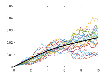
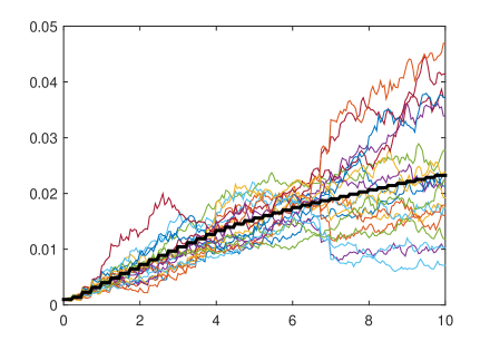
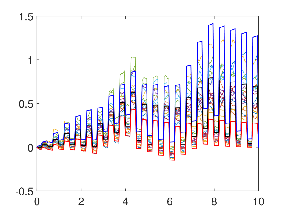
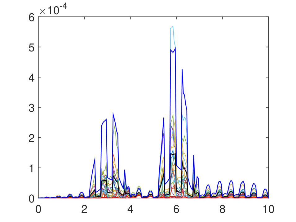
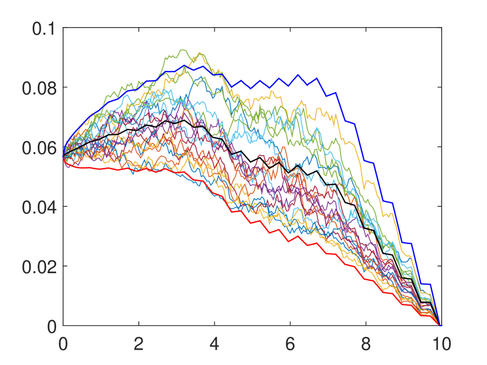
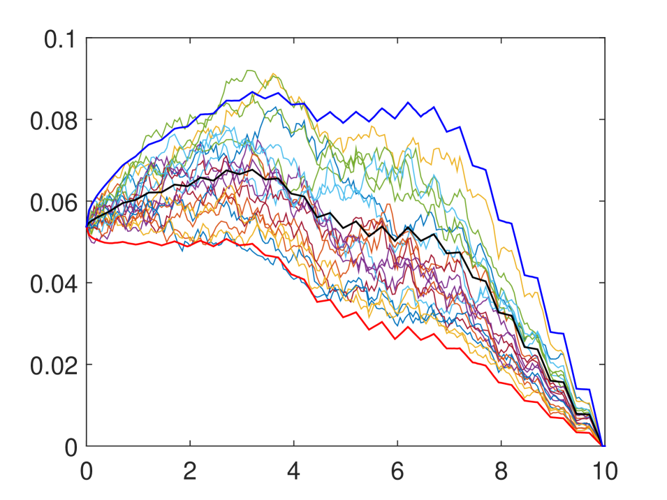
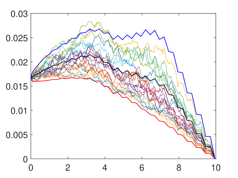
The requirements on the interpolating function 𝒰𝒰\mathpzc U are rather weak, such that even a linear interpolation between the uksubscript𝑢𝑘u_{k}’s corresponding to the maturities Tksubscript𝑇𝑘T_{k}, k𝒦𝑘𝒦k\in\mathcal{K}, can be used. However looking at equations (4.6)–(4.7) for the dynamics of the short rate process r𝑟r, we can immediately observe that jumps will occur at fixed times, the maturities Tksubscript𝑇𝑘T_{k}, if 𝒰𝒰\mathpzc U is not continuously differentiable. A more sophisticated, but still arbitrary, choice for an interpolating function are cubic splines, i.e. piecewise polynomials of degree three, which are continuously differentiable and thus do not lead to deterministic discontinuities; see Figure 4.1 for an illustration.

The next corollary is an immediate consequence of Lemma 4.5 and the fact that X𝑋X is stochastically continuous.

Refer to caption
Refer to caption
Figure 4.1. 20 sample paths of the short rate when X𝑋X is the 1D CIR process, together with the mean as a function of time (computed over 105superscript10510^{5} paths). Left panel: using a cubic spline nterpolation of (uk)subscript𝑢𝑘\left(u_{k}\right) to obtain 𝒰𝒰\mathpzc{U}. Right panel: using a linear interpolation.
Corollary 4.8.

Let 𝒰𝒰\mathpzc U be a continuously differentiable interpolating function, i.e. 𝒰𝒞1(,0𝒹)𝒰superscript𝒞1superscriptsubscriptabsent0𝒹\mathpzc U\in C^{1}\left(\mathbb{R},\mathbb{R}_{\geqslant 0}^{d}\right), and consider the continuous tenor extension of the affine LIBOR model (X,𝒳,TN,u,v)𝑋𝒳subscript𝑇𝑁𝑢𝑣(X,\mathcal{X},T_{N},u,v). Then the short rate process r𝑟r is stochastically continuous.

However, even when the interpolating function is continuously differentiable there can be sources of undesirable behaviour of the short rate inhereted from the sequence (uk)subscript𝑢𝑘(u_{k}) itself (which is not unique unless d=1𝑑1d=1; cf. Remark 3.8). Consider, for example, the following ‘diagonal’ structure for (uk)subscript𝑢𝑘(u_{k}), which is similar to the one employed by Grbac et al. (2015) to model independence between rates of different maturities:

uN=(000)uN1=(00u¯N)uN2=(0u¯N1u¯N)u1=(u¯1u¯N1u¯N)u0=(u¯0u¯N1u¯N)\begin{array}[t]{cccccc}u_{N}&=&(0&\cdots&0&0)\\ u_{N-1}&=&(0&\reflectbox{$\ddots$}&0&\bar{u}_{N})\\ u_{N-2}&=&(0&\reflectbox{$\ddots$}&\bar{u}_{N-1}&\bar{u}_{N})\\ &&\vdots&\reflectbox{$\ddots$}&\vdots&\vdots\\ u_{1}&=&(\bar{u}_{1}&\cdots&\bar{u}_{N-1}&\bar{u}_{N})\\ u_{0}&=&(\bar{u}_{0}&\cdots&\bar{u}_{N-1}&\bar{u}_{N})\end{array}

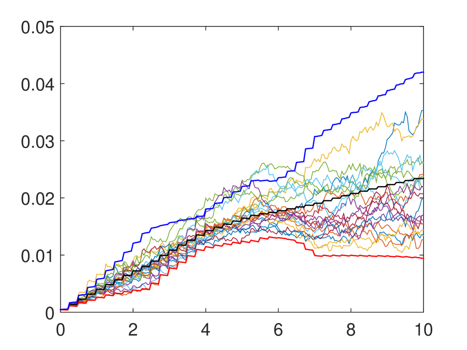
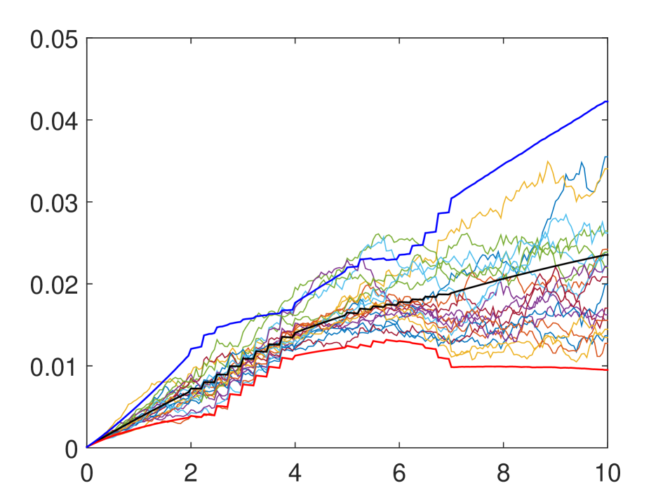
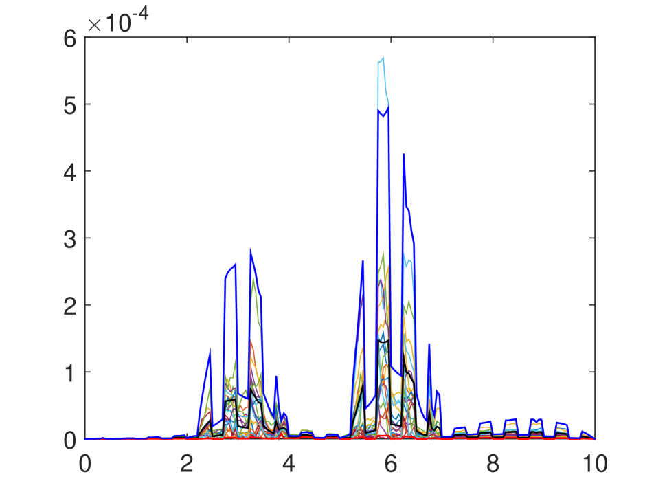
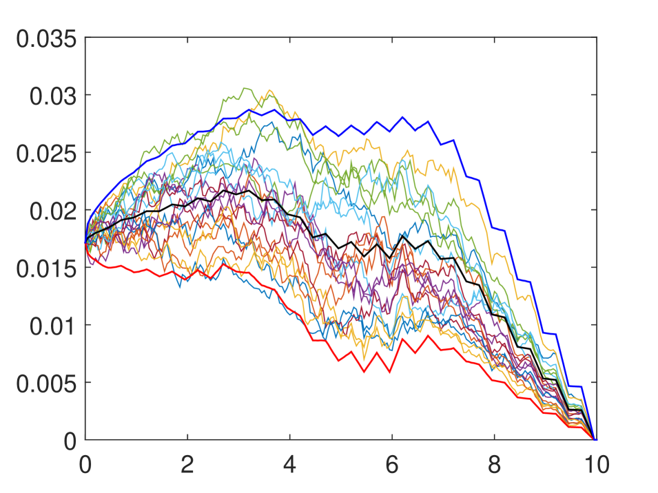
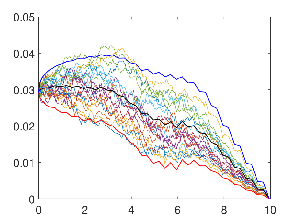
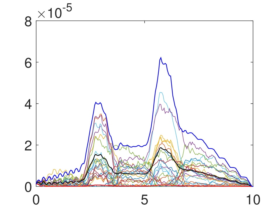
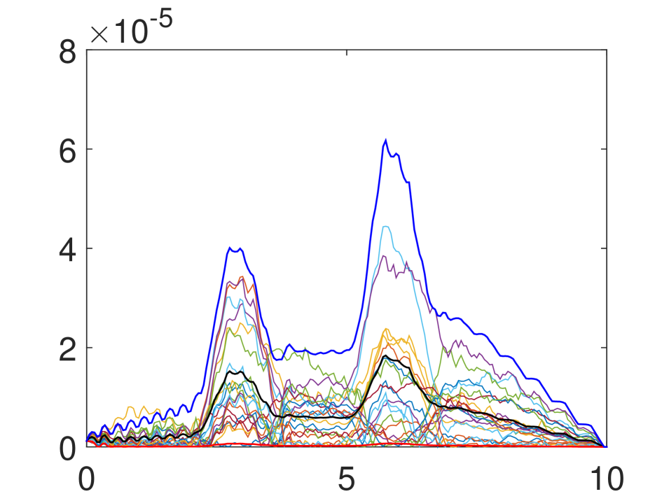
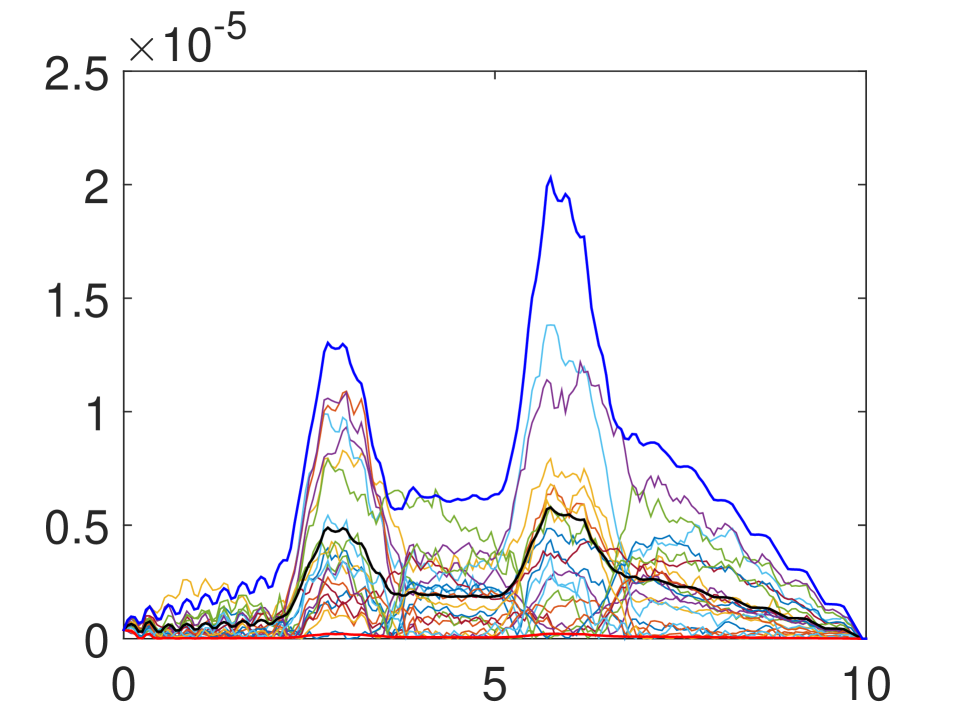
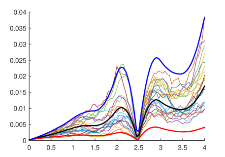
with u¯i0subscript¯𝑢𝑖subscriptabsent0\bar{u}_{i}\in\mathbb{R}_{\geqslant 0}, for 1iN1𝑖𝑁1\leq i\leq N. The only paths that can be used to interpolate in this case are the ones connecting the elements uksubscript𝑢𝑘u_{k} and uk+1subscript𝑢𝑘1u_{k+1} of the sequence (uk)subscript𝑢𝑘(u_{k}) via straight lines, otherwise the interpolating function will not be component-wise decreasing. Hence, any interpolating function maps onto a non-smooth manifold. Then, requiring that the interpolating function is continuously differentiability (in time) will lead to a short rate that drops to zero at every Tksubscript𝑇𝑘T_{k}, k𝒦𝑘𝒦k\in\mathcal{K}, since the derivative of the interpolating function will equal zero at each Tksubscript𝑇𝑘T_{k}; see again (4.6) and (4.7), and the illustration in Figure 4.2.
Refer to caption
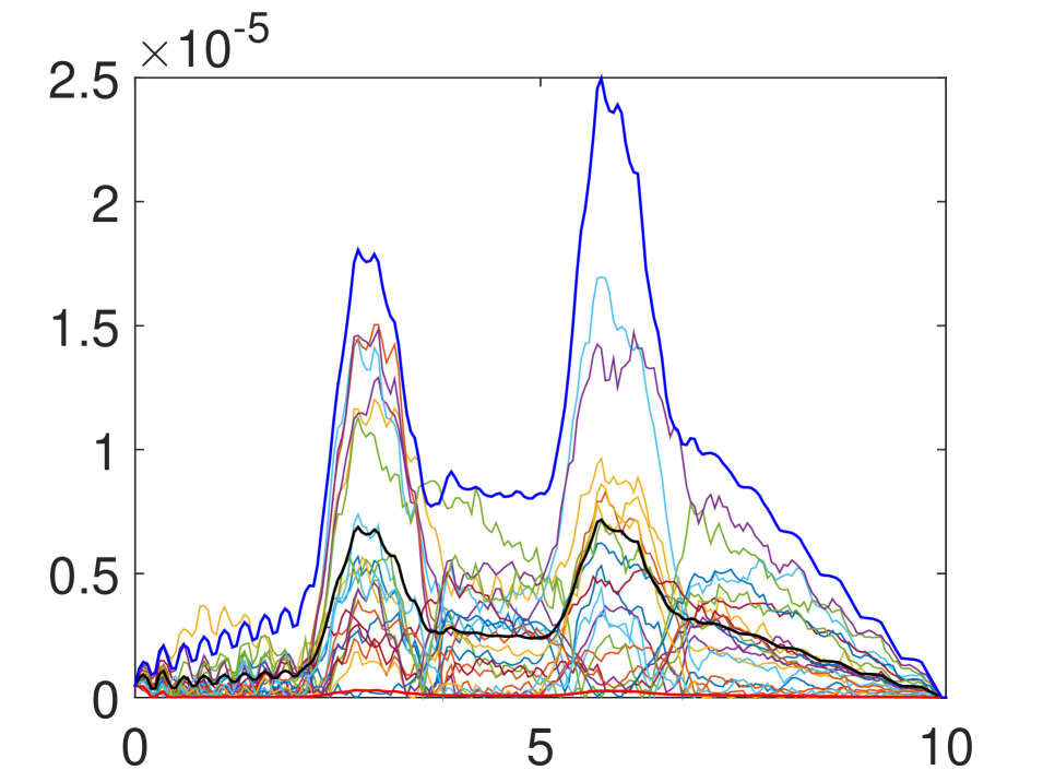
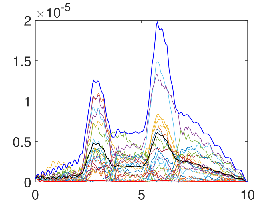
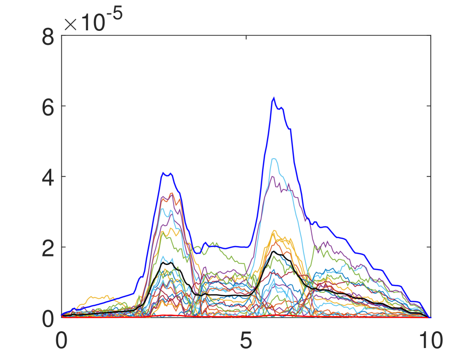
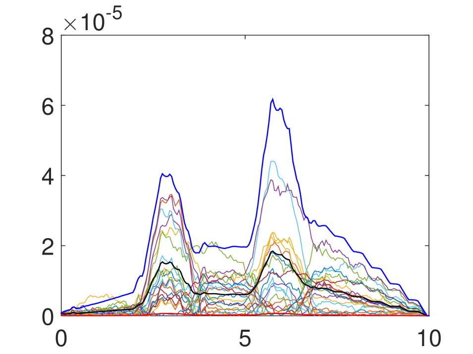
Figure 4.2. 20 sample paths of the short rate together with the 2.5/97.5 percentiles induced by a diagonal structure and a continuously differentiable interpolating function.

We would like in the sequel to provide conditions such that the short rate resulting from a continuous tenor extension of an affine LIBOR model exhibits ‘reasonable’ behavior, in the sense that it neither jumps at fixed times, nor drops to zero at each maturity date. Moreover, we would like to identify a method for choosing an interpolating function that removes the arbitrariness from this choice. A condition for the former is that the sequence (uk)k𝒦subscriptsubscript𝑢𝑘𝑘𝒦(u_{k})_{k\in\mathcal{K}} lies on a smooth manifold. Regarding the latter, we could require that a continuum of bond prices are fitted as well. These two together lead to a uniquely defined, continuously differentiable interpolating function.

Example 4.9.

Let (X,𝒳,TN,u,v)𝑋𝒳subscript𝑇𝑁𝑢𝑣(X,\mathcal{X},T_{N},u,v) be an affine LIBOR model and assume that the sequence (uk)k𝒦subscriptsubscript𝑢𝑘𝑘𝒦(u_{k})_{k\in\mathcal{K}} admits an interpolating function 𝒰^^𝒰\hat{\mathpzc{U}} that maps onto a smooth manifold ={𝒰^(t);t[0,TN]}^𝒰𝑡𝑡0subscript𝑇𝑁\mathscr{M}=\left\{\hat{\mathpzc U}(t);t\in\left[0,T_{N}\right]\right\}. Moreover, let f~(0,):[0,TN]0:~𝑓00subscript𝑇𝑁subscriptabsent0\tilde{f}(0,\cdot)\colon[0,T_{N}]\rightarrow\mathbb{R}_{\geqslant 0} be an initial forward curve—belonging e.g. to the Nelson–Siegel or Svensson family—that is consistent with the initial bond prices, i.e.

B(0,Tk)=exp(0Tkf~(0,s)ds).𝐵0subscript𝑇𝑘superscriptsubscript0subscript𝑇𝑘~𝑓0𝑠differential-d𝑠\displaystyle B(0,T_{k})=\exp\left(-\int_{0}^{T_{k}}\tilde{f}(0,s)\mathrm{d}s\right). (4.13)

Then, we can find an interpolating function 𝒰𝒰\mathpzc U such that the continuous-tenor extended affine LIBOR model fits the given initial forward curve f~~𝑓\tilde{f}. In order to achieve this, the interpolating function 𝒰𝒰\mathpzc{U} should satisfy the following:

ϕTN(𝒰(𝒯))+ψ𝒯𝒩(𝒰(𝒯)),𝒳0=𝒯𝒯𝒩𝒻~(0,𝓈)d𝓈 and 𝒰(𝒯)formulae-sequencesubscriptitalic-ϕsubscript𝑇𝑁𝒰𝒯subscript𝜓subscript𝒯𝒩𝒰𝒯subscript𝒳0superscriptsubscript𝒯subscript𝒯𝒩~𝒻0𝓈differential-d𝓈 and 𝒰𝒯\displaystyle\phi_{T_{N}}\big{(}\mathpzc{U(T)}\big{)}+\big{\langle}\psi_{T_{N}}\big{(}\mathpzc{U(T)}\big{)},X_{0}\big{\rangle}=\int_{\mathpzc T}^{T_{N}}\tilde{f}(0,s)\mathrm{d}s\quad\mbox{ and }\quad\mathpzc{U(T)}\in\mathscr{M} (4.14)

for all 𝒯[0,𝒯𝒩]𝒯0subscript𝒯𝒩\mathpzc T\in[0,T_{N}]. This equation follows directly from the requirement that (4.13) holds for all 𝒯[0,𝒯𝒩]𝒯0subscript𝒯𝒩\mathpzc T\in[0,T_{N}], together with (4.2)–(4.3) and Remark 4.2. Moreover, the dynamics of the instantaneous forward rate are provided by (4.6)–(4.7) for all 𝒯[0,𝒯𝒩]𝒯0subscript𝒯𝒩\mathpzc{T}\in[0,T_{N}], and satisfy the initial condition f(0,𝒯)=f~(0,𝒯)𝑓0𝒯~𝑓0𝒯f\left(0,\mathpzc{T}\right)=\tilde{f}\left(0,\mathpzc{T}\right).

The curve fitting problem in (4.14) can be solved analogously to the problem of fitting the sequence (uk)subscript𝑢𝑘(u_{k}) to an initial term structure of bond prices; compare with Proposition 6.1 in Keller-Ressel et al. (2013) and the corresponding proof. The resulting interpolating function is then differentiable with respect to time, as the following result shows.

Proposition 4.10.

Let (X,𝒳,TN,u,v)𝑋𝒳subscript𝑇𝑁𝑢𝑣(X,\mathcal{X},T_{N},u,v) be a multiple curve affine LIBOR model, assume that f~(0,):[0,TN]0:~𝑓00subscript𝑇𝑁subscriptabsent0\tilde{f}(0,\cdot):[0,T_{N}]\to\mathbb{R}_{\geqslant 0} is continuous and that (uk)k𝒦subscriptsubscript𝑢𝑘𝑘𝒦(u_{k})_{k\in\mathcal{K}} allows for an interpolating function that maps onto a C1superscript𝐶1C^{1}-manifold T0dsubscript𝑇subscriptsuperscript𝑑absent0\mathscr{M}\subseteq\mathcal{I}_{T}\cap\mathbb{R}^{d}_{\geqslant 0}. Then, there exists a unique continuously differentiable interpolating function 𝒰:[0,𝒯𝒩]:𝒰0subscript𝒯𝒩\mathpzc U\colon[0,T_{N}]\rightarrow\mathscr{M} satisfying (4.14).

Proof.

This statement is an easy consequence of the implicit function theorem, where the differentiability of ϕitalic-ϕ\phi and ψ𝜓\psi in space and time as well as their order preserving property (cf. Lemma 2.1) are used. Indeed, the function

G(t,u)=ϕTN(u)+ψTN(u),X0tTNf~(0,s)ds𝐺𝑡𝑢subscriptitalic-ϕsubscript𝑇𝑁𝑢subscript𝜓subscript𝑇𝑁𝑢subscript𝑋0subscriptsuperscriptsubscript𝑇𝑁𝑡~𝑓0𝑠differential-d𝑠G\left(t,u\right)=\phi_{T_{N}}\left(u\right)+\left\langle\psi_{T_{N}}\left(u\right),X_{0}\right\rangle-\int^{T_{N}}_{t}\tilde{f}\left(0,s\right)\mathrm{d}s

is continuously differentiable in t[0,TN]𝑡0subscript𝑇𝑁t\in[0,T_{N}] and uT𝑢subscript𝑇u\in\mathcal{I}_{T}. Let (Uα,gα)α𝒜subscriptsubscript𝑈𝛼subscript𝑔𝛼𝛼𝒜\left(U_{\alpha},g_{\alpha}\right)_{\alpha\in\mathpzc{A}} be an atlas for the C1superscript𝐶1C^{1}-manifold \mathscr{M}, where 𝒜𝒜\mathpzc{A} is a finite index set, (Uα)α𝒜subscriptsubscript𝑈𝛼𝛼𝒜\left(U_{\alpha}\right)_{\alpha\in\mathpzc{A}} is an open covering of \mathscr{M} and gα:UαIα:subscript𝑔𝛼subscript𝑈𝛼subscript𝐼𝛼g_{\alpha}:U_{\alpha}\rightarrow I_{\alpha}\subseteq\mathbb{R} is a C1superscript𝐶1C^{1}-homeomorphism. Define G:[0,TN]×Iα:superscript𝐺0subscript𝑇𝑁subscript𝐼𝛼G^{\star}\colon[0,T_{N}]\times I_{\alpha}\rightarrow\mathbb{R} by (t,x)G(t,gα1(x))maps-to𝑡𝑥𝐺𝑡subscriptsuperscript𝑔1𝛼𝑥\left(t,x\right)\mapsto G\left(t,g^{-1}_{\alpha}\left(x\right)\right). By the (strict-)order preserving property of ϕitalic-ϕ\phi and ψ𝜓\psi we know that the partial derivative xG(t,x)𝑥superscript𝐺𝑡𝑥\frac{\partial}{\partial x}G^{\star}\left(t,x\right) is not zero, hence by a compactness argument there exists a unique continuously differentiable function x:[0,TN]:𝑥0subscript𝑇𝑁x\colon[0,T_{N}]\rightarrow\mathbb{R} such that G(t,x(t))=0superscript𝐺𝑡𝑥𝑡0G^{\star}\left(t,x\left(t\right)\right)=0 for all t[0,TN]𝑡0subscript𝑇𝑁t\in[0,T_{N}]. The interpolating function is then given by 𝒰(𝓉)α1(𝓍(𝓉))𝒰𝓉subscriptsuperscript1𝛼𝓍𝓉\mathpzc{U}\left(t\right)\coloneqq g^{-1}_{\alpha}(x(t)). ∎

Remark 4.11.

Figure 4.1 reveals another interesting behavior of the short rate implied by an affine LIBOR model. In particular, there exists a lower bound for the short rate that is greater than zero. Indeed, since the state space of our driving affine process is 0dsuperscriptsubscriptabsent0𝑑\mathbb{R}_{\geqslant 0}^{d}, we have that rtptsubscript𝑟𝑡subscript𝑝𝑡r_{t}\geq p_{t}, which is greater than zero as ϕitalic-ϕ\phi is strictly order preserving and u𝑢u is decreasing. A similar phenomenon was already observed in the discrete tenor model for the LIBOR rate, compare with Keller-Ressel et al. (2013, Rem. 6.4).

5. Computation of XVA in affine LIBOR models

The quoted price of a derivative product in pre-crisis markets was equal to its discounted expected payoff (under a martingale measure), since counterparties were considered default-free, there was abundance of liquidity in the markets, and other frictions were also negligible. In post-crisis markets however these assumptions have been challenged; in particular, counterparty credit risk has emerged as the natural form of default risk, there is shortage of liquidity in financial markets, while other frictions have also gained importance. These facts have thus to be factored into the quoted price. One way to do that, is to compute first the so-called ‘clean’ price of the derivative, which equals its discounted expected payoff (under a martingale measure), and then add to it several value adjustments, collectively abbreviated as XVA, that reflect counterparty credit risk, liquidity costs, etc. We refer to Brigo et al. (2013), Crépey (2015a, b), Crépey and Bielecki (2014) and Bichuch et al. (2016) among others for more details on XVA.

5.1. Clean valuation

This section reviews basis swaps and provides formulas for their clean price in affine LIBOR models with multiple curves. The clean valuation of caps, swaptions and basis swaptions in these models is extensively studied in Grbac et al. (2015).

The typical example of an interest rate swap is where a floating rate is exchanged for a fixed rate; see, e.g., Musiela and Rutkowski (2005, §9.4). The appearance of significant spreads between rates of different tenors has given rise to a new kind of interest rate swap, called basis swap, where two streams of floating payments linked to underlying rates of different tenors are exchanged. As an example, in a 3M-6M basis swap linked to the LIBOR, the 3-month LIBOR is paid quarterly and the 6-month LIBOR is received semiannually.

Let 𝒯p1q1x1={Tp1x1,,Tq1x1}superscriptsubscript𝒯subscript𝑝1subscript𝑞1subscript𝑥1superscriptsubscript𝑇subscript𝑝1subscript𝑥1superscriptsubscript𝑇subscript𝑞1subscript𝑥1\mathcal{T}_{p_{1}q_{1}}^{x_{1}}=\left\{T_{p_{1}}^{x_{1}},\dots,T_{q_{1}}^{x_{1}}\right\} and 𝒯p2q2x2={Tp2x2,,Tq2x2}superscriptsubscript𝒯subscript𝑝2subscript𝑞2subscript𝑥2superscriptsubscript𝑇subscript𝑝2subscript𝑥2superscriptsubscript𝑇subscript𝑞2subscript𝑥2\mathcal{T}_{p_{2}q_{2}}^{x_{2}}=\left\{T_{p_{2}}^{x_{2}},\dots,T_{q_{2}}^{x_{2}}\right\} denote two tenor structures, where Tp1x1=Tp2x2superscriptsubscript𝑇subscript𝑝1subscript𝑥1superscriptsubscript𝑇subscript𝑝2subscript𝑥2T_{p_{1}}^{x_{1}}=T_{p_{2}}^{x_{2}}, Tq1x1=Tq2x2superscriptsubscript𝑇subscript𝑞1subscript𝑥1superscriptsubscript𝑇subscript𝑞2subscript𝑥2T_{q_{1}}^{x_{1}}=T_{q_{2}}^{x_{2}} and 𝒯p2q2x2𝒯p1q1x1superscriptsubscript𝒯subscript𝑝2subscript𝑞2subscript𝑥2superscriptsubscript𝒯subscript𝑝1subscript𝑞1subscript𝑥1\mathcal{T}_{p_{2}q_{2}}^{x_{2}}\subset\mathcal{T}_{p_{1}q_{1}}^{x_{1}}. Consider a basis swap that is initiated at Tp1x1=Tp2x2superscriptsubscript𝑇subscript𝑝1subscript𝑥1superscriptsubscript𝑇subscript𝑝2subscript𝑥2T_{p_{1}}^{x_{1}}=T_{p_{2}}^{x_{2}}, with the first payments due at Tp1+1x1superscriptsubscript𝑇subscript𝑝11subscript𝑥1T_{p_{1}+1}^{x_{1}} and Tp2+1x2superscriptsubscript𝑇subscript𝑝21subscript𝑥2T_{p_{2}+1}^{x_{2}} respectively. In order to reflect the possible discrepancy between the floating rates at initiation, the interest rate L(Ti1x1,Tix1)𝐿superscriptsubscript𝑇𝑖1subscript𝑥1superscriptsubscript𝑇𝑖subscript𝑥1L\left(T_{i-1}^{x_{1}},T_{i}^{x_{1}}\right) corresponding to the shorter tenor length x1subscript𝑥1x_{1} is replaced by L(Ti1x1,Tix1)+S𝐿superscriptsubscript𝑇𝑖1subscript𝑥1superscriptsubscript𝑇𝑖subscript𝑥1𝑆L\left(T_{i-1}^{x_{1}},T_{i}^{x_{1}}\right)+S for a fixed S𝑆S, which is called the basis swap spread. The time-r𝑟r value of a basis swap with notional amount normalized to 111, for 0rTp1x10𝑟superscriptsubscript𝑇subscript𝑝1subscript𝑥10\leq r\leq T_{p_{1}}^{x_{1}}, is given by

𝔹𝕊r(S,𝒯p1q1x1,𝒯p2q2x2)=i=p2+1q2δx2B(r,Tix2)𝔼ix2[L(Ti1x2,Tix2)|r]i=p1+1q1δx1B(r,Tix1)𝔼ix1[L(Ti1x1,Tix1)+S|r]=i=p2+1q2δx2B(r,Tix2)Lix2(r)i=p1+1q1δx1B(r,Tix1)(Lix1(r)+S).𝔹subscript𝕊𝑟𝑆superscriptsubscript𝒯subscript𝑝1subscript𝑞1subscript𝑥1superscriptsubscript𝒯subscript𝑝2subscript𝑞2subscript𝑥2superscriptsubscript𝑖subscript𝑝21subscript𝑞2subscript𝛿subscript𝑥2𝐵𝑟superscriptsubscript𝑇𝑖subscript𝑥2superscriptsubscript𝔼𝑖subscript𝑥2delimited-[]conditional𝐿superscriptsubscript𝑇𝑖1subscript𝑥2superscriptsubscript𝑇𝑖subscript𝑥2subscript𝑟superscriptsubscript𝑖subscript𝑝11subscript𝑞1subscript𝛿subscript𝑥1𝐵𝑟superscriptsubscript𝑇𝑖subscript𝑥1superscriptsubscript𝔼𝑖subscript𝑥1delimited-[]𝐿superscriptsubscript𝑇𝑖1subscript𝑥1superscriptsubscript𝑇𝑖subscript𝑥1conditional𝑆subscript𝑟superscriptsubscript𝑖subscript𝑝21subscript𝑞2subscript𝛿subscript𝑥2𝐵𝑟superscriptsubscript𝑇𝑖subscript𝑥2superscriptsubscript𝐿𝑖subscript𝑥2𝑟superscriptsubscript𝑖subscript𝑝11subscript𝑞1subscript𝛿subscript𝑥1𝐵𝑟superscriptsubscript𝑇𝑖subscript𝑥1superscriptsubscript𝐿𝑖subscript𝑥1𝑟𝑆\mathbb{BS}_{r}\left(S,\mathcal{T}_{p_{1}q_{1}}^{x_{1}},\mathcal{T}_{p_{2}q_{2}}^{x_{2}}\right)=\sum_{i=p_{2}+1}^{q_{2}}\delta_{x_{2}}B\left(r,T_{i}^{x_{2}}\right)\mathds{E}_{i}^{x_{2}}\left[\left.L\left(T_{i-1}^{x_{2}},T_{i}^{x_{2}}\right)\right|\mathcal{F}_{r}\right]\\ -\sum_{i=p_{1}+1}^{q_{1}}\delta_{x_{1}}B\left(r,T_{i}^{x_{1}}\right)\mathds{E}_{i}^{x_{1}}\left[\left.L\left(T_{i-1}^{x_{1}},T_{i}^{x_{1}}\right)+S\right|\mathcal{F}_{r}\right]\\ =\sum_{i=p_{2}+1}^{q_{2}}\delta_{x_{2}}B(r,T_{i}^{x_{2}})L_{i}^{x_{2}}(r)-\sum_{i=p_{1}+1}^{q_{1}}\delta_{x_{1}}B(r,T_{i}^{x_{1}})\left(L_{i}^{x_{1}}(r)+S\right).

The fair basis swap spread Sr(𝒯p1q1x1,𝒯p2q2x2)subscript𝑆𝑟superscriptsubscript𝒯subscript𝑝1subscript𝑞1subscript𝑥1superscriptsubscript𝒯subscript𝑝2subscript𝑞2subscript𝑥2S_{r}(\mathcal{T}_{p_{1}q_{1}}^{x_{1}},\mathcal{T}_{p_{2}q_{2}}^{x_{2}}) is then computed such that the value of the swap at inception is zero, i.e. 𝔹𝕊r(S,𝒯p1q1x1,𝒯p2q2x2)=0𝔹subscript𝕊𝑟𝑆superscriptsubscript𝒯subscript𝑝1subscript𝑞1subscript𝑥1superscriptsubscript𝒯subscript𝑝2subscript𝑞2subscript𝑥20\mathbb{BS}_{r}(S,\mathcal{T}_{p_{1}q_{1}}^{x_{1}},\mathcal{T}_{p_{2}q_{2}}^{x_{2}})=0 for 0rTp1x10𝑟superscriptsubscript𝑇subscript𝑝1subscript𝑥10\leq r\leq T_{p_{1}}^{x_{1}}. Hence, the fair spread is given by

Sr(𝒯p1q1x1,𝒯p2q2x2)=i=p2+1q2δx2B(r,Tix2)Lix2(r)i=p1+1q1δx1B(r,Tix1)Lix1(r)i=p1+1q1δx1B(r,Tix1).subscript𝑆𝑟superscriptsubscript𝒯subscript𝑝1subscript𝑞1subscript𝑥1superscriptsubscript𝒯subscript𝑝2subscript𝑞2subscript𝑥2superscriptsubscript𝑖subscript𝑝21subscript𝑞2subscript𝛿subscript𝑥2𝐵𝑟superscriptsubscript𝑇𝑖subscript𝑥2superscriptsubscript𝐿𝑖subscript𝑥2𝑟superscriptsubscript𝑖subscript𝑝11subscript𝑞1subscript𝛿subscript𝑥1𝐵𝑟superscriptsubscript𝑇𝑖subscript𝑥1superscriptsubscript𝐿𝑖subscript𝑥1𝑟superscriptsubscript𝑖subscript𝑝11subscript𝑞1subscript𝛿subscript𝑥1𝐵𝑟superscriptsubscript𝑇𝑖subscript𝑥1\displaystyle S_{r}(\mathcal{T}_{p_{1}q_{1}}^{x_{1}},\mathcal{T}_{p_{2}q_{2}}^{x_{2}})=\frac{\sum_{i=p_{2+1}}^{q_{2}}\delta_{x_{2}}B(r,T_{i}^{x_{2}})L_{i}^{x_{2}}(r)-\sum_{i=p_{1}+1}^{q_{1}}\delta_{x_{1}}B(r,T_{i}^{x_{1}})L_{i}^{x_{1}}(r)}{\sum_{i=p_{1}+1}^{q_{1}}\delta_{x_{1}}B(r,T_{i}^{x_{1}})}.

Moreover, the time-t𝑡t value of the basis swap, for t[Tp1x1,Tq2x2]𝑡superscriptsubscript𝑇subscript𝑝1subscript𝑥1superscriptsubscript𝑇subscript𝑞2subscript𝑥2t\in\left[T_{p_{1}}^{x_{1}},T_{q_{2}}^{x_{2}}\right], using (3.8) and (4.1), takes the form:

𝔹𝕊t(Sr,𝒯p1q1x1,𝒯p2q2x2)𝔹subscript𝕊𝑡subscript𝑆𝑟superscriptsubscript𝒯subscript𝑝1subscript𝑞1subscript𝑥1superscriptsubscript𝒯subscript𝑝2subscript𝑞2subscript𝑥2\displaystyle\mathbb{BS}_{t}\left(S_{r},\mathcal{T}_{p_{1}q_{1}}^{x_{1}},\mathcal{T}_{p_{2}q_{2}}^{x_{2}}\right) =1Mt𝒰(𝓉)i=t2q2(Mtvi1x2Mtuix2)absent1superscriptsubscript𝑀𝑡𝒰𝓉superscriptsubscript𝑖subscript𝑡2subscript𝑞2superscriptsubscript𝑀𝑡superscriptsubscript𝑣𝑖1subscript𝑥2superscriptsubscript𝑀𝑡superscriptsubscript𝑢𝑖subscript𝑥2\displaystyle=\frac{1}{M_{t}^{\mathpzc U(t)}}\sum_{i=\lceil t\rceil_{2}}^{q_{2}}\left(M_{t}^{v_{i-1}^{x_{2}}}-M_{t}^{u_{i}^{x_{2}}}\right)
1Mt𝒰(𝓉)i=t1q1(Mtvi1x1Mtuix1(1δx1Sr)),1superscriptsubscript𝑀𝑡𝒰𝓉superscriptsubscript𝑖subscript𝑡1subscript𝑞1superscriptsubscript𝑀𝑡superscriptsubscript𝑣𝑖1subscript𝑥1superscriptsubscript𝑀𝑡superscriptsubscript𝑢𝑖subscript𝑥11subscript𝛿subscript𝑥1subscript𝑆𝑟\displaystyle\quad-\frac{1}{M_{t}^{\mathpzc U(t)}}\sum_{i=\lceil t\rceil_{1}}^{q_{1}}\left(M_{t}^{v_{i-1}^{x_{1}}}-M_{t}^{u_{i}^{x_{1}}}\left(1-\delta_{x_{1}}S_{r}\right)\right), (5.1)

where Sr=Sr(𝒯p1q1x1,𝒯p2q2x2)subscript𝑆𝑟subscript𝑆𝑟superscriptsubscript𝒯subscript𝑝1subscript𝑞1subscript𝑥1superscriptsubscript𝒯subscript𝑝2subscript𝑞2subscript𝑥2S_{r}=S_{r}\left(\mathcal{T}_{p_{1}q_{1}}^{x_{1}},\mathcal{T}_{p_{2}q_{2}}^{x_{2}}\right), for r[0,Tp1x1]𝑟0superscriptsubscript𝑇subscript𝑝1subscript𝑥1r\in[0,T_{p_{1}}^{x_{1}}] being the date of inception, while ti=min{k𝒦xi:t<Tkxi}subscript𝑡𝑖:𝑘superscript𝒦subscript𝑥𝑖𝑡superscriptsubscript𝑇𝑘subscript𝑥𝑖\lceil t\rceil_{i}=\min\left\{k\in\mathcal{K}^{x_{i}}:t<T_{k}^{x_{i}}\right\}.

Remark 5.1.

Basis swaps are post-crisis financial products, which can only be priced in models accounting for the multiple curve nature of interest rates. In a single curve model, the price of a basis swap is zero; cf. Crépey et al. (2012, p. 181)

5.2. XVA equations

The pricing formulas in the previous subsection reflect valuation in an environment without counterparty credit risk, funding constraints and other market frictions. In order to include the latter into the pricing framework, several value adjustments have been introduced: credit and debt valuation adjustment (CVA and DVA), liquidity valuation adjustment (LVA), as well as replacement cost (RC), among others. The various valuation adjustments are typically abbreviated by XVA, while we will refer to their sum as the total valuation adjustment (TVA), i.e.

TVA=CVA+DVA+LVA+RC;TVACVADVALVARC\mbox{TVA}=\mbox{CVA}+\mbox{DVA}+\mbox{LVA}+\mbox{RC};

see also Crépey et al. (2013). Our approach to the computation of TVA follows closely the work of Crépey (2015a, b).

We consider two counterparties, called a bank and an investor in the sequel, that are both defaultable, and denote by τbsubscript𝜏𝑏\tau_{b} the default time of the bank, by τisubscript𝜏𝑖\tau_{i} the default time of the investor, while we set τ=τbτiT𝜏subscript𝜏𝑏subscript𝜏𝑖𝑇\tau=\tau_{b}\wedge\tau_{i}\wedge T. The default intensities of τb,τisubscript𝜏𝑏subscript𝜏𝑖\tau_{b},\tau_{i} and τ𝜏\tau are denoted γb,γisubscript𝛾𝑏subscript𝛾𝑖\gamma_{b},\gamma_{i} and γ𝛾\gamma, respectively. We also consider the ‘full model’ filtration 𝔾𝔾\mathbb{G}, which is given by 𝔽𝔽\mathbb{F} enlarged by the natural filtrations of the default times τbsubscript𝜏𝑏\tau_{b} and τisubscript𝜏𝑖\tau_{i}, and assume that the immersion hypothesis holds, that is, every 𝔽𝔽\mathbb{F}-martingale stopped at τ𝜏\tau is a 𝔾𝔾\mathbb{G}-martingale.

The TVA can be viewed as the price of a dividend paying option on the debt of the bank to the investor, paying off at the first-to-default time τ𝜏\tau. Here, we have implicitly adopted the point of view of the bank. The TVA from the point of view of the investor is similar, but not identical, due to e.g. different funding conditions. The effective conclusion of Crépey (2015b) is that the TVA in the setting described above can be computed in a ‘pre-default’ framework, where the default risk of the counterparties appears only through the default intensities; see, in particular, Section 3 therein. More specifically, the TVA ΘΘ\Theta is the solution of the following BSDE under a martingale measure \mathds{P}:

Θt=𝔼t(tTgs(rs,Ps,Θs)ds),t[0,T],formulae-sequencesubscriptΘ𝑡subscript𝔼𝑡superscriptsubscript𝑡𝑇subscript𝑔𝑠subscript𝑟𝑠subscript𝑃𝑠subscriptΘ𝑠differential-d𝑠𝑡0𝑇\displaystyle\Theta_{t}=\mathds{E}_{t}\left(\int_{t}^{T}g_{s}\left(r_{s},P_{s},\Theta_{s}\right)\mathrm{d}s\right),\quad t\in[0,T], (5.2)

where r𝑟r denotes the short rate process, P𝑃P the clean price process and g𝑔g the TVA coefficient. The overall price of the contract for the bank, in other words, the cost of the hedge incorporating the various risks, is then given by the diffference between the clean price and the TVA:

Πt=PtΘt,t[0,T].formulae-sequencesubscriptΠ𝑡subscript𝑃𝑡subscriptΘ𝑡𝑡0𝑇\Pi_{t}=P_{t}-\Theta_{t},\quad t\in[0,T].

The TVA coefficient g𝑔g has the following form:

gt(rt,Pt,Θt)+rtΘt=subscript𝑔𝑡subscript𝑟𝑡subscript𝑃𝑡subscriptΘ𝑡subscript𝑟𝑡subscriptΘ𝑡absent\displaystyle\!\!\!\!\!\!\!\!\!\!\!\!\!g_{t}(r_{t},P_{t},\Theta_{t})+r_{t}\Theta_{t}\ =
γti(1ρi)(QtΓt)superscriptsubscript𝛾𝑡𝑖1superscript𝜌𝑖superscriptsubscript𝑄𝑡subscriptΓ𝑡\displaystyle-\gamma_{t}^{i}\left(1-\rho^{i}\right)\left(Q_{t}-\Gamma_{t}\right)^{-} (CVA)
+γtb(1ρb)(QtΓt)+superscriptsubscript𝛾𝑡𝑏1superscript𝜌𝑏superscriptsubscript𝑄𝑡subscriptΓ𝑡\displaystyle+\gamma_{t}^{b}\left(1-\rho^{b}\right)\left(Q_{t}-\Gamma_{t}\right)^{+} (DVA)
+btΓt+b¯tΓt+λt(PtΘtΓt)+λ~t(PtΘtΓt)subscript𝑏𝑡superscriptsubscriptΓ𝑡subscript¯𝑏𝑡superscriptsubscriptΓ𝑡subscript𝜆𝑡superscriptsubscript𝑃𝑡subscriptΘ𝑡subscriptΓ𝑡subscript~𝜆𝑡superscriptsubscript𝑃𝑡subscriptΘ𝑡subscriptΓ𝑡\displaystyle+b_{t}\Gamma_{t}^{+}-\bar{b}_{t}\Gamma_{t}^{-}+\lambda_{t}\left(P_{t}-\Theta_{t}-\Gamma_{t}\right)^{+}-\tilde{\lambda}_{t}\left(P_{t}-\Theta_{t}-\Gamma_{t}\right)^{-} (LVA)
+γt(PtΘtQt),subscript𝛾𝑡subscript𝑃𝑡subscriptΘ𝑡subscript𝑄𝑡\displaystyle+\gamma_{t}\left(P_{t}-\Theta_{t}-Q_{t}\right), (RC)

where λ~t=λ¯tγtb(1𝔯)subscript~𝜆𝑡subscript¯𝜆𝑡superscriptsubscript𝛾𝑡𝑏1𝔯\tilde{\lambda}_{t}=\bar{\lambda}_{t}-\gamma_{t}^{b}(1-\mathfrak{r}), while each line on the right hand side corresponds to one of the four components of the TVA. The parameters in the above equation have the following financial interpretation:

  • γti,γtbsuperscriptsubscript𝛾𝑡𝑖superscriptsubscript𝛾𝑡𝑏\gamma_{t}^{i},\,\gamma_{t}^{b} and γtsubscript𝛾𝑡\gamma_{t} are the default intensities of the investor, the bank and the first to default intensity, respectively.

  • ρi,ρbsuperscript𝜌𝑖superscript𝜌𝑏\rho^{i},\,\rho^{b} are the recovery rates of the investor and the bank to each other, and 𝔯𝔯\mathfrak{r} is the recovery rate of the bank to its unsecured funder (which is a third party that jumps in when the banks’ internal sources of funding have been depleted; this funder is assumed to be risk free).

  • Qtsubscript𝑄𝑡Q_{t} is the value of the contract according to some valuation scheme specified in the credit support annex (CSA), which is a common part in an over-the-counter contract.

  • Γt=Γt+ΓtsubscriptΓ𝑡superscriptsubscriptΓ𝑡superscriptsubscriptΓ𝑡\Gamma_{t}=\Gamma_{t}^{+}-\Gamma_{t}^{-} is the value of the collateral posted by the bank to the investor.

  • bt,b¯tsubscript𝑏𝑡subscript¯𝑏𝑡b_{t},\,\bar{b}_{t} and λt,λ¯tsubscript𝜆𝑡subscript¯𝜆𝑡\lambda_{t},\,\bar{\lambda}_{t} are the spreads over the risk free rate rtsubscript𝑟𝑡r_{t} corresponding to the remuneration of collateral and external lending and borrowing (from the unsecured funder).

The value of the contract Q𝑄Q and of the collateral ΓΓ\Gamma, as well as the funding coefficients b𝑏b and b¯¯𝑏\bar{b} are specified in the CSA of the contract, which is used to mitigate counterparty risk. Different CSA specifications will result in different behavior of the TVA; see Crépey et al. (2013, Sec. 3) for more details and also the next subsection.

Remark 5.2.

The immersion hypothesis implies weak or indirect dependence between the contract and the default times of the involved parties. Therefore not every contract can be priced within the pre-default TVA framework. As interest rate contracts exhibit weak dependence on the default times, this approach is appropriate for our setting; see also Crépey (2015b, Rem. 2.3).

5.3. XVA computation in affine LIBOR models

We are interested now in computing the value adjustments for interest rate derivatives, and focus on basis swaps as a prime example of a post-crisis product. The OIS forward rate and the forward LIBOR rate for each tenor are modeled according to the affine LIBOR models with multiple curves, and the model is calibrated to caplet data; see Grbac et al. (2015, §8) for details on the calibration of affine LIBOR models. An interpolating function is subsequently chosen and the dynamics of the short rate process are derived. Afterwords, the computation of the value adjustments is a straightforward application of the TVA BSDE in (5.2).

This methodology allows us to compute option prices and value adjustments consistently since we only have to calibrate the discrete-tenor affine LIBOR model, while the dynamics of the short rate process, which is essential in the computation of the TVA, follows from the interpolation. In particular, we do not need to introduce and calibrate (or estimate) an ‘exogenous’ model for the short rate, as is done in other approaches. The interpolating function plays thus a crucial role in our methodology, since this is the only ‘free’ ingredient once the affine LIBOR model has been calibrated. At the same time, it introduces an element of model risk, through the different possible choices of interpolating functions. In the sequel, we are going thus to examine the impact of different interpolating functions on the value adjustments.
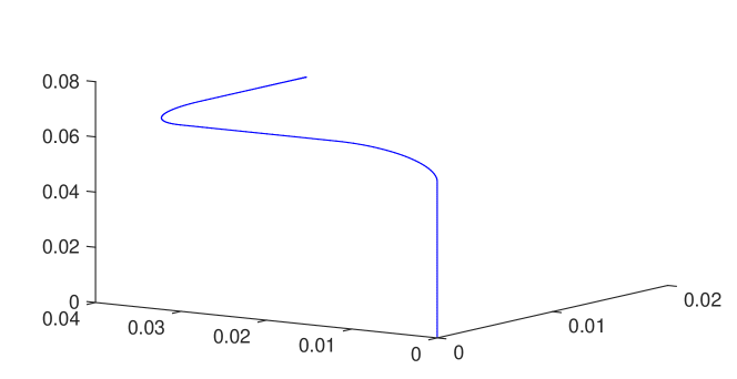
Refer to caption
Figure 5.3. The smooth manifold used for fitting the sequences (uk)subscript𝑢𝑘\left(u_{k}\right) and (vk)subscript𝑣𝑘\left(v_{k}\right).

The data we use for our numerical experiments correspond to the EUR market on 27 May 2013 and were collected from Bloomberg; see also Grbac et al. (2015, §8.4) for more details. The affine LIBOR model with multiple curves was calibrated to caplet data on a 10 year horizon, where the tenor lengths were 3 and 6 months. The driving affine process consists of three independent CIR processes. The sequences (uk)subscript𝑢𝑘(u_{k}) and (vk)subscript𝑣𝑘(v_{k}) were constructed such that they lie on a smooth manifold on T03subscript𝑇subscriptsuperscript3absent0\mathcal{I}_{T}\cap\mathbb{R}^{3}_{\geqslant 0}; see Figure 5.3. In particular, uksubscript𝑢𝑘u_{k} lies on straight lines for k{0,,k1}{k2,,k3}{k4,,N}𝑘0subscript𝑘1subscript𝑘2subscript𝑘3subscript𝑘4𝑁k\in\left\{0,\dots,k_{1}\right\}\cup\left\{k_{2},\dots,k_{3}\right\}\cup\left\{k_{4},\dots,N\right\} and on elliptical segments for k{k1+1,,k21}{k3+1,,k41}𝑘subscript𝑘11subscript𝑘21subscript𝑘31subscript𝑘41k\in\left\{k_{1}+1,\dots,k_{2}-1\right\}\cup\left\{k_{3}+1,\dots,k_{4}-1\right\}. The sequence u𝑢u thus looks as follows:

uN1=(00u¯N1)uk4=(00u¯k4)uk41=(0u~k41u¯k41)uk42=(0u~k42u¯k42)\begin{array}[t]{ccccc}u_{N-1}&=&(0&0&\bar{u}_{N-1})\\ &\vdots&&&\\ u_{k_{4}}&=&(0&0&\bar{u}_{k_{4}}\ \ )\\ u_{k_{4}-1}&=&(0&\tilde{u}_{k_{4}-1}&\bar{u}_{k_{4}-1})\\ u_{k_{4}-2}&=&(0&\tilde{u}_{k_{4}-2}&\bar{u}_{k_{4}-2})\\ &\vdots&&&\\ \end{array}

where u¯j,u~j0subscript¯𝑢𝑗subscript~𝑢𝑗subscriptabsent0\bar{u}_{j},\tilde{u}_{j}\in\mathbb{R}_{\geqslant 0} and satisfy u¯ju¯j+1subscript¯𝑢𝑗subscript¯𝑢𝑗1\bar{u}_{j}\geq\bar{u}_{j+1} and u~ju~j+1subscript~𝑢𝑗subscript~𝑢𝑗1\tilde{u}_{j}\geq\tilde{u}_{j+1} for all relevant j𝒦𝑗𝒦j\in\mathcal{K}; see (3.6) again. The structure of the sequence vxsuperscript𝑣𝑥v^{x} for each tenor x𝑥x is analogous. In other words, short term forward LIBOR rates are driven by all three components of the driving process X𝑋X, medium term rates by two components, while long term rates are only driven by the last component of X𝑋X. Once the manifolds have been constructed, the sequences (uk)subscript𝑢𝑘(u_{k}) and (vk)subscript𝑣𝑘(v_{k}) were obtained by fitting the model to OIS and EURIBOR data from the same date. (Note that in this example we have N=40𝑁40N=40 and we chose k1=9,k2=16,k3=21formulae-sequencesubscript𝑘19formulae-sequencesubscript𝑘216subscript𝑘321k_{1}=9,k_{2}=16,k_{3}=21 and k4=28subscript𝑘428k_{4}=28.)

In order to illustrate the effect of different interpolating functions on the value adjustments, we consider three different specifications for the interpolating function 𝒰𝒰\mathpzc U:

  • (IF1):

    interpolation by fitting an entire forward curve (see Example 4.9);

  • (IF2):

    linear interpolation between the uksubscript𝑢𝑘u_{k}’s;

  • (IF3):

    spline interpolation on sectors where all but one component of the vector uksubscript𝑢𝑘u_{k} are constant in k𝑘k, and linear interpolation in between these sectors (i.e. when the uksubscript𝑢𝑘u_{k}’s lie on curved segments of the manifold).

Let us now turn our attention to the computation of value adjustments. We consider a 3M-6M basis swap on the LIBOR, with inception at t=0𝑡0t=0 and maturity in 10 years. We follow Crépey et al. (2013) and consider five different CSA specifications, provided by

(CSA1):(𝔯,ρb,ρi)=(0.4,0.4,0.4),Q=P,Γ=0,(CSA2):(𝔯,ρb,ρi)=(1,0.4,0.4),Q=P,Γ=0,(CSA3):(𝔯,ρb,ρi)=(1,1,0.4),Q=P,Γ=0,(CSA4):(𝔯,ρb,ρi)=(1,1,0.4),Q=Π,Γ=0,(CSA5):(𝔯,ρb,ρi)=(1,0.4,0.4),Q=P,Γ=Q=P,:subscriptCSA1absentmissing-subexpressionmissing-subexpression𝔯superscript𝜌𝑏superscript𝜌𝑖0.40.40.4𝑄𝑃missing-subexpressionΓ0:subscriptCSA2absentmissing-subexpressionmissing-subexpression𝔯superscript𝜌𝑏superscript𝜌𝑖10.40.4𝑄𝑃missing-subexpressionΓ0:subscriptCSA3absentmissing-subexpressionmissing-subexpression𝔯superscript𝜌𝑏superscript𝜌𝑖110.4𝑄𝑃missing-subexpressionΓ0:subscriptCSA4absentmissing-subexpressionmissing-subexpression𝔯superscript𝜌𝑏superscript𝜌𝑖110.4𝑄Πmissing-subexpressionΓ0:subscriptCSA5absentmissing-subexpressionmissing-subexpression𝔯superscript𝜌𝑏superscript𝜌𝑖10.40.4𝑄𝑃missing-subexpressionΓ𝑄𝑃\begin{array}[]{lcclccl}(\text{CSA}_{1}):&&&\left(\mathfrak{r},\rho^{b},\rho^{i}\right)=\left(0.4,0.4,0.4\right),&Q=P,&&\Gamma=0,\\ (\text{CSA}_{2}):&&&\left(\mathfrak{r},\rho^{b},\rho^{i}\right)=\left(1,0.4,0.4\right),&Q=P,&&\Gamma=0,\\ (\text{CSA}_{3}):&&&\left(\mathfrak{r},\rho^{b},\rho^{i}\right)=\left(1,1,0.4\right),&Q=P,&&\Gamma=0,\\ (\text{CSA}_{4}):&&&\left(\mathfrak{r},\rho^{b},\rho^{i}\right)=\left(1,1,0.4\right),&Q=\Pi,&&\Gamma=0,\\ (\text{CSA}_{5}):&&&\left(\mathfrak{r},\rho^{b},\rho^{i}\right)=\left(1,0.4,0.4\right),&Q=P,&&\Gamma=Q=P,\end{array}

while the default intensities and spreads equal

γb=5%,γi=7%,γ=10%,b=b¯=λ=1.5%andλ¯=4.5%.formulae-sequenceformulae-sequencesuperscript𝛾𝑏percent5formulae-sequencesuperscript𝛾𝑖percent7formulae-sequence𝛾percent10𝑏¯𝑏𝜆percent1.5and¯𝜆percent4.5\gamma^{b}=5\%,\ \gamma^{i}=7\%,\ \gamma=10\%,\ b=\bar{b}=\lambda=1.5\%\quad\text{and}\quad\bar{\lambda}=4.5\%.

The first three CSA specifications correspond to a ‘clean’ recovery scheme without collateralization, since the value of the contract Q𝑄Q equals the clean price and there is no collateral posted. The fourth specification corresponds to a ‘pre-default’ recovery scheme without collateralization, while the last one corresponds to a fully collateralized contract. Moreover, the first specification yields a linear BSDE in the TVA ΘΘ\Theta, which allows to use (forward) Monte Carlo simulations for the computation of the TVA.

The price Ptsubscript𝑃𝑡P_{t} of the basis swap is provided by (5.1) for each t[Tp1x1,Tq2x2]𝑡superscriptsubscript𝑇subscript𝑝1subscript𝑥1superscriptsubscript𝑇subscript𝑞2subscript𝑥2t\in[T_{p_{1}}^{x_{1}},T_{q_{2}}^{x_{2}}], and we can observe that Ptsubscript𝑃𝑡P_{t} is a deterministic transformation of Xtsubscript𝑋𝑡X_{t}. Moreover, the short rate rtsubscript𝑟𝑡r_{t} is a deterministic, affine, transformation of Xtsubscript𝑋𝑡X_{t}; cf. (4.6). Therefore, the TVA coefficient gt(rt,Pt,Θt)subscript𝑔𝑡subscript𝑟𝑡subscript𝑃𝑡subscriptΘ𝑡g_{t}(r_{t},P_{t},\Theta_{t}) is also a deterministic transformation of Xtsubscript𝑋𝑡X_{t}, and we can define a deterministic function g^^𝑔\hat{g} such that

g^(t,Xt,Θt):=gt(rt,Pt,Θt).assign^𝑔𝑡subscript𝑋𝑡subscriptΘ𝑡subscript𝑔𝑡subscript𝑟𝑡subscript𝑃𝑡subscriptΘ𝑡\hat{g}(t,X_{t},\Theta_{t}):=g_{t}(r_{t},P_{t},\Theta_{t}).

In other words, the TVA BSDE is Markovian in this case, and the TVA is also provided by the solution of a semi-linear PDE. In order to compute the TVA for the basis swap numerically, we worked under the spot martingale measure subscript\mathds{P}_{\star}, using a space grid consisting of 105superscript10510^{5} paths and a time grid with n=200𝑛200n=200 steps of step size hh. We applied a backwards regression on the space-time grid, i.e.

Θtln=𝔼[Θtl+1n+hg^(tl+1,Xtl+1n,Θtl+1n)|Xtln] and Θtnn=0,formulae-sequencesuperscriptsubscriptΘsubscript𝑡𝑙𝑛subscript𝔼delimited-[]superscriptsubscriptΘsubscript𝑡𝑙1𝑛conditional^𝑔subscript𝑡𝑙1superscriptsubscript𝑋subscript𝑡𝑙1𝑛superscriptsubscriptΘsubscript𝑡𝑙1𝑛superscriptsubscript𝑋subscript𝑡𝑙𝑛 and superscriptsubscriptΘsubscript𝑡𝑛𝑛0\Theta_{t_{l}}^{n}=\mathds{E}_{\star}\left[\left.\Theta_{t_{l+1}}^{n}+h\hat{g}\left(t_{l+1},X_{t_{l+1}}^{n},\Theta_{t_{l+1}}^{n}\right)\right|X_{t_{l}}^{n}\right]\quad\text{ and }\quad\Theta_{t_{n}}^{n}=0,

and approximated the conditional expectation using an m𝑚m-nearest neighbors estimator with m=3𝑚3m=3. This choice turned out to be optimal when compared to (forward) Monte Carlo simulations in the case of a linear TVA coefficient.

(IF1) Refer to caption Refer to caption
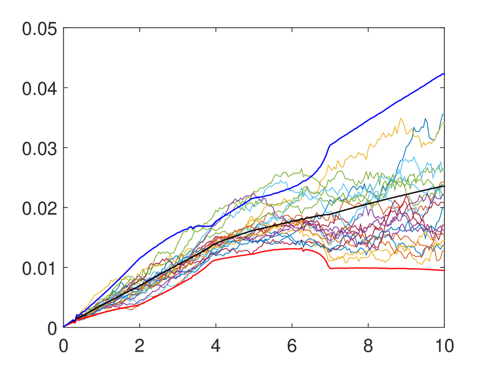
(IF2) Refer to caption Refer to caption

(IF3) Refer to caption Refer to caption

Figure 5.4. 20 sample paths of the short rate (top panels) and the price process of a basis swap (bottom panels) for each interpolating function along with the mean (black line) and 97.5% and 2.5% percentiles computed over 105superscript10510^{5} realizations.

(IF1) vs. (IF2) Refer to caption

(IF1) vs. (IF3) Refer to caption

(IF2) vs. (IF3) Refer to caption

Figure 5.5. Absolute difference between the basis swap price processes for different interpolating functions.
Refer to captionRefer to captionRefer to captionRefer to captionRefer to caption

(IF1) vs. (IF2) Refer to caption Refer to caption Refer to caption Refer to caption Refer to caption

(IF1) vs. (IF3) Refer to caption Refer to caption Refer to caption Refer to caption Refer to caption

(IF2) vs. (IF3) Refer to caption Refer to caption Refer to caption Refer to caption Refer to caption

Figure 5.6. 20 sample paths of the TVA process for the basis swap, together with the mean and percentiles, for the 5 different CSA specifications (left panels, top to bottom), and the difference between the TVA processes for the different interpolating functions (left to right).

5.4. Discussion

The outcome of the numerical experiments is summarized in Figures 5.4 until 5.6. Starting with the top panel in Figure 5.4, we observe that there are significant structural differences in the dynamics of the short rate due to the different interpolating functions; this is mostly visible when looking at the averages and the percentile lines. The bottom panel in the same figure displays the price process of the 3M-6M basis swap for the different interpolating functions. As the differences are not as clearly visible as before, we have plotted the absolute differences in prices due to the different interpolating functions in Figure 5.5. There we see that notable differences in prices appear when using different interpolating functions (keep in mind, that the notional amount of the swap equals one, thus the deviations in prices are not negligible). As expected, the largest discrepancies between prices stemming from the first vs. second and the first vs. third interpolating functions occur on the curved section of the manifold used to construct (uk)subscript𝑢𝑘(u_{k}) and (vk)subscript𝑣𝑘(v_{k}). On the contrary, the discrepancies between prices from the second vs. third interpolating functions on the curved section of the manifold are zero, since both functions interpolate linearly in that segment.

The next Figure 5.6 depicts the sample path of the TVA process using the first interpolating function (left panels) for the five different CSA specifications (top to bottom), while the other figures show the differences in the TVA due to the different interpolating functions. The differences in the TVA are one order of magnitude smaller than the differences in prices, however the TVA itself is an order of magnitude smaller than the basis swap price. Reflecting the situation for the prices, the largest discrepancies between TVAs using the first and the other two interpolating functions occur around the curved section of the manifold. However, the discrepancies in the TVA in the flat sections of the manifold are more pronounced than the corresponding discrepancies in prices. The reason is that the interpolation affects value adjustments both via the basis swap price and via the short rate used for discounting, and its effect is propagated in different segments through the backward regression. This becomes clear when one looks at the differences between prices and value adjustments stemming from using the second and third interpolating functions; although the difference in prices is flat zero, the difference in value adjustments is far away from zero.

The numerical examples presented above show that the choice of the interpolating function entails significant model risk. The functions we chose are not especially far apart, in terms of their supremum norm, thus the differences above could become even higher. In fact, the coefficients of the short rate can become arbitrarily large due to the interpolating function. Therefore, both the manifolds on which the sequences u𝑢u and v𝑣v lie and the interpolating function have to be selected with caution, as they can fundamentally change the behaviour of the model.

Appendix A Time-integration of Affine processes

The following result is an extension of Theorem 4.10 in Keller-Ressel (2008).

Theorem A.1.

Let θ:[0,T]0d:𝜃0𝑇subscriptsuperscript𝑑absent0\theta\colon[0,T]\rightarrow\mathbb{R}^{d}_{\geqslant 0} be a bounded function and (Xt)t[0,T]subscriptsubscript𝑋𝑡𝑡0𝑇(X_{t})_{t\in[0,T]} be an affine process on 0dsubscriptsuperscript𝑑absent0\mathbb{R}^{d}_{\geqslant 0}, with functional characteristics F𝐹F and R𝑅R. Then (Xt,0tθuXudu)t[0,T]subscriptsubscript𝑋𝑡superscriptsubscript0𝑡subscript𝜃𝑢subscript𝑋𝑢differential-d𝑢𝑡0𝑇\left(X_{t},\int_{0}^{t}\theta_{u}\circ X_{u}\mathrm{d}u\right)_{t\in[0,T]} is a time-inhomogeneous affine process on 0d×0dsubscriptsuperscript𝑑absent0subscriptsuperscript𝑑absent0\mathbb{R}^{d}_{\geqslant 0}\times\mathbb{R}^{d}_{\geqslant 0} with functional characteristics

F~(t,uX,uY)=F(uX)andR~(t,uX,uY)=(R(uX)+θtuY0).formulae-sequence~𝐹𝑡subscript𝑢𝑋subscript𝑢𝑌𝐹subscript𝑢𝑋a𝑛𝑑~𝑅𝑡subscript𝑢𝑋subscript𝑢𝑌𝑅subscript𝑢𝑋subscript𝜃𝑡subscript𝑢𝑌0\widetilde{F}\left(t,u_{X},u_{Y}\right)=F\left(u_{X}\right)\quad{\text{a}nd}\quad\widetilde{R}\left(t,u_{X},u_{Y}\right)=\left(\begin{array}[]{c}R\left(u_{X}\right)+\theta_{t}\circ u_{Y}\\ 0\end{array}\right).

Here \circ denotes the componentwise multiplication between vectors.

Proof.

Let n𝑛n\in\mathbb{N}, k{0,,n}𝑘0𝑛k\in\left\{0,\dots,n\right\}, and define sk=knssubscript𝑠𝑘𝑘𝑛𝑠s_{k}=\frac{k}{n}s and h=sn𝑠𝑛h=\frac{s}{n}, hence s0,,snsubscript𝑠0subscript𝑠𝑛s_{0},\dots,s_{n} is an equidistant partition of [0,s]0𝑠[0,s] with step size hh. Approximating the integral with Riemann sums and using the dominated convergence theorem, we have

𝔼[exp(uX,Xt+s+uY,tt+sθrXrdr)|t]𝔼delimited-[]conditionalsubscript𝑢𝑋subscript𝑋𝑡𝑠subscript𝑢𝑌superscriptsubscript𝑡𝑡𝑠subscript𝜃𝑟subscript𝑋𝑟differential-d𝑟subscript𝑡\displaystyle\mathds{E}\left[\left.\exp\left(\left\langle u_{X},X_{t+s}\right\rangle+\left\langle u_{Y},\int_{t}^{t+s}\theta_{r}\circ X_{r}\mathrm{d}r\right\rangle\right)\right|\mathcal{F}_{t}\right]
=limn𝔼[exp(uX,Xt+s+uY,hk=0nθt+skXt+sk)|t]absentsubscript𝑛𝔼delimited-[]conditionalsubscript𝑢𝑋subscript𝑋𝑡𝑠subscript𝑢𝑌superscriptsubscript𝑘0𝑛subscript𝜃𝑡subscript𝑠𝑘subscript𝑋𝑡subscript𝑠𝑘subscript𝑡\displaystyle\qquad=\lim_{n\rightarrow\infty}\mathds{E}\left[\left.\exp\left(\left\langle u_{X},X_{t+s}\right\rangle+\left\langle u_{Y},h\sum_{k=0}^{n}\theta_{t+s_{k}}\circ X_{t+s_{k}}\right\rangle\right)\right|\mathcal{F}_{t}\right]
=:limnAn.\displaystyle\qquad=:\lim_{n\rightarrow\infty}A_{n}.

Using next the tower law of conditional expectations and the affine property of X𝑋X, Ansubscript𝐴𝑛A_{n} can be written as follows

Ansubscript𝐴𝑛\displaystyle A_{n} =𝔼[𝔼[euX+huYθt+sn,Xt+sn|t+sn1]euY,hk=0n1θt+skXt+sk|t]absent𝔼delimited-[]conditional𝔼delimited-[]conditionalsuperscriptesubscript𝑢𝑋subscript𝑢𝑌subscript𝜃𝑡subscript𝑠𝑛subscript𝑋𝑡subscript𝑠𝑛subscript𝑡subscript𝑠𝑛1superscriptesubscript𝑢𝑌superscriptsubscript𝑘0𝑛1subscript𝜃𝑡subscript𝑠𝑘subscript𝑋𝑡subscript𝑠𝑘subscript𝑡\displaystyle=\mathds{E}\left[\left.\mathds{E}\left[\left.\mathrm{e}^{\left\langle u_{X}+hu_{Y}\circ\theta_{t+s_{n}},X_{t+s_{n}}\right\rangle}\right|\mathcal{F}_{t+s_{n-1}}\right]\mathrm{e}^{\left\langle u_{Y},h\sum_{k=0}^{n-1}\theta_{t+s_{k}}\circ X_{t+s_{k}}\right\rangle}\right|\mathcal{F}_{t}\right]
=𝔼[eϕh(uX+huYθt+sn)+ψh(uX+huYθt+sn),Xt+sn1+uY,hk=0n1θt+skXt+sk|t]absent𝔼delimited-[]conditionalsuperscriptesubscriptitalic-ϕsubscript𝑢𝑋subscript𝑢𝑌subscript𝜃𝑡subscript𝑠𝑛subscript𝜓subscript𝑢𝑋subscript𝑢𝑌subscript𝜃𝑡subscript𝑠𝑛subscript𝑋𝑡subscript𝑠𝑛1subscript𝑢𝑌superscriptsubscript𝑘0𝑛1subscript𝜃𝑡subscript𝑠𝑘subscript𝑋𝑡subscript𝑠𝑘subscript𝑡\displaystyle=\mathds{E}\left[\left.\mathrm{e}^{\phi_{h}\left(u_{X}+hu_{Y}\circ\theta_{t+s_{n}}\right)+\left\langle\psi_{h}\left(u_{X}+hu_{Y}\circ\theta_{t+s_{n}}\right),X_{t+s_{n-1}}\right\rangle+\left\langle u_{Y},h\sum_{k=0}^{n-1}\theta_{t+s_{k}}\circ X_{t+s_{k}}\right\rangle}\right|\mathcal{F}_{t}\right]
=𝔼[𝔼[e(ψh(uX+huYθt+sn)+huYθt+sn1,Xt+sn1)|t+sn2]\displaystyle=\mathds{E}\left[\mathds{E}\left[\left.\mathrm{e}^{\left(\left\langle\psi_{h}\left(u_{X}+hu_{Y}\circ\theta_{t+s_{n}}\right)+hu_{Y}\circ\theta_{t+s_{n-1}},X_{t+s_{n-1}}\right\rangle\right)}\right|\mathcal{F}_{t+s_{n-2}}\right]\right.
×euY,hk=0n2θt+skXt+sk|t]eϕh(uX+huYθt+sn)\displaystyle\qquad\left.\left.\times\ \mathrm{e}^{\left\langle u_{Y},h\sum_{k=0}^{n-2}\theta_{t+s_{k}}\circ X_{t+s_{k}}\right\rangle}\right|\mathcal{F}_{t}\right]\mathrm{e}^{\phi_{h}\left(u_{X}+hu_{Y}\circ\theta_{t+s_{n}}\right)}
=𝔼[eψh(ψh(uX+huYθt+sn)+huYθt+sn1),Xt+sn2+uY,hk=0n2θt+skXt+sk|t]absent𝔼delimited-[]conditionalsuperscriptesubscript𝜓subscript𝜓subscript𝑢𝑋subscript𝑢𝑌subscript𝜃𝑡subscript𝑠𝑛subscript𝑢𝑌subscript𝜃𝑡subscript𝑠𝑛1subscript𝑋𝑡subscript𝑠𝑛2subscript𝑢𝑌superscriptsubscript𝑘0𝑛2subscript𝜃𝑡subscript𝑠𝑘subscript𝑋𝑡subscript𝑠𝑘subscript𝑡\displaystyle=\mathds{E}\left[\left.\mathrm{e}^{\left\langle\psi_{h}\left(\psi_{h}\left(u_{X}+hu_{Y}\circ\theta_{t+s_{n}}\right)+hu_{Y}\circ\theta_{t+s_{n-1}}\right),X_{t+s_{n-2}}\right\rangle+\left\langle u_{Y},h\sum_{k=0}^{n-2}\theta_{t+s_{k}}\circ X_{t+s_{k}}\right\rangle}\right|\mathcal{F}_{t}\right]
×eϕh(uX+huYθt+sn)+ϕh(ψh(uX+huYθt+sn)+huYθt+sn1).absentsuperscriptesubscriptitalic-ϕsubscript𝑢𝑋subscript𝑢𝑌subscript𝜃𝑡subscript𝑠𝑛subscriptitalic-ϕsubscript𝜓subscript𝑢𝑋subscript𝑢𝑌subscript𝜃𝑡subscript𝑠𝑛subscript𝑢𝑌subscript𝜃𝑡subscript𝑠𝑛1\displaystyle\qquad\times\ \mathrm{e}^{\phi_{h}\left(u_{X}+hu_{Y}\circ\theta_{t+s_{n}}\right)+\phi_{h}\left(\psi_{h}\left(u_{X}+hu_{Y}\circ\theta_{t+s_{n}}\right)+hu_{Y}\circ\theta_{t+s_{n-1}}\right)}.

Iterating this procedure, we arrive at

An=exp(pn(uX,uY)+qn(uX,uY),Xt),subscript𝐴𝑛subscript𝑝𝑛subscript𝑢𝑋subscript𝑢𝑌subscript𝑞𝑛subscript𝑢𝑋subscript𝑢𝑌subscript𝑋𝑡A_{n}=\exp\Big{(}p_{n}\left(u_{X},u_{Y}\right)+\left\langle q_{n}\left(u_{X},u_{Y}\right),X_{t}\right\rangle\Big{)},

with p0(uX,uY)=0subscript𝑝0subscript𝑢𝑋subscript𝑢𝑌0p_{0}\left(u_{X},u_{Y}\right)=0, q0(uX,uY)=uX+huYθt+ssubscript𝑞0subscript𝑢𝑋subscript𝑢𝑌subscript𝑢𝑋subscript𝑢𝑌subscript𝜃𝑡𝑠q_{0}\left(u_{X},u_{Y}\right)=u_{X}+hu_{Y}\circ\theta_{t+s} and

pk+1(uX,uY)subscript𝑝𝑘1subscript𝑢𝑋subscript𝑢𝑌\displaystyle p_{k+1}\left(u_{X},u_{Y}\right) =pk(uX,uY)+ϕh(qk(uX,uY))absentsubscript𝑝𝑘subscript𝑢𝑋subscript𝑢𝑌subscriptitalic-ϕsubscript𝑞𝑘subscript𝑢𝑋subscript𝑢𝑌\displaystyle=p_{k}\left(u_{X},u_{Y}\right)+\phi_{h}\left(q_{k}\left(u_{X},u_{Y}\right)\right)
qk+1(uX,uY)subscript𝑞𝑘1subscript𝑢𝑋subscript𝑢𝑌\displaystyle q_{k+1}\left(u_{X},u_{Y}\right) =ψh(qk(uX,uY))+huYθt+sn(k+1).absentsubscript𝜓subscript𝑞𝑘subscript𝑢𝑋subscript𝑢𝑌subscript𝑢𝑌subscript𝜃𝑡subscript𝑠𝑛𝑘1\displaystyle=\psi_{h}\left(q_{k}\left(u_{X},u_{Y}\right)\right)+hu_{Y}\circ\theta_{t+s_{n-(k+1)}}.

Using the generalized Riccati equation (2.3), we can expand ϕitalic-ϕ\phi and ψ𝜓\psi linearly around the origin. Thus we get

pk+1(uX,uY)subscript𝑝𝑘1subscript𝑢𝑋subscript𝑢𝑌\displaystyle p_{k+1}\left(u_{X},u_{Y}\right) =pk(uX,uY)+hF(qk(uX,uY))+o(h),absentsubscript𝑝𝑘subscript𝑢𝑋subscript𝑢𝑌𝐹subscript𝑞𝑘subscript𝑢𝑋subscript𝑢𝑌𝑜\displaystyle=p_{k}\left(u_{X},u_{Y}\right)+hF\left(q_{k}\left(u_{X},u_{Y}\right)\right)+o\left(h\right),
qk+1(uX,uY)subscript𝑞𝑘1subscript𝑢𝑋subscript𝑢𝑌\displaystyle q_{k+1}\left(u_{X},u_{Y}\right) =qk(uX,uY)+h(R(qk(uX,uY))+uYθsn(k+1))+o(h).absentsubscript𝑞𝑘subscript𝑢𝑋subscript𝑢𝑌𝑅subscript𝑞𝑘subscript𝑢𝑋subscript𝑢𝑌subscript𝑢𝑌subscript𝜃subscript𝑠𝑛𝑘1𝑜\displaystyle=q_{k}\left(u_{X},u_{Y}\right)+h\left(R\left(q_{k}\left(u_{X},u_{Y}\right)\right)+u_{Y}\circ\theta_{s_{n-(k+1)}}\right)+o\left(h\right).

As θ𝜃\theta is nonnegative and bounded, the second part of the proof of Theorem 4.10 in Keller-Ressel (2008) remains the same. Hence, the recursive scheme above is an Euler-type approximation, starting from the terminal time, to the ODE

sp(s,t,uX,uY)𝑠𝑝𝑠𝑡subscript𝑢𝑋subscript𝑢𝑌\displaystyle\frac{\partial}{\partial s}p\left(s,t,u_{X},u_{Y}\right) =F(q(s,t,uX,uY)),absent𝐹𝑞𝑠𝑡subscript𝑢𝑋subscript𝑢𝑌\displaystyle=F\left(q\left(s,t,u_{X},u_{Y}\right)\right),
sq(s,t,uX,uY)𝑠𝑞𝑠𝑡subscript𝑢𝑋subscript𝑢𝑌\displaystyle\frac{\partial}{\partial s}q\left(s,t,u_{X},u_{Y}\right) =R(q(s,t,uX,uY))+uYθsabsent𝑅𝑞𝑠𝑡subscript𝑢𝑋subscript𝑢𝑌subscript𝑢𝑌subscript𝜃𝑠\displaystyle=R\left(q\left(s,t,u_{X},u_{Y}\right)\right)+u_{Y}\circ\theta_{s}

with initial conditions p(r,r,uX,uY)=0𝑝𝑟𝑟subscript𝑢𝑋subscript𝑢𝑌0p\left(r,r,u_{X},u_{Y}\right)=0 and q(r,r,uX,uY)=uX𝑞𝑟𝑟subscript𝑢𝑋subscript𝑢𝑌subscript𝑢𝑋q\left(r,r,u_{X},u_{Y}\right)=u_{X}, for all r0𝑟0r\geq 0. ∎

References

  • Beveridge and Joshi (2012) C. Beveridge and M. Joshi. Interpolation schemes in the displaced-diffusion LIBOR market model. SIAM J. Financial Math., 3:593–604, 2012.
  • Bichuch et al. (2016) M. Bichuch, A. Capponi, and S. Sturm. Arbitrage-free XVA. Math. Finance (forthcoming), 2016.
  • Björk (2009) T. Björk. Arbitrage Theory in Continuous Time. Oxford University Press, 3rd edition, 2009.
  • Brigo et al. (2013) D. Brigo, M. Morini, and A. Pallavicini. Counterparty Credit Risk, Collateral and Funding: with Pricing Cases for all Asset Classes. Wiley, 2013.
  • Crépey (2015a) S. Crépey. Bilateral Counterparty risk under funding constraints — Part I: Pricing. Math. Finance, 25:1–22, 2015a.
  • Crépey (2015b) S. Crépey. Bilateral Counterparty risk under funding constraints — Part II: CVA. Math. Finance, 25:23–50, 2015b.
  • Crépey and Bielecki (2014) S. Crépey and T. R. Bielecki. Counterparty Risk and Funding: A Tale of two Puzzles. Chapman & Hall/CRC Financial Mathematics Series. CRC Press, 2014. With an introductory dialogue by Damiano Brigo.
  • Crépey et al. (2012) S. Crépey, Z. Grbac, and H.-N. Nguyen. A multiple-curve HJM model of interbank risk. Math. Financ. Econ., 6:155–190, 2012.
  • Crépey et al. (2013) S. Crépey, R. Gerboud, Z. Grbac, and N. Ngor. Counterparty risk and funding: The four wings of the TVA. Int. J. Theor. Appl. Finance, 16(1350006), 2013.
  • Cuchiero et al. (2016) C. Cuchiero, C. Fontana, and A. Gnoatto. Affine multiple yield curve models. Preprint, arXiv:1603.00527, 2016.
  • Duffie et al. (2003) D. Duffie, D. Filipović, and W. Schachermayer. Affine processes and applications in finance. Ann. Appl. Probab., 13:984–1053, 2003.
  • Filipović (2005) D. Filipović. Time-inhomogeneous affine processes. Stochastic Process. Appl., 115:639–659, 2005.
  • Glau et al. (2016) K. Glau, Z. Grbac, and A. Papapantoleon. A unified view of LIBOR models. In J. Kallsen and A. Papapantoleon, editors, Advanced Modelling in Mathematical Finance – In Honour of Ernst Eberlein, pages 423–452. Springer, 2016.
  • Grbac and Runggaldier (2015) Z. Grbac and W. J. Runggaldier. Interest Rate Modeling: Post-Crisis Challenges and Approaches. Springer, 2015.
  • Grbac et al. (2015) Z. Grbac, A. Papapantoleon, J. Schoenmakers, and D. Skovmand. Affine LIBOR models with multiple curves: theory, examples and calibration. SIAM J. Financial Math., 6:984–1025, 2015.
  • Jacod and Shiryaev (2003) J. Jacod and A. N. Shiryaev. Limit Theorems for Stochastic Processes. Springer, 2nd edition, 2003.
  • Keller-Ressel (2008) M. Keller-Ressel. Affine Processes: Theory and Applications to Finance. PhD thesis, TU Vienna, 2008.
  • Keller-Ressel (2009) M. Keller-Ressel. Affine LIBOR models with continuous tenor. Unpublished manuscript, 2009.
  • Keller-Ressel et al. (2013) M. Keller-Ressel, A. Papapantoleon, and J. Teichmann. The affine LIBOR models. Math. Finance, 23:627–658, 2013.
  • Mercurio (2009) F. Mercurio. Interest rates and the credit crunch: New formulas and market models. Preprint, SSRN/1332205, 2009.
  • Mercurio (2010) F. Mercurio. A LIBOR market model with a stochastic basis. Risk, pages 84–89, December 2010.
  • Musiela and Rutkowski (1997) M. Musiela and M. Rutkowski. Continuous-time term structure models: forward measure approach. Finance Stoch., 1:261–291, 1997.
  • Musiela and Rutkowski (2005) M. Musiela and M. Rutkowski. Martingale Methods in Financial Modelling. Springer, 2nd edition, 2005.
  • Papapantoleon (2010) A. Papapantoleon. Old and new approaches to LIBOR modeling. Stat. Neerlandica, 64:257–275, 2010.