Airborne contaminant source estimation using a finite-volume forward solver coupled with a Bayesian inversion approach

Abstract

We consider the problem of estimating emissions of particulate matter from point sources. Dispersion of the particulates is modelled by the 3D advection-diffusion equation with delta-distribution source terms, as well as height-dependent advection speed and diffusion coefficients. We construct a finite volume scheme to solve this equation and apply our algorithm to an actual industrial scenario involving emissions of airborne particulates from a zinc smelter using actual wind measurements. We also address various practical considerations such as choosing appropriate methods for regularizing noisy wind data and quantifying sensitivity of the model to parameter uncertainty. Afterwards, we use the algorithm within a Bayesian framework for estimating emission rates of zinc from multiple sources over the industrial site. We compare our finite volume solver with a Gaussian plume solver within the Bayesian framework and demonstrate that the finite volume solver results in tighter uncertainty bounds on the estimated emission rates.

url]http://www.math.sfu.ca/ stockie

1 Introduction

Dispersion of pollutants in the atmosphere and their subsequent impacts on the environment are major sources of concern for many large industrial operations and the government agencies that monitor their emissions. For this reason, assessing environmental risks is a normal aspect of ongoing industrial activities, particularly when any new or expanded operation is being considered. Atmospheric dispersion models play a crucial role in impact assessment studies where they are routinely studied with the aid of computer simulations. An overview of the different aspects of atmospheric dispersion modelling can be found in the articles [25, 45] while a self contained and detailed introduction can be found in the monographs [32, 43].

In general, numerical methods for atmospheric dispersion modelling can be split into two classes: (1) semi-analytic methods that utilize some approximate analytical solution to the underlying partial differential equations (PDE); and (2) numerical solvers that use finite volume or finite element methods to approximate the underlying PDE with minimal simplifying assumptions. The semi-analytic methods include the class of Gaussian plume solvers. These models have been widely studied in the literature (see [47] and the references therein) and are implemented in industry-standard software such as AERMOD [8] and CALPUFF [42]. The semi-analytic solvers are efficient but they are often based on several simplifying assumptions that may not apply in all emissions scenarios. A few of the common assumptions are that the solution is steady state (even in the presence of time-varying wind) and flow is advection-dominated (so that dispersion in the wind direction can be neglected). In contrast, the direct numerical solvers, such as finite volume or finite element methods, are more flexible and allow for complicated geometry and physical processes but they are often expensive to evaluate (see the monograph [52] and the series of articles [5, 6, 7] for a detailed comparison between different direct solvers). Comparisons between semi-analytic and direct numerical solvers are plentiful in the literature and we refer the reader to the articles [1, 10, 28, 35, 41] for examples of such comparisons.

In this article we focus on short-range dispersion and deposition of heavy particulate matter from an industrial site, where “short” refers to distances of at most a few kilometers. Short-range deposition is of significance in impact assessments for emissions of massive particulate material that has potentially long-term impacts on the environment because the maximum deposition of these particulates occurs close to the sources due to their higher density. We are inspired by an earlier paper of Lushi and Stockie [27], who considered emissions from a lead-zinc smelter located in Trail, British Columbia, Canada. These authors studied the inverse source identification problem, in which their objective was to use a Gaussian plume model to determine the rate of zinc emissions from several point sources given measurements of wind velocity and zinc deposition. In contrast with this earlier work, we propose in this paper a finite volume solver that directly handles a time-varying wind field and also takes into account vertical variations of both wind velocity and eddy diffusion coefficients, thereby avoiding some of the brute simplifications inherent in Gaussian plume models. Although a finite volume solver can be expensive to evaluate compared with a Gaussian plume approach, we show that by exploiting the linear dependence of the deposition data on the emission rates one can nonetheless significantly reduce the total cost of the model evaluations.

Source inversion in atmospheric dispersion has attracted much attention in recent years [15, 45]. Methodologies for solving the source inversion problem can be split broadly into the two classes of variational and probabilistic methods. In the former approach one formulates the inverse problem as an optimization problem and utilizes convex optimization tools to find an estimate to the emission rates that gives a good match to the measured data. The latter approach obtains a probability distribution on the parameters that describes the emission rates. In this article, we solve the source inversion problem using a Bayesian approach that belongs to the class of probabilistic methods. Recent examples of applications of the Bayesian approach in the literature include the work of Senocak et al. [44] where a Gaussian plume forward model was used within a Bayesian framework in order to estimate the location and rate of emissions of a source. Ristic et al. [36] solve the problem of locating a source using approximate Bayesian computation techniques and compare three different Gaussian plume models to solve the inverse problem. The work of Keats et al. [23] is more closely related to this article, since they used a finite volume solver to construct the forward map within a Bayesian framework in order to infer the location and emission rate for a point source. A similar approach was employed by Hosseini and Stockie [19] to estimate the time-dependent behavior of emissions for a collection of point sources that are not operating at steady state. Here, we use a finite volume solver that was developed in [17] within a hierarchical Bayesian framework in order to infer the rate of emissions of multiple sources in an industrial site. We assume that emission rates are constant in time and that the locations of the sources are known. The main challenge in our setting derives from the fact that data is only available in the form of accumulated measurements of deposition over long times (within dust-fall jars) and so we do not have access to real-time measurement devices. This means that estimating temporal variations in source emissions is not possible. The hierarchical Bayesian framework minimizes the effect of the prior distribution and allows the algorithm to calibrate itself. Furthermore, the Bayesian framework provides a natural way of quantifying the uncertainties in the estimated emission rates and we leverage this ability to perform an uncertainty propagation study that allows us to study the effect of the sources on the surrounding environment. Finally, we compare our finite volume solver with the Gaussian plume solver of [27] in the context of the Bayesian inversion algorithm. We demonstrate that the finite volume solver results in smaller uncertainties in the estimated emission rates, which is strong evidence of the superiority of the finite volume approach.

The remainder of this article is organized as follows. We begin in Section 2 by presenting a general model for dispersion and settling of particulate matter in the atmosphere, based on an advection-diffusion PDE. We also provide details regarding the functional forms for variable coefficients that are commonly applied in atmospheric science applications. In Section 3, we develop a finite volume scheme for solving this variable coefficient advection-diffusion problem in three dimensions. In Section 4, we present an industrial case study involving dispersion of zinc from four major sources, and use our numerical solver to study the impact of these sources on the area surrounding the smelter. We also address various practical aspects of atmospheric dispersion modelling, such as regularizing noisy wind data and studying sensitivity of our model to unknown parameters such as mixing-layer height and atmospheric stability class. In section 5 we introduce the Bayesian framework for solution of the source inversion problem and obtain and estimate of the emission rates for four sources on the industrial site in Trail, BC, Canada. Finally, we compare the solution of the inverse problem when our finite volume solver is used to obtain the forward map to the setting where a Gaussian plume solver is used to solve the forward problem.

2 Mathematical model for pollutant dispersion and deposition

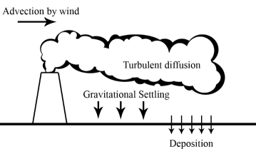
We begin by developing a mathematical model based on the advection-diffusion equation, which is a linear partial differential equation (PDE) capable of capturing a wide range of phenomena involving transport of particulate material in the atmosphere. In particular, we are concerned with the release of contaminants from elevated point sources (such as stacks or chimneys), advective transport by a time-varying wind field, diffusion due to turbulent mixing, vertical settling of particles due to gravitational effects, and deposition of particulate material at the ground surface. This scenario is depicted in Figure 1. The effects of deposition are especially important since a common and inexpensive technique for monitoring pollutant emissions is by means of dust-fall jars, which measure a monthly accumulated deposition of particulate matter at fixed locations. We also focus attention on short-range particulate transport over distances on the order of a few kilometres.

Figure 1: Diagram depicting the primary mechanisms of advection, diffusion, settling and deposition for particulate material released from a single stack-like point source.

Before proceeding any further, we first provide a list of several main simplifying assumptions:

1. Variations in ground topography are negligible, so that the ground surface can be taken to be a horizontal plane.

2. The wind velocity is assumed horizontal and spatially-uniform within each horizontal plane. This follows naturally from assumption (i) and is reasonable since we are only interested in short-range transport. We allow horizontal velocity components to change with altitude owing to effects of the atmospheric boundary layer. These are necessary assumptions because wind measurements are only available at a few locations, so that there is insufficient data to permit reconstruction of a detailed wind field.

3. A (small) constant vertical component is included in the advection velocity for each particulate, which accounts for the settling velocity of solid particles.

4. Pollutant sources take the form of stacks or vents on top of buildings that are small in comparison with the transport length scales, so that all can be approximated as point sources.

5. The terrain is relatively uniform so that there is no need to differentiate between areas having different deposition characteristics owing to ground coverage by buildings, trees, pavement, etc. As a result, variations in the roughness length that is needed to describe the ground surface can be ignored.

6. We consider only dry deposition and ignore any effects of wash-out due to wet deposition that might occur during rainfall events.

In the following sections, we present the equations, boundary conditions and coefficient functions without detailed justification since the model is standard in the atmospheric science literature and can be found in references such as [32, 43].

2.1 Atmospheric dispersion as a 3D advection–diffusion problem

Based on the above assumptions, we can describe the transport of an airborne pollutant in three spatial dimensions using the advection–diffusion equation

$$\frac{\partial c(\mathbf{x},t)}{\partial t}+\nabla\cdot\left(\mathbf{u}(\mathbf{x},t)c+\mathbf{S}(\mathbf{x},t)\nabla c\right)=q(\mathbf{x},t)\qquad\text{on }\Omega\times(0,T),$$ (1)

where $c(\mathbf{x},t)\>[\mbox{$\mathrm{kg/m^{3}}$}]$ denotes the mass concentration (or density) of a certain pollutant at time $t\>[\mbox{$\mathrm{s}$}]$ and the spatial domain is the half-space $\Omega:=\{\mathbf{x}=(x,y,z):z\geq 0\}$, where $z$ denotes height above the ground surface. The wind velocity field is denoted $\mathbf{u}(\mathbf{x},t)=\left(u_{x}(\mathbf{x},t),u_{y}(\mathbf{x},t),u_{z}(\mathbf{x},t)\right)\>[\mbox{$\mathrm{m/s}$}]$ and $\mathbf{S}(\mathbf{x},t):=\textbf{diag}\left(s_{x}(\mathbf{x},t),s_{y}(\mathbf{x},t),s_{z}(\mathbf{x},t)\right)[\mbox{$\mathrm{m^{2}/s}$}]$ represents a diagonal turbulent eddy diffusion matrix having non-negative entries, $s_{\{x,y,z\}}(\mathbf{x},t)\geq 0$. Because the size of any individual pollutant source is assumed much smaller than the typical length scale for transport, we can approximate the source term as a superposition of point sources, $q(\mathbf{x},t):=\sum_{i=1}^{N_{q}}q_{i}(t)\,\delta(\mathbf{x}-\mathbf{x}_{q,i})$, where $N_{q}$ is the number of sources, $\mathbf{x}_{q,i}$ is the location of the $i^{th}$ source (after correcting for vertical plume rise effects), and $\delta(\mathbf{x})$ is the 3D Dirac delta distribution.

We assume that the particle concentration is negligible at distances far enough from the sources, so that we can impose the far-field boundary condition

$$c(\mathbf{x},t)\to 0\quad\text{as }\left|\mathbf{x}\right|\to\infty.$$ (2)

At the ground surface ($z=0$) we impose a mixed (Robin) boundary condition to capture the deposition flux of particulate material following [43, Ch. 19] as

$$\left.\left(u_{\text{set}}c+s_{z}\frac{\partial c}{\partial z}\right)\right|_{z=0}=\left.u_{\text{dep}}c\right|_{z=0},$$ (3)

where $u_{\text{dep}}>0$ is the particle deposition velocity (an experimentally-determined constant) and $u_{\text{set}}$ is the settling velocity given for spherical particles by Stokes’ law as

$$u_{\text{set}}=\frac{\rho gd^{2}}{18\mu}.$$ (4)

Here, $\rho\>[\mbox{$\mathrm{kg/m^{3}}$}]$ is the particle density, $d\>[\mbox{$\mathrm{m}$}]$ is the particle diameter, $g=9.8\>[\mbox{$\mathrm{m/s^{2}}$}]$ is the gravitational acceleration, and $\mu=1.8\times 10^{-5}\>[\mbox{$\mathrm{kg/m\,s}$}]$ is the viscosity of air. Note that equation (3) assumes the deposition rate (or flux) is proportional to ground-level concentration, and we take this deposition rate equal to the sum of advective and diffusive fluxes so that total mass of pollutant is conserved.

2.2 Wind velocity profile

Recall assumption (ii) that the vertical wind velocity is equal to the constant settling velocity, whereas the horizontal components vary with altitude; that is, $\mathbf{u}(\mathbf{x},t)=(u_{x}(z,t),u_{y}(z,t),u_{\text{set}})$. Next, let $u_{h}(z,t)=\left(u_{x}^{2}(z,t)+u_{y}^{2}(z,t)\right)^{1/2}$ denote the magnitude of the wind velocity in the horizontal plane, and assume the well-known power-law correlation from [32]

$$u_{h}(z,t)=u_{r}(t)\,\left(\frac{z}{z_{r}}\right)^{\gamma},$$ (5)

which approximates the variation of $u_{h}$ with altitude within the atmospheric boundary layer. Here, $u_{r}(t)$ represents the measured wind velocity at a reference height $z_{r}$, and $\gamma$ is a fitting parameter that varies from $0.1$ for a smooth ground surface up to $0.4$ for very rough surfaces in urban areas.

2.3 Eddy diffusion coefficients

The eddy diffusion coefficients $(s_{x},s_{y},s_{z})$ capture the effect of pollutant mixing due to turbulence, and so they only yield an accurate representation if we consider distances much larger than the typical turbulent length scales, which are on the order of tens of meters [33]. These coefficients are typically difficult to measure in practice and so they often experience large errors. We will use a simple model that incorporates the dependence of eddy diffusion parameters on both altitude and wind speed as described in [43, Ch. 18].

2.3.1 Vertical diffusion coefficient (${s_{z}}$)

Following the Monin-Obukhov similarity theory [30], the vertical eddy diffusivity is written

$$s_{z}(z,t)=\frac{\kappa u_{*}(t)z}{\phi(z/L)},$$ (6)

where $\kappa$ is the von Karman constant and can be well-approximated by the value $0.4$. The form of the function

$$\phi(\bar{z})=\begin{cases}(1-15\bar{z})^{1/2},&\text{unstable (classes A, B, C)},\\ 1,&\text{neutral (class D)},\\ 1+4.7\bar{z},&\text{stable (classes E, F)},\end{cases}$$ (7)

is dictated by the Pasquill classification for atmospheric stability, with classes labelled A–F in Table 2 ranging from very unstable to highly stable conditions. The parameter $u_{*}(t)$ is known as the friction velocity and is commonly expressed as a function of the roughness length $z_{0}$ (listed in Table 1 for different types of terrain) and the measured reference velocity $u_{r}$:

$$u_{*}(t)=\frac{\kappa u_{r}(t)}{\ln(h_{r}/z_{0})},$$ (8)

The parameter $L$ is the Monin-Obukhov length [43], which we estimate using an expression from Golder [13] as

$$\frac{1}{L}=a+b\>\log_{10}z_{0}.$$ (9)

Parameters $a$ and $b$ are determined based on the Pasquill stability class and are also listed in Table 2. By combining equations (6)–(9), we have a method for computing $s_{z}(z,t)$ based on stability class and measured wind velocity.

Surface type	$z_{0}\>(\mbox{$\mathrm{m}$})$
Very smooth (ice, mud)	$10^{-5}$
Snow	$10^{-3}$
Smooth sea	$10^{-3}$
Level desert	$10^{-3}$
Lawn	$10^{-2}$
Uncut grass	$0.05$
Full grown root crops	$0.1$
Tree covered	$1$
Low-density residential	$2$
Central business district	$5$–$10$

Table 1: Surface roughness parameter $z_{0}$ for various terrain types, taken from [29].

Pasquill stability class	$a$	$b$
A (Extremely unstable)	$-0.096$	$0.029$
B (Moderately unstable)	$-0.037$	$0.029$
C (Slightly unstable)	$-0.002$	$0.018$
D (Neutral)	$0$	$0$
E (Slightly stable)	$0.004$	$-0.018$
F (Moderately stable)	$0.035$	$-0.036$

Table 2: Monin-Obukhov length parameters for different stability classes, taken from [43].

Note that the vertical diffusion coefficient vanishes at ground level, which leads to an inconsistency in the deposition boundary condition (3) arising ultimately from a scale mismatch in the vicinity of the ground (recall that the diffusive flux in (3) only makes sense if the typical length scale of interest is much larger than the turbulent length scale). In order to avoid this inconsistency, we regularize $s_{z}$ in a manner similar to what was done for the wind velocity in (5), utilizing the same cutoff height $z_{\text{cut}}$.

2.3.2 Horizontal diffusion coefficient ($s_{x}$ and $s_{y}$)

The horizontal diffusion coefficients are less well-studied than the vertical coefficients, mainly because they are more difficult to measure in practice. A commonly-used expression based on measurements of standard deviations in Gaussian plume models for unstable Pasquill classes [43] is

$$s_{x}(t)=s_{y}(t)\simeq 0.1u_{*}z_{i}^{3/4}(-\kappa L)^{-1/3},$$ (10)

where $z_{i}$ is the mixing layer height (ranging from 100 to 3000 meters depending on topography, stability and time of year) and we have assumed that $s_{x}=s_{y}$ based on symmetry considerations. Note that these horizontal diffusivities are independent of height, in contrast with the vertical diffusivity.

3 Finite volume algorithm

When designing a numerical algorithm to solve the forward model outlined in the previous section, the first issue that needs to be addressed is the impracticality of directly applying the far-field boundary condition (2), since that would require computing on an infinite domain. Instead, we truncate the domain and consider the finite rectangular box $\Omega_{h}:=[0,H_{x}]\times[0,H_{y}]\times[0,H_{z}]\subset\mathbb{R}^{3}$ having dimensions $H_{x}$, $H_{y}$ and $H_{z}$ in the respective coordinate directions. We also consider a finite time interval of length $T$ and denote the space-time domain as $\Omega_{T}:=\Omega_{h}\times(0,T]$. The computational domain $\Omega_{h}$ should be chosen large enough that it contains all sources and wind/dust-fall measurement locations, and so that the distance between any source and the boundary is large enough that concentration and diffusive fluxes along the boundary are negligible. Other than the boundary condition at ground level $z=0$ (which remains unchanged), the far-field condition (2) is replaced by an outflow boundary condition on advection terms and a homogeneous Neumann condition on diffusion terms, both of which are simply special cases of a more general Robin condition.

The linear advection–diffusion problem, along with modified boundary conditions for the truncated domain, can therefore be written in the generic form

$$\begin{cases}\displaystyle\frac{\partial c(\mathbf{x},t)}{\partial t}+\nabla\cdot(\mathbf{f}_{A}(\mathbf{x},t)+\mathbf{f}_{D}(\mathbf{x},t))=q(\mathbf{x},t)&\text{in }\Omega_{T},\\[5.69046pt] \alpha(\mathbf{x})c+\beta(\mathbf{x})\,\nabla c\cdot\mathbf{n}=0&\text{on }\partial\Omega_{h}\times(0,T],\\[5.69046pt] c(\mathbf{x},0)=c_{0}(\mathbf{x})&\text{on }\Omega_{h},\end{cases}$$ (11)

where $c(\mathbf{x},t)$ is the scalar quantity of interest, $\mathbf{f}_{A}$ and $\mathbf{f}_{D}$ are advective and diffusive fluxes, $q(\mathbf{x},t)$ is the source term, and $\mathbf{n}$ is the unit outward normal vector to the boundary $\partial\Omega_{h}$. The advective and diffusive fluxes take the form

$$\mathbf{f}_{A}:=\mathbf{u}(\mathbf{x},t)\,c\quad\text{and}\quad\mathbf{f}_{D}:=-\mathbf{S}(\mathbf{x},t)\,\nabla c,$$ (12)

where $\mathbf{u}(z,t)$ and $\mathbf{S}(\mathbf{x},t)$ are the velocity and diffusivity matrix as before.

We now discuss a constraints on the given functions appearing above. As long as $\mathbf{u}$, $\mathbf{S}$, $\alpha(\mathbf{x})$ and $\beta(\mathbf{x})$ are sufficiently regular (i.e., it is enough for them to be continuous functions) and the matrix $\mathbf{S}$ is positive definite, then we are guaranteed that (11) has a unique solution (see [11, Ch. 9]). In the context of the point source emissions problem, we are interested in singular sources consisting of a finite sum of delta distributions so that $q\in(C^{\infty}_{c}(\Omega_{T}))^{*}$; that is, the source term should be a bounded linear functional on test functions in the solution domain. Finally, the initial concentration is assumed to satisfy $c_{0}\in L^{2}(\Omega_{h})$ in general, although in the atmospheric dispersion context we will typically set $c_{0}=0$.

We now discretize the problem in space by dividing the domain into an equally-spaced grid of $N_{x}$, $N_{y}$ and $N_{z}$ points in the respective coordinate directions. The corresponding grid spacings are $\Delta x=H_{x}/N_{x}$, $\Delta y=H_{y}/N_{y}$ and $\Delta z=H_{z}/N_{z}$, and grid point locations are denoted by $x_{i}=(i-1)\Delta x$ for $i=1,2,\cdots,N_{x}+1$, and similarly for $y_{j}$ and $z_{k}$. The time interval $T$ is divided into $N_{T}$ sub-intervals delimited by points $t_{n}$ for $n=0,1,2,\cdots,N_{T}$, which are not necessarily equally-spaced. In the following four sections, we provide details of our numerical scheme by describing separately the time discretization (using a Godunov type splitting), the spatial discretization for both advection and diffusion terms, and the source term approximation.

3.1 Godunov time splitting

Equation (11) is posed in three spatial dimensions and so can be challenging to solve efficiently, especially if the flow is advection-dominated. We seek an algorithm that approximates advection terms accurately and resolves fine spatial scales, while also allowing the solution to be integrated over long time intervals on the order of weeks to months. The class of splitting schemes satisfies these criteria, and we choose to apply a Godunov-type splitting that treats separately the advection and diffusion terms in each direction, as well as the source term. When applied over a discrete time interval $t\in[t_{n},t_{n+1}]$, the Godunov splitting takes the following form:

$$\frac{\partial c^{(\text{1a})}}{\partial t}+\frac{\partial}{\partial x}\left(u_{x}c^{(\text{1a})}\right)=0, \quad c^{(\text{\text{1a}})}(t_{n})=c(t_{n}),$$ (13a)

$$\frac{\partial c^{(\text{1b})}}{\partial t}+\frac{\partial}{\partial y}\left(u_{y}c^{(\text{1b})}\right)=0, \quad c^{(\text{\text{1b}})}(t_{n})=c^{(\text{1a})}(t_{n+1}),$$ (13b)

$$\frac{\partial c^{(\text{1})}}{\partial t}+\frac{\partial}{\partial z}\left(u_{z}c^{(\text{1})}\right)=0, \quad c^{(\text{\text{1}})}(t_{n})=c^{(\text{1b})}(t_{n+1}),$$ (13c)

$$\frac{\partial c^{(\text{2a})}}{\partial t}-\frac{\partial}{\partial x}\left(s_{x}\frac{\partial c^{(\text{2a})}}{\partial x}\right)=0, \quad c^{(\text{\text{2a}})}(t_{n})=c^{(\text{1})}(t_{n+1}),$$ (13d)

$$\frac{\partial c^{(\text{2b})}}{\partial t}-\frac{\partial}{\partial y}\left(s_{y}\frac{\partial c^{(\text{2b})}}{\partial y}\right)=0, \quad c^{(\text{\text{2b}})}(t_{n})=c^{(\text{2b})}(t_{n+1}),$$ (13e)

$$\frac{\partial c^{(\text{2})}}{\partial t}-\frac{\partial}{\partial z}\left(s_{z}\frac{\partial c^{(\text{2})}}{\partial z}\right)=0, \quad c^{(\text{\text{2}})}(t_{n})=c^{(\text{2b})}(t_{n+1}),$$ (13f)

$$\frac{\partial c^{(\text{3})}}{\partial t}-q=0, \quad c^{(\text{\text{3}})}(t_{n})=c^{(\text{2})}(t_{n+1}),$$ (13g)

$$c(t_{n+1})=c^{(\text{\text{3}})}(t_{n+1}).$$ (13h)

Thus, we need to solve a sequence of advection and diffusion problems in each coordinate direction between times $t_{n}$ and $t_{n+1}$, and then in a final step take into account the contribution of the source term. This Godunov splitting is formally first-order accurate in time so that the leading order temporal error of the scheme is $\mathcal{O}(\Delta t)$, where the time step $\Delta t_{n}=t_{n+1}-t_{n}$ [20, 26] and $\Delta t:=\max_{n}(\Delta t_{n})$. The main advantage of this approach is that each of (13a)–(13f) is a one-dimensional problem that can be solved efficiently to obtain a solution of the full 3D problem.

Before moving onto details of the spatial discretization, we need to describe the effect of splitting on the boundary conditions (11), which relies on recognizing that the Robin boundary condition is simply a combination of advective and diffusive fluxes. Recalling that the advection terms in (13) are dealt with using outflow boundary conditions, we can impose the following flux condition on each boundary face:

$${\mathbf{f}}_{A}(\mathbf{x},t)=\min\{0,-(\mathbf{u}(\mathbf{x},t)\cdot\mathbf{n})~{}c\}\quad\text{for }\mathbf{x}\in\partial\Omega_{h}.$$ (14)

After that, we can impose the following modified Robin condition on the diffusion equations

$$\alpha(\mathbf{x})c+\beta(\mathbf{x})\,\nabla c\cdot\mathbf{n}=\max\{0,(\mathbf{u}(\mathbf{x},t)\cdot\mathbf{n})~{}c\}\quad\text{for }\mathbf{x}\in\partial\Omega_{h}.$$ (15)

Formally adding (14) and (15) yields the original boundary condition in (11), and this splitting introduces an additional $\mathcal{O}(\Delta t)$ error due to the boundary condition approximation [20].

3.2 Discretizing advection in 1D

Because each of the split advection equations (13a)–(13c) involves derivatives in only one coordinate direction, we demonstrate here how to discretize a generic 1D advection equation in $x$, after which the corresponding discretizations in $y$ and $z$ are straightforward. The subject of numerical methods for conservation laws (for which 1D advection is the simplest example) is well-studied, and we refer the reader to [26] for an extensive treatment. We make use of a simple upwinding approach and implement the advection algorithm using the Clawpack software package [9].

Consider the following pure advection problem in 1D

$$\begin{cases}\displaystyle\frac{\partial c}{\partial t}+\frac{\partial}{\partial x}\left(cu(x,t)\right)=0,\\[5.69046pt] f_{A}(0,t)=\min\{0,u(0,t)\,c\},\\[5.69046pt] f_{A}(H_{x},t)=\min\{0,-u(H_{x},t)\,c\},\\[5.69046pt] c(x,0)=c_{0}(x),\end{cases}$$ (16)

for $x\in[0,H_{x}]$ and $t\in(0,T]$, where $f_{A}$ denotes a scalar advective flux analogous to the vector flux appearing in (11). Let $\mathcal{C}_{i}=[x_{i},x_{i+1}]$ represent a finite volume grid cell and take $C_{i,n}$ to be a piecewise constant approximation to $c(x,t_{n})$ at all points $x\in\mathcal{C}_{i}$. Then, define $U_{i,n}:=u(x_{i},t_{n})$ which can be interpreted as a piecewise constant approximation of the advection velocity.

Using forward Euler time-stepping and upwinding for the discrete fluxes in each cell yields the explicit scheme

$$C_{i,n+1}=C_{i,n}+\frac{\Delta t_{n}}{\Delta x}\bigg{[}(\max\{0,U_{i,n}\}-\min\{0,-U_{i,n}\})C_{i-1,n}\\ +(\min\{0,-U_{i,n}\}-\min\{0,-U_{i+1,n}\}-\max\{0,U_{i,n}\}+\max\{0,U_{i+1,n}\})C_{i,n}\\ +(\min\{0,-U_{i+1,n}\}-\max\{0,-U_{i+1,n}\})C_{i+1,n}\;\bigg{]},$$ (17)

which holds at interior cells $i=2,3,\cdots,N-1$ and has an error of $\mathcal{O}(\Delta t,\Delta x)$. Boundary conditions for advection are imposed using ghost cells (see [26, Ch. 7]). Note that our choice of boundary fluxes in (16) only allows the quantity $c$ to leave the domain but prevents any influx. This boundary condition can be easily implemented by setting $C_{0,n}=C_{N+1,n}=0$, which define values of the solution at ghost cells lying at points located one grid spacing outside the domain.

This explicit advection scheme introduces a stability restriction in each step of the form $\max_{i}({\left|U_{i,n}\right|})\frac{\Delta t_{n}}{\Delta x}<\nu<1$, called the CFL condition. Because velocity changes with time, we need to choose $\Delta t_{n}$ adaptively to ensure that the Courant number $\nu$ is less than 1 in all grid cells at each time step. Ideally, we would like to maintain $\nu$ as close to 1 as possible in order to minimize artificial diffusion in the computed solution (see [26] for an in-depth discussion); however, when the velocity field varies significantly in $x$, then this may not be feasible and some smearing is unavoidable.

3.3 Discretizing diffusion in 1D

We use a similar approach to discretize the diffusion equation in 1D, for which we take the generic problem

$$\begin{cases}\displaystyle\frac{\partial c}{\partial t}-\frac{\partial}{\partial x}\left(s(x,t)\frac{\partial c}{\partial x}\right)=0&\text{for }(x,t)\in(0,H_{x})\times(0,T],\\[5.69046pt] \displaystyle\alpha(t)c+\beta(t)\frac{\partial c}{\partial x}=0&\text{at }x=0,\\[5.69046pt] \displaystyle\tilde{\alpha}(t)c+\tilde{\beta}(t)\frac{\partial c}{\partial x}=0&\text{at }x=H_{x},\\[5.69046pt] c(x,0)=c_{0}(x).\end{cases}$$ (18)

On interior cells away from the boundary, we can discretize this equation as

$$C_{i,n+1}=C_{i,n}-\frac{\Delta t_{n}}{\Delta x^{2}}\left[S_{i+1,n+1}(C_{i+1,n+1}-C_{i,n+1})-S_{i,n+1}(C_{i,n+1}-C_{i-1,n+1})\right],$$ (19)

where $S_{i,n}:=s(x_{i},t_{n})$. Here we also define ghost cells $\mathcal{C}_{0}$ and $\mathcal{C}_{N+1}$ to approximate the boundary conditions from (18) as follows:

$$\begin{cases}\displaystyle\alpha(t_{n+1})\frac{C_{0,n+1}+C_{1,n+1}}{2}&+\;\beta(t_{n+1})\displaystyle\frac{C_{1,n+1}-C_{0,n+1}}{\Delta x}=0,\\[5.69046pt] \displaystyle\tilde{\alpha}(t_{n+1})\frac{C_{N,n+1}+C_{N+1,n+1}}{2}&+\;\displaystyle\tilde{\beta}(t_{n+1})\frac{C_{N+1,n+1}-C_{N,n+1}}{\Delta x}=0,\end{cases}$$ (20)

where $C_{0,n+1}=C_{N,n+1}=0$ in order to approximate the outflow boundary conditions. Because this method is implicit in time, it is also unconditionally stable. Therefore, when solved in conjunction with the explicit advection equations, the same time step $\Delta t_{n}$ can be used as long as the appropriate CFL conditions are satisfied for the advection equations.

3.4 Approximating point sources

The final element required to construct the 3D advection–diffusion solver is a discretization of (13g) to incorporate the effect of singular source terms. Using a finite volume approach we obtain the following semi-discrete scheme on cell ${\mathcal{C}_{ijk}}$

$$C^{(3)}_{ijk,n+1}=C^{(2)}_{ijk,n}+\Delta t_{n}\int_{\mathcal{C}_{ijk}}q(\mathbf{x},t_{n})\,d\mathbf{x},$$ (21)

after which all that is needed is to select an appropriate quadrature scheme to evaluate the integral over each cell. Recall that the source terms of interest in our pollutant dispersion application consist of a sum of $N_{q}$ delta distributions

$$q(\mathbf{x},t)=\sum_{i=1}^{N_{q}}q_{i}(t)\,\delta(\mathbf{x}-\mathbf{x}_{s,i}),$$ (22)

with source strengths $q_{i}(t)$ and fixed locations $\mathbf{x}_{s,i}$. Because each source term is singular at $\mathbf{x}=\mathbf{x}_{s,i}$, we need to choose an appropriate regularization of the delta distribution.

Smooth regularizations of the delta distribution have been studied extensively for a wide variety of PDEs and quadrature schemes [18, 48, 49, 50]. Well-known theoretical results are available which show that the spatial order of the solution approximation away from such a singular source is connected to the number of moment conditions that a regularized delta satisfies [18, 49, 50]. We choose a particularly simple piecewise constant approximation

$$\delta_{h}(\mathbf{x})=\begin{cases}\displaystyle\frac{1}{\Delta x\Delta y\Delta z}&\text{if }\mathbf{x}\in[-\Delta x/2,\Delta x/2]\times[-\Delta y/2,\Delta y/2]\times[-\Delta z/2,\Delta z/2],\\[5.69046pt] 0&\text{otherwise},\end{cases}$$ (23)

which satisfies the first moment condition and is therefore known to yield approximations that converge pointwise with second-order spatial accuracy outside the support of the regularized source term. A distinct advantage of this choice of piecewise constant delta regularization is that the integrals in (21) can be performed exactly. Recalling that the discretization of advection terms is first-order accurate in space, it is clearly the error from the discretization of derivative terms that dominates the solution error and not that from the source terms.

3.5 Approximating total deposition

The scheme outlined above yields approximate values of pollutant concentration $c(\mathbf{x},t)$; however, when dealing with particulate deposition we are often concerned with the total amount of particulate material that accumulates over some time interval $(0,T]$ at certain specified locations on the ground (corresponding to the dust-fall jar collectors). The total particulate measured at ground location $(x,y,0)$ can be expressed in the integral form

$$w(x,y,T):=\int_{0}^{T}u_{\text{dep}}\,c(x,y,0,t)\,dt.$$ (24)

Employing a one-sided quadrature in time, we can write the following approximate formula for accumulating deposition $w$ between one time step and the next at location $(x_{i},y_{j},0)$

$$w_{ij,n+1}=w_{ij,n}+\frac{u_{\text{dep}}}{2}(t_{n+1}-t_{n})\left(C_{ij1,n}+C_{ij0,n}\right),$$ (25)

with $w_{ij,0}=0$. Here we used the value of the solution in the ghost cells $\mathcal{C}_{ij0}$ to improve the estimate of concentration at the boundary. This expression follows from our discretization of the Robin boundary conditions in (20).

3.6 Numerical convergence study

So far we have discussed the details of our finite volume algorithm for solution of advection-diffusion PDEs with variable coefficients. We implement this algorithm in Fortran by coupling the diffusion solver of Section 3.3 with the Clawpack 4.3 software package that implements the advection algorithm described in Section 3.2. Implementation of the source term as well as computation of total depositions are also done using Clawpack.

In order to verify the convergence rate of our algorithm, we solve (11) on the cube $\Omega_{h}=\{0\leq x,z\leq 10,\;-5\leq y\leq 5\}$ up to time $T=8.0$. We assume that both the advection velocity and diffusion tensor are height-dependent and have the form $\mathbf{u}(x,y,z)=((z/10)^{0.3},0,0)$ and $\mathbf{S}(x,y,z)=\textbf{diag}(0.25,0.25,s_{z}(z))$, where

$$s_{z}(z)=\frac{z\sqrt{1-15}}{40\sqrt{1-15z/10}}.$$ (26)

To investigate the effect of the point source singularities on the solution accuracy we consider two cases:

1. A smooth source $q_{\text{smooth}}(\mathbf{x},t)=\frac{1}{8}[1+\cos(\pi(x-3))]\cdot[1+\cos(\pi y)]\cdot[1+\cos(\pi(z-3))]$ having support on the smaller cube $\{2\leq x,z\leq 4,\;-1\leq y\leq 1\}$ contained in $\Omega_{h}$.

2. An approximate point source $q_{\text{point}}=\delta_{h}(\mathbf{x}-(3,0,3))$ with $\delta_{h}$ defined as in (23). Note that this source regularization depends on the mesh spacing so that the source term approximation changes as the grid is refined.

We now present the results of a convergence study that investigates the effect on the solution of regularizing the source term. The expected first-order spatial convergence of our algorithm relies on an implicit regularity assumption on the source term which is violated in the case of the point source regularization in case (ii). We aim to show first that for simulations using $q_{\text{smooth}}$, the method is uniformly first-order accurate owing to the regularity of the source term. The simulations are then repeated with $q_{\text{point}}$, which show that first-order convergence is lost over the entire domain, but that the expected order of accuracy can be recovered if we omit from the error estimate any points contained within a suitably small neighbourhood of the source.

To this end, we apply our algorithm on a sequence of uniform grids having $N$ points in each coordinate direction with $N=16,32,64,128$ and 256, and specify the time step size within Clawpack by imposing a maximum Courant number of $\nu=0.9$. To estimate the error in the computed solutions we use the discrete $\ell^{p}$ norms defined by

$$\|\mathbf{v}\|_{\ell^{p}}:=\left(\frac{1}{N}\sum_{i=1}^{N}|v_{i}|^{p}\right)^{1/p}$$ (27)

with $p=1,2$, and $\mathbf{v}$ being any vector with entries $v_{i}$, $i=1,2,\dots,N$. Let $C_{N}$ denote the concentration solution on a grid of size $N$, and define the logarithm of the ratio of differences between successive solutions as

$$E_{p}(N)=\log_{2}\left(\frac{\|C_{N}-C_{2N}\|_{\ell^{p}}}{\|C_{2N}-C_{4N}\|_{\ell^{p}}}\right).$$ (28)

As $N\to\infty$, we expect that $E_{p}(N)$ should approach the value 1 which is the order of spatial convergence for the algorithm. Table 3 lists the computed values of $E_{p}(64)$ for both $q_{\text{smooth}}$ and $q_{\text{point}}$, where we clearly see that the smooth source exhibits first-order accuracy. For the point source when all grid cells in the domain are included, our scheme is only convergences in the case of the $\ell^{1}$-norm, and a rate significantly less than the expected value of 1. However, when the rate is estimated only at points separated from the source, then the convergence rates improve significantly even though they have not yet achieved the expected asymptotic value. These results are consistent with the discussion of delta source approximations in Section 3.4.

	$E_{p}(64)$
Source type	$p=1$	$p=2$
$q_{\text{smooth}}$ (entire domain)	1.0268	1.0481
$q_{\text{point}}$ (entire domain)	0.5365	$-$0.5236
$q_{\text{point}}$ (away from source)	0.6227	0.5560

Table 3: Estimated convergence rates for smooth and singular source terms in the discrete $\ell^{1}$ and $\ell^{2}$ norms.

4 Industrial case study

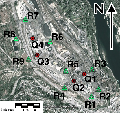
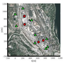
We are now prepared to apply the numerical solver to study an industrial problem concerning the dispersion of zinc from a lead-zinc smelter in Trail, British Columbia, Canada operated by Teck Resources Ltd. An aerial photograph of the industrial site is presented in Figure 2, which indicates the locations of four distinct sources of zinc (Q1–Q4) and nine dust-fall jars (or “receptors”) that take ground-level deposition measurements (R1–R9). A similar emissions scenario at the same industrial site was already considered by Lushi and Stockie [27], who instead employed a Gaussian plume approximation of the particulate transport equation rather than our finite volume approximation. They also solved the inverse source identification problem using a least-squares minimization approach.

Here, we will use our finite volume algorithm to solve the forward emissions problem, and describe the advantages of this approach over the Gaussian plume approximation. We will then use our algorithm to construct the mapping from the source emission rate to the deposition measurements, incorporating this mapping within a Bayesian inversion framework that estimates the emission rates given monthly particulate accumulations within the dust-fall jars. Finally, we study the impact of the estimated emission rates on the area surrounding the industrial site. This approach for solving the inverse problem is closely-related to that in [19], where the source inversion problem for emissions of lead particulates was studied within a Bayesian framework, but instead using a Gaussian plume approximation for the forward solver.

The locations and emission rates for the four sources are listed in Table 4, where we have assumed that emissions are constant in time since the lead-zinc smelter mostly operates at steady state. These emissions are rough engineering estimates provided by the Company, and one of the purposes of this study is to exploit the dust-fall data in order to obtain more accurate approximations of the four emission rates. The pollutant of primary interest in this study is zinc, which manifests mostly in the form of zinc sulphate $\text{ZnSO}_{4}$, for which values of physical parameters are provided in Table 5.

Figure 2: Aerial photo of the smelter site in Trail, British Columbia, Canada. Red dots indicate the main sources of airborne zinc particulates and green triangles are the measurement (dust-fall jar) locations.

Symbol	Emission rate $q_{i}~{}[\mbox{$\mathrm{ton/yr}$}]$	$x$-coordinate ($\mathrm{m}$)	$y$-coordinate ($\mathrm{m}$)	height ($\mathrm{m}$)
Q1	35	748	224.4	15
Q2	80	625.5	176.6	35
Q3	5	255	646	15
Q4	5	251.6	867	15

Table 4: Location and engineering estimates of emission rate for each zinc source.

Parameter	Symbol	Units	Value for $\text{ZnSO}_{4}$
Density	$\rho$	$\mathrm{kg\>m^{-3}}$	$3540$
Molar mass	$M$	$\mathrm{kg\>mol^{-3}}$	$0.161$
Diameter	$d$	$\mathrm{m}$	$5.0\times 10^{-6}$
Deposition velocity	$u_{\text{dep}}$	$\mathrm{m\>s^{-1}}$	$0.005$
Settling velocity	$u_{\text{set}}$	$\mathrm{m\>s^{-1}}$	$0.0027$

Table 5: Values of physical parameters for $\text{ZnSO}_{4}$ particulates, taken from [27].

4.1 Wind data

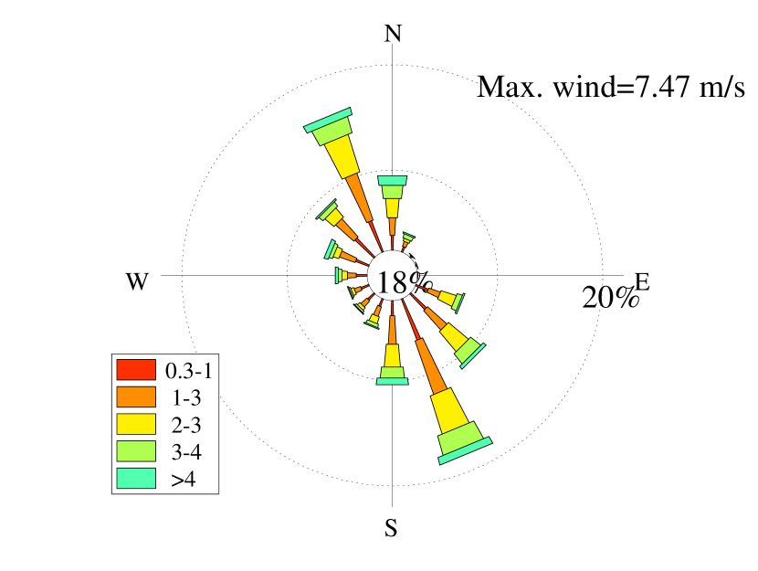
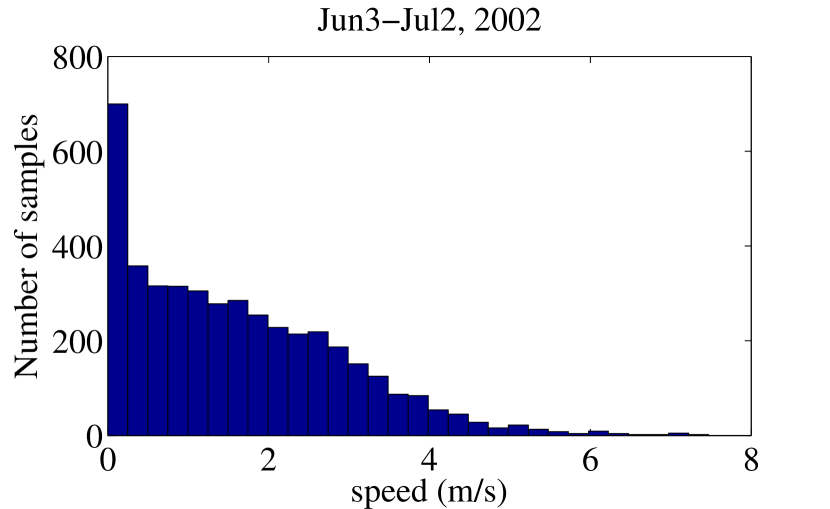
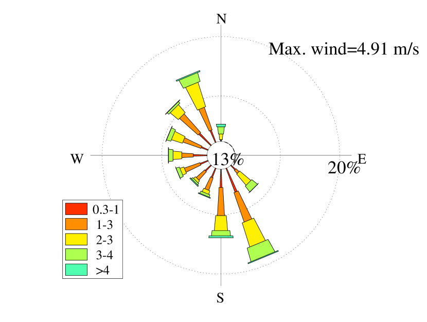
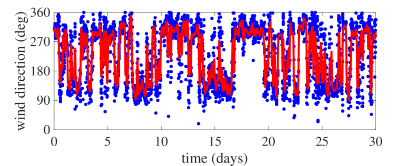
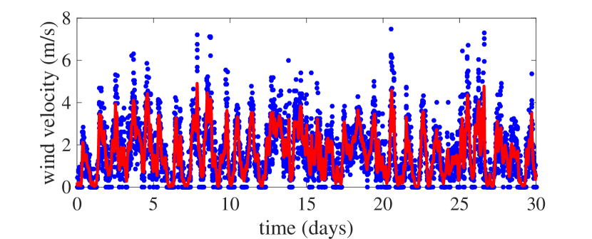
An essential input to our model is the reference wind speed $u_{r}(t)$, which affects both the advection velocity (5) and eddy diffusion coefficients (8). Measurements of horizontal wind speed and direction are provided at 10-minute time intervals from a single meteorological post that is located adjacent to the smelter site (just off the lower right corner of the aerial photo, to the south-east). A wind-rose diagram and histogram of the raw wind measurements are presented in Figure 3 for the period June 3–July 2, 2002. The raw wind data suffers from significant levels of noise (see Figure 4, right) and so it cannot be input directly to our numerical solver, recalling that both $\mathbf{u}(\mathbf{x},t)$ and $\mathbf{S}(\mathbf{x},t)$ must be sufficiently smooth for (11) to have a unique solution. In order to overcome this problem we pre-process the raw wind data by applying a regularization procedure that fits a Gaussian process separately to wind velocity and direction. The details of this fitting step are outside of the scope of this article and so we refer the interested reader instead to the monographs [4, 51] that provide an introduction to the use of Gaussian processes in regression. We employ a Gaussian kernel and ten-fold cross validation, and the resulting regularized velocity components are compared with the raw data in Figure 4. The regularized wind data is clearly smoother in the sense that the direction and velocity experience more gradual variations in time, while the extreme values are also suppressed. This results in a noticeably different wind-rose plot for the regularized data (compare Figures 3 and 4). On the other hand, the regularization process retains the essential patterns such as the dominant northwest and southeast winds, as well as periods of low-to-moderate speed.

Figure 3: Wind-rose plot (left) and wind speed histogram (right) for the raw wind data measured over the period of June 3–July 2, 2002. The wind-rose plots clearly identify a prevailing wind direction during this period.

Figure 4: The regularized wind data displayed as a wind-rose diagram (left) and direction/velocity components (right). In the component plots, blue dots represent the measured wind data and the red line denotes the regularized data.

4.2 Parameter sensitivity analysis

The model in Section 2 contains several input parameters that are difficult to measure accurately. In practice, one typically makes a compromise by approximating certain parameter values using a combination of estimated values from other papers in the literature and/or employing some type of parameter-fitting based on prior knowledge of certain solution variables (such as deposition measurements in the present case). Table 6 summarizes the parameters in this case study for which there is a significant degree of uncertainty, all of which are associated with either the reference velocity or eddy diffusion coefficients. For each of these parameters, we provide a “best guess” along with a “most likely range”. These ranges are informed by both expert knowledge from the Company’s environmental engineering team as well as data from other similar studies in the atmospheric dispersion literature.

Many of these parameters are strongly affected by weather or atmospheric stability class. For the time period of interest (June 3–July 2, 2002) the weather was mostly sunny with minimal rainfall, suggesting that an atmospheric stability class of either unstable or neutral type is most appropriate. Therefore, throughout the rest of this article we will take the stability class to be A. Furthermore, the terrain on the smelter site is a mix of trees, grass, paved areas and buildings, which when combined with the information in Tables 1 and 2 gives suggested ranges for $z_{0}$ and $L$. Values for the velocity exponent $\gamma$ and mixing height $z_{i}$ are selected following the guidelines in [43] for a general class of atmospheric dispersion problems. Finally, we use a range for cut-off length $z_{\text{cut}}$ that is chosen consistent with the average height of the various zinc sources.

Clearly, the lack of accurate site-specific values for these parameters leads to some uncertainty in our simulated results. Therefore, we aim in this section to investigate the sensitivity of the model output to this parameter uncertainty. Sensitivity analysis is a well-developed subject in the areas of applied mathematics, statistics, engineering and applied sciences [14, 39, 46], and some well-known techniques for studying sensitivity of computer models include adjoint methods and brute-force derivative estimation methods. However these approaches focus on local sensitivity and so are not as useful for investigating the effect of varying a parameter over a wide range of values, such as we do here. Instead, we employ a statistical approach that allows quantifying global sensitivity of the model to selected parameters. For this purpose, we employ first-order Sobol indices and total effect indices of the parameters for given functions of the model output. We provide a brief description of these sensitivity measures next and refer the interested reader to [39, Ch. 8] for a detailed discussion.

Consider a set of $p$ normalized parameters $\boldsymbol{\theta}:=(\theta_{1},\theta_{2},\cdots,\theta_{p})$ defined over a unit hypercube $\Theta^{p}\in[0,1]^{p}$, and let $\eta(\boldsymbol{\theta}):\Theta^{p}\to\mathbb{R}$ be some function of interest. In the context of this case study, we have $p=5$ parameters and we are especially interested in scalar-valued functions of the form $\eta:=\mathcal{J}:\Theta^{p}\to\mathbb{R}$. For simplicity, we suppose that the function has zero mean, $\int_{\Theta^{p}}\eta(\boldsymbol{\theta})\,d\boldsymbol{\theta}=0$, from which it follows that the first-order Sobol index $S_{i}$ for parameter $\theta_{i}$ (known as the main effect) is given by

$$S_{i}(\eta):=\frac{\int_{0}^{1}\eta_{i}^{2}(\theta_{i})\,d\theta_{i}}{\int_{\Theta^{p}}\eta^{2}(\boldsymbol{\theta})\,d\boldsymbol{\theta}}\quad\text{where}\quad\eta_{i}(\theta_{i}):=\int_{0}^{1}\cdots\int_{0}^{1}\eta(\boldsymbol{\theta})\>d\theta_{1}\cdots d\theta_{i-1}d\theta_{i+1}\cdots d\theta_{p}.$$ (29)

In essence, this first-order Sobol index compares the variance of $\eta$ when all parameters except $\theta_{i}$ are integrated out against the entire variance of $\eta$; in other words, $S_{i}$ measures how the variation of $\theta_{i}$ controls the variation of $\eta$. Next, let $\boldsymbol{\theta}_{-i}:=(\theta_{1},\cdots,\theta_{i-1},\theta_{i+1},\cdots,\theta_{p})\in\mathbb{R}^{p-1}$ and define the total effect index $S_{-i}$ of the parameter $\theta_{i}$ as

$$S_{-i}(\eta):=1-\frac{\int_{0}^{1}\cdots\int_{0}^{1}\eta_{-i}^{2}(\boldsymbol{\theta}_{-i})\,d\boldsymbol{\theta}_{-i}}{\int_{\Theta^{p}}\eta^{2}(\boldsymbol{\theta})\,d\boldsymbol{\theta}}\quad\text{where}\quad\eta_{-i}(\boldsymbol{\theta}_{-i}):=\int_{0}^{1}\eta(\boldsymbol{\theta})\>d\theta_{i}.$$ (30)

Intuitively, this total effect index measures the combined effect of the parameter $\theta_{i}$ along with all of its interactions with the other parameters. Taken together, the $S_{i}$ and $S_{-i}$ indices provide a quantitative measure of how each parameter controls the output of the model through the function $\eta$.

Computing Sobol indices typically involves evaluating high-dimensional integrals (in this case, five dimensions). In practice, it is not feasible to apply a quadrature rule directly and we will instead use Monte Carlo sampling. Furthermore, our finite volume code represents a costly integrand evaluation in the context of multi-dimensional integration, and so we also construct a surrogate model for the output and perform the Monte Carlo calculations using the surrogate instead. To this end, suppose that $\{\boldsymbol{\theta}_{k}\}_{k=1}^{K}$ is a collection of points in parameter space, which we refer to as the experimental design. Suppose that the computer code is evaluated at these design points and the outputs are collected as a sequence of real values, $\{\eta(\boldsymbol{\theta}_{k})\}_{k=1}^{K}$. Then a surrogate model $\hat{\eta}(\boldsymbol{\theta}):\Theta^{p}\to\mathbb{R}$ is a function of the parameters that interpolates values of the original function at the design points; that is, $\hat{\eta}(\boldsymbol{\theta}_{k})=\eta(\boldsymbol{\theta}_{k})$ for $k=1,\cdots,K$. If $\hat{\eta}$ is to be a good surrogate, then it should be cheap to evaluate and also provide an accurate approximation of $\eta$ over $\Theta^{p}$. Clearly then, the quality of $\hat{\eta}$ depends on many factors such as the method of interpolation, choice of experimental design, regularity of $\eta$, etc.

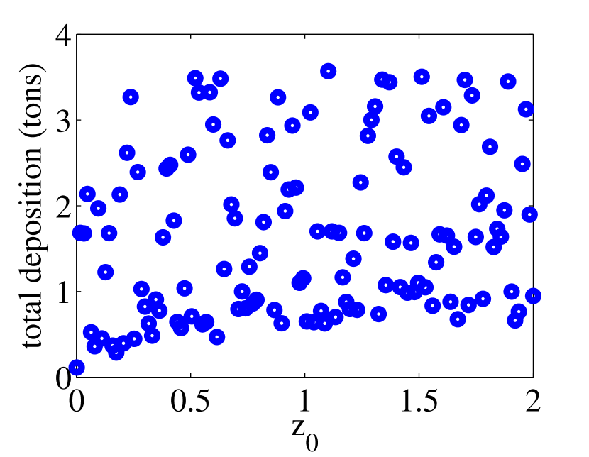
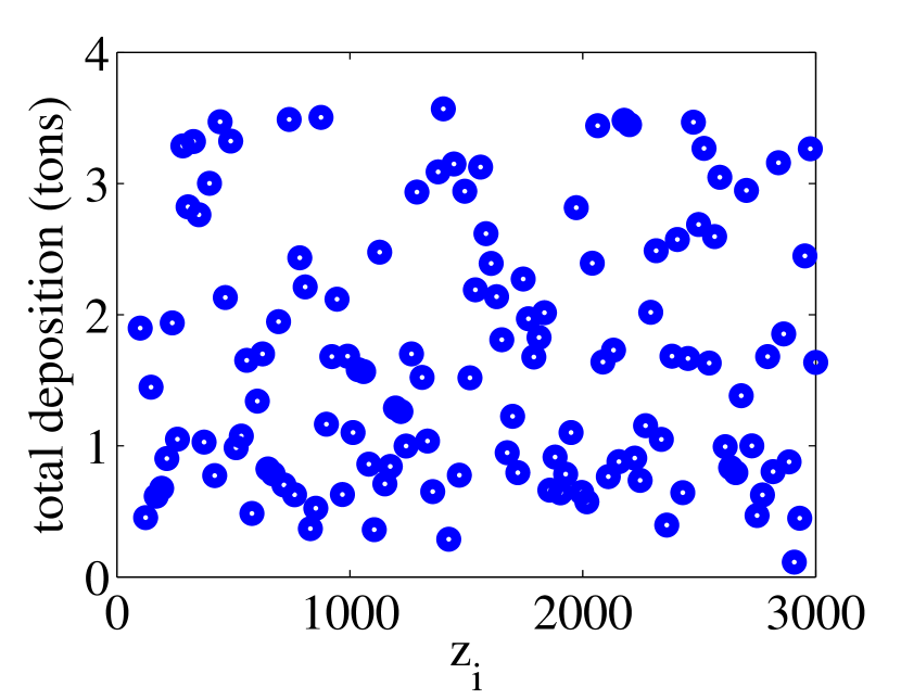
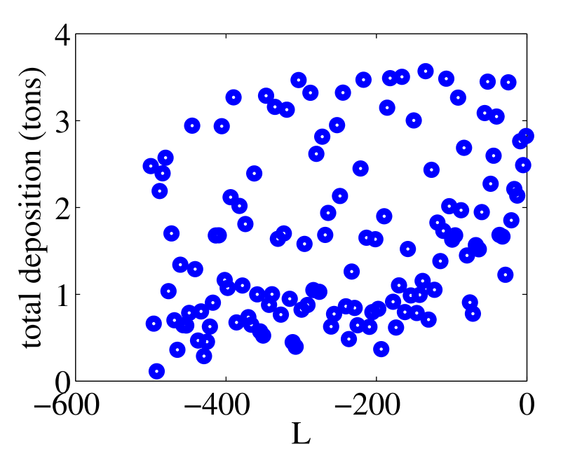
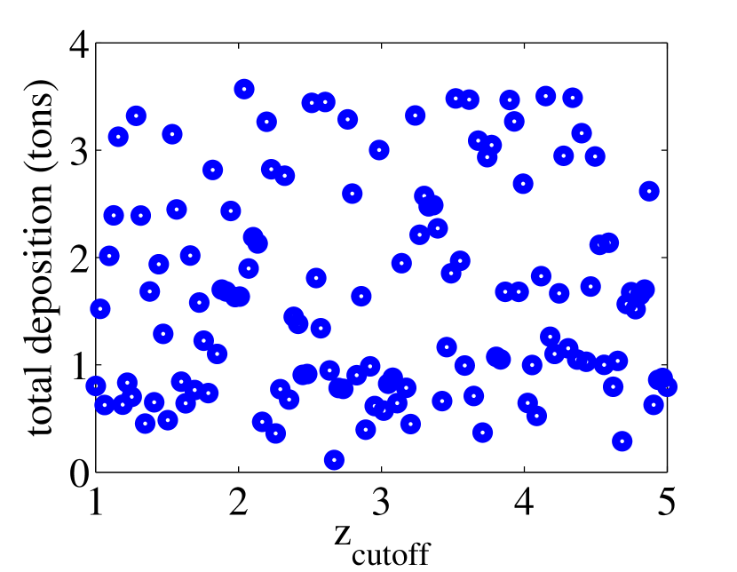
In this case study we consider two quantities of interest that depend on total ground deposition $w$, which in turn depends on parameters through concentration $c$ and the advection-diffusion PDE (1). For now we express these parameter dependencies formally as $\eta=\eta(w;\gamma,z_{0},z_{i},L,z_{\text{cut}})$ and provide the specific form shortly. We employ a space-filling experimental design that consists of 128 points, at each of which the advection-diffusion PDE is solved on a spatial grid of size $50^{3}$ (i.e., $50$ grid points in each coordinate direction) using the regularized wind data from Figure 4. This computation can be done in parallel since the computer experiments are independent. We then use a Gaussian process to construct the surrogate, the details of which can be found in [24, 31] or [40, Section 2.3]. In order to construct the surrogate we compute the quantity of interest $\eta$ from the output of the finite volume solver (the deposition values) and feed this information to the R software package DiceKriging [38], which constructs a Gaussian process surrogate to our finite volume code. Afterwards, we use this surrogate in the R package Sensitivity [34] in order to estimate the Sobol indices.

Parameter	Symbol	Range	Best guess	Equation
Velocity exponent	$\gamma$	$[0.1,0.4]$	$0.3$	(5)
Roughness length ($\mathrm{m}$)	$z_{0}$	$[10^{-3},2]$	$0.1$	(8)
Height of mixing layer ($\mathrm{m}$)	$z_{i}$	$[10^{2},3\times 10^{3}]$	$100$	(10)
Monin-Obukhov length ($\mathrm{m}$)	$L$	$[-500,-1]$	$-8$	(6), (10)
Cut-off length ($\mathrm{m}$)	$z_{\text{cut}}$	$[1,5]$	$2$	–

Table 6: The five problem parameters that are most uncertain, with ranges estimated based on knowledge of smelter site characteristics and typical values used in other atmospheric dispersion studies [43].

In the following two sections, we introduce the two functions $\eta$ of interest and describe how each depends on $w$ and the five parameters. An essential aspect of our study of particulate deposition is to quantify the impact of deposition on the area surrounding the sources. The smelter site depicted in Figure 2 is on the order of 1000 $\mathrm{m}$ across, and immediately outside this area lies several residential zones within a radius of roughly 2000 $\mathrm{m}$. We are therefore interested in differentiating between the particulates being deposited on the smelter site from those occurring within residential areas.

4.2.1 Total deposition in a neighbourhood of the sources

Let $(\bar{x},\bar{y})$ denote the location of the centroid of the industrial site on the ground and consider

$$\eta_{\text{tot}}(w;\gamma,z_{0},z_{i},L,z_{\text{cut}}):=\int_{{\cal B}_{1}}w(x,y,T)\>dx\,dy,$$ (31)

where ${\cal B}_{1}$ represents the ball of radius $R_{1}$ centered at $(\bar{x},\bar{y})$ and $w(x,y,T)$ is the accumulated zinc deposition up to time $T$ from (24). We take $R_{1}=2000~{}\mbox{$\mathrm{m}$}$ and $T=30$ days so that the functional $\eta_{\text{tot}}(w)$ represents total deposition of zinc particulates over a monthly period. The integral is calculated by evaluating $\eta_{\text{tot}}$ at all discrete grid point values lying inside ${\cal B}_{1}$ and then applying the midpoint rule approximation. We note that taking $R_{1}=1000$ instead would not make much difference to the value of $\eta_{\text{tot}}$ since the particulate concentration decreases so rapidly with distance away from the sources.

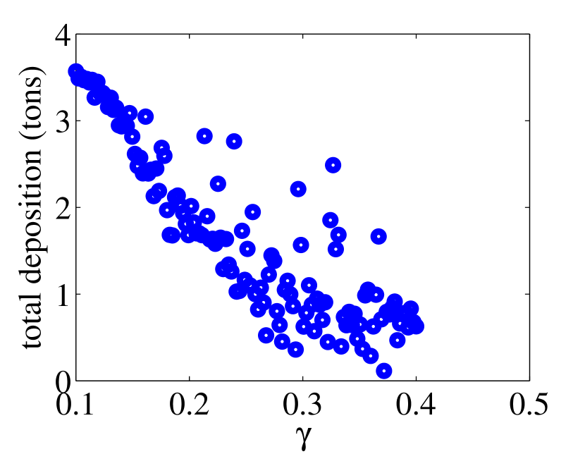
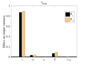
Figure 5 shows the results of our computer experiments with 128 choices of parameters applied to the total deposition functional $\eta_{\text{tot}}$. Note the strong influence of $\gamma$ on the model outputs, particularly in comparison with the other parameters where the influence is much weaker. This dominant influence of $\gamma$ is further supported by the Sobol indices $S_{i}$ and $S_{-i}$ depicted in Figure 7a.

4.2.2 Maximum off-site deposition

The second quantity of interest is the maximum concentration of particulate material deposited outside of the main smelter site, which is of more interest from the point of view of community environmental impact assessment. Even though particulates deposited in close proximity to sources are higher than in residential areas located further away, the only people allowed access to the smelter site are company employees who have the benefit of protective equipment to help deal with the potentially higher concentrations of pollutants. In contrast, inhabitants of nearby areas located in the surrounding community typically do not have such protection, and even though the pollutant concentrations are typically orders of magnitude lower, their potential long-term impacts could still be significant. Therefore, an important aspect of monitoring and protecting communities located adjacent to an industrial operation such as a smelter is to determine whether or not particulate deposition levels off-site ever reach some critical level, which motivates the following functional

$$\eta_{\max}(w;\gamma,z_{0},z_{i},L,z_{\text{cut}}):=\max_{(x,y)\in\bar{\cal B}_{2}}w(x,y,T),$$ (32)

where $\bar{\cal B}_{2}=\mathbb{R}^{2}\setminus{\cal B}_{2}$ represents the area outside the ball ${\cal B}_{2}$ of radius $R_{2}$ where we take $R_{2}=1000\;\mbox{$\mathrm{m}$}$. This functional is easily evaluated by computing the maximum over all grid point values lying outside ${\cal B}_{2}$.

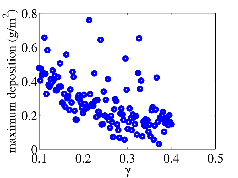
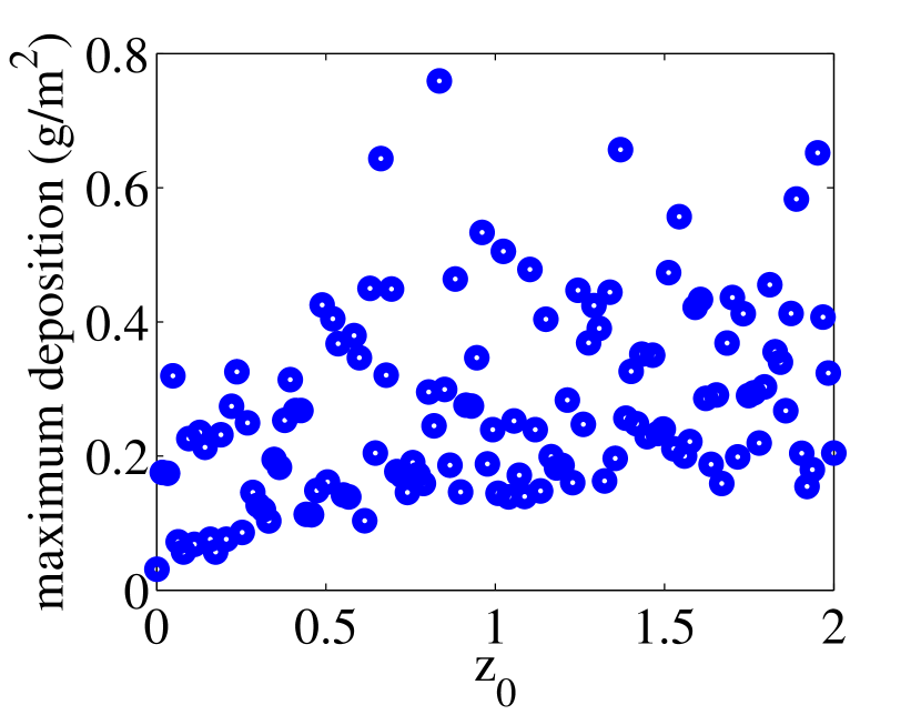
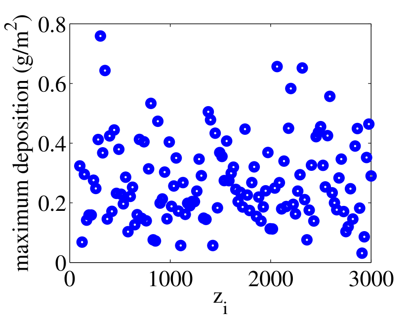
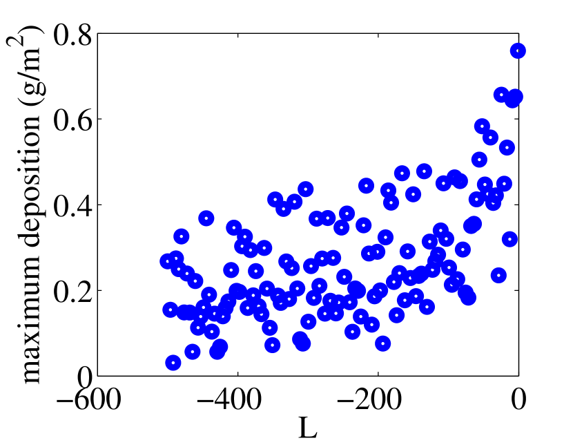
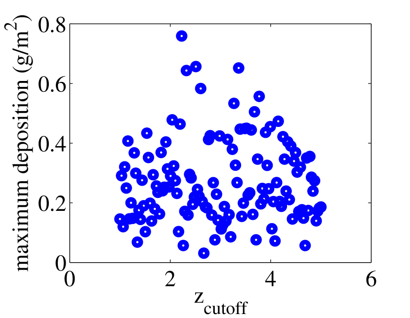
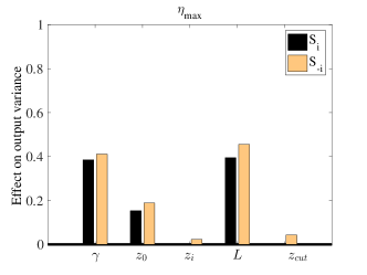
Figure 6 depicts results of numerical experiments based on $\eta_{\max}$, which show that maximum deposition exhibits sensitivity to both the velocity exponent $\gamma$ and Monin-Obukhov length $L$. This result is qualitatively different from the total deposition case, and the differences are particularly apparent from the bar plots of Sobol indices in Figure 7b. Indeed, the Sobol index values indicate that maximum off-site deposition is also sensitive to a third parameter, $z_{0}$. This feature can also be recognized from the slight clustering of points in the $z_{0}$ scatter plot in Figure 6, although the Sobol indices are a more reliable indicator.

Figure 5: Results of 128 computer experiments showing the dependence of total deposition $\eta_{\text{tot}}$ in the vicinity of the smelter on the five key parameters.

Figure 6: Results of 128 computer experiments, showing the dependence of maximum off-site deposition $\eta_{\text{max}}$ on the five key parameters.

a)	b)

Figure 7: Results of the sensitivity analysis depicted in terms of Sobol indices for total deposition in the vicinity of the smelter (left) and maximum deposition away from the site (right). The velocity profile exponent $\gamma$ has a dominant effect on total deposition whereas the maximum off-site deposition is affected significantly by $z_{0}$ and $L$ as well as $\gamma$. For either choice of deposition functional, the remaining parameters $z_{i}$ and $z_{\text{cut}}$ are barely active.

5 Source inversion

We now use the forward solver developed in the previous section to address the problem of determining the emission rates at point sources Q1–Q4 based on the zinc deposited in dust-fall jars R1–R9 (as depicted in Figure 2). The emission rates listed in Table 4 are estimates provided by the Company, based upon engineering calculations and knowledge of the specific chemical and metallurgical processes taking place in each of the four sources at the smelter. Our aim is to improve upon these estimates by solving the source inversion problem using our finite volume algorithm as the forward solver. In particular, we will apply a Bayesian approach to solving the inverse problem, for which a detailed introduction to the theory can be found in the monographs [3, 22].

We assume that the emission rate from each source is constant for the duration of the study and take $q_{i}(t)\equiv q_{i}$ in (22). We employ a smaller computational domain $\Omega=\{-200\leq x\leq 1200,\;-200\leq y\leq 1200,\;0\leq z\leq 300\}$, which is discretized on a $50^{3}$ uniform grid. The regularized wind data from Figure 4 is employed, and parameters $\gamma$, $z_{0}$, $z_{i}$, $L$ and $z_{\text{cut}}$ are fixed at the “best guess” values determined in Table 6. Based upon these assumptions and the fact that source locations are fixed in space, the mapping from emission rates $q_{i}$ to deposition $w$ is linear. We can therefore define the forward map according to the matrix-vector equation

$$\mathbf{w}=\mathbf{F}\mathbf{q},$$ (33)

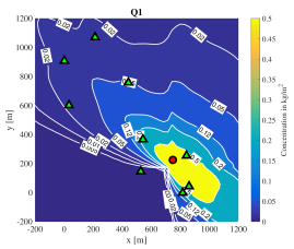
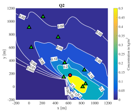
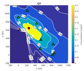
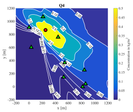
where $\mathbf{F}$ is a $50^{2}\times 4$ matrix, $\mathbf{q}:=(q_{1},q_{2},q_{3},q_{4})^{\text{T}}$ is the emissions vector, and $\mathbf{w}$ is a vector containing the deposition values $w_{ij,N_{T}}$ accumulated over the entire month from (25). The mapping is constructed by solving the forward problem separately for each source based on a unit emission rate. The resulting concentration contour plots are depicted in Figure 8, each of which is concatenated into a single column vector to form the columns of $\mathbf{F}$.

Figure 8: Contour plots of total deposited mass of zinc particulate in the vicinity of the smelter site during June 2–July 3 2002, when each source is given a unit emission rate. These four solutions are concatenated to form the columns of the forward map $\mathbf{F}$ in (33).

Given that the cross-sectional area of each dust-fall jar opening is $A_{\text{jar}}=0.0206\>\mbox{$\mathrm{m^{2}}$}$, which is small relative to the dimensions of a discrete grid cell, we can assume that the jars are point samples of deposition and hence take the $k$-th dust-fall measurement to be

$$d_{k}=w(x_{r_{k}},y_{r_{k}},T)\,A_{\text{jar}},$$ (34)

where $(x_{r_{k}},y_{r_{k}})$ denotes the $k$th sample location. Since the jars aren’t in general aligned with the discrete grid points, the dust-fall deposition estimates are determined from nearby discrete values $\mathbf{w}$ by means of linear interpolation, for which we employ Matlab’s interp2 function. Combining (33) and (34), we obtain the observation map

$$\mathbf{G}:\mathbb{R}^{4}\to\mathbb{R}^{9},\qquad\mathbf{d}=\mathbf{G}\mathbf{q},$$ (35)

where $\mathbf{d}=(d_{1},\cdots,d_{9})^{\text{T}}$ is the vector of dust-fall estimates. The mapping $\mathbf{G}$ is also a linear operator that takes emission rates as input and yields dust-fall measurements as output.

We next describe the source inversion method within the Bayesian framework. We use $\mathbf{d}_{\text{obs}}$ to denote the actual dust-fall jar measurements, and $\mathcal{N}(\mathbf{m},\boldsymbol{\Sigma})$ for a multivariate normal random variable with mean $\mathbf{m}$ and covariance matrix $\boldsymbol{\Sigma}$. Then, denoting by $\pi(\boldsymbol{\xi})$ the Lebesgue density of a multivariate random variable $\boldsymbol{\xi}$, we consider an additive noise model where

$$\mathbf{d}_{\text{obs}}=\mathbf{G}\mathbf{q}+\boldsymbol{\epsilon}\qquad\text{and}\qquad\boldsymbol{\epsilon}\sim\mathcal{N}(0,\sigma^{2}\mathbf{I}_{9\times 9}).$$

Here, $\mathbf{I}_{9\times 9}$ denotes the $9\times 9$ identity matrix and $\sigma>0$ is the standard deviation of the measurement noise, which is computed by assuming a signal-to-noise ratio (SNR) equal to 10 which is chosen based on discussions with experts from the Company. It is then straightforward to verify that the distribution of the data $\mathbf{d}_{\text{obs}}$ conditioned on $\mathbf{q}$ can be written as

$$\pi(\mathbf{d}_{\text{obs}}|\mathbf{q})=\frac{1}{|2\pi\sigma^{2}|^{9/2}}\exp\left(-\frac{1}{2}\|\mathbf{G}\mathbf{q}-\mathbf{d}_{\text{obs}}\|_{2}^{2}\right),$$

which is typically referred to as the likelihood distribution.

The next step in formulating the inverse problem is to construct a prior distribution for the parameter of interest $\mathbf{q}$. Let $\mathbf{q}_{\text{eng}}$ denote the given vector of engineering estimates for emission rates from Table 4. We model prior belief regarding $\mathbf{q}$ via the prior distribution $\pi_{0}$ that is defined through

$$\begin{cases}\pi_{0}(\mathbf{q},\lambda)=\pi_{0}(\mathbf{q}|\lambda)\pi_{0}(\lambda),\\[5.69046pt] \pi_{0}(\mathbf{q}|\lambda)=\mathcal{N}(\mathbf{q},\lambda^{-1}\mathbf{I}_{6\times 6}),\\[5.69046pt] \pi_{0}(\lambda)=\operatorname{Gam}(\alpha_{0},\beta_{0}).\end{cases}$$ (36)

Here, $\operatorname{Gam}(\alpha_{0},\beta_{0})$ is the Gamma distribution with density

$$\operatorname{Gam}(\xi;\alpha_{0},\beta_{0})=\frac{\beta_{0}^{\alpha}}{\Gamma(\alpha_{0})}\xi^{\alpha_{0}-1}\exp\left(-\beta_{0}x\right),$$

where $\Gamma$ denotes the usual gamma function, $\alpha_{0}$ is known as the shape parameter and $\beta_{0}$ is the rate [21]. Put simply, $\pi_{0}$ assumes that prior to observing any measurements the parameter $\mathbf{q}$ is a multivariate normal random variable with an unknown variance $\lambda^{-1}$, where the parameter $\lambda$ is independent of $\mathbf{q}$ and follows a Gamma distribution. Following [16], we take parameters $\alpha_{0}=1$ and $\beta_{0}=10^{-4}$, which implies that $\pi_{0}(\lambda|\mathbf{q})$ has mean $\alpha_{0}/\beta_{0}=10^{4}$ and variance $\alpha_{0}/\beta_{0}^{2}=10^{8}$. This choice of parameters ensures that the prior on $\lambda$ is sufficiently spread out so that it won’t affect the solution to the inverse problem, and hence is essentially “uninformative”.

Applying Bayes’ rule [3, 22] we may now identify the posterior distribution on $\mathbf{q}$ and $\lambda$ as

$$\pi(\mathbf{q},\lambda|y)=\frac{1}{Z}\pi(\mathbf{d}_{\text{obs}}|\mathbf{q})\pi_{0}(\mathbf{q}|\lambda)\pi_{0}(\lambda)\qquad\text{where}\qquad Z=\int\exp\left(-\frac{1}{2}\|\mathbf{G}\mathbf{y}-\mathbf{d}_{\text{obs}}\|_{2}^{2}\right)\pi_{0}(\mathbf{y}|\lambda)\pi_{0}(\lambda)\,d\mathbf{y}\,d\lambda.$$

The quantity $Z$ is simply a normalizing constant that ensures $\pi(\mathbf{q},\lambda|\mathbf{d}_{\text{obs}})$ is a probability density. In practice, we never actually compute $Z$ but instead sample the posterior distribution directly using a Markov Chain Monte Carlo method. Making use of the conjugacy relations between normal and Gamma distributions (see [2] or [12, Sec. 2.4]) we can obtain an analytical expression for the conditional posterior distributions of $\mathbf{q}$ and $\lambda$ as

$$\pi(\mathbf{q}|\lambda,\,\mathbf{d}_{\text{obs}}) =\mathcal{N}\left(\mathbf{q}_{\lambda},\,\mathbf{C}_{\lambda}\right),$$ (37)

$$\pi(\lambda|\mathbf{q},\,\mathbf{d}_{\text{obs}}) =\operatorname{Gam}\left(\alpha_{0}+2,\beta_{0}+\frac{1}{2}\|\mathbf{q}-\mathbf{q}_{\text{eng}}\|_{2}^{2}\right),$$ (38)

where

$$\mathbf{q}_{\lambda} =\mathbf{q}_{\text{eng}}+\lambda^{-1}\mathbf{G}^{\text{T}}(\sigma^{2}\mathbf{I}_{9\times 9}+\lambda^{-1}\mathbf{G}\mathbf{G}^{\text{T}})^{-1}(\mathbf{d}_{\text{obs}}-\mathbf{G}\mathbf{q}_{\text{eng}}),$$ (39)

$$\mathbf{C}_{\lambda} =\lambda^{-1}\mathbf{I}_{4\times 4}-\lambda^{-1}\mathbf{G}^{\text{T}}(\sigma^{2}\mathbf{I}_{9\times 9}+\lambda^{-1}\mathbf{G}\mathbf{G}^{\text{T}})^{-1}\mathbf{G}.$$ (40)

This gives an efficient method for sampling the conditional posterior distributions for both $\mathbf{q}$ and $\mathbf{\lambda}$, and also suggests that a block Gibbs sampler [2, 37] is capable of efficiently sampling the full posterior distribution $\pi(\mathbf{q},\lambda|\mathbf{d}_{\text{obs}})$. Given a large enough sample size $K>0$, our sampling algorithm proceeds as follows:

1. Initialize $\lambda^{(0)}$ and set $k=1$.

2. While $k\leq K$:

   1. Compute $\mathbf{q}^{(k)}\sim\mathcal{N}(\mathbf{q}_{\lambda^{(k-1)}},\mathbf{C}_{\lambda^{(k-1)}})$.

   2. Compute $\lambda^{(k)}\sim\operatorname{Gam}\left(\alpha_{0}+2,\;\beta_{0}+\frac{1}{2}\|\mathbf{q}^{(k)}-\mathbf{q}_{\text{eng}}\|_{2}^{2}\right)$.

   3. Set $k\leftarrow k+1$ and return to step 1.

Note that the finite volume solver enters our framework for solving the inverse problem only through the matrix $\mathbf{F}$ in (33). Once this matrix is in hand, we can construct the observation map $\mathbf{G}$ and sample the posterior distribution using the Gibbs sampler. Here we improve efficiency by constructing the matrix $\mathbf{F}$ in an offline computation using a Fortran implementation of the finite volume algorithm which is coupled with Clawpack (and note further that this computation could also be easily parallelized). After that, we construct $\mathbf{G}$ and solve the actual inverse problem using Matlab.

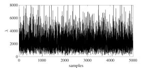
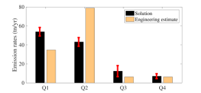
The algorithm just described generates a collection of samples $\{(\mathbf{q}^{(k)},\lambda^{(k)})\}_{k=1}^{K}$ that are distributed according to the posterior distribution $\pi(\mathbf{q},\lambda|\mathbf{d}_{\text{obs}})$. Figure 9 depicts the results of such a computation with sample size $K=5000$, wherein sub-figures a–e depict marginal posterior distributions for $\lambda$ and the emission rates $q_{i}$. Note that the posterior marginals on $q_{i}$ are unimodal and roughly symmetric, which suggests that the mean of posterior $\pi(\mathbf{q}|\mathbf{d}_{\text{obs}})$, denoted $\mathbf{q}_{\text{PM}}$, is a good estimator of the true value of the parameter $\mathbf{q}$. The trace plot of $\lambda$ in Figure 9f exhibits the desirable mixing property of the Gibbs sampler. Finally, Figure 9g compares the engineering estimates $\mathbf{q}_{\text{eng}}$ with the mean of the posterior distribution on the emission rates, denoted by $\mathbf{q}_{\text{PM}}$. The main difference between our solution and the engineering estimates is that the relative size of $Q_{1}$ and $Q_{2}$ is reversed: we clearly identify $Q_{1}$ as the largest source on the site, whereas the Company’s engineering estimates suggest $Q_{2}$ is the largest source. On the other hand, our estimates of $Q_{3}$ and $Q_{4}$ are very close to the engineering estimates. Furthermore, our solution predicts that a total of $116~{}\pm 18~{}\mbox{$\mathrm{ton/yr}$}$ of zinc is emitted from the entire smelter operation, in comparison with the $125~{}\mbox{$\mathrm{ton/yr}$}$ suggested by the engineering estimates, which leaves us confident that our emissions estimates are realistic and are in line with previous studies.

Finally, we study the model predictions of the dust-fall jar data in order to assess the quality of the estimate from the posterior mean. Figure 10 compares the measured data with $\mathbf{q}_{\text{eng}}$ and the predicted data using $\mathbf{q}_{\text{PM}}$. As expected, $\mathbf{q}_{\text{PM}}$ shows a better match with the measurements compared with $\mathbf{q}_{\text{eng}}$, suggesting that the posterior mean yields a significant improvement over the engineering estimates.

a)	b)	c)	d)	e)

f)	g)

Figure 9: Statistical properties of $5000$ samples generated from the posterior distribution $\pi(\mathbf{q},\lambda|\mathbf{d}_{\text{obs}})$ using the Gibbs sampler. (a–e) Marginal posterior distributions of the samples. (f) Trace plot of the Markov chain for $\lambda$ that demonstrates the desirable mixing of the Markov chain. (g) Mean and standard deviation of the vector of emission rates $\mathbf{q}$ in comparison with the engineering estimates $\mathbf{q}_{\text{eng}}$.

Figure 10: Comparison of measured and simulated zinc dust-fall deposition, using wind data from the period June 2–July 3, 2002.

5.1 Uncertainty propagation and impact assessment

With the solution of the inverse problem in hand, we now turn our attention to assessing the impact of the estimated emission rates. To this end, we push the full posterior distribution $\pi(\mathbf{q}|\mathbf{d}_{\text{obs}})$ through the forward map $\mathbf{F}$ (rather than just the posterior mean). Note that the dependence of the posterior on $\lambda$ is suppressed since we are only interested in $\mathbf{q}$. Since this distribution is non-Gaussian we must resort to sampling, which can be expensive. To reduce the computational cost, we will instead approximate the posterior distribution by a Gaussian and obtain an analytical expression for the push-forward of the Gaussian approximation through the forward model. Let $\mathbf{q}_{\text{PM}}$ be the posterior mean of the emission rates as before and let $\mathbf{C}_{\text{post}}$ be the posterior covariance matrix of $\mathbf{q}$, which can be approximated empirically using samples generated by the block Gibbs sampler. We then approximate the posterior distribution $\pi(\mathbf{q}|\mathbf{d}_{\text{obs}})$ using the Gaussian

$$\tilde{\pi}(\mathbf{q}|\mathbf{d}_{\text{obs}})=\mathcal{N}(\mathbf{q}_{\text{PM}},\mathbf{C}_{\text{post}}),$$

with which we obtain an approximation of the probability distribution for total deposition $\mathbf{w}$ as

$$\tilde{\pi}(\mathbf{w})=\mathbf{F}\tilde{\pi}(\mathbf{q}|\mathbf{d}_{\text{obs}})=\mathcal{N}(\mathbf{F}\mathbf{q}_{\text{PM}},\mathbf{F}\mathbf{C}_{\text{post}}\mathbf{F}^{\text{T}}).$$

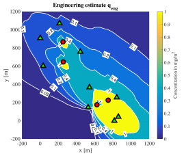
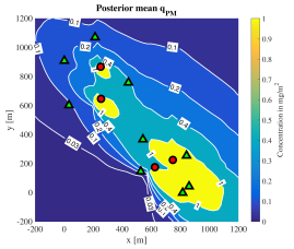
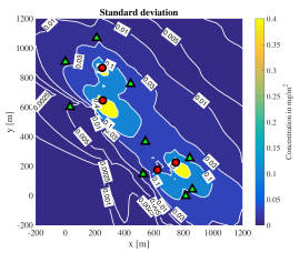
The mean and standard deviation of $\tilde{\pi}(\mathbf{w})$ are displayed in Figure 11 alongside the engineering estimates $\mathbf{q}_{\text{eng}}$ for comparison purposes. As one would expect, the estimate $\mathbf{q}_{\text{PM}}$ results in smaller values of deposition than $\mathbf{q}_{\text{eng}}$; however, the deposition contours have a similar shape. The standard deviation is larger close to the sources and decays rapidly with distance from the sources. Intuitively, this means that the uncertainty in the solution of the inverse problem has a large impact close to the sources but this impact decays as we move away from the sources.

Figure 11: Contours of total deposited pollutant mass in the vicinity of the smelter site, accumulated during the period June 2–July 3, 2002, using the $\mathbf{q}_{\text{eng}}$ and $\mathbf{q}_{\text{PM}}$ estimates (top row) and standard deviation of $\tilde{\pi}(\mathbf{w})$ (bottom left). An aerial map of the smelter site is also included (bottom right).

5.2 Comparison with Gaussian plume solver

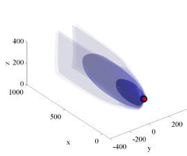
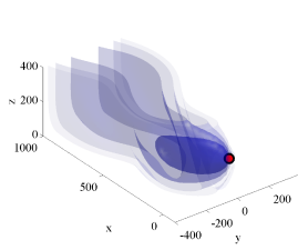
A major advantage of the finite volume solver over the conventional Gaussian plume solution is its ability to capture transient behavior of plumes emitted from point sources and subsequently transported by the wind. In contrast, the Gaussian plume solution typically assumes that both the wind and the advected plume are determined under steady state conditions (the closely-related class of Gaussian puff solutions are capable of handling transient plumes but they have their own set of drawbacks [47]). Figure 12 depicts a typical plume shape arising from a constant unidirectional wind (analogous to the Gaussian plume solution) and compares it with the corresponding plume resulting from a more realistic time-varying wind field (here we imposed a synthetic wind field with a constant speed and sinusoidally-varying direction). The changing wind speed and direction lead to a time-dependent “meandering” motion of the plume in which the plume core with the highest particulate concentrations is deformed significantly relative to the uniform wind case. Contour slices further away from the source location experience a much greater deflection, although they also have less impact on total deposition because the concentration there is much smaller. This example illustrates yet another impact of wind time variations, which is to introduce an additional effective diffusion in the solution, thereby resulting in concentration (and deposition) fields that are much smoother.

Figure 12: Contour slices for a plume arising from a single point source. (left) A constant, uni-directional wind generates the usual Gaussian-shaped plume. (right) A sinusoidally-varying wind direction and speed leads to a meandering plume shape. Both results are computed using the finite volume solver.

We next compare the estimated monthly depositions of zinc using two forward solvers: the finite volume code and the Gaussian plume solution of [19, 27]. The Gaussian plume solver is based on an approximate analytical solution due to Ermak that incorporates a deposition boundary condition consistent with our model (1)–(3). Both solvers use the physical parameter values listed in Table 5, regularized wind data from Figure 4, and diffusion coefficients and wind parameters based on Pasquill stability class A.

Figure 13: Comparison of total deposition contours between the Gaussian plume solver of [27] (left) and our finite volume solver (right). Both solutions are computed using the emission rates obtained from the posterior mean $q_{\text{PM}}$ estimate.

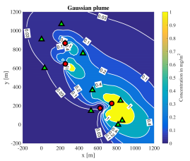
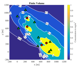
Computed results using the two forward solvers are compared in Figure 13, based on which we observe three main discrepancies. Because the Gaussian plume solution is incapable of capturing plume meander effects due to time-varying winds, the deposition contours computed using this method are more localized and less diffuse. On the other hand, the Gaussian plume solution fails to accurately capture depositions immediately adjacent to the sources because the solution there breaks down in calm winds; consequently, the deposition values near the sources are anomalously low. A third discrepancy arises from the fact that pollutants are not transported as far from the sources with the Gaussian plume solver. It is also important to point out that the discrete time step used in the two simulations is quite different. The Gaussian plume solver computes its quasi-steady solution at time instants separated by a constant interval of 10 minutes, which is justified in [27] based on the size of the domain and wind speed. On the other hand, the finite volume method selects the time step adaptively based on the CFL restriction, which ranges from roughly 1 s (at peak wind speeds) up to a maximum of 40 s (in calm winds). This implies that the finite volume solver is computing with a much smaller time step which improves the wind resolution and corresponding solution accuracy, but comes at the expense of a significant increase in computational cost.

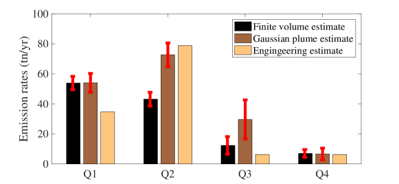
At this point, it is natural to ask how the differences between the two forward models affect the solution to the inverse problem. Recall that our Bayesian framework depends on the finite volume solution only through the observation matrix $\mathbf{G}$ that maps emission rates to dustfall-jar measurements in (35). A direct comparison is then afforded by simply constructing the $\mathbf{G}$ matrix from the Gaussian plume solution and then proceeding to solve the corresponding inverse problem. The result of this computation is presented in Figure 14. Using the Gaussian plume solver we estimate a total of $163.2\pm 31~{}\mbox{$\mathrm{ton/yr}$}$ of zinc is emitted from the entire site, which is larger than the $116\pm 18~{}\mbox{$\mathrm{ton/yr}$}$ estimated using the finite volume solver. Looking more closely at the results, we note that our estimates for $Q_{1}$ and $Q_{4}$ agree quite well between the Gaussian plume and finite volume solvers. However, the estimated values for $Q_{2}$ and $Q_{3}$ using the Gaussian plume solver are significantly larger than those obtained using the finite volume solver. This difference is not surprising if one considers our earlier observation that the two forward models differ significantly in their predictions of near-source depositions (see Figure 13). Given that the uncertainty bounds on the estimates obtained using the finite volume solver are smaller compared to those obtained using the Gaussian plume solver, we conclude that the finite volume solver not only provides more accurate predictions of the measurements but also provides a higher confidence in the solution.

Figure 14: Comparison of estimated emission rates using the finite volume solver and the Gaussian plume solver of [27].

6 Conclusions

In this article we present a model for short-range dispersion and deposition of particulate matter based on a discrete approximation of the advection-diffusion equation. The wind data and eddy diffusion coefficients entering the resulting parabolic partial differential equation allow us to include the effects of atmospheric stability class, surface roughness, and other important parameters. We then presented an efficient finite volume discretization of the PDE that aims to accurately capture the effect of spatially variable coefficients, deposition boundary condition, and concentrated point sources.

The effectiveness of our numerical algorithm was then illustrated using an industrial case study involving the emission of zinc particulates from four point sources located at a zinc smelter. We simulate the results in a statistical framework that allows us to quantify global sensitivity of the model to the five most uncertain parameters. The sensitivity study demonstrates that the velocity exponent $\gamma$ and the Monin-Obukhov length $L$ are the most influential model parameters, suggesting that both require special care to minimize the uncertainty of any numerical simulations based on our model.

We then proceed to solve the inverse problem of estimating the source emission rates from a given set of deposition measurements. We developed a Bayesian framework wherein the forward map was constructed using our finite volume code, and the prior distribution is assumed to follow a normal-Gamma structure. The inverse problem was solved by generating independent samples of the posterior using a Gibbs sampler and then taking the posterior mean as a estimator of the true emission rates. The Bayesian framework provides a natural setting for us to quantify the uncertainty in the solution of the inverse problem. Afterwards, we performed an uncertainty propagation study in order to assess the impact of the estimated emission rates on the area surrounding the industrial site. One of the most useful conclusions of our study was the observation that only four runs of the finite volume code are needed in order to obtain the forward map for the inverse problem. This efficiency gain comes from exploiting the linear dependence of the forward problem on the emission rates, and more than makes up for the smaller time step required in the finite volume scheme relative to other forward solvers like the Gaussian plume.

Finally, we presented a comparison between our finite volume solver and a Gaussian plume solver. The Gaussian plume solver ignores certain physical processes such as the meandering of the plume during periods of rapid change in the direction of the wind. We then compared the solution of the source inversion problem using a Gaussian plume solver with that which was obtained using the finite volume solver. The estimates between the two methods agree to some extent but we saw that the finite volume solver exhibits smaller uncertainty bounds in comparison to the Gaussian plume solver which is a sign that the finite volume solver is better at explaining the data.

References

- [1] M. Bady, S. Kato, R. Ooka, H. Huang, and T. Jiang. Comparative study of concentrations and distributions of CO and NO in an urban area: Gaussian plume model and CFD analysis. WIT Transactions on Ecology and the Environment, 86:55–64, 2006.
- [2] J. M. Bardsley. MCMC-based image reconstruction with uncertainty quantification. SIAM Journal on Scientific Computing, 34(3):A1316–A1332, 2012.
- [3] J. M. Bernardo and A. F. M. Smith. Bayesian Theory. Wiley Series in Probability and Statistics. John Wiley & Sons, New York, NY, 2009.
- [4] C. M. Bishop. Pattern Recognition and Machine Learning. Springer, New York, NY, 2006.
- [5] D. P. Chock. A comparison of numerical methods for solving the advection equation–II. Atmospheric Environment, 19(4):571–586, 1985.
- [6] D. P. Chock. A comparison of numerical methods for solving the advection equation–III. Atmospheric Environment, 25(5):853–871, 1991.
- [7] D. P. Chock and A. M. Dunker. A comparison of numerical methods for solving the advection equation. Atmospheric Environment, 17(1):11–24, 1983.
- [8] A. J. Cimorelli, S. G. Perry, A. Venkatram, J. C. Weil, R. J. Paine, R. B. Wilson, R. F. Lee, W. D. Peters, and R. W. Brode. AERMOD: A dispersion model for industrial source applications. Part I: General model formulation and boundary layer characterization. Journal of Applied Meteorology, 44(5):682–693, 2005.
- [9] Clawpack Development Team. Clawpack software, version 4.3, 2006. http://www.clawpack.org.
- [10] E. Demael and B. Carissimo. Comparative evaluation of an Eulerian CFD and Gaussian plume models based on prairie grass dispersion experiment. Journal of Applied Meteorology and Climatology, 47(3):888–900, 2008.
- [11] A. Friedman. Partial Differential Equations of the Parabolic Type. Dover Publications, Mineola, NY, 2008.
- [12] A. Gelman, J. B. Carlin, H. S. Stern, and D. B. Rubin. Bayesian Data Analysis, volume 2. Taylor & Francis, Boca Raton, FL, third edition, 2014.
- [13] D. Golder. Relations among stability parameters in the surface layer. Boundary-Layer Meteorology, 3(1):47–58, 1972.
- [14] D. M. Hamby. A review of techniques for parameter sensitivity analysis of environmental models. Environmental Monitoring and Assessment, 32(2):135–154, 1994.
- [15] S. E. Haupt and G. S. Young. Paradigms for source characterization. In Proceedings of the 15th Joint Conference on the Applications of Air Pollution Meteorology with A&WMA, page J6.1, New Orleans, LA, Jan.20-24, 2008. American Meteorological Society.
- [16] D. Higdon. A Primer on Space-Time Modeling from a Bayesian Perspective, volume 107 of Monographs on Statistics and Applied Probability. Chapman & Hall, London, 2006.
- [17] B. Hosseini. Dispersion of Pollutants in the Atmosphere: A Numerical Study. Master’s thesis, Simon Fraser University, Burnaby, Canada, 2013.
- [18] B. Hosseini, N. Nigam, and J. M. Stockie. On regularizations of the Dirac delta distribution. Journal of Computational Physics, 305:423–447, 2016.
- [19] B. Hosseini and J. M. Stockie. Bayesian estimation of airborne fugitive emissions using a Gaussian plume model. Atmospheric Environment, 141:122–138, 2016.
- [20] W. Hundsdorfer and J. G. Verwer. Numerical Solution of Time-Dependent Advection-Diffusion-Reaction Equations. Number 33 in Springer Series in Computational Mathematics. Springer-Verlag, Berlin, 2007.
- [21] N. L. Johnson, S. Kotz, and N. Balakrishnan. Continuous Univariate Distributions, Volume 1: Models and Applications. John Wiley & Sons, New York, NY, second edition, 2002.
- [22] J. Kaipio and E. Somersalo. Statistical and Computational Inverse Problems, volume 160 of Applied Mathematical Sciences. Springer Science & Business Media, New York, NY, 2005.
- [23] A. Keats, E. Yee, and F.-S. Lien. Bayesian inference for source determination with applications to a complex urban environment. Atmospheric Environment, 41(3):465–479, 2007.
- [24] M. C. Kennedy and A. O’Hagan. Bayesian calibration of computer models. Journal of the Royal Statistical Society, Series B – Statistical Methodology, 63(3):425–464, 2001.
- [25] Á. Leelőssy, F. Molnár, F. Izsák, Á. Havasi, I. Lagzi, and R. Mészáros. Dispersion modeling of air pollutants in the atmosphere: a review. Open Geosciences, 6(3):257–278, 2014.
- [26] R. J. LeVeque. Finite Volume Methods for Hyperbolic Problems. Cambridge Texts in Applied Mathematics. Cambridge University Press, 2002.
- [27] E. Lushi and J. M. Stockie. An inverse Gaussian plume approach for estimating atmospheric pollutant emissions from multiple point sources. Atmospheric Environment, 44(8):1097–1107, 2010.
- [28] A. Mazzoldi, T. Hill, and J. J. Colls. CFD and Gaussian atmospheric dispersion models: A comparison for leak from carbon dioxide transportation and storage facilities. Atmospheric Environment, 42(34):8046–8054, 2008.
- [29] G. J. McRae, W. R. Goodin, and J. H. Seinfeld. Development of a second-generation mathematical model for urban air pollution – I. Model formulation. Atmospheric Environment, 16(4):679–696, 1982.
- [30] A. S. Monin and A. M. Obukhov. Basic laws of turbulent mixing in the surface layer of the atmosphere. Contributions of the Geophysical Institute of Slovakian Academy of Sciences, USSR, 151:163–187, 1954.
- [31] A. O’Hagan. Bayesian analysis of computer code outputs: A tutorial. Reliability Engineering & System Safety, 91(10):1290–1300, 2006.
- [32] S. Pal Arya. Air Pollution Meteorology and Dispersion. Oxford University Press, New York, NY, 1999.
- [33] A. Peña, S.-E. Gryning, and J. Mann. On the length-scale of the wind profile. Quarterly Journal of the Royal Meteorological Society, 136(653):2119–2131, 2010.
- [34] G. Pujol, B. Iooss, and A. Janon. Sensitivity analysis, 2014. R software package, version 1.10, http://cran.r-project.org/web/packages/sensitivity.
- [35] J. Pullen, J. P. Boris, T. Young, G. Patnaik, and J. Iselin. A comparison of contaminant plume statistics from a Gaussian puff and urban CFD model for two large cities. Atmospheric Environment, 39(6):1049–1068, 2005.
- [36] B. Ristic, A. Gunatilaka, R. Gailis, and A. Skvortsov. Bayesian likelihood-free localisation of a biochemical source using multiple dispersion models. Signal Processing, 108:13–24, 2015.
- [37] C. Robert and G. Casella. Monte Carlo Statistical Methods. Springer Science & Business Media, New York, NY, 2013.
- [38] O. Roustant, D. Ginsbourger, Y. Deville, et al. Kriging methods for computer experiments, 2014. R software package, version 1.5.3, http://cran.r-project.org/web/packages/DiceKriging/.
- [39] A. Saltelli, K. Chan, and E. M. Scott. Sensitivity Analysis, volume 134 of Wiley Series in Probability and Statistics. Wiley, New York, NY, 2000.
- [40] T. J. Santner, B. J. Williams, and W. I. Notz. The Design and Analysis of Computer Experiments. Springer Series in Statistics. Springer, New York, NY, 2013.
- [41] K. T. Schwarz, T. W. Patzek, and D. B. Silin. Dispersion by wind of CO2 leaking from underground storage: Comparison of analytical solution with simulation. International Journal of Greenhouse Gas Control, 3(4):422–430, 2009.
- [42] J. S. Scire, D. G. Strimaitis, and R. J. Yamartino. A User’s Guide for the CALPUFF Dispersion Model (Version 5). Earth Tech Inc., Concord, MA, Jan. 2000.
- [43] J. H. Seinfeld and S. N. Pandis. Atmospheric Chemistry and Physics: From Air Pollution to Climate Change. John Wiley & Sons, New York, NY, 1997.
- [44] I. Senocak, N. W. Hengartner, M. B. Short, and W. B. Daniel. Stochastic event reconstruction of atmospheric contaminant dispersion using Bayesian inference. Atmospheric Environment, 42(33):7718–7727, 2008.
- [45] B. Sportisse. A review of current issues in air pollution modeling and simulation. Computational Geosciences, 11(2):159–181, 2007.
- [46] L. G. Stanley and D. L. Stewart. Design Sensitivity Analysis: Computational Issues of Sensitivity Equation Methods. Frontiers in Applied Mathematics. SIAM, Philadelphia, PA, 2002.
- [47] J. M. Stockie. The mathematics of atmospheric dispersion modeling. SIAM Review, 53(2):349–372, 2011.
- [48] A.-K. Tornberg and B. Engquist. Regularization techniques for numerical approximation of PDEs with singularities. Journal of Scientific Computing, 19(1-3):527–552, 2003.
- [49] A.-K. Tornberg and B. Engquist. Numerical approximations of singular source terms in differential equations. Journal of Computational Physics, 200(2):462–488, 2004.
- [50] J. Waldén. On the approximation of singular source terms in differential equations. Numerical Methods for Partial Differential Equations, 15(4):503–520, 1999.
- [51] C. K. I. Williams and C. E. Rasmussen. Gaussian Processes for Machine Learning. MIT Press, Cambridge, MA, 2006.
- [52] Z. Zlatev and I. Dimov. Computational and Numerical Challenges in Environmental Modelling. Elsevier, Amsterdam, The Netherlands, 2006.