Computation of Heavy Quarkonium Spectrum in Perturbative QCD

Abstract:

Non-relativistic bound state theories for QED and QCD have become fairly mature and amenable to a textbook-level understanding and computation. In this talk we give an introductory review of the following subjects related to the recent computation of the heavy quarkonium spectrum using perturbative QCD: (1) Technological developments in higher-order computation, (2) Physics predictions, (3) Challenge towards analytic evaluation of the 3-loop static QCD potential.

1 Introduction

In recent years there has been remarkable technological progress in the computation of higher-order corrections to various high-energy processes. The main driving force has been the tough demands from the current LHC experiments, where vast amount of (difficult) computation is indispensable for extracting information on important physics quests. Indeed many contributions in this direction have been presented in this workshop.

In this talk we are concerned with a slightly different subject, the higher-order computation of the heavy quarkonium spectrum. The motivation to deal with this physical system is as follows. Heavy quarkonium (such as $t\bar{t}$, $b\bar{b}$, $c\bar{c}$ and $b\bar{c}$) is unique among various strongly interacting systems, in the sense that properties of individual hadrons can be predicted purely within perturbative QCD. Observables such as its spectrum, decay width, or level transition rates have been computed and tested against experimental data or compared with lattice QCD computations. Through such procedure we can test perturbative QCD under clean environment and gain deeper understanding on predictability and proper usage of perturbative QCD in relation to non-perturbative effects. At the same time we can determine the fundamental parameters of the standard model, such as the heavy quark masses and the strong coupling constant, with high accuracy. (See [1] and references therein.)

In modern computation of higher-order corrections to observables of heavy quarkonium, two theoretical foundations play crucial roles. One is the effective field theory (EFT) framework, such as potential-NRQCD (pNRQCD) [2] or velocity-NRQCD (vNRQCD) [3]. The other is the computational technology called threshold expansion technique [4]. These theoretical tools enable organization of computations of higher-order corrections in a systematic manner.

In this review we explain, to those who have interests in higher-order computations in general but are non-experts of bound-state physics, the following subjects related to the recent computation of the heavy quarkonium spectrum in perturbative QCD: In Sec. 2, Recent technological developments in higher-order computation; In Sec. 3, Physics predictions and applications; In Sec. 4, Current challenge towards analytic evaluation of the 3-loop static QCD potential. Summary is given in Sec. 5.

2 Computation of quarkonium spectrum up to NNNLO

In this section we explain some aspects of the recent technological developments in the computation of the heavy quarkonium energy levels. The state-of-the-art computation is at the next-to-next-to-next-to-leading order (NNNLO) level [5, 6, 7]. The calculation uses pNRQCD EFT for systematically organizing the perturbative expansions in $\alpha_{s}$.

This EFT describes interactions of a non-relativistic quantum mechanical system (dictated by the Schrödinger equation) with ultrasoft gluons, which is organized in multipole expansion. Hence, the Lagrangian of pNRQCD is given as expansions in $\vec{r}$ and $1/m$ in the following form:

$${\cal L}_{\rm pNRQCD}=S^{\dagger}\bigl{(}i\partial_{t}-\hat{H}_{S}\bigr{)}S+{O}^{a\dagger}\bigl{(}iD_{t}-\hat{H}_{O}\bigr{)}^{ab}{O}^{b}+g\,S^{\dagger}\,\vec{r}\cdot\vec{E}^{a}\,{O}^{a}+\dots.$$ (1)

$S$ and ${O}^{a}$ represent, respectively, color-singlet and octet heavy quark-antiquark ($Q\bar{Q}$) composite fields. $E^{a}$ denotes the color-electric field. $\hat{H}_{S}$ and $\hat{H}_{O}$ denote the quantum mechanical Hamiltonians for the singlet and octet states, respectively, and dictate the main binding dynamics of the $Q\bar{Q}$ states. (The zeroth-order Lagrangian in expansion in $\vec{r}$ just gives the Schrödinger equations for $S$ and $O^{a}$ as the equation of motion.) $\hat{H}_{S}$ is currently known up to NNNLO [8] in non-relativistic expansion (that is, double expansion in $1/m$ and $\alpha_{s}$).

The energy levels of the heavy quarkonium states are given as the positions of poles of the full propagator of the singlet field $S$ in pNRQCD.

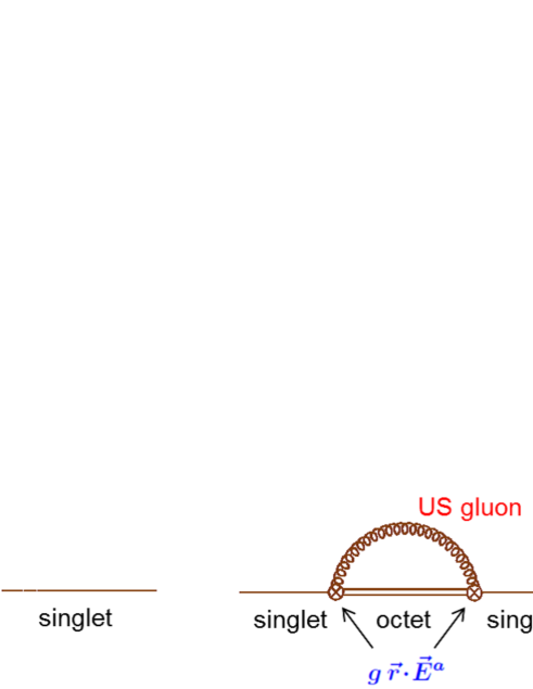
Figure 1: First two diagrams for the full propagator of $S$ in multipole expansion in pNRQCD.

The full propagator, in multipole expansion in $\vec{r}$, is given by the diagrams in Fig. 1. The first diagram represents the zeroth-order propagator of $S$, which is simply $1/[E-\hat{H}_{S}+i0]$. Hence, its pole positions can be computed by ordinary perturbation theory of quantum mechanics using $\hat{H}_{S}$ up to NNNLO. The LO Hamiltonian is that of the Coulomb system. The perturbative corrections are given by the familiar formula:

$$\delta E_{n}=\left<{n}\,\right|(\hat{H}_{S})_{\rm NLO}\left|\,{n}\,\right>+\sum_{i\neq n}\frac{|\left<{n}\,\right|(\hat{H}_{S})_{\rm NLO}\left|\,{i}\,\right>|^{2}}{E_{n}-E_{i}}+\cdots\,.$$ (2)

Each term of the perturbative corrections can be straightforwardly converted to an infinite sum form using a known infinite sum representation of the Coulomb Green function.

The second diagram represents emission and reabsorption of an ultrasoft gluon via dipole interaction in eq. (1). This contribution is the same as Lamb shift in QED and contains UV divergences. The divergences are canceled by IR divergences contained in the Hamiltonian at NNNLO, $(\hat{H}_{S})_{\rm N^{3}LO}$, such that the sum of the two diagrams is finite. We now explain key aspects in the evaluation of contribution of each diagram in Fig. 1.

2.1 Breakdown of infinite sum to finite sums (and known transcendental numbers)

Let us explain the new technology to evaluate infinite sums in the evaluation of the first diagram. We take the following sum as an example:

$$A(n,\ell)=\sum_{k=1}^{\infty}\frac{(n-\ell+k-1)!}{(n+\ell+k)!\,k^{3}}.$$ (3)

This sum appears as a part of the NNLO corrections to the spectrum. We have devised a new method to reduce this type of infinite sums to a combination of transcendental numbers [such as $\zeta(2)=\pi^{2}/6$, $\zeta(3)$, etc.], rational numbers and a finite sum [6].

By partial fractioning, the product over the magnetic quantum number $m$ can be written as

$$\frac{(n-\ell+k-1)!}{(n+\ell+k)!}=\prod_{m=-\ell}^{\ell}\frac{1}{n+k+m}=\sum_{m=-\ell}^{\ell}\frac{R(\ell,m)}{n+k+m},$$ (4)

where the residue is given by

$$R(\ell,m)=\frac{(-1)^{\ell-m}}{(\ell+m)!(\ell-m)!}\,.$$ (5)

Now we can reduce the sum eq. (3) using eq. (4) and

$$\sum_{k=1}^{\infty}\frac{1}{(k+i)\,k^{3}}=\frac{\zeta(3)}{i}-\frac{\zeta(2)}{i^{2}}+\frac{S_{1}(i)}{i^{3}}\,.$$ (6)

[$S_{1}(i)=\sum_{k=1}^{i}\frac{1}{k}$ denotes the harmonic sum.]

To evaluate sums such as the one in eq (6), there exists a general algorithm [9] (see also [10]) which can evaluate, e.g.,

$$f(i)=\sum_{k=1}^{\infty}\sum_{m=1}^{\infty}\frac{(-1)^{m-k}}{(k+i)^{2}(k+m+i)(m+2i+1)}$$ (7)

by reducing it to a combination of nested sums

$$Z\left(n_{\rm max};\{b_{j}\};\{\lambda_{j}\}\right)=\!\!\!\!\!\!\!\!\!\!\!\!\!\!\!\sum_{n_{\rm max}>n_{1}>n_{2}>\cdots>n_{N}>0}\frac{\lambda_{1}^{n_{1}}\lambda_{2}^{n_{2}}\cdots\lambda_{N}^{n_{N}}}{n_{1}^{b_{1}}n_{2}^{b_{2}}\cdots n_{N}^{b_{N}}},~{}~{}~{}~{}~{}~{}~{}b_{j}\in\mathbb{N},~{}\lambda_{j}\in\mbox{roots of unity},$$ (8)

where $n_{\rm max}=i$ or $\infty$. In fact, as a factor in the denomanator on the RHS of eq. (7) any linear polynomial of internal and external indices can appear, while any roots of unity can appear in the numerator. The algorithm utilizes the fact that the summand of $f(i)$ can be brought to a form which is invariant under the shift of the indices, $i\to i+\Delta i$, $k\to k+\Delta k$, $m\to m+\Delta m$. Then it is easy to see that, by taking a difference equation of $f(i)$, the bulk of the sum gets canceled and only “surface terms” with one summation less remain. By repeating this procedure recursively and summing back, one can render $f(i)$ to a combination of nested sums, which can be evaluated in terms of known transcendental numbers, rational numbers and finite sums.

2.2 Algebraic derivation of US correction (QCD Bethe log)

We show how to compute the second diagram of Fig. 1 algebraically [6]. The diagram corresponds to the one-loop self-energy of the singlet field $S$ and is given by

$$E^{us}_{n\ell}=-ig^{2}\mu^{2\epsilon}\frac{T_{F}}{N_{C}}\int_{0}^{\infty}dt\left\langle\vec{r}\cdot\vec{E}^{a}(t,\vec{0})\,\exp\left[-i(\hat{H}_{O}^{(d)}-E_{n,C}^{(d)})t\right]\vec{r}\cdot\vec{E}^{a}(0,\vec{0})\right\rangle_{n\ell}.$$ (9)

$\langle\cdots\rangle_{n\ell}$ denotes the expectation value taken with respect to the (external) energy eigenstate $(n,\ell)$ of the singlet Hamiltonian $H_{S}^{(d)}$ in $d$ dimensions. We employ the dimensional regularization with $d=D-1=3-2\epsilon$. $E_{n,C}^{(d)}=-\frac{C_{F}^{2}\alpha_{s}^{2}}{4n^{2}}m+{\cal O}(\epsilon)$ denotes the (leading-order) energy eigenvalue of $H_{S}^{(d)}$. We need to keep $\epsilon=(3-d)/2$ non-zero until we extract the UV divergences of $E^{us}_{n\ell}$ explicitly.

The correlation function of the color electric field can be evaluated using the gluon propagator of the ordinary Feynman rules as

$$\left\langle E^{ia}(t,\vec{0})E^{ja}(0,\vec{0})\right\rangle=-i\delta^{aa}\int\frac{d^{D}k}{(2\pi)^{D}}\,\frac{e^{ik_{0}t}}{k^{2}+i0}\,\left(k^{i}k^{j}-k_{0}^{2}\delta^{ij}\right)~{}+~{}{\cal O}(\alpha_{s}).$$ (10)

After integrating over $t$ we obtain

$$E^{us}_{n\ell}=\frac{1}{2}C_{F}g^{2}\mu^{2\epsilon}\,\frac{1-d}{d}\,C(d)\,\left\langle r^{i}\left(\hat{H}_{O}^{(d)}-E_{n,C}^{(d)}\right)^{d}r^{i}\right\rangle_{n\ell}.$$ (11)

$C(d)$ is expressed in terms of Gamma functions and includes $1/\epsilon$ pole due to the UV divergence of the one-loop integral. Therefore, we need the other factors up to order $\epsilon$.

We may expand $(\hat{H}_{O}^{(d)}-E_{n,C}^{(d)})^{3-2\epsilon}\approx(\hat{H}_{O}^{(d)}-E_{n,C}^{(d)})^{3}[1-2\epsilon\log(\hat{H}_{O}^{(3)}-E_{n,C}^{(3)})]$ and write

$$\mu^{2\epsilon}\left\langle r^{i}\left(\hat{H}_{O}^{(d)}-E_{n,C}^{(d)}\right)^{d}r^{i}\right\rangle_{n\ell}=\left\langle X-2\epsilon\,r^{i}\left(\hat{H}_{O}^{(3)}-E_{n,C}^{(3)}\right)^{3}\log\left(\frac{\hat{H}_{O}^{(3)}-E_{n,C}^{(3)}}{\mu}\right)r^{i}\right\rangle_{n\ell}$$

$$~{}~{}~{}~{}~{}~{}~{}~{}~{}~{}~{}~{}~{}~{}~{}~{}~{}~{}~{}~{}~{}~{}~{}~{}~{}~{}~{}~{}~{}~{}~{}~{}~{}~{}~{}~{}~{}~{}~{}~{}~{}~{}~{}~{}~{}~{}~{}~{}+{\cal O}(\epsilon^{2})$$ (12)

with

$$\textstyle X=r^{i}\bigl{(}\hat{H}_{O}^{(d)}\bigr{)}^{3}r^{i}-\frac{3}{2}\left\{\hat{H}_{S}^{(d)},r^{i}\bigl{(}\hat{H}_{O}^{(d)}\bigr{)}^{2}r^{i}\right\}+\frac{3}{2}\left\{\bigl{(}\hat{H}_{S}^{(d)}\bigr{)}^{2},r^{i}\hat{H}_{O}^{(d)}r^{i}\right\}-\frac{1}{2}\left\{\bigl{(}\hat{H}_{S}^{(d)}\bigr{)}^{3},\vec{r}^{\,2}\right\},$$ (13)

where we have replaced $E_{n,C}^{(d)}$ by the singlet Hamiltonian inside the expectation value, taking into account ordering of the operators. We can then use the commutation relation $[r_{i},p_{j}]=i\delta_{ij}$ and $\left<{n}\,\right|[\hat{H}^{(d)}_{S},{\cal O}]\left|\,{n}\,\right>=0$, which hold for general $d$, to simplify $X$, and we obtain an operator $\hat{H}^{us}$, in which the $1/\epsilon$ terms and finite terms are explicitly separated:

$$E^{us}_{n\ell}=\left\langle\hat{H}^{us}\right\rangle_{n\ell}-\frac{2C_{F}\alpha_{s}}{3\pi}\left\langle r^{i}\left(H_{O}^{(3)}-E_{n,C}^{(3)}\right)^{3}\log\left(\frac{H_{O}^{(3)}-E_{n,C}^{(3)}}{{\mu}}\right)r^{i}\right\rangle_{n\ell}.$$ (14)

The $1/\epsilon$ part of $\hat{H}^{us}$ exactly cancels the $1/\epsilon$ part of $(\hat{H}_{S})_{\rm N^{3}LO}$. The second term on the RHS represents the QCD analogue of the “Bethe logarithm” in Lamb shift.

This is the algebraic derivation of the second diagram, and the result agrees with the previously known result. The original derivation [8] was based on diagrammatic analyses, which requires manipulation of vertices and propagators among a set of Feynman diagrams, using the equation of motion, etc. In general the algebraic derivation would be more tractable for non-experts.

3 Physics predictions

The scale dependence of the energy level of the lowest-lying spin-one quarkonium state is shown in Fig. 2.

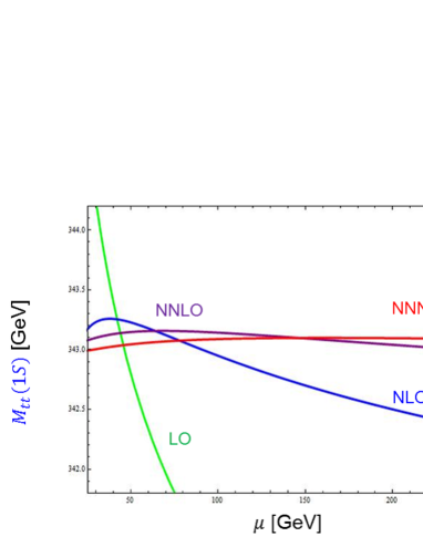
Figure 2: Renormalization-scale dependence of the energy level of the $t\bar{t}(1S)$ state.

The displayed figure is the case of the (would-be) $t\bar{t}(1S)$ state, and in the cases of the other heavy quarkonium $1S$ states the dependences are qualitatively similar. As can be seen, better stability is obtained as we include higher-order corrections. One can also verify that the perturbative series is converging fairly well around the scale where the $\mu$ dependence becomes flat (minimal-sensitivity scale). It is crucial to use a short-distance mass of the heavy quark to realize these nice features, and in particular the $\overline{\rm MS}$ mass shows the best stability and convergence [11]. (In this regard, the recent computation of the four-loop pole-$\overline{\rm MS}$ mass relation [12] is highly appreciated.)

We show in Fig. 4 a (preliminary) prediction for the bottomonium spectrum in perturbative QCD (red points) compared with the experimental data (black points).

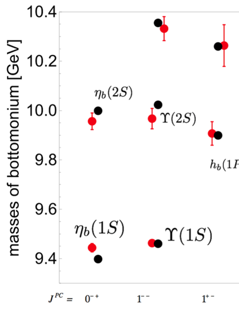
Figure 3: Comparison of the prediction of bottomonium spectrum by perturbative QCD and the experimental data. The prediction does not include non-zero charm-mass effects inside loops. (This figure was made by G. Mishima.)

Experimental errors are smaller than the black points, while theoretical error estimates are shown by red bars. The bottom quark $\overline{\rm MS}$ mass $\overline{m}_{b}$ is fixed on the $\Upsilon(1S)$ state and the value of $\alpha_{s}(M_{Z})$ to the PDG value. The prediction [13] does not include non-zero charm-mass effects inside loops in this figure. The prediction is in reasonable agreement with the experimental data, with essentially only $\overline{m}_{b}$ as the adjustable input parameter.

We can compare the perturbative QCD predictions and the experimental data for the $1S$ energy levels and determine the $\overline{\rm MS}$ masses of charm and bottom quarks, $\overline{m}_{c}$ and $\overline{m}_{b}$. This is shown in Fig. 4.

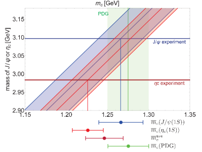
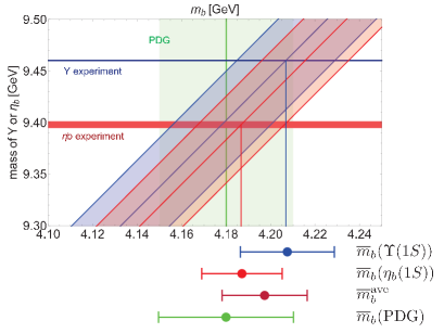
Figure 4: Determination of $\overline{\rm MS}$ masses $\overline{m}_{c}$ and $\overline{m}_{b}$ [14]. Horizontal (vertical) axes represent $\overline{m}_{c,b}$ (mass of charmonium/bottomonium $1S$ state). Horizontal narrow bands show the experimental data with errors. Diagonal bands show the perturbative QCD predictions with errors as functions of $\overline{m}_{c,b}$. Determined $\overline{m}_{c,b}$ with error bars are shown below the plot. For comparison, the PDG values are also shown.

From the average of the values determined from the vector and scalar $1S$ states, we obtain [14] $\overline{m}_{c}=1246\pm 2(d_{3})\pm 4(\alpha_{s})\pm 23({\rm h.o.})~{}{\rm MeV}$ and $\overline{m}_{b}=4197\pm 2(d_{3})\pm 6(\alpha_{s})\pm 20({\rm h.o.})\pm 5(m_{c})~{}{\rm MeV}$, which agree with the current Particle Data Group values. The error estimates are based on standard methods for estimating perturbative uncertainties. Thus, the agreement suggests that non-perturbative corrections to these systems are (at most) comparable in size with the perturbative uncertainties, which is also consistent with renormalon analyses.

4 Challenge: Analytic evaluation of $a_{3}$ (3-loop QCD potential)

Currently the three-loop correction to the static QCD potential is known only numerically [15]. There remain three necessary expansion coefficients in $\epsilon$ of the master integrals whose analytical values are still unknown [16]. One of them is an expansion coefficient of the integral given by the diagram in Fig. 5.

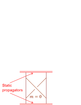
Figure 5: Diagram whose expansion coefficient is not known analytically. Single lines denote relativistic massless propagators, while double lines represent static propagators.

Let us explain the status of this coefficient. This expansion coefficient is reduced to the form

$$M_{40}^{(1)}=\sum_{k}r_{k}\,\,Z\!\left(\infty;\{b_{j}^{(k)}\};\{\lambda_{j}^{(k)}\}\right)+C_{0}\,,$$ (15)

namely, as a sum of generalized multiple zeta values (MZVs) (with rational number coefficients $r_{k}$) and an unknown constant $C_{0}$. Here, generalized MZV is defined as

$$Z\left(\infty;\{b_{j}\};\{\lambda_{j}\}\right)=\!\!\!\!\!\sum_{n_{1}>n_{2}>\cdots>n_{N}>0}\frac{\lambda_{1}^{n_{1}}\lambda_{2}^{n_{2}}\cdots\lambda_{N}^{n_{N}}}{n_{1}^{b_{1}}n_{2}^{b_{2}}\cdots n_{N}^{b_{N}}},~{}~{}~{}~{}~{}~{}~{}~{}b_{j}\in\mathbb{N},~{}\lambda_{j}\in\mathbb{C}.$$ (16)

The following integral includes the constant $C_{0}$ whose value has not been expressed in terms of MZVs up to now:

$$\int^{\Lambda}_{0}dx\,\frac{1}{\sqrt{x}\sqrt{1-4x}}\int_{1/4}^{x}dy\,\frac{1+2y}{y\sqrt{1-y}\sqrt{1-4y}}\int^{y}_{1}dz\,\frac{{\rm Arctan}\,z}{z\sqrt{1-z}}$$

$$~{}~{}=C_{2}\,\log^{2}\Lambda+C_{1}\,\log\Lambda+C_{0}+{\cal O}\Bigl{(}\frac{1}{\Lambda}\log^{n}\Lambda\Bigr{)}~{}~{}~{}~{}~{}~{}\mbox{as~{}~{}$\Lambda\to\infty$}.$$ (17)

We consider the limit $\Lambda\to\infty$ and extract the coefficients $C_{0},C_{1},C_{2}$ as above. $C_{2}$ and $C_{1}$ can be expressed by MZVs, which is a result of a non-trivial analysis. The constant $C_{0}$ has not been expressed by MZVs and its nature is still unknown. Similar nested integrals with square roots have also been investigated in this workshop. We would like to invite our colleagues to reveal the nature of $C_{0}$.

5 Summary

As demonstrated in this talk, non-relativistic bound state theory for QCD (also for QED) has become fairly mature and amenable to a textbook-level understanding and computation. A number of recent computations use pNRQCD EFT to organize perturbative expansions systematically.

In the computation of NNNLO heavy quarkonium spectrum we applied a new technology for evaluating multiple sums (which may be useful in other applications also) and performed all computation arithmetically in contrast to the previous approach which involved diagrammatic analyses. We also note that after many years of endeavor the computation of the NNNLO corrections to the quark pair-production cross section near threshold in $e^{+}e^{-}$ collisions has recently been completed [17]. One example of the remaining theoretical challenges is an analytic evaluation of the three-loop correction to the static QCD potential. It involves evaluation of a new type of nested integral with square roots.

We demonstrated some physics applications of the NNNLO heavy quarkonium spectrum. The prediction shows stability and convergence expected for a legitimate perturbative prediction. The prediction of the bottomonium spectrum is in reasonable agreement with the experimental data, in particular by fixing $\alpha_{s}(M_{Z})$ at the PDG value, with $\overline{m}_{b}$ as the only adjustable input parameter. We further determined the $\overline{\rm MS}$ masses $\overline{m}_{c}$ and $\overline{m}_{b}$ by comparing the experimental data for $J/\psi(1S),\eta_{c}(1S)$ and $\Upsilon(1S),\eta_{b}(1S)$ masses with the predictions of perturbative QCD. The obtained values of each mass from the different spin states are consistent with each other, as well as with the current PDG value which is determined from a wide variety of observables. These features suggest that non-perturbative corrections to these systems are comparable in size with the perturbative uncertainties and therefore under good theoretical control. Considering the role played by perturbative QCD in the present and future precision physics, this observation is fairly encouraging.

References

- [1] N. Brambilla et al. [Quarkonium Working Group Collaboration], “Heavy quarkonium physics,” hep-ph/0412158; N. Brambilla et al., “Heavy quarkonium: progress, puzzles, and opportunities,” Eur. Phys. J. C 71 (2011) 1534 [arXiv:1010.5827 [hep-ph]].
- [2] A. Pineda and J. Soto, Nucl. Phys. Proc. Suppl. 64, 428 (1998); N. Brambilla, A. Pineda, J. Soto and A. Vairo, Nucl. Phys. B 566, 275 (2000).
- [3] M. E. Luke, A. V. Manohar and I. Z. Rothstein, Phys. Rev. D 61, 074025 (2000).
- [4] M. Beneke and V. A. Smirnov, Nucl. Phys. B 522 (1998) 321 [hep-ph/9711391].
- [5] M. Beneke, Y. Kiyo and K. Schuller, Nucl. Phys. B 714 (2005) 67; A. A. Penin, V. A. Smirnov and M. Steinhauser, Nucl. Phys. B 716 (2005) 303.
- [6] Y. Kiyo and Y. Sumino, Nucl. Phys. B 889 (2014) 156 [arXiv:1408.5590 [hep-ph]].
- [7] C. Peset, A. Pineda and M. Stahlhofen, JHEP 1605 (2016) 017 [arXiv:1511.08210 [hep-ph]].
- [8] B. A. Kniehl, A. A. Penin, V. A. Smirnov and M. Steinhauser, Nucl. Phys. B 635 (2002) 357.
- [9] C. Anzai and Y. Sumino, J. Math. Phys. 54 (2013) 033514 [arXiv:1211.5204 [hep-th]].
- [10] J. Blumlein, S. Klein, C. Schneider and F. Stan, “A Symbolic Summation Approach to Feynman Integral Calculus,” J. Symbolic Comput. 47 (2012) 1267-1289 [arXiv:1011.2656 [cs.SC]].
- [11] Y. Kiyo, G. Mishima and Y. Sumino, JHEP 1511 (2015) 084 [arXiv:1506.06542 [hep-ph]].
- [12] P. Marquard, A. V. Smirnov, V. A. Smirnov and M. Steinhauser, Phys. Rev. Lett. 114, 142002 (2015).
- [13] Y. Kiyo and Y. Sumino, Phys. Lett. B 730 (2014) 76 [arXiv:1309.6571 [hep-ph]].
- [14] Y. Kiyo, G. Mishima and Y. Sumino, Phys. Lett. B 752 (2016) 122 [arXiv:1510.07072 [hep-ph]].
- [15] C. Anzai, Y. Kiyo and Y. Sumino, Phys. Rev. Lett. 104, 112003 (2010) [arXiv:0911.4335 [hep-ph]]; A. V. Smirnov, V. A. Smirnov and M. Steinhauser, Phys. Rev. Lett. 104, 112002 (2010) [arXiv:0911.4742 [hep-ph]].
- [16] A. V. Smirnov, V. A. Smirnov and M. Steinhauser, PoS RADCOR 2009 (2010) 075 [arXiv:1001.2668 [hep-ph]].
- [17] M. Beneke, Y. Kiyo, P. Marquard, A. Penin, J. Piclum and M. Steinhauser, Phys. Rev. Lett. 115 (2015) no.19, 192001 [arXiv:1506.06864 [hep-ph]].