Non-Linearly Interacting Ghost Dark Energy in Brans-Dicke Cosmology

Abstract

In this paper we extend the form of interaction term into the non-linear regime in the ghost dark energy model. A general form of non-linear interaction term is presented and cosmic dynamic equations are obtained. Next, the model is detailed for two special choice of the non-linear interaction term. According to this the universe transits at suitable time ($z\sim 0.8$) from deceleration to acceleration phase which alleviate the coincidence problem. Squared sound speed analysis revealed that for one class of non-linear interaction term $v_{s}^{2}$ can gets positive. This point is an impact of the non-linear interaction term and we never find such behavior in non interacting and linearly interacting ghost dark energy models. Also statefinder parameters are introduced for this model and we found that for one class the model meets the $\Lambda CDM$ while in the second choice although the model approaches the $\Lambda CDM$ but never touch that.

I Introduction

QCD ghost dark energy (GDE) is one of models presented to solve the unexpected acceleration problem of the universeRie ; perl1 ; perl2 ; hanany ; spergel ; coll ; teg ; cole ; springel . This model is based on the Veneziano ghost scalar field which was presented to solve the so-called $U(1)$ problem veneziano . Taking a flat Minkowski background into account the ghost scalar filed does not show any physical effect to vacuum energy of spacetime. However, considering a curved or dynamic spacetime cancelation of the vacuum energy density will not be complete and there remains a small contribution to the energy density. Authors of urban ; ohta showed that in an expanding background this contribution can be written as $\Lambda^{3}_{QCD}H$, where H is the Hubble parameter and $\Lambda^{3}_{QCD}$ is QCD mass scale. Taking $\Lambda_{\rm QCD}\sim 100MeV$ and $H\sim 10^{-33}eV$ ,$\Lambda^{3}_{\rm QCD}H\sim(3\times 10^{-3}eV)$ which can alleviate the fine tuning problemohta . Beside this nice resolution of the fine tuning problem the GDE model is interesting because there is no need to add a new degree of freedom to current state of the physics literature. According to this form of energy density ,$\rho_{GDE}\sim H$, the ghost dark energy was proposed to solve acceleration problem. Cai et.al considered the cosmological consequences of this model of dark energy in CaiGhost . They constrained the parameters by observations and also discussed the cosmic dynamics. Also authors considered $v_{s}^{2}$ analysis and found signs of instability in the model. In ebrins , the authors considered $v_{s}^{2}$ analysis in details in presence and absence of the non-gravitational interaction which the results were in agreement with that of Cai et.al. Other features of the GDE energy are investigated. Sheykhi et.al presented a tachyon reconstruction of the model in shemov . In this paper the authors showed that the evolution of the ghost dark energy dominated universe can be reconstructed by a tachyon scalar field. The potential of the tachyon field are presented according to the GDE model. Quintessence relation to the GDE is also considered in sheykhi1 . A K-essence reconstruction of GDE is presented by A. R. Fernandez fernandez . The author discussed the kinetic k-essence function F(X) in a flat background.

Interacting models of dark energy, introduced in the literature by Wetterich in wett . They found a solution to the so-called ”coincidence problem” which simply asks that why the DE component becomes the dominant component at present time? The interaction between DM and DE energy can be considered observationally and theoretically. There are evidences which confirm a better consistency between observations and interacting models of DE in comparison with the non-interacting models. Examples are presented in interact1 ; oli . Also theoretically there is no reason against interaction between dark sector components. If one(or both)dark component does not interact with the rest of the universe then it would be conserved. What symmetry in system support such a conserved quantity? This question at present time due to lack of a underlying theory for DM and DE does not receive any answer. Then there is a lot of interest to models of DE which leave a chance of interaction between dark sectors of the universe. However, the form of interaction term is still a matter of choice and generally can be written as $Q\sim\Gamma f(\rho_{m},\rho_{D})$. In simplest level, $f$ can be taken as a linear function of energy densities. The choice $f=\rho_{m},\rho_{D},\rho_{m}+\rho_{D}$ is investigated widely in the literature Ame ; Zim ; wang1 . Also authors tried to extend the form of interaction term to non-linear regime. For example authors of, jian , showed that a product coupling, i.e., an interaction term which is proportional to the product of $\rho_{D}$, $\rho_{m}$ and $\rho_{D}+\rho_{m}$ can be consistent with observations. Next in arevalo , the authors tried a general form of non-linear interaction term and studied the cosmic dynamic of the universe in presence of such interaction term. For a special case of the non-linear interaction term they found analytic solutions which is consistent with the supernova type Ia (SNIa) data from the Union2 set. Another example can be seen in BD3 which the authors study DE models in presence of a non-linear interaction term from a dynamical system point of view. Our aim in this paper is to examine such non linear interaction term in BD framework in a two component universe filled with GDE and cold dark matter.

The Brans-Dicke theory of gravity was proposed in 1961 BD . This model modifies the Einstein’s gravity in a way admitting the so called ”Mach’s principle”. To this end , a new scalar degree of freedom is added to incoroporate the Mach’s principle. The Brans Dicke theory has passed experimental tests in the solar system bertotti . One can find more features of BD cosmology inBD1 ; BD2 .

We also find the statefinder parameters, in order to discriminate the model from the other dark energy models. The statefinder pair parameters $\{r,s\}$, introduced by Sahni et al Sahni:2002fz ; Alam:2003sc , is the geometrical diagnostic pair, which is constructed from the scale factor and its derivatives up to third order. This is a geometrical pair since it is constructed from the space-time metric directly. Hence, statefinder is more universal parameter to study the dark energy models than any other physical parameters. It is possible to construct a two dimensional space spanned by $r$ and $s$ which different trajectories in this plane corresponds to different dark energy models. Statefinder analysis for loop quantum cosmology and $f(T)$ gravity can be find respectively in SF1 ; SF2 . In SF3 , the statefinder parameters are constrained by observational data.

The rest of this paper is organized as follows. In the next section, we present the GDE model in the flat BD theory with a closed form of interaction ($Q$). The next section is devoted to the non-linearly interacting GDE model. In section IV, we discussed the statefinder analysis for non-linearly interacting model. We summarize our results in section V.

II Ghost dark energy in BD theory with linear interaction

The action of the Brans-Dicke gravity with one scalar field $\phi$ can be written as

$$I_{G}=-\frac{1}{16\pi}\int_{\mathcal{M}}d^{n+1}x\sqrt{-g}\left(\phi{R}-\frac{\omega}{\phi}(\nabla\phi)^{2}+{\cal L}(m)\right),$$ (1)

where ${R}$ is the scalar curvature, $\cal L$ is the Lagrangian density of the matter and $\omega$ is the BD constant. Governing field equations can be obtained by varying the action with respect to $g_{\mu\nu}$ and $\phi$. The results read

$$\phi\,G_{\mu\nu}=-8\pi T_{\mu\nu}^{M}-\frac{\omega}{\phi}\left(\phi_{,\mu}\phi_{,\nu}-\frac{1}{2}g_{\mu\nu}\phi_{,\lambda}\phi^{,\lambda}\right)-\phi_{;\mu;\nu}+g_{\mu\nu}\Box\phi,$$ (2)

$$\Box\phi=\frac{8\pi}{(n-1)\omega+n}T_{\lambda}^{M\,\lambda}.$$

One important point about BD theory is its varying gravitational constant $G$. In BD gravity the, $G^{-1}_{\mathrm{eff}}={2\pi\phi^{2}}/{\omega}$, where $G_{\mathrm{eff}}$ is the effective gravitational constant as long as the scalar field $\phi$ changes slowly.

Taking the Friedmann-Robertson-Walker (FRW) metric and above equations into account we obtain the BD cosmology field equations as

$$\frac{3}{4\omega}\phi^{2}\left(H^{2}+\frac{k}{a^{2}}\right)-\frac{1}{2}\dot{\phi}^{2}+\frac{3}{2\omega}H\dot{\phi}\phi=\rho_{M}+\rho_{D},$$ (3)

$$\frac{-1}{4\omega}\phi^{2}\left(2\frac{{\ddot{a}}}{a}+H^{2}+\frac{k}{a^{2}}\right)-\frac{1}{\omega}H\dot{\phi}\phi-\frac{1}{2\omega}\ddot{\phi}\phi-\frac{1}{2}\left(1+\frac{1}{\omega}\right)\dot{\phi}^{2}=p_{D},$$ (4)

$$\ddot{\phi}+3H\dot{\phi}-\frac{3}{2\omega}\left(\frac{{\ddot{a}}}{a}+H^{2}+\frac{k}{a^{2}}\right)\phi=0,$$ (5)

where $a(t)$ is the scale factor, and $k$ is the curvature parameter with $k=-1,0,1$ corresponding to open, flat, and closed universes, respectively. Also $H=\dot{a}/a$, is the Hubble parameter, $\rho_{D}$ and $p_{D}$ are, the energy density and pressure of the dark energy respectively and $\rho_{M}$, is the dark matter density while we take a pressureless dark matter ($p_{M}=0$).

The energy conservation equations for DE and pressureless DM in presence of interaction read

$$\dot{\rho}_{D}+3H\rho_{D}(1+w_{D})=-Q,$$ (6)

$$\dot{\rho}_{M}+3H\rho_{M}=Q,$$ (7)

where $w_{D}=\frac{p_{D}}{\rho_{D}}$ is the equation of state parameter of dark energy and $Q$ denote the interaction between DE and DM components. Summing above equations one obtains

$$\dot{\rho}+3H(\rho+p)=0,$$ (8)

where $\rho=\rho_{D}+\rho_{M}$ and $p=p_{D}+p_{M}=p_{D}$. Above equations shows that although the presence of interaction term allows transition of energy between two components but the total energy content is still conserved. It is worth to note that in this paper we ignore the radiation contribution to the energy content due to its smallness.

Here our aim is to consider an interacting version of GDE in a flat background in the BD framework. The ghost dark energy density isohta

$$\rho_{D}=\Lambda_{\rm QCD}^{3}H,$$ (9)

where $\Lambda_{\rm QCD}$ is QCD mass scale. With $\Lambda_{\rm QCD}\sim 100MeV$ and $H\sim 10^{-33}eV$ , $\Lambda^{3}_{\rm QCD}H$ gives the right order of magnitude $\sim(3\times 10^{-3}eV)$ for the observed dark energy density ohta .

Adding above relation to the BD cosmology Eqs.(3-5),we still have a problem in analyzing the system. The system of equations is not closed and we need to introduce more relations. To this end, according to already presented papers in the literature we consider a power law relation between BD scalar field $\phi$ and scale factor as

$$\phi\propto a^{\varepsilon}.$$ (10)

There exist strong observational constraint on $\varepsilon$. Wu and Chen in wu using WMAP and SDSS data evaluated the rate of change in the gravitational constant $G$ and using this parameter found that $\varepsilon<0.01$. Also in this paper they presented a constraint on the BD constant $\omega$. They found that $\omega<-120.0$ or $\omega>97.8$ wu . A solar-system probe in bertotti reveals that $\omega>40000$ while a cosmic scale survey shows that $\omega$ is smaller than 40000 acqui . In another paper using local astronomical observations put a lower bound on $\omega$ Will .

Considering the ansatz (10) one finds

$$\frac{\dot{\phi}}{\phi}=\varepsilon\frac{\dot{a}}{a}=\varepsilon H.$$ (11)

Assuming above formula, the first Friedmann equation (3) in a flat background becomes

$$(1-\frac{2\omega}{3}\varepsilon^{2}+2\varepsilon) = \frac{4\omega}{3\phi^{2}H^{2}}(\rho_{D}+\rho_{M}),$$ (12)

$$\Rightarrow\gamma = \Omega_{D}+\Omega_{M}.$$ (13)

In writing above equation we used the following definitions

$$\Omega_{M} = \frac{\rho_{M}}{\rho_{\mathrm{cr}}}=\frac{4\omega\rho_{M}}{3\phi^{2}H^{2}},$$ (14)

$$\Omega_{D} = \frac{\rho_{D}}{\rho_{\mathrm{cr}}}=\frac{4\omega\rho_{D}}{3\phi^{2}H^{2}},$$ (15)

$$\gamma = 1-\frac{2\omega}{3}\varepsilon^{2}+2\varepsilon.$$ (16)

Taking time derivative from (9) we reach

$$\frac{\dot{\rho_{D}}}{\rho_{D}}=\frac{\dot{H}}{H}.$$ (17)

As we mentioned we would like to consider the GDE with non-linear interaction in a flat background ($k=\Omega_{k}=0$). Taking time derivative of (12) and dividing both side by $H^{2}$ one finds a relation for $\frac{\dot{H}}{H}$. Also doing a little algebra with (6), we get an equivalent for $\frac{\dot{\rho_{D}}}{\rho_{D}}$. Inserting these relations in (17), one can find

$$w_{D}=\frac{\gamma}{2\gamma-\Omega_{D}}\left[\frac{2\varepsilon}{3}-1-\frac{2Q}{3H\rho_{D}}\right].$$ (18)

Next, we turn to the deceleration parameter

$$q=-\frac{\ddot{a}}{aH^{2}}=-1-\frac{\dot{H}}{H^{2}}=\varepsilon+\frac{1}{2}+\frac{3}{2}\frac{\Omega_{D}w_{D}}{\gamma}.$$ (19)

Replacing relation (18) in above equation we get

$$q=\varepsilon+\frac{1}{2}+\frac{3\Omega_{D}}{2(2\gamma-\Omega_{D})}\left[\frac{2\varepsilon}{3}-1-\frac{2Q}{3H\rho_{D}}\right].$$ (20)

To give a complete set of equations of cosmic dynamics we should also bring dark energy density parameter evolution equation. To this end one can take a time derivative of (15) and after a little algebra reach

$$\frac{d\Omega_{D}}{d\ln a}=\frac{3\Omega_{D}}{2}\left[1-\frac{\Omega_{D}}{2\gamma-\Omega_{D}}(1+\frac{2Q}{3H\rho_{D}})+\frac{2\varepsilon}{3}\frac{2(\Omega_{D}-\gamma)}{2\gamma-\Omega_{D}}\right],$$ (21)

In order to find GR limit of above equations we should set $\varepsilon=0$ ($\omega\rightarrow\infty$) and $\gamma=1$. Taking GR limit of $w_{D},q$, evolution equation (21) and setting $Q=3b^{2}H(\rho_{D}+\rho_{m})$ we get

$$w_{D}=\frac{-1}{2-\Omega_{D}}\left[1+\frac{2b^{2}}{\Omega_{D}}\right],$$ (22)

$$q=\frac{1}{2}-\frac{3\Omega_{D}}{2(2-\Omega_{D})}\left[1+\frac{2b^{2}}{\Omega_{D}}\right],$$ (23)

$$\frac{d\Omega_{D}}{d\ln a}=\frac{3\Omega_{D}}{2}\left[1-\frac{\Omega_{D}}{2-\Omega_{D}}(1+\frac{2b^{2}}{\Omega_{D}})\right],$$ (24)

which exactly correspond to those obtained in sheykhi4 . Having the relations (18), (20) and (21) at hand we are ready insert any form of interactions and find the subsequent impacts on cosmic dynamics.

III Interacting Ghost dark energy with generalized interaction term in flat BD theory

Nature and origin of the dark energy and dark matter is still unknown. Thus there are a lot of features which usually are consequences of choices. One important example of this area is the interaction problem between dark components. When we model the recent acceleration of the universe through DE, it seems that in some features we get better agreement with observations if we consider an interaction between dark components. An example is evidences from galaxy cluster Abell A586 which show better agreement withe theoretical approach when there exist interaction between DE and DM interact1 . From theoretical view there is not any reason against interaction DM and DE. Thus many authors consider interacting models of DE. In one branch people start the the model with introduction of Lagrangians which leads to interacting models. Instances can be find in samisuji . So there is enough motivations observationally and theoretically to consider interacting models of DE($Q\neq 0$). Since there is not any underlying theory to inform us about the form of interaction term, then people usually consider this issue phenomenologically. One more helping point come from dimensional analysis which says that the interaction term should have a same dimension as energy density dimension. In simplest level people consider a linear relation proportional to $\rho_{D}$, $\rho_{M}$ or sum of them. However there still are many choices to be examined in this regard. There are examples of interacting models which the interaction term contains products of different energy components jian . As we mentioned in the introduction our aim in this note is to extend such ideas to a general case which includes more variety of these models. The form of interaction read

$$Q=3Hb^{2}\rho_{D}^{\alpha}\rho_{m}^{\beta}\rho^{\xi},$$ (25)

where $\rho=\rho_{m}+\rho_{D}$ and $b^{2}$ is coupling constant factor. The powers $\alpha$, $\beta$ and $\xi$ specify the form of the interaction. Dimensional analysis constraint above equation through

$$\alpha+\beta+\xi=1.$$ (26)

This form of interaction with above constraint includes a variety choices in the literature. For example , for ($\alpha$; $\beta$; $\xi$) = (1; 0; 0) one find $Q\propto\rho_{D}$ and for ($\alpha$; $\beta$; $\xi$)= (0; 1;0) the case $Q\propto\rho_{m}$ is retrieved. This form of interaction term leave a chance of analytic solutions in some casesarevalo ; oliverose .

Taking the relation (26), it can be seen that

$$Q=3Hb^{2}\rho_{D}^{\alpha}\rho_{m}^{\beta}\rho^{-\alpha-\beta+1}.$$ (27)

To use above interaction term, we will rewrite it as

$$\frac{2Q}{3H\rho_{D}}=2b^{2}\gamma^{-\alpha-\beta+1}\Omega_{D}^{\alpha-1}\Omega_{m}^{\beta},$$ (28)

where in last step we used Eqs.(13). In order to obtain the cosmic dynamic equations with this interaction form we insert above relation in equations (18), (20) and (21). The result read

$$w_{D}=\frac{\gamma}{2\gamma-\Omega_{D}}\left[\frac{2\varepsilon}{3}-1-2b^{2}\gamma^{-\alpha-\beta+1}\Omega_{D}^{\alpha-1}\Omega_{m}^{\beta}\right],$$ (29)

$$q=\varepsilon+\frac{1}{2}+\frac{3\Omega_{D}}{2(2\gamma-\Omega_{D})}\left[\frac{2\varepsilon}{3}-1-2b^{2}\gamma^{-\alpha-\beta+1}\Omega_{D}^{\alpha-1}\Omega_{m}^{\beta}\right],$$ (30)

$$\frac{d\Omega_{D}}{d\ln a}=\frac{3\Omega_{D}}{2}\left[1-\frac{\Omega_{D}}{2\gamma-\Omega_{D}}(1+2b^{2}\gamma^{-\alpha-\beta+1}\Omega_{D}^{\alpha-1}\Omega_{m}^{\beta})+\frac{2\varepsilon}{3}\frac{2(\Omega_{D}-\gamma)}{2\gamma-\Omega_{D}}\right].$$ (31)

It is worth to mention that for choice $\alpha=\beta=0$, all above equations convert to the linear interaction relation which was presented at the end of previous section. Above equations reveals the impact of the non-linear interaction term on the cosmic dynamics. However, here we also consider the issue of stability against small perturbations in the background using the squared sound speed ($v_{s}^{2}$) analysis. In present time the universe is in a DE dominated stable phase then any sign of instability,$(v_{s}^{2}<0)$, can challenge the model. To this end we use

$$v_{s}^{2}=\frac{dP}{d\rho}=\frac{\dot{P}}{\dot{\rho}}=\frac{\rho}{\dot{\rho}}\dot{w}+w,$$ (32)

where $w$ is the effective EoS parameter. After a little algebra one finds

$$v_{s}^{2} = \frac{-4\Omega_{D}}{\big{(}(2\gamma-\Omega_{D})^{2}(\gamma-\Omega_{D})(-3{\gamma}^{-\beta-\alpha+1}{\Omega_{D}}^{\alpha-1}(\gamma-\Omega_{D})^{\beta}\Omega_{D}{b}^{2}+\Omega_{D}\,\epsilon+3\gamma-3\Omega_{D})\big{)}}\big{[}$$ (33)

$$\big{[} \frac{3}{2}\Omega_{D}^{2\alpha-1}\big{(}(\frac{\beta}{2}+\frac{\alpha}{2}-\frac{3}{2}){\Omega_{D}}^{2}-\gamma(\beta+\frac{3\alpha}{2}-\frac{7}{2})\Omega_{D}+\gamma^{2}(\alpha-2)\big{)}((\gamma-\Omega_{D})^{\beta})^{2}{b}^{4}(\gamma^{-\beta-\alpha+1})^{2}\big{]}+$$

$$\big{[} (\gamma-\Omega_{D})\Omega_{D}^{\alpha-1}(\gamma-\Omega_{D})^{\beta}\big{(}((\frac{\beta}{2}+\frac{\alpha}{2}-\frac{3}{2})\epsilon-\frac{3\beta}{4}-\frac{3\alpha}{4}+3){\Omega_{D}}^{2}-\gamma((\beta+\frac{3\alpha}{2}-2)\epsilon-\frac{3\beta}{2}-\frac{9\alpha}{4}+6)\Omega_{D}$$

$$+ {\gamma}^{2}(\epsilon\alpha-\frac{3\alpha}{2}+3)\big{)}{b}^{2}{\gamma}^{-\beta-\alpha+1}\big{]}-\frac{1}{3}(\gamma-\Omega_{D})((-\frac{\epsilon}{2}+\frac{3}{2}){\Omega_{D}}^{2}-3\gamma\Omega_{D}+{\gamma}^{2}(\epsilon+\frac{3}{2}))(\epsilon-\frac{3}{2})\big{]}.$$

In order to study the impact of the non-linear interaction, we discus two non-linear choice of the model.

III.1 $Q=3Hb^{2}\frac{\rho_{D}^{2}}{\rho}(\alpha=2,\beta=0)$

Plotting the density parameter equation versus the folding number $x=\ln{a}$, it is obvious that $\Omega_{D}$ tends to constant value rather than $1$. For larger $b$, more energy will be transferred to the matter component and final value of $\Omega_{D}$ will be smaller. However, for the DE component to catch the present value $\Omega_{D0}=0.69$, there will be an upper limit on the coupling constant $b$. One can see from Fig.(1), that the equation of state parameter crosses the phantom barrier. It is also obvious for this figure that for larger value of interaction parameter $b$ the EoS parameter takes more negative values and approaches a limiting value at late time.

Total fluid equation of state parameter is depicted in left part of Fig.(2). This figure indicates that the total EoS parameter approaches to $-1$ which reminds a big rip singularity for destination of the universe. Also it can be seen from this figure that in this model the universe enter the acceleration phase earlier for larger $b$.

Finally, the squared sound speed is studied to check for instability against small perturbations. $v_{s}^{2}$ is plotted against $x$ in right part of figure (2). This figure indicates that for all values of $b$, $v_{s}^{2}$ remains negative which shows a sign of instability. So this model suffers the stability problem although in other features the model seems to be consistent with observations.

Figure 1: In the left and right parts $\Omega_{D}$ and $w_{D}$ are plotted against $x$ for coupling form $Q=3Hb^{2}\frac{\rho_{D}^{2}}{\rho}$ respectively. In all figures through the paper we set $a_{0}=1,\varepsilon=0.002$ and $\omega=10000$

Figure 2: $w_{eff}$ and $v_{s}^{2}$ for case $(\alpha=2,\beta=0)$

III.2 $Q=3Hb^{2}\frac{\rho_{D}^{3}}{\rho^{2}}(\alpha=3,\beta=0)$

As mentioned in the previous case all features of the model can be consistent with observations but the squared sound speed analysis. So we will try another choice of (25) in this subsection. Also in this case the EoS parameter will cross the phantom line and approaches a constant value. Although the late limit of $w_{D}$ in this case is smaller than that of the previous case. In left part of Fig.(3), one can easily find that for larger values of the coupling parameter $b$ the universe transits to acceleration phase earlier. Also this figure indicates the possibility of a big rip as fate of the universe because the final limit of $w_{eff}$ is $-1$. Observationally, our universe seems to transits from deceleration to acceleration at the redshift value around $z>0.6$. It can be shown that for $b=0.5$ the universe transition from matter to DE dominated phase will happen at $x=-0.6(z\sim 0.8)$ which this point alleviate the coincidence problem. As we presented in the previous interaction form, one interesting point is the squared sound speed analysis which can reveals signs of instability in the current dark energy dominated universe. The previous case of interaction term was not able to provide a positive $v_{s}^{2}$ region around present time. Since, In present time the universe has stable, DE dominated phase of expansion then we need to find models which there is no signs of instability around present time. In the present form of interaction term there exists periods of time which $v_{s}^{2}$ gets positive values. The right part of Fig.(3), shows evolution of the $v_{s}^{2}$ against $x=\ln{a}$. It seems from this figure that for $b\geq 0.5$ there is a period of time which $v_{s}^{2}$ achieves positive values and after a finite era the $v_{s}^{2}$ will returns to the negative domain. We also found that this point couldn’t be seen in linearly interacting or non-interacting models of GDE in the BD framework and this is an important impact of the non-linear interaction term.

Figure 3: $w_{eff}$ and $v_{s}^{2}$ for case $(\alpha=3,\beta=0)$

IV The statefinder diagnostic

To describe the evolution of the Universe, we use two cosmological parameters H (the Hubble parameter) and q (the deceleration parameter), However these two parameters can not differentiate various dark energy models. In order to solve this problem, Sahni et al Sahni:2002fz have introduced a new geometrical diagnostic pair parameter $\{r,s\}$, termed as statefinder. $r$, $s$ are two dimensionless parameters which constructed from the scale factor and its derivatives up to the third order as

$$r=\frac{\dddot{a}}{aH^{3}}\,,\qquad s=\frac{r-1}{3\big{(}q-1/2\big{)}}\,.$$ (34)

$\{r,s\}$ are geometrical parameters since they constructed from the cosmic scale factor alone, so the statefinder is more universal than the physical variables which depend on the properties of physical fields describing dark energy models. In a flat $\Lambda$CDM model, the statefinder pair has fixed value $\{r,s\}=\{1,0\}$, also in the case of matter dominated universe (SCDM) one finds $\{r,s\}=\{1,1\}$ .

Note that $r$ can be expressed in terms of the Hubble and the deceleration parameters as Jawad:2014qoa $r=\ddot{H}/H^{3}-3q-2$. With the help of this equation and definition of the $q$ in (19), one can rewrite $r$ as

$$r=2q^{2}+q-\frac{\dot{q}}{H}\,.$$ (35)

Noting (30) for the general form of interactions, one finds that

$$\dot{q}=\frac{3}{2}\,\frac{\dot{\Omega}_{D}(2\gamma-\Omega_{D})+\dot{\Omega}_{D}\,\Omega_{D}}{(2\gamma-\Omega_{D})^{2}}\left(\frac{2\varepsilon}{3}-1-2b^{2}\gamma^{1-\alpha-\beta}\Omega_{D}^{\alpha-1}\Omega_{m}^{\beta}\right)-\frac{3\Omega_{D}}{2\gamma-\Omega_{D}}\left(b^{2}\gamma^{1-\alpha-\beta}(\alpha-1)\Omega_{D}^{\alpha-2}\dot{\Omega}_{D}\Omega_{m}^{\beta}\right),$$ (36)

where $\dot{\Omega}$ is given in (31). In the following we discuss the statefinder for some non-linear interactions between dark matter and the dark energy.

case 1): Linear interaction $Q=3Hb^{2}\rho$ .
The linear interaction can be obtained by set $\alpha=3\,,\beta=0$  in (25). In this case using (30)-(36) one can find statefinder parameters as

$$r = (2\gamma-\Omega_{D})^{-3}\big{[}\big{(}16\varepsilon^{2}+(24-48b^{2})\varepsilon+8+36b^{4}-36b^{2}\big{)}\gamma^{3}-3\Omega_{D}\big{(}\frac{4}{3}\varepsilon^{2}+(20-8b^{2})\varepsilon+7+9b^{4}-24b^{2}\big{)}\gamma^{2}$$ (37)

$$+ 6\Omega_{D}^{2}\big{(}4+5\varepsilon-6b^{2}+b^{2}\varepsilon-\frac{2}{3}\varepsilon^{2}\big{)}\gamma-10\Omega_{D}^{3}\big{]},$$

$$s = \big{[}3(2\gamma-\Omega_{D})^{2}(6b^{2}\gamma+3\Omega_{D}-4\varepsilon\gamma)\big{]}^{-1}\big{[}8(2\varepsilon+3-3b^{2})(-2\varepsilon\!+3b^{2})\gamma^{3}\!+6\Omega_{D}\big{(}\frac{4}{3}\varepsilon^{2}\!+(20-\!8b^{2})\varepsilon\!+\!3+9b^{4}\!-24b^{2}\big{)}\gamma^{2}$$ (38)

$$- 12\Omega_{D}^{2}\big{(}b^{2}\varepsilon-\frac{2}{3}\varepsilon^{2}-6b^{2}+3+5\varepsilon\big{)}\gamma+18\Omega_{D}^{3}\big{]}\,.$$

case 2): $Q=3Hb^{2}\frac{\rho_{D}^{3}}{\rho^{2}}$ .
In this case we should set $\alpha=3\,,\beta=0$ , so using (30)-(36) one can find

$$r = \big{[}\gamma(2\gamma-\Omega_{D})\big{]}^{-3}\big{[}(16\varepsilon^{2}+24\varepsilon+8)\gamma^{6}-4\Omega_{D}\big{(}\varepsilon^{2}+15\varepsilon+\frac{21}{4}\big{)}\gamma^{5}-4\Omega_{D}^{2}\big{(}\varepsilon^{2}-\frac{15}{2}\varepsilon-6\big{)}\gamma^{4}$$ (39)

$$- 84\Omega_{D}^{3}\big{(}b^{2}\varepsilon-\frac{3b^{2}}{14}+\frac{5}{42}\big{)}\gamma^{3}+78b^{2}\Omega_{D}^{4}\big{(}\varepsilon-\frac{3}{26}\big{)}\gamma^{2}-12b^{2}\Omega_{D}^{5}\big{(}\varepsilon+\frac{3}{4}\big{)}\gamma-18b^{4}\Omega_{D}^{6}\big{]},$$

$$s = \big{[}3\gamma(2\gamma-\Omega_{D})^{2}(6b^{2}\Omega_{D}^{3}+3\gamma^{2}\Omega_{D}-4\varepsilon\gamma^{3})\big{]}^{-1}\big{[}(-32\varepsilon^{2}-48\varepsilon)\gamma^{6}+8\Omega_{D}\big{(}\varepsilon^{2}\!+15\varepsilon+\frac{9}{4}\big{)}\gamma^{5}+8\Omega_{D}^{2}\big{(}\varepsilon^{2}\!-\frac{15}{2}\varepsilon-\frac{9}{2}\big{)}\gamma^{4}$$ (40)

$$+ 168\Omega_{D}^{3}\big{(}b^{2}\varepsilon-\frac{3b^{2}}{14}+\frac{3}{28}\big{)}\gamma^{3}-156b^{2}\Omega_{D}^{4}\big{(}\varepsilon-\frac{3}{26}\big{)}\gamma^{2}+24b^{2}\Omega_{D}^{5}\big{(}\varepsilon+\frac{3}{4}\big{)}\gamma+36b^{4}\Omega_{D}^{6}\big{]}\,.$$

case 3): $Q=3Hb^{2}\frac{\rho_{D}^{2}}{\rho}$ .
This non-linear interaction can be obtained by setting $\alpha=2\,,\beta=0$  in (25). In this case repeating (30)-(36) one can find statefinder parameters (due to briefness, we do not demonstrate $r$, $s$ in this case).
In figure (4) we have depicted the evolution of $\{r,s\}$ for the above cases. This figure shows that statefinder analysis can discriminate the models, where in all cases, curves lie in the region $r<1,s>0$ which implies the quintessence characteristic of the model Alam:2003sc , as on expected. In fig 4.b (non-linear interaction of case 2) the curve pass through the $\Lambda$CDM fixed point $\{r=1,s=0\}$ but in fig 4.a and 4.c, (linear interaction and non-linear interaction of case 3), the trajectories tend to the to the $\Lambda$CDM fixed point but do not touch it.

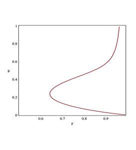
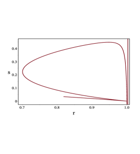
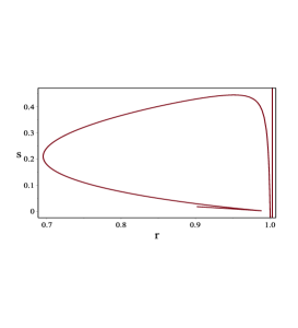
Figure 4: The evolution of statefinder parameter $r$ versus $s$ in the case of linear (Fig1a) and non-linear interactions (Fig1b,c) where we set $\gamma=1$, $\epsilon=.002$ and $b=0.1$ . All curves lie in the region of the quintessence models. In non-linear interaction of case 2 (Fig1b) the trajectory cross the $\Lambda$CDM fixed point. In the case of linear interaction and non-linear interaction of case 3 (Fig1c), the trajectories tend but do not touch the $\Lambda$CDM fixed point.

V Conclusion

In different models of dark energy the the form of interaction between dark matter and dark energy components has a linear dependency to $\rho_{m}$ and $rho_{D}$. In the absence of an underlying theory for DE and DM and also due to lack of observational evidences in this field, one can try the possibility of an interaction term with non-linear dependency to $\rho_{m}$ and $\rho_{m}$. In this paper we considered the consequences of such choices for interaction term in ghost dark energy model (GDE) in the Brans-Dicke framework.

To this goal we considered a non-linear form of interaction as $Q=3Hb^{2}\rho_{D}^{\alpha}\rho_{m}^{\beta}\rho^{-\alpha-\beta+1}$ and obtained the EoS parameter($w_{D}$), deceleration parameter ($q$) and evolution equation of the density parameter for GDE in BD framework in a flat background. These relations are presented for a general choice of the interaction term (arbitrary $\alpha$ and $\beta$). Next, we discussed two special choices of the interaction term. The first choice is $Q=3Hb^{2}\frac{\rho_{D}^{2}}{\rho}$. We obtained evolution of the density parameter ($\Omega_{D}$) in this case versus $x=\ln a$.Using this quantity we depicted the evolution of $w_{D},w_{eff}$ and $v_{s}^{2}$ versus $x$. The model sounds pretty well with what we expect. For example shows a long deceleration phase which ends at past and transits to a phase of acceleration which can solve the coincidence problem. However this model suffers the stability problem according to the squared sound speed ($v_{s}^{2}$) analysis. In this model the squared sound speed is always negative and never gets positive implying signs of instability against small perturbations in the background. Due to this reason we make another choice the interaction term to see if the ansatz of the non-linear interaction term is capable to remove such problem. Then we turn to the choice $Q=3Hb^{2}\frac{\rho_{D}^{3}}{\rho^{2}}$. In this choice of the interaction term all good features of the model are kept and the problem of negativity of the $v_{s}^{2}$ is removed. For suitable choice of coupling parameter $b$ we obtained a confined period of time which $v_{s}^{2}$ gets positive. However once again $v_{s}^{2}$ will enter negative domain which this point is in contrast with the same situation in the Einstein’s gravity ebnlgde . We have to emphasis here that in a GDE model in BD theory in non interacting case and also with linearly interacting case we never find such period of time which $v_{s}^{2}$ gets positive and this stage is an impact of the non-linear choice of the interaction term.

The statefinder diagnostic is also presented in the next section. In non-linear interaction of case ($Q=3Hb^{2}\frac{\rho_{D}^{3}}{\rho^{2}}$) the $\{r,s\}$ curve pass through the $\Lambda$CDM fixed point $\{r=1,s=0\}$ but for case $(Q=3Hb^{2}\frac{\rho_{D}^{2}}{\rho})$, the trajectory tend to the to the $\Lambda$CDM fixed point but do not touch it.

It is worth to mention that although the latter choice seems more consistent with what we expect a dependable model of DE but we need to take closer look at different features discriminating the model. Consistency with observational data and more subtle issues for non-linearly interacting models of GDE is now under investigation and will be addressed elsewhere.