Adiabatic Optimization Versus Diffusion Monte Carlo
Abstract
Most experimental and theoretical studies of adiabatic optimization use stoquastic Hamiltonians, whose ground states are expressible using only real nonnegative amplitudes. This raises a question as to whether classical Monte Carlo methods can simulate stoquastic adiabatic algorithms with polynomial overhead. Here, we analyze diffusion Monte Carlo algorithms. We argue that, based on differences between and normalized states, these algorithms suffer from certain obstructions preventing them from efficiently simulating stoquastic adiabatic evolution in generality. In practice however, we obtain good performance by introducing a method that we call Substochastic Monte Carlo. In fact, our simulations are good classical optimization algorithms in their own right, competitive with the best previously known heuristic solvers for MAX--SAT at .
I Introduction
While adiabatic quantum computation using general Hamiltonians has been proven to be universal for quantum computation [1], the vast majority of research so far, both experimental and theoretical, focuses on Hamiltonians in which all off-diagonal matrix elements are nonpositive. Such Hamiltonians were named stoquastic in [2]. By the Perron-Frobenius theorem, the ground state of a stoquastic Hamiltonian can always be expressed using only real nonnegative amplitudes. Consequently, in adiabatic computations, which stay in the ground state, interference effects are not manifest if the Hamiltonian is stoquastic. This raises some question as to whether adiabatic computation in the ground state of stoquastic Hamiltonians is capable of exponential speedup over classical randomized algorithms. Complexity-theoretic evidence obtained so far suggests that adiabatic quantum computation with stoquastic Hamiltonians is less powerful than universal quantum computers [2, 3] but does not resolve this question. Conventional wisdom among Monte Carlo practitioners states that Monte Carlo simulations of stoquastic adiabatic computation will not suffer from the sign problem and will therefore converge efficiently. If this could be turned into a theorem it would prove that stoquastic adiabatic computers are incapable of exponential speedup over classical computation.
Two of the major classes of Monte Carlo simulation algorithms are path integral Monte Carlo and diffusion Monte Carlo. In 2013, Hastings constructed a class of examples in which path integral Monte Carlo fails to efficiently simulate stoquastic adiabatic dynamics due to topological obstructions [4]. Diffusion Monte Carlo algorithms should not be affected by topological obstructions. We nevertheless find examples for which a nontopological obstruction prevents a diffusion Monte Carlo algorithm from efficiently simulating a stoquastic adiabatic process. On typical instances such simulations may nevertheless work well. In fact, we introduce a variant of diffusion Monte Carlo, which we call Substochastic Monte Carlo (SSMC), tailored to simulating stoquastic adiabatic processes. In practice, we find that this performs sufficiently well that SSMC simulations of adiabatic optimization are good classical optimization algorithms in their own right, competitive with the best previously known heuristic solvers for MAX--SAT at . Source code for our implementation is available at [5].
The relationship of quantum adiabatic optimization [6] and quantum annealing [7] to classical optimization heuristics and simulation methods has garnered a lot of attention. In particular, the most direct classical competitors to quantum adiabatic optimization appear to be gradient descent and simulated annealing, path integral Monte Carlo, and diffusion Monte Carlo. One can analytically address the performance of adiabatic optimization algorithms through adiabatic theorems [8, 9], which show that the runtime of adiabatic algorithms corresponding to Hamiltonians with eigenvalue gap is upper bounded by . Examples have been constructed in which adiabatic optimization exponentially outperforms simulated annealing and gradient descent [10]. Conversely, problems exist that can be solved in polynomial time by gradient descent but which have a corresponding exponentially small eigenvalue gap [11]. In the examples of [12, 13, 14], runtimes for path integral Monte Carlo and quantum adiabatic optimization have the same asymptotic scaling. However, the obstructions of [4] show that there exist cases where adiabatic optimization exponentially outperforms path integral Monte Carlo. Other informative analytical results on the effect of local minima on the performance of adiabatic optimization are given in [15, 16, 17, 18, 19, 20, 21, 22]. Experimental, numerical, and analytical evidence regarding the performance of quantum adiabatic optimization on combinatorial optimization problems such as MAX-SAT can be found in [6, 23, 24, 25, 26]. Some variants of the standard adiabatic optimization algorithm involving non-linear interpolation or non-stoquastic Hamiltonians are analyzed in [27, 28].
II Terminology and Notation
Let be a graph with vertex set and edge set . We presently restrict our attention to unweighted undirected graphs without self-loops. (Generalizing to weighted graphs is easy, however uninstructive for our current purposes.) By we denote the degree of vertex , that is, the number of edges with an endpoint . We use to denote the combinatorial Laplacian of , which is a matrix given by
| (1) |
As an example, consider the -dimensional hypercube graph . The vertices of may be labeled by bitstrings, and an edge connects a pair of bitstrings if and only if they differ by one bit. We write the corresponding combinatorial Laplacian in terms of the Pauli operators as
| (2) |
Here and throughout we use to denote the Pauli operators acting on qubit (tensored with identity on the remaining qubits). Aside from the (inconsequential) energy offset , the Laplacian is the most commonly used driving term for adiabatic optimization algorithms.
III Substochastic Monte Carlo
By Substochastic Monte Carlo (SSMC) we denote the class of classical population algorithms that simulate a time-dependent heat diffusion process driven by the same operator as the stoquastic adiabatic process. The particular variant of SSMC studied below can be viewed as either a form of diffusion Monte Carlo [29] or as a particular generalization of the “Go-With-The-Winners” algorithm of [30]. Consider a parametrized family of stoquastic Hamiltonians, which define an adiabatic algorithm by slowly varying from 0 to 1 according to some schedule . The corresponding imaginary-time dynamics
| (3) |
is a continuous time diffusion process. Correspondingly, at any given , the time-evolution operator is a substochastic matrix for any sufficiently small positive time step . Such substochastic matrices (i.e. square matrices with nonnegative entries such that each column sum is at most 1) generate substochastic random processes, in which total probability decreases. The lost probability is taken to represent the chance that the process stops or “dies”. SSMC is a Markov-Chain Monte Carlo method in which a population of random-walkers approximates the diffusion process on the graph given by this substochastic process conditioned on not having died.
While SSMC works with any family of stoquastic Hamiltonians, it is easiest to describe for
where is a combinatorial graph Laplacian, is a nonnegative diagonal operator, and and are suitable nonnegative scalar functions. When this is the case we may write
where is the diagonal operator of vertex degrees, and is the adjacency matrix of the graph. For a sufficiently small time step we approximate
which prescribes our transition probabilities. At time , the value is computed according to the schedule, and a walker on vertex would do precisely one of the following:
-
1.
step to vertex (where ), each with probability ,
-
2.
stay at vertex with probability ,
-
3.
or die with probability .
The expected proportion of walkers that die in a given timestep is where the expectation is computed with respect to the current ensemble population distribution at time . The proportion of the walkers that survive is . Conditioning on survival renormalizes our ensemble distribution, multiplying by . Combining this with the above produces our combined transition/renormalization matrix
| (4) |
If were constant in , this substochastic process converges to a quasistationary distribution (i.e. a distribution that is stationary except for exponentially decaying norm) that is proportional to the ground state of the original stoquastic Hamiltonian. Thus, one can attempt to simulate stoquastic adiabatic evolution using a substochastic classical random walk. The simplest idea would be to initialize the walkers into the ground state distribution of , which is typically the uniform distribution, and then track the instantaneous quasistationary distribution, as slowly increases from zero to one, by executing the Markov chain . (Here is the size of the timestep and .) However, one needs to introduce some process for replenishing the population of walkers. Otherwise, after a short time there are no walkers left and the simulation terminates.
There are a number of potential ways to replenish the walkers. We have found it effective to adaptively set an energy threshold throughout the time evolution such that walkers on sites with energy above the threshold are likely to die, whereas walkers on sites with energy below the threshold are likely to spawn offspring. According to (4) that threshold should be the mean energy of the population, . Specifically, in our scheme, at each timestep, a walker on vertex :
-
1.
steps to vertex (where ), each with probability ,
-
2.
stays at vertex with probability , or
-
3.
dies or spawns a new walker based on remaining probability .
We must have for the probabilities in Case 1 to make sense. A similar statement holds for Case 2, from which we derive
In particular, and we interpret Case 3 to be
-
3a.
if the walker dies with this probability, or
-
3b.
if then with probability the walker spawns an additional walker at vertex .
This choice of probabilities for spawning or dying ensures that the quasistationary distribution is proportional to the ground state of .
Note that the population size is itself a random variable. In theory, the threshold between dying and spawning is , however in practice one must adjust this to ensure the population size stays sufficiently close to a nominal value. This can be accomplished by introducing a feedback loop, which replaces with for some energy offset adaptively chosen based on the number of walkers. When the population size dwindles below the target value, is decreased. As one can see by examining the formulas defining 1, 2, 3a, and 3b, this replacement increases the likelihood for walkers to spawn, thereby replenishing the population. Conversely, when the number of walkers increases beyond the target population size, is increased, thereby increasing the likelihood for walkers to die.
Substochastic Monte Carlo can be viewed either as a method for simulating stoquastic adiabatic computation or as a method for solving discrete optimization problems. In the latter case, it is natural to ask why must be varied at all. In the typical case, and . Thus, where is the objective function that we seek to minimize. In this case, the pure diffusion process converges rapidly to the minimum energy state. However, in typical problems a good approximation to this diffusion process can generally only be achieved using an exponentially large population of walkers. A diagonal Hamiltonian implies that the probability for a walker to hop between vertices in SSMC is zero. The only remaining processes are death and spawning. If at least one walker is sitting at a minimum energy site, then death and spawning guarantee that the entire population converges to these sites, in agreement with the diffusion equation. However, in an optimization problem one does not initially know the optimum and therefore the initial distribution of walkers cannot depend upon knowledge of the minimum energy. For example, if the problem has a unique minimum energy vertex, the uniform distribution over all vertices has exponentially small overlap with the quasistationary distribution of , which is supported entirely by a single vertex. In this case, with only polynomially many walkers, it is exponentially unlikely that any walker is initially placed at the solution, and, due to lack of hopping, no walker arrives at the solution.
Intuitively, when SSMC is applied to optimization problems, the sweeping of from the graph Laplacian at to the diagonal matrix at serves a role loosely analogous to decreasing temperature in simulated annealing. Initially, when is small, the population of walkers explores widely. As is increased, the walkers become gradually more focused around the regions of the search space where the objective function has been found to take small values. If SSMC successfully tracks the quasi-stationary distribution then, after a given timestep, the walkers are distributed close to the quasi-stationary distribution of the current Hamiltonian . This then serves as the initial distribution for the next timestep with Hamiltonian . If is varied sufficiently slowly, then this initial distribution is close to the quasi-stationary distribution of , which facilitates convergence to the new quasistationary distribution.
If the substochastic Monte Carlo simulation successfully simulates the adiabatic process, then the final distribution of walkers will be proportional to the final ground state, which in the case of has support only on the minimum energy vertex. For solving an optimization problem defined by , this is sufficient though overkill; the optimum is found if at least one walker lands on the minimum energy vertex.
IV Non-Topological Obstructions
In this section we present a pair of stoquastic adiabatic processes which diffusion Monte Carlo algorithms such as SSMC will fail to efficiently simulate (with a stronger notion of failure in the second, more elaborate, example). Previously, [4] gave examples of stoquastic adiabatic processes that have polynomial eigenvalue gap but path integral Monte Carlo simulations of these processes take exponential time to converge. Loosely speaking, the failure of convergence was due to topological obstructions around which the worldlines can get tangled. In diffusion Monte Carlo algorithms, such as SSMC, there are no world lines, and correspondingly no susceptibility to these topological obstructions. Instead, our examples exhibit a different kind of obstruction, exploiting the fact that diffusion Monte Carlo simulations track the probability distribution proportional to the ground state amplitudes rather than the squared amplitudes. Our examples are inspired by the fourth counterexample given in §3.4 of [4], in which a discrepancy between the and -normalized wavefunctions is exploited to demonstrate exponential convergence time for a path integral Monte Carlo simulation with open boundary conditions.
For , let be some stoquastic Hamiltonian acting on a Hilbert space whose basis states can be equated with the vertices of some graph. Let denote the ground state of . Diffusion Monte Carlo algorithms (including SSMC) perform random walks designed to ensure that a population of random walkers converges to the probability distribution on directly proportional to the ground state . That is,
| (5) |
The stoquasticity of ensures that is always real and nonnegative, and consequently that is a valid probability distribution. In contrast, the probability distribution sampled from by performing a measurement on the quantum ground state of the adiabatic process is
| (6) |
In exponentially large Hilbert spaces there can be vertices such that
is polynomial but is exponentially
small. The idea behind our examples is to exploit this discrepancy to
design polynomial-time stoquastic adiabatic processes that the
corresponding diffusion Monte Carlo simulations will fail to
efficiently simulate.
Example 0: Consider the hypercube on qubits, and let
be the hypercube graph Laplacian, as described in
(2). Consider the stoquastic adiabatic Hamiltonian
| (7) |
where is the Hamming weight potential. That is,
| (8) |
where denotes the Hamming weight of bit string , i.e. the number of ones. (In terms of Pauli operators .) By the straightforward calculation given in Appendix A, one finds that by choosing
| (9) |
one obtains a ground state probability distribution that has
| (10) |
and therefore
| (11) |
whereas the corresponding distribution of random walkers behaves as
| (12) |
The minimum eigenvalue gap of occurs at and is equal to . Thus, this already constitutes an example where adiabatically evolving according to with varying from to over a polynomial duration and then measuring in the computational basis yields the minimum potential with constant probability, whereas diffusion Monte Carlo algorithms have subexponentially small probability of querying the minimum. This is not an especially compelling example, because SSMC may nevertheless efficiently converge to the probability distribution . That is, Example 0 disproves the naive hypothesis that if a measurement of an adiabatic process consistently yields the minimum of a potential in polynomial time, then so does SSMC. This, however, reflects only the exponential divergence in the and norms and does not disprove the following more nuanced hypothesis.
Hypothesis 1.
For all let be a stoquastic Hamiltonian with ground state and eigenvalue gap . Let . There exist polynomials such that with timesteps and walkers, SSMC tracks a probability distribution -close to .
We can disprove this hypothesis with the following, slightly more
elaborate example.
Example 1: Consider the Hamiltonian
| (13) |
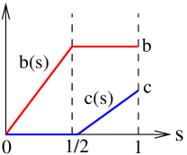
where and are as in Example 0 and is the projector onto the all zeros bitstring. The “annealing schedule” for is given by
| (16) | |||||
| (19) |
as illustrated in Figure 1. The constant is chosen as in (9).
As proven in Appendix B
| (20) |
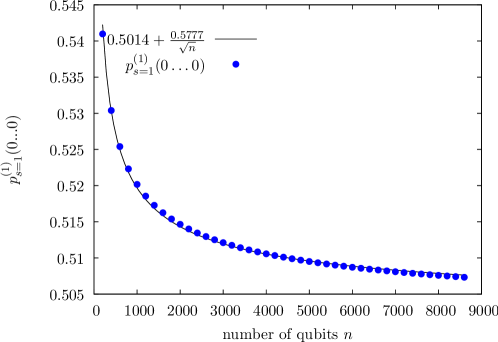
for any . The spectrum for recapitulates the spectrum of example 0. Thus, the minimum eigenvalue gap over the full adiabatic process occurs at and is given by . Consequently, the quantum adiabatic implementation of this process runs in polynomial time. By choosing sufficiently large we can ensure that is . Specifically, one finds numerically that by choosing one obtains
| (21) |
as shown in Figure 2. Thus, to satisfy Hypothesis 1, the walkers would have to end up at in a probability distribution with probability approximately at the all zeros string. However, from the analysis of Example 0, we know that at the walkers have a distribution in which the probability to be at the all zeros string is of order . Thus, with high likelihood, no walkers will land on the all zeros string until the number of timesteps times the number of walkers approaches . Until this happens it is impossible for the distribution of walkers to be affected by the change in the potential at the all zeros string that is occurring from to ; no walkers have landed there, and the diffusion Monte Carlo algorithm has therefore never queried the value of the potential at that site.
V Empirical Performance of Substochastic Monte Carlo
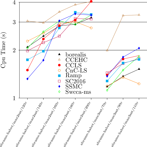
While highly structured problems may lead to obstructions, as in the previous section, unstructured and random problems are not likely to see these. There are numerous benchmarks of random problems available; here we provide results of SSMC and seven other solvers on a selection of unweighted random MAX-SAT problems from the 2016 MAX-SAT evaluation [31]. We omitted solvers that did not solve every problem instance in these categories. Also we do not show results on the high-girth examples of this benchmark as several of the algorithms (including SSMC) did not succeed at finding an optimal solution for every instance. In Figure 3, we see comparable timings for all the solvers. There is a general upward trend in the MAX-2-SAT and MAX-3-SAT timings versus number of variables, but it is hard to discern the exponential behavior one would expect for solving MAX-SAT problems.
For SSMC, an exponential runtime was programmed explicitly. We selected for MAX-2-SAT and for MAX-3-SAT. A linear schedule was used, and where . This selection was based on tuning the parameters so as to maximize the success rate using a constant number of walkers across all problem instances (namely, sixteen). The bulk of the work is in computing the potential of a walker (i.e. the number of failed SAT clauses). An improved implementation of this computation, as well as optimization over the number of walkers and schedule, is expected to yield a better scaling.
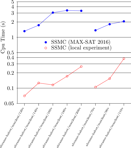
The SSMC contest timings in Figure 3 do not appear consistent with exponential scaling, but a local experiment displays a clear exponential trend of SSMC consistent with our programmed runtimes, Figure 4. Precisely the same codebase and benchmark problems were used. There were slight differences in hardware and compiler, locally LLVM 7.3.0 on an Intel Xeon 2.6GHz Mac Pro, while the contest utilized GCC 4.4.7 on an Intel Xeon 2.0GHz CentosOS Linux server. This seems unlikely to be the cause for this discrepancy in behavior, as borialis also exhibited contest timings very different than those reported in [32].
We believe that whatever factor of the contest environment distorted the runtimes of SSMC consistently affected the other algorithms. Consequently, although we can conclude that SSMC is a competitive solver for the MAX-SAT evaluation, we cannot confidently extrapolate scaling from the contest results from which to compare SSMC with other solvers. In particular, Figure 3 shows a negative slope between the and variable instances (respectively abrame-habet/max2sat/180v and abrame-habet/max2sat/200v). With the programmed runtimes, this is highly unexpected and could not be locally reproduced, but was consistent with the competition results for other solvers. In future work, in order to clarify relative scaling behavior and improve the optimization of SSMC, we plan run several of the solvers submitted to the MAX-SAT competition against SSMC in a local environment that captures timings whose interpretation is more clear.
Acknowledgments: We thank Aaron Ostrander for useful discussions and Yi-Kai Liu for making us aware of [30]. MJ thanks Booz Allen Hamilton for support. Portions of this paper are a contribution of NIST, an agency of the US government, and are not subject to US copyright.
Appendix A Calculations for Example 0
We can re-express (7) as
| (22) | |||||
| (23) |
where
| (24) |
From (23) one can see that the eigenvalue gap of is
| (25) |
Furthermore, the ground state of
| (26) |
is
| (27) |
So, the ground state of is with given by (24). We choose so that at we have . By (24) this entails
| (28) |
With this choice of we have
| (29) |
which is asymptotically a constant, specifically converging to as .
Now, consider the probability distribution sampled by the diffusion Monte Carlo algorithm.
| (30) |
where is the Hamming weight if and
| (31) | |||||
| (32) | |||||
| (33) |
At , and . So, for large
| (34) | |||||
| (35) | |||||
| (36) |
Thus,
| (37) |
at large .
Appendix B Eigenvalue Gap Lower Bound for Example 1
Let be the eigenvalue gap of as defined in (13). In this appendix we prove that occurs at . Note as , the eigenvalue gap of can be obtained by substituting (9) into (25) and expanding to lowest order in , which yields
| (38) |
To prove that occurs at , we introduce the following lemma, which is physically intuitive, and can be regarded as loosely analogous to Le Chatelier’s principle.
Lemma 1.
Let for any two Hermitian operators and . Let be the ground state of , with energy , which we assume to be nondegenerate. For any operator let . Then for all . Also, for all .
Proof.
By the variational principle,
| (39) |
for any . Expanding this yields
| (40) |
By the Hellman-Feynman theorem
| (41) |
Thus the righthand side of (40) is identifiable as the tangent line to at . The fact that lies below its tangent line at every point implies
| (42) |
Taking a derivative of (41) yields
| (43) |
| (44) |
∎
From (10), we find that the ground state of , which is the ground state of satisfies
| (45) |
By Lemma 1, the amplitude in the all zeros state will monotonically increase as is increased beyond . Thus,
| (46) |
With (46) in hand, are now prepared to prove that the eigenvalue gap of monotonically increases for .
Let denote the first excited state of . By the Hellman-Feynman theorem
| (47) |
Substituting in the expression for for , given by (13), (16), and (16) yields
| (48) |
By (46), for all . By the orthogonality of and , this implies for all . Consequently, (48) yields
| (49) |
and therefore the minimum gap in this stage of the adiabatic process occurs at and is as given in (38). (Note that gap at is , and this is the minimum gap for the whole adiabatic process.)
Appendix C Permutation Symmetry and Efficient Spectrum Calculation
In this appendix, we prove that the eigenvalue gap of the matrix is equal to the eigenvalue gap of the block of that acts on the permutation-symmetric subspace. Consequently, we can numerically calculate both the eigenvalue gap of and the ground state eigenvector in time. For example, the data for Figure 2, which extends up to was computed in under an hour on a standard workstation. More generally, for permutation-symmetric Hamiltonians on qubits, the degeneracies ensure that there are only distinct eigenvalues. All of these can be computed in time using the methods outlined in the supplemental material of [14].
Proposition 1.
Let be a Hamiltonian of the form
| (50) |
where . Then the eigenvalue gap of is the eigenvalue gap of the block of acting on the permutation-symmetric subspace.
Proof.
The ground state of is where is the ground state of . Similarly, the first excited level of is -fold degenerate and spanned by
| (51) |
where is the excited state of . Thus, one sees that the ground state of is invariant under all permutations of the qubits and the first excited eigenspace contains a permutation-symmetric state, namely .
Now, recall some standard facts about the spin angular-momentum operators.
| (52) |
The eigenvalues of are for if is even and if is odd. commutes with and therefore they can be simultaneously diagonalized. In the space with eigenvalue (called the spin- space) the eigenvalues of are . The spin- subspace is precisely the permutation-symmetric subspace.
Examining one sees that this means the spin- space has support only on bitstrings with Hamming weights . commutes with . Thus, in an appropriate basis, is block diagonal one block corresponding to each allowed value of .
| (53) |
Now imagine we start with and then increase . The blocks of will be completely unaffected since they act on subspace that exclude Hamming weight zero. Only the block can be affected. The eigenvalues of the operator are and . Thus, by Weyl’s inequality, adding this operator to the block will lower each of its eigenvalues by some amounts between zero and . The ground energy of comes from the block, and the first excited energy degenerately comes from the block. As we increase away from zero, the eigenvalues from this block decrease (or remain constant), while the eigenvalues form the other blocks are unchanged. Thus, the lowest two eigenvalues of will continue to be the lowest two eigenvalues of the block for all positive . ∎
The fact that is permutation-symmetric can be exploited to numerically compute the ground state and ground energy up to large numbers of qubits. Specifically, let be the uniform superposition over all length- bitstrings of Hamming weight .
| (54) |
Then the ground state can be expressed as
| (55) |
The Hamiltonian can be block-diagonalized with one block corresponding to . In particular, a brief calculation yields
| (56) |
Using this formula, one can easily write down an expression for the Hamming-symmetric block of , which is a simple tri-diagonal matrix. Diagonalizing this matrix yields the ground state eigenvalue and eigenvector, as well as the rest of the permutation-symmetric part of the spectrum. From the ground state eigenvector, we can calculate .
References
- [1] Dorit Aharonov, Wim van Dam, Julia Kempe, Zeph Landau, Seth Lloyd, and Oded Regev. Adiabatic quantum computation is equivalent to standard quantum computation. SIAM Journal on Computing, 37(1):166–194, 2007. arXiv:quant-ph/0405098.
- [2] Sergey Bravyi, David P. DiVincenzo, Roberto Oliveira, and Barbara M. Terhal. The complexity of stoquastic local Hamiltonian problems. Quantum Information and Computation, 8(5):361–385, 2008. arXiv:quant-ph/0606140.
- [3] Sergey Bravyi and Barbara Terhal. Complexity of stoquastic frustration-free Hamiltonians. SIAM Journal on Computing, 39(4):1462, 2009. arXiv:0806.1746.
- [4] M. B. Hastings. Obstructions to classically simulating the quantum adiabatic algorithm. Quantum Information and Computation, 13(11/12):1038–1076, 2013. With appendix by M. H. Freedman.
- [5] http://brad-lackey.github.io/substochastic-sat/.
- [6] Edward Farhi, Jeffrey Goldstone, Sam Gutmann, Joshua Lapan, Andrew Lundgren, and Daniel Preda. A quantum adiabatic evolution algorithm applied to random instances of an NP-complete problem. Science, 292(5516):472–475, 2001. arXiv:quant-ph/0104129.
- [7] A. B. Finnila, M. A. Gomez, C. Sebenik, C. Stenson, and J. D. Doll. Quantum annealing: a new method for minimizing multidimensional functions. Chemical Physics Letters, 219:343–348, 1994.
- [8] Sabine Jansen, Mary-Beth Ruskai, and Ruedi Seiler. Bounds for the adiabatic approximation with applications to quantum computation. Journal of Mathematical Physics, 48:102111, 2007. arXiv:quant-ph/0603175.
- [9] Alexander Elgart and George A. Hagedorn. A note on the switching adiabatic theorem. Journal of Mathematical Physics, 53:102202, 2012.
- [10] Edward Farhi, Jeffrey Goldstone, and Sam Gutmann. Quantum adiabatic evolution algorithms versus simulated annealing. arXiv:quant-ph/0201031, 2002.
- [11] Michael Jarret and Stephen P. Jordan. Adiabatic optimization without local minima. Quantum Information and Computation, 15(3/4):0181–0199, 2015. arXiv:1405.7552.
- [12] Vasil S. Denchev, Sergio Boixo, Sergei V. Isakov, Nan Ding, Ryan Babbush, Vadim Smelyanskiy, John Martinis, and Hartmut Neven. What is the computational value of finite range tunneling? Physical Review X, 6:031015, 2016. arXiv:1512.02206.
- [13] Zhang Jiang, Vadim N. Smelyanskiy, Sergei V. Isakov, Sergio Boixo, Guglielmo Mazzola, Matthias Troyer, and Hartmut Neven. Scaling analysis and instantons for thermally-assisted tunneling and Quantum Monte Carlo simulations. arXiv:1603.01293, 2016.
- [14] Sergei V. Isakov, Guglielmo Mazzola, Vadim N. Smelyanskiy, Zhang Jiang, Sergio Boixo, Hartmut Neven, and Matthias Troyer. Understanding quantum tunneling through Quantum Monte Carlo simulations. arXiv:1510.08057, 2015.
- [15] Ben Reichardt. The quantum adiabatic optimization algorithm and local minima. In Proceedings of STOC ’04, pages 502–510, 2004.
- [16] Wim van Dam, Michele Mosca, and Umesh Vazirani. How powerful is adiabatic quantum computation? In Proceedings of FOCS ’01, pages 279–287, 2001. arXiv:quant-ph/0206003.
- [17] Wim van Dam and Umesh Vazirani. Limits of quantum adiabatic optimization. www.cs.berkeley.edu/~vazirani/pubs/qao.pdf, 2003.
- [18] M. H. S. Amin. Effect of local minima on adiabatic quantum optimization. Physical Review Letters, 100:130503, 2008. arXiv:0709.0528.
- [19] M. H. S. Amin and V. Choi. First order quantum phase transition in adiabatic quantum computation. Physical Review A, 80:062326, 2009. arXiv:0904.1387.
- [20] Sergio Boixo, Vadim N. Smelyanskiy, Alireza Shabani, Sergei V. Isakov, Mark Dykman, Vasil S. Denchev, Mohammad H. Amin, Anatoly Yu Smirnov, Masoud Mohseni, and Hartmut Neven. Computational multiqubit tunnelling in programmable quantum annealers. Nature Communications, 7:10327, 2016.
- [21] Lucas T. Brady and Wim van Dam. Quantum Monte Carlo simulations of tunneling in quantum adiabatic optimization. Physical Review A, 93:032304, 2016. arXiv:1509.02562.
- [22] Elizabeth Crosson and Aram W. Harrow. Simulated quantum annealing can be exponentially faster than classical simulated annealing. arXiv:1601.03030, 2016.
- [23] Boris Altshuler, Hari Krovi, and Jérémie Roland. Anderson localization makes adiabatic quantum optimization fail. Proceedings of the National Academy of Sciences, 107(28):12446–12450, 2010.
- [24] Edward Farhi, Jeffrey Goldstone, David Gosset, Sam Gutmann, Harvey B. Meyer, and Peter Shor. Quantum adiabatic algorithms, small gaps, and different paths. Quantum Information and Computation, 11:181–214, 2011. arXiv:0909.4766.
- [25] James King, Sheir Yarkoni, Mayssam M. Nevisi, Jeremy P. Hilton, and Catherine C. McGeoch. Benchmarking a quantum annealing processor with the time-to-target metric. arXiv:1508.05087, 2015.
- [26] M. W. Johnson, M. H. S. Amin, S. Gildert, T. Lanting, F. Hamze, N. Dickson, R. Harris, A. J. Berkley, J. Johansson, P. Bunyk, E. M. Chapple, C. Enderud, J. P. Hilton, K. Karimi, E. Ladizinsky, N. Ladizinsky, T. Oh, I. Perminov, C. Rich, M. C. Thom, E. Tolkacheva, C. J. S. Truncik, S. Uchaikin, J. Wang, B. Wilson, and G. Rose. Quantum annealing with manufactured spins. Nature, 473:194–198, 2011.
- [27] Elizabeth Crosson, Edward Farhi, Cedric Yen-Yu Lin, Han-Hsuan Lin, and Peter Shor. Different strategies for optimization using the quantum adiabatic algorithm. arXiv:1401.7320, 2014.
- [28] Edward Farhi, Jeffrey Goldstone, and Sam Gutmann. Quantum adiabatic evolution algorithms with different paths. arXiv:quant-ph/0208135, 2002.
- [29] R. Grimm and R. G. Storer. A new method for the numerical solution of the Schrödinger equation. Journal of Computational Physics, 4(2):230–249, 1969.
- [30] David Aldous and Umesh Vazirani. “Go with the winners” algorithms. In Proceedings of the 35th Annual Symposium on Foundations of Computer Science (FOCS), pages 492–501. IEEE, 1994.
- [31] Max-SAT 2016, Eleventh Max-SAT Evaluation. http://maxsat.ia.udl.cat.
- [32] Zheng Zhu, Chao Fang, and Helmut G Katzgraber. Borealis–A generalized global update algorithm for Boolean optimization problems. arXiv:1605.09399, 2016.