Compiling Stateful Network Properties
for Runtime Verification

Abstract

Networks are difficult to configure correctly, and tricky to debug. These problems are accentuated by temporal and stateful behavior. Static verification, while useful, is ineffectual for detecting behavioral deviations induced by hardware faults, security failures, and so on, so dynamic property monitoring is also valuable. Unfortunately, existing monitoring and runtime verification for networks largely focuses on properties about individual packets (such as connectivity) or requires a digest of all network events be sent to a server, incurring enormous cost.

We present a network monitoring system that avoids these problems. Because traces of network events correspond well to temporal logic, we use a subset of Metric First-Order Temporal Logic as the query language. These queries are compiled down to execute completely on the network switches. This vastly reduces network load, improves the precision of queries, and decreases detection latency. We show the practical feasibility of our work by extending a widely-used software switch and deploying it on networks. Our work also suggests improvements to network instruction sets to better support temporal monitoring.

1 Introduction

Network configurations are challenging to get right, and can be difficult [30, 39] to debug. Not only do they dictate static forwarding and packet-filtering behavior, they also control dynamic, stateful features such as shortest-path routing, network-address translation, caching for various protocols, and more. Given the ubiquity and criticality of networks, operators must be able to develop confidence in their configuration.

The difficulty is compounded in Software Defined Networks (SDNs), where operators can write their own controller programs to govern switch behavior. Not only is network behavior now defined by programs rather than configurations (which tend to be of limited expressive power and thus more amenable to reasoning [2, 11, 14, 20, 22, 29]), but the mechanics of SDN itself induce new types of bugs [18, 32] that must be addressed.

Static network-property checking tools like VeriFlow [15] and NetPlumber [14] are powerful, but limited in scope to to stateless forwarding policies. Static tools designed specifically for SDNs will also function weakly at best in a hybrid network that uses both SDN and traditional elements. Factors like mis-connected cables [13], external attacks, and complex hardware problems [18] further demonstrate that static tools are complementary to and must be supported by strong runtime checks.

Purpose-built middleboxes, such as intrusion-detection systems, monitor and react to traffic efficiently—often at line rate or close to it. But these are costly, lack general-purpose flexibility, and sit at least one step removed from the forwarding performed by the switches. High-performance Network Function Virtualization (NFV) solutions (e.g. [23, 31]) are now able to process traffic at or near line rate (10Gpbs), but still require traffic to be rerouted through them. Another class of monitoring tools, including NetSight [12] and Simon [28], send digests of packets seen to a central server—an approach that adds flexibility while incurring significant cost.

Narayana, et al. [26] introduce a different technique: compiling regular-expression path queries down to rules executed by switches. However, path queries are limited to expressing how a single packet traverses the network, independent of history. History is vital for monitoring the stateful behavior of protocols and applications. A central server might support stateful queries by updating stateless rules on each switch as needed, but this approach increases latency, server load, and risk that the monitor will be impacted by reordering, retransmission, or other eccentricities of the network.

Instead, we present Varanus, a novel system for stateful runtime verification of network-control programs: compiling temporal queries in their entirety to the switches themselves. Our switch-centric capture approach has several key advantages. It:

• reduces load on the controller and/or monitoring server;

• decreases latency of detection and state-transition, which also lessens the potential for unsound results (Sec. 7.0.1);

• avoids potential event re-ordering induced by transmission to a central server; and

• increases the expressive power of queries by exposing how the switch transforms an arriving packet into a departing packet, without resorting to unsound methods such as comparing payload-hashes [12].

This approach is challenging because switches are optimized to match and forward packets as quickly as possible, limiting the expressive power of rules they can execute. In fact, current standard switch-rule formats are entirely stateless, making temporal-query compilation unworkable. Nevertheless, switches do have non-trivial computational resources: a slower, more expressive tier of processing sits above its fast, limited matching capabilities in order to handle rule-updates from the controller and other operations that cannot be performed at line rate. Varanus takes advantage of this, conservatively extending switch rules to support a constrained subset of Metric Temporal Logic, retaining fast match capabilities at the lower tier while performing state updates in the higher tier—balancing expressiveness with performance. We demonstrate feasibility by modifying a popular software switch and deploying queries in a network.

2 Queries: Examples, Syntax, Semantics, and Expressive Power

Before detailing Varanus’s query syntax and semantics, we first motivate temporal queries with a small example: monitoring a stateful-firewall SDN application.

2.1 Queries by Example

A stateful firewall blocks packets that arrive on external ports unless they are part of a connection initiated from the internal network. Compared to most network applications, a stateful firewall is relatively simple, yet its implementation could contain many bugs: outgoing traffic or valid incoming traffic could be rejected (resulting in a connectivity failure), or invalid external traffic could be permitted (a security threat). For simplicity, we limit the firewall switch to two ports: internal and external. We also introduce a black-listed external host with network address 192.0.2.1. We now have a number of correctness properties; for instance:

1. Packets from host 192.0.2.1 never egress the firewall.

2. Packets arriving at an internal port are always forwarded to the external port.

3. After a packet from internal host A to external host B arrives at an internal port, packets from B to A arriving at an external port will be output on the internal port for the next ten seconds.

4. If no packet from internal host A to external host B has previous arrived at an internal port, packets from B to A at an external port will be dropped.

We wish to monitor the network for counterexamples, i.e., traces of network events that falsify each property.

Property 1

If the switch never modifies the IP source field, then this property can be monitored by a single stateless packet filter that checks for blacklisted packets departing from the firewall. The corresponding query is:

⬇

1see p: egress | p.nwSrc = 192.0.2.1

which notifies the monitor when the switch observes a packet egress with source network address 192.0.2.1—either to raise an alert or to trigger further processing.

Property 2

In contrast to the prior property, this one requires state: the system only incurs an obligation to forward a packet once it has arrived. Detecting when this property fails means looking for cases when a packet egresses in an unexpected way (e.g., it is dropped). Thus, we now have a sequence of two observations:

⬇

1see p: arrival | p.locPt = 1 // Internal port

2see p’: egress same | p’.locPt != 2 // External port

These lines should be read with an implicit “followed by” between them. The identifier p matches an arbitrary packet arrival at the internal port (1). Next, p’ matches when the packet is not seen departing the external port (2). The same annotation specifies that p’ must be an egress for the packet identified in the previous arrival observation (p). The second observation depends on the first; a given egress only discharges the obligation incurred by its preceding arrival.

Property 3

The obligation in this property is only incurred after multiple distinct packets:

⬇

1see p1: arrival | p1.locPt = 1

2see p2: arrival within 10 | p2.locPt = 2, p2.nwSrc = p1.nwDst,

3 p2.nwDst = p1.nwSrc

4see p2’: egress same | p2’.locPt != 1

The identifier p1 matches a packet arriving at the internal port, which should open a hole in the firewall for return traffic. p2 is a corresponding return packet arriving on the external port within 10 seconds of p1. The observation for p2’ matches when p2 does not depart on port 1, meaning it was not forwarded to the internal network.

Property 4

Here, a counterexample must contain no analogue to p1 in the above:

⬇

1not see p1 | p1.locPt = 1, p2.nwSrc = p1.nwDst, p2.nwDst = p1.nwSrc

2 until see p2: arrival | p2.locPt = 2

3see p2’: egress same | p2’.locPt = 1

The first observation (lines 1–2) matches an incoming packet p2 on the external port, provided that no packet p1 (bearing reversed addresses) has previously arrived at the internal port. p2’ then observes that p2 has erroneously been forwarded.

Even these short examples require non-trivial features: recognizing chains of related observations, time-dependence, detecting when two events involve the same packet, negative observations, awareness of prior events, etc.

2.2 Syntax

A query comprises an ordered list of observations $[O_{1},...,O_{n}]$, each of which matches a network event (a positive observation) or lack of an event within some period of time (a negative observation). Each observation has a type: either a packet arrival or packet egress (possibly with temporal constraints).

Each observation also contains a trigger event identifier and a match predicate which references that identifier and (optionally) identifiers of prior positive observations. Also, until observations contain a blocking event identifier and a corresponding blocking predicate. Each predicate consists of a set of literals. Fig. 1 gives the complete grammar.

⬇

QUERY ::= LISTOF(OBSERVATION)

OBSERVATION ::=

"see" ID ":" TYPE "|" PREDICATE |

"not see" ID ":" TYPE "|" PREDICATE |

"not see" ID "|" PREDICATE

"until" see ID ":" TYPE "|" PREDICATE |

PREDICATE ::= LISTOF(ATOMIC)

ATOMIC ::= TERM "=" TERM | TERM "!=" TERM

TERM ::= NUM | ID.FIELD

TYPE ::= "arrival" | "arrival within" NUM |

"egress" | "egress within" NUM | "egress same"

FIELD ::= dlTyp | dlSrc | dlDst | nwSrc | nwDst | nwProto | ...

Figure 1: Query syntax. Non-terminals are capitalized, and LISTOF(X) denotes a list of expressions matching non-terminal X. FIELD matches any valid packet field name.

 

To be well-formed, a query $[O_{1},...,O_{n}]$ must also satisfy the following:

• every negative observation has a within annotation;

• the same type annotation only occurs with egress;

• every egress same observation is preceded by a positive arrival observation;

• each $O_{i}$, $O_{j}$ ($i\neq j$) are labeled by different identifiers; and

• each $O_{i}$’s predicate refers only to its own identifier and (optionally) identifiers of prior observations $O_{j}$ ($j\leq i$).

These ensure key semantic requirements, e.g., every term is bound before it is used.

2.3 Semantics

Queries match traces of events in the network. Observations within a query match individual events or timeouts in the context of a trace. To make this precise, we first introduce some notation.

An event is one of: a packet arrival, a packet egress, a clock tick (written as $\mathit{TICK}$), or the no-op event ($\bot$) which the semantics uses as a placeholder when no event has yet occurred. A timestamp is a non-negative integer value. A trace is a finite sequence of $($event, timestamp$)$ pairs with monotonically non-decreasing timestamps. For a trace $T$, we use $\pi_{i}(T)$ to refer to the $i^{th}$ event in a trace and $\tau_{i}(T)$ to refer to its timestamp. $\text{suffix}_{k}(T)$ denotes the suffix of $T$ obtained by removing the leading $k$ elements. We omit the application “$(T)$” where the trace is clear from context.

Each query has a fixed set of query terms $R$: the e.fld expressions that occur within its observations. Since there are finitely many observations in a query, and only finitely many valid field names, the set of query terms is always finite. To project out individual field values from events, we use a partial function $getf:Events\times FIELD\rightarrow NUM$. If an event $e$ does not contain a field f, then $getf(e,f)$ is undefined. We use $O(e)$ to indicate an observation whose match identifier is $e$; for an until observation, this is the identifier in the second position, i.e., the trigger. We assume traces contain a discrete tick event for each positive integer $i$, denoted $(\mathit{TICK},i)$; this is for convenience in the formalism for observations using within, which in practice (Sec. 5) will be implemented via switch-rule timeouts.

For every query $Q$ and trace $T$, we now define whether $T$ satisfies $Q$ (written as $T\models Q$). Since $Q$ is a sequence of observations $[O_{1},...,O_{n}]$, we must also define whether $T$ satisfies each observation $O_{i}$. But whether $T\models O_{i}\,(1\leq i\leq n)$ may depend on when and how previous observations were satisfied: $O_{i}$ may reference field values bound by $O_{1},...,O_{i-1}$, and may also, via within keyword, depend on the time since the last observation was satisfied. We provide this past-time context via an environment $\eta$, which maps syntactic query terms to concrete values such as packet fields. For instance, $\eta$ may map p1.nwDst (the network destination address of the event bound to p1) to 10.0.0.1.

Fig. 2 defines the meaning of a query via a logical satisfaction ($\models$) relation, similarly to temporal logic. Since this semantics introduces numerous parameters, for brevity we write $T\models Q$ for $T\models_{\emptyset,0,\bot}Q$, omitting the initial environment, last-match timestamp, and last-match event.

Atomic Formulas ($\mathbf{m}$) and Predicates (C) match an event with respect to an environment.
$\pi\models_{\eta}\text{\tt e.f = c}$	$\iff$	$getf(\pi,f)=c$
$\pi\models_{\eta}\text{\tt e.f1 = e.f2}$	$\iff$	$getf(\pi,f1)=getf(\pi,f2)$
$\pi\models_{\eta}\text{\tt e.f1 = t}$	$\iff$	$getf(\pi,f1)=\eta(t)$
(if t a term that is neither c nor e.f2)
$\pi\models_{\eta}\text{\tt t1 != t2}$	$\iff$	$\pi\not\models_{\eta}\text{\tt t1 = t2}$
$\pi\models_{\eta}\mathtt{m_{1},...,m_{k}}$	$\iff$	$\forall m_{i}.\pi\models_{\eta}m_{i}$

Event Types ($\mathbf{Y}$) match a trace position with respect to an environment,
a last-match timestamp, a last-match event, and an operator ($\leq$ or $=$).
$T,i\models_{\eta,l_{\tau},l_{\pi},op}\text{\tt arrival}$	$\iff$	$\pi_{i}$ is a packet arrival
$T,i\models_{\eta,l_{\tau},l_{\pi},op}\text{\tt egress}$	$\iff$	$\pi_{i}$ is a packet egress
$T,i\models_{\eta,l_{\tau},l_{\pi},op}\text{\tt arrival within D}$	$\iff$	$\pi_{i}$ is a packet arrival, and $\tau_{i}\,op\,(l_{\tau}+D)$
$T,i\models_{\eta,l_{\tau},l_{\pi},op}\text{\tt egress within D}$	$\iff$	$\pi_{i}$ is a packet egress, and $\tau_{i}\,op\,(l_{\tau}+D)$
$T,i\models_{\eta,l_{\tau},l_{\pi},op}\text{\tt egress same}$	$\iff$	$\pi_{i}$ is a packet egress, and $I(l_{\pi},\pi_{i})$

Observations ($\mathbf{O}$) match a trace position with respect to an environment,
a last-match timestamp, and a last-match event.
$T,i\models_{\eta,l_{\tau},l_{\pi}}$	see e : Y | C	$\iff$	$T,i\models_{\eta,l_{\tau},l_{\pi},\leq}Y$ and $\pi_{i}\models_{\eta}C$
$T,i\models_{\eta,l_{\tau},l_{\pi}}$	not see e : Y | C	$\iff$	$T,i\models_{\eta,l_{\tau},l_{\pi},=}Y$, $\pi_{i}=\mathit{TICK},\text{ and }$
			$\forall j(0\leq j<i),\pi_{j}\not\models_{\eta}C$
$T,i\models_{\eta,l_{\tau},l_{\pi}}$	not see e1 | C1		$T,i\models_{\eta,l_{\tau},l_{\pi},\leq}Y$, $\pi_{i}\models_{\eta}C2\text{ and }$
	until see e2 : Y | C2	$\iff$	$\forall j(0\leq j<i)$, either
			$T,j\not\models_{\eta,l_{\tau},l_{\pi},\leq}Y$ or $\pi_{j}\not\models_{\eta+[e2,\pi_{j}]}C1$

Queries ($\mathbf{Q}$) match traces with respect to an environment, a last timestamp, and a last event.
$T\models_{\eta,l_{\tau},l_{\pi}}\mathtt{O_{1}(\mathtt{e_{1}}),...,O_{n}}$	$\iff$	$\exists i\geq 0\,|\,T,i\models_{\eta,l_{\tau},l_{\pi}}\mathtt{O_{1}},\text{ and }$
		$\text{suffix}_{i+1}\models_{\eta+[e_{1},\pi_{i}],\tau_{i},\pi_{i}}\mathtt{O_{2},...,O_{n}}$

Figure 2: Logical Semantics for Queries, Observations, event types, predicates and atomic formulas. We use $\eta+[e,\pi]$ as shorthand for $\eta[\forall f\in\mathtt{FIELD},\;\mathtt{e.fld}\mapsto getf(\pi_{i},f)]$, i.e., environment $\eta$ extended by the fields of $\pi$ under identifier e. The symmetric binary relation on events, $I$, represents whether two events involve the same packet.

 

2.4 Expressive Power

Since Varanus’s language can match sequences of events, it has a clear expressive advantage over existing work that focuses only on stateless monitoring. Implementations of real world protocols, such as ARP and DHCP, as well as bespoke SDN controller programs require a stateful monitoring language. While more expressive monitoring solutions exist, such as Simon [28], these approaches are not conducive to switch-based state management. (Sec. 6 discusses other work in more detail.) Our language provides a novel middle-ground: meeting the expressive demands of stateful monitoring while also achieving the benefits of switch-based capture.

Comparison to Temporal Logic

Our query language comprises a strict subset of Metric First-Order Temporal Logic (MFOTL) [4] that is conducive to execution on switches. In essence, positive observations correspond to $F$ (“finally”) or $U$ (“until”) formulas, and negative observations to $G$ (“globally”) formulas, with later observations nesting. Forward references in until observations can be expressed in MFOTL using existential variables. For instance, not see e1 | e1.nwSrc = e2.nwDst until see e2: arrival corresponds to $\exists x.\,\neg(src=x)\,U_{[0,\inf)}\,(dst=x)$. The fixed temporal structure of queries—observation followed by observation—leads to restricted formula nesting in the equivalent MFOTL, easing compilation while sacrificing expressive power. For example, there is no equivalent query for the MFOTL formula $F\alpha\wedge F\beta$. Also, while the within keyword allows observations to be satisfied at any point within the interval $[0,D]$, MFOTL allows both ends of intervals to be specified. This limitation makes it possible to compile within via switch rule timeouts (Sec. 4).

Additional Examples

To demonstrate the broad applicability of this technique, Fig. 3 lists additional stateful properties for five example applications not seen in Sec. 2.1: (1) a learning switch, which learns how to reach new destinations as it observes traffic; (2) a Network Address Translation (NAT) application, which masquerades multiple hosts as a single address; (3) an Address Resolution Protocol cache, which facilitates fast lookup between layer 2 and layer 3 addresses; (4) a packet-tagging application; and (5) port knocking, which allows traffic from external hosts that send a pre-specified packet sequence. Each of these safety properties can be expressed as a query in Varanus.

App	Property	N?	IE?	U?
Learning	Never flood after destination learned
Switch	Once destination learned, send out correct port
NAT	NAT ports used consistently once assigned		✓
ARP	No new requests generated for cached addresses
Cache	Requests for cached addresses always replied to	✓
	If no prior request received, propagated on core ports	✓		✓
VLAN	Once a tag is seen on a port, never see another
and misc.	See at most $k$ distinct tags on any port
tagging	Untagged packets always tagged before departure on trunk		✓
	Tagged packets always de-tagged before departure on access port
Port Knocking	Recognize correct knocking sequence			✓
	Knocking packets should be dropped		✓

Figure 3: Select additional stateful queries, beyond those in Sec. 2.1, which fit our language. Columns 1 and 2 name the specific program and property. Additional columns contain a ✓ if the query uses negative observations (N?), ingress-egress pairing (IE?), or until observations (U?).

 

3 Queries as Automata

We now show how a query can be realized as a non-deterministic automaton over event traces. This fact will be useful for compilation: in Sec. 4 we will see that each state of these automata can be represented as a set of switch rules.

Intuitively, a state of such an automaton carries several things: (1) which observation was last matched; (2) the current environment; (3) a set of forbidden environments; (4) a last-match event; and (5) a last-match timestamp. Much of this state-construction echoes the semantics in Sec. 2; the only exception is (3), which allows the automaton to remember previously seen events that matched the blocking part of an until observation.

Given a query $Q=[O_{1},...,O_{n}]$, let $H(R)$ be the set of all environments over the query terms $R$ of $Q$ and let $|Q|$ be the set $\{O_{1},...,Q_{n}\}$. The query automaton for $Q$, denoted by $\mathcal{A}_{Q}$, is the non-deterministic automaton $(S,\Sigma,\delta,s_{0},F)$ where:

1. the set of states $S$ is $(|Q|\times H(R)\times 2^{H(R)}\times\mathit{Event}\times\mathbb{N})\cup\{(O_{0},\emptyset,\emptyset,\bot,0)\}$ (where $O_{0}$ is a distinct value representing “no observations satisfied”);

2. $\Sigma$ is a set of possible $($event, timestamp$)$ trace elements;

3. $\delta$ is a relation on $S\times\Sigma\times S$ (the transition relation);

4. $s_{0}=(O_{0},\emptyset,\emptyset,\bot,0)$ is the unique starting state; and

5. the set of accepting states $F=\{(o,\eta,\widehat{\eta},\pi,\tau)|o=O_{n}\}$; i.e., all states for which the final observation has been matched.

$$\delta_{i} =\delta_{i}^{loop}\cup\delta_{i}^{ok}$$

$$\delta_{i}^{loop} =\{((Q_{i},\eta,\widehat{\eta},l_{\pi},l_{\tau}),(\pi,\tau),(Q_{i},\eta,\widehat{\eta},l_{\pi},l_{\tau}))$$

for every $$\eta \widehat{\eta} l_{\pi} l_{\tau} \pi \tau$$, , , , , and

unless $$\pi\models_{\eta}C \pi \tau=l_{\tau}+D$$ or (=TICK and )

$$\delta_{i}^{ok} =\{((Q_{i},\eta,\widehat{\eta},l_{\pi},l_{\tau}),(\pi,\tau),(Q_{i+1},\eta+[e,\pi],\emptyset,\pi,\tau))$$

$$\text{ where }\pi=TICK\text{ and }\tau=l_{\tau}+D\}$$

Figure 4: Producing the non-deterministic transition relation for a query $[O_{1},...,O_{n}]$. The notation $A-[e]$ means the subset of match predicate $A$ with all literals involving event $e$ removed. For space, we show only the not see within case here; Appendix 0.A contains the full table.

 

If $\delta$ is undefined for a particular state and input, the automaton is said to halt on that pair. The automaton accepts a trace if there is some run on the trace that ends in an accepting state. Given a finite-branching transition relation, every finite trace induces only finitely many runs. The transition relation $\delta$ is defined as $\delta=\bigcup_{1\leq i<n}\delta_{i}$, and each $\delta_{i}$ is defined for each observation $O_{i}$. Fig. 4 gives $\delta_{i}$ for one type of observation; Appendix 0.A provides the full definition. The automata produced here are quite limited: the only cycles they contain are self loops, and environments grow monotonically as each run evolves. Furthermore, $\delta$ is finite-branching. The only subtlety is in $\widehat{\eta}$, which represents forbidden bindings accumulated in the course of matching an until observation. Fig. 5 demonstrates a partial run of the automaton for Property 4 of Sec. 2.1. Query automata correspond closely to queries, as the following theorem (proven in Appendix 0.B) shows:

Figure 5: Example run of the automaton for Property 4 (timer details omitted). The starting state has empty $\eta$ and $\widehat{\eta}$ and waits for p2. When a packet (A) matching p1 arrives, the new state continues waiting for p2, but has learned a forbidden environment. Since (B) matches p2 but does not match the forbidden environment, it advances the state to waiting for p2’. If B egresses (not shown) at port 1, the automaton advances to an accepting state.

 

Theorem 3.1

Let $T$ be a trace and $Q=[O_{1},...,O_{n}]$ a query. Then $T\models Q\iff\mathcal{A}_{Q}$ accepts $T$.

The Role of Non-determinism in this Domain

Non-determinism allows multiple runs of $\mathcal{A}_{Q}$ to co-exist. Consider the query:

⬇

1see p1: arrival | p1.nwSrc = 10.1.1.1

2see p2: arrival | p2.nwDst = p1.nwDst\end{lstlisting}

3executed over a trace containing packets with multiple destination addresses. Each destination

4will produce a distinct environment binding \qry{p1.nwDst}, necessitating multiple

5states be ‘‘active’’ at any one time. Timers also make heavy use of non-determinism, even

6for queries where no environment is needed. For instance:

7\begin{lstlisting}[label=lst:need-nd2,language=query]

8see p1: arrival | p1.nwSrc = 10.1.1.1

9see p2: arrival within 5 | p2.nwDst = 10.1.1.2

10see p3: arrival within 5 | p3.nwSrc = p3.nwDst

This query is entirely positive, and requires no environment to evaluate—the constraints on p2 are not dependent on p1. Suppose we execute it on the following event trace:

⬇

t=0: nwSrc = 10.1.1.1, nwDst = 10.1.1.5 [matches p1]

t=4: nwSrc = 10.1.1.1, nwDst = 10.1.1.2 [matches p1,p2]

t=8: nwSrc = 10.1.1.10, nwDst = 10.1.1.2 [matches p2]

t=10: nwSrc = 10.1.1.3, nwDst = 10.1.1.3 [matches p3]

Any individual run will time out after 5 seconds of waiting for p2, but non-deterministic automata can have multiple simultaneous states. This allows the wait for p2 to be extended via a new state at t=4, enabling the capture of p2 at t=8. (The logical semantics enable this via “for some $i$” in the Q portion of Fig. 2.) Rather than attempting to determinize query automata, we will embrace non-determinism and use it explicitly in our compiler.

4 Compilation

Varanus generates switch rules in an extension of OpenFlow [24], a widely-used protocol that allows the controller to install persistent forwarding rules on switches. The OpenFlow protocol is widely supported both by major hardware vendors, and by software switches such as Open vSwitch [33]. Because of this extensive support, our compiler targets OpenFlow, although the approach is not OpenFlow specific.

The OpenFlow standard continues to evolve, and individual vendors also extend the protocol to provide new features. Our work fits into this culture of extension, using monitoring to explore the benefits of carefully increasing the OpenFlow instruction set.

4.1 Background

In OpenFlow, the rules that dictate switch behavior are held in ordered collections called tables. An OpenFlow rule is a tuple $(D,T,M,A)$ consisting of an optional hard timeout duration, a table identifier, a set of match criteria, and a set of actions to perform if the rule is matched. Match criteria are predicates that match packet fields against values, possibly with wildcarding. For instance, a rule might match packets with source IP address 10.1.1.* and destination TCP port 80. Actions include forwarding the packet out a constant port (out(k)), overwriting a packet field with a constant value (fld:=val), resubmitting the packet to a constant table (resubmit(t)), and sending the packet to the controller for further instructions (controller). Rules also contain a numeric priority, which we abstract out and give implicitly via list ordering.

When a packet arrives, it is submitted to table $0$. Within each table, the highest-priority matching rule applies, and its actions are added to the overall action set. The switch performs all actions in the set, in a fixed order (i.e., field modifications before output), once no further table resubmits are mandated. The graph of resubmits must be acyclic. An empty action set results in a dropped packet. If the packet matches no rule in any table, it is sent to the controller. Crucially, this packet-evaluation process leverages the limited expressive power of rules to process packets quickly, whether via specialized data-structures in software or optimized hardware. Only cache-misses and modifications to the rule-set need pass through a switch’s slower general-purpose datapath.

In effect, these simple static rules are a cache of controller instructions, which may be proactively installed. In standard OpenFlow, only the controller, and not the switch itself, can modify or install rules. This provides a clear separation of concerns between switch and controller, but leads to increased latency and load. Different dynamic-rule extensions have been proposed, which we compare in Sec. 6. Open vSwitch also implements a dynamic extension: the “learn” action, which allows a rule, when matched, to install a new rule that does not itself use the learn action. Our own extensions build atop this.

4.2 Rule Extensions with Dynamic Actions

Varanus extends the learn action to allow learned rules to themselves have learn actions, i.e., we enable nesting rules to be learned up to arbitrary bounded depth. Concretely, we extend OpenFlow as follows: an OpenFlow⁺ rule is a tuple $(D,T,M,A,O)$ where $O$ is an action set to perform on rule timeout. Other components are identical to OpenFlow, except that the set of permitted actions in $A$ is larger, including deleting all rules in the current table (delete_all), incrementing an atomic counter (inc(c)), and learning a new rule (learn(r)). Table identifiers are split between ingress and egress tables; egress tables apply immediately before the packet departs (or is dropped by) the switch.

4.3 Compiling to Switches

To realize $\mathcal{A}_{Q}$ as a set of OpenFlow⁺ rules, Varanus produces an initial rule set that embodies the automaton’s starting state. It contains, via nested learn actions, a blueprint for all possible runs of $\mathcal{A}_{Q}$. Since the switch accumulates an action set from all tables before discharging the packet, this gives us a way to implement non-determinism: every table corresponds to an active run of $\mathcal{A}_{Q}$. Separate table spaces for ingress and egress maintain the distinction between arrival and egress events.

Consider a run of $\mathcal{A}_{Q}$ in state $S=(O_{i},\eta,\widehat{\eta},l_{\tau},l_{\pi})$. If $S$ is an accepting state, no rules are required; the monitor will have been notified on transitioning to $S$. If $S$ is not accepting, there are four varieties of transitions to cover: (1) true self-loops (defined by each $\delta^{loop}$ in Fig. 4); (2) halting; (3) forward transitions from an $O_{i}$ state to a $O_{i+1}$ state ($\delta^{ok}$ in Fig. 4); and (4) in the case of until, blocking self-loops that rule out potential forward transitions but remain in a state with the same $O_{i}$ component ($\delta^{block}$ in Appendix 0.A’s Fig. 7). The compiler addresses these as follows:

1. Self-loops are the default; if an event matches no rules, no action is taken.

2. A run halts in two cases: when a timed positive observation times out, or a negative observation is matched. The compiler realizes these by adding a timeout to corresponding rules. For positive observations, the timeout erases the rules; for negative observations, forward-transitions execute on timeout and matching packets delete the rules. Since tables correspond to runs of $\mathcal{A}_{Q}$, deleting a table removes that run.

3. Forward transitions use either the learn action (to learn rules into a fresh table) or the controller action (to notify the monitor that the query has been satisfied).

4. To realize the blocking transitions for until observations, the compiler adds an extra, low-priority rule that, as blocking events are seen, learns new rules to block corresponding packets from triggering forward transitions.

The Varanus compiler recursively descends through each observation, building a corresponding set of switch rules. Where match predicates involve negative literals, the compiler inserts shadow rules before the trigger rule that advances the state. Since only one rule per table can apply, these block the trigger from applying.

Observations in a query can reference previously seen events, but switch rules cannot carry an environment directly. To bridge this gap, we exploit techniques used for compiling the lambda calculus: substitution and De Bruijn indices [9]. The compiler embeds current values via substitution as new rules are learned. To prevent premature substitution, every field reference in switch rules also carries a deferral value. Where De Bruijn indices count how many bindings away a variable was bound, deferral values count the number of learn actions to wait before substituting. Our extensions to OVS read these deferral values when learning, perform substitution if it is zero, and otherwise decrement it in the new learned rule. Appendix 0.C gives the algorithm in full.

5 Implementation and Evaluation

Our implementation comprises the compiler of Sec. 4 and a version of the Open vSwitch [33] software that has been modified to support OpenFlow⁺. We also use a proxy between the switch and any controller applications (such as the stateful firewall in Sec. 2.1), allowing us receive query notifications and place any application-installed rules between our compiled ingress and egress tables. We optimize pairs of ingress/egress same observations by using switch registers to maintain ingress field values as needed; this allows us to avoid queuing packets until all learn actions are complete.

The full version of OpenFlow involves advanced features not mentioned above; we have discarded these for simplicity in our prototype. Consequently, our ability to detect egresses is limited to packets emitted on zero, one, or all ports (i.e., not multicast).

Performance Evaluation

The key performance metric in our approach is the time required to match packets in our query tables, which directly affects forwarding latency. This additional latency includes the time to execute our modified learn actions, and the time to evaluate a packet in each active table. Since the time to execute our modified learn actions does not differ significantly from the time to execute a standard learn action, we focus on the number of active tables. Critically, the number of tables affects all packets processed by Open vSwitch’s tables, not just those that match a query observation. To quantify the latency introduced by adding tables, we created a test network using an installation of Open vSwitch with our extensions and two hosts running in Mininet [19].

OVS maintains a low-level cache of actions for packets already processed by rule tables. In order to focus on the packets most affected by our modifications, we manufacture a worst-case situation by creating a large number of fresh TCP connections, which result in cache misses, each of which causes all tables to be evaluated. We measured the latency of rules that allocate a new table for each new TCP connection entering the switch, similar to the stateful-firewall queries of Sec. 2.1. We generated traffic using ovs-benchmark [33], a performance measurement tool included with Open vSwitch, and captured traffic with the tshark packet-analysis tool. We examined the round trip time for the first two packets in the TCP handshake, which is the portion of the connection that must be processed by the slow path. To understand how the latency changes based on the number of active runs of the automaton, we varied the numbers of new connections per second and the duration of the timeout on installed rules. (Without timeouts, the amount of query state retained increases monotonically as packets are processed, which becomes intractable.) For each set of parameters, we conducted measurements for 5 minutes of constant traffic at the specified rate, which we express as a CDF in Fig. 6.

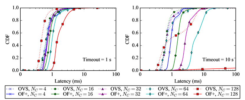
Figure 6: CDF of latency for a base installation of Open vSwitch (OVS) and our modified switch with support for OpenFlow⁺ rules (OF+). Our evaluation measured the latency to process a new connection for a number of new connections per second ($N_{C}$) and with rule timeouts of 1 second (left) and 10 seconds (right), shown on a log scale. Evaluating OpenFlow⁺ rules at 128 connections/sec with 10 second timeouts (not fully pictured) shows prohibitively high latencies in the 1-10sec range.

 

To provide a baseline for the performance of the learn action, we use an unmodified OVS installation learning new rules into a single table for each new TCP connection seen. In unmodified OVS, the learn action has a latency of about 1 millisecond, due to the need to perform an expensive rule table update for each packet. This latency increases based on the number of new connections and rules in the table, as shown in Fig. 6.

The difference between the baseline implementation and Varanus is reflected in Fig. 6 as the horizontal distance between OVS (dashed lines) and OpenFlow⁺ (solid lines), and is due to the added cost of maintaining and evaluating multiple OpenFlow⁺ tables. In our test network, traffic at 64 new connections per second with 1 second rule timeouts can be handled by about 500 tables (one for each of the 8 packets in each ovs-benchmark TCP connection within the one-second window) and incurs a latency under 1 ms. 128 new connections per second, requiring 1000 tables, are each handled within 10ms. For the 10 second timeout case, the latencies are much higher due to the increased number of active tables; at 128 connections per second with 10 second timeouts, we reach the resource limit of our test switch at approximately 8000 tables, which presents as an unacceptably high latency (on the order of tens of seconds), since uncached table evaluation cannot keep up with the new traffic.

These measurements indicate that Varanus can be practical on a small network; we allow the user to select suitable timeout values for their queries, as they are in the best position to know both their needs and what their environment can support. Sec. 7 discusses future work on alternative approaches that improve scaling on larger networks.

6 Related Work

Metric temporal logics have been used previously for runtime verification, notably by Basin, et al. [4], whose MonPoly tool monitors a richer subset of MFOTL formulas—including unrestricted nesting and two-sided intervals—than our approach. Kim, et al. [17] also give a runtime program monitoring framework, MaC, with a query language inspired by past-time LTL with intervals. Their language adds state via “auxiliary variables”, which are updated as a monitoring script progresses through an event stream. MaC’s support for time intervals and aggregation is superior to ours, but as auxiliary variables are limited to basic Java types (e.g., numbers), the language cannot support branching caused by non-deterministic interleaving (Sec. 3). The Eagle [3] monitoring logic is also more expressive than ours, allowing the definition of new temporal operators. Deshmukh, et al. [10] perform off-line system monitoring using Signal Temporal Logic, which enables checking quantitative, rather than strictly Boolean, properties. All these works assume a standard Turing-complete execution target. In contrast, Varanus integrates with existing switch software to minimize the impact of on-line capture and stateful filtering. General monitoring tools also neglect network-domain distinctions such as the connection between packet ingress and corresponding egress.

Simon [28] provides a scriptable, interactive monitoring framework for SDN programs. However, Simon runs on a centralized server, which means all packet events on the network must be communicated to this server, whereas our approach reduces load and improves event granularity. Events generated by Varanus could be provided to Simon streams for further processing and interactive exploration.

Narayana, et al. [26] compile “path queries” about packet forwarding to switches. Path queries, by their nature, are distributed across multiple switches, whereas we compile stateful queries only for single switches. Path queries are restricted to regular expressions over possible forwarding paths, and so cannot express the array of stateful properties that Varanus targets, but do not require extensions to OpenFlow.

DMaC [41] extends MaC to networking by compiling MaC properties to Network Datalog [21]. DMaC can describe both stateful and path-specific properties, and can monitor behavior across multiple switches, whereas our properties are single-switch. DMaC requires that switch state and traffic information be made available in a form it can query, and executes via a custom Datalog engine on software switches. Since our goal is to filter for temporal packet sequences on optimized switch software—with minimal impact on forwarding speed—our switch-rule based approach differs significantly.

NetSight [12] captures packet trajectories by capturing digests for each packet, which are processed off-switch. As our work focuses on compiling temporal, multi-packet queries to switches, it is largely orthogonal, but our extensions to switch rules potentially provide NetSight with a means to reduce the number of packet digests produced. Moreover, NetSight differentiates packets by hashing, whereas our approach allows a more fine-grained distinction.

Production SDN monitoring fabrics, such as BigTap [7], are limited to operations supported by current versions of OpenFlow, and thus cannot avail themselves of switch-side stateful monitoring. Planck [35] and other sampling approaches deliberately compromise on completeness in the face of intrinsic network constraints. We do not sample deliberately, although overfull switch queues can manifest similarly (Sec. 7.0.1).

Numerous other tools (e.g., [34, 1, 42]) perform runtime monitoring, but either lack compilation to switches or monitor only single-packet paths through the network. Others (e.g., [36, 38, 40]) focus on data analysis after the fact, rather than real-time monitoring.

FAST [25], OpenState [6], and POF [37] conservatively extend the power of OpenFlow rules. In all of these, switches maintain additional “per-flow” state. A flow is defined by matching a set of header fields, giving a fixed equivalence relation on traffic: equivalent packets use the same index into the state table. While some of our queries could be compiled to these extensions, in general our equivalence relation needs to vary with the current state—one observation may match on IP source address, another on TCP port. FAST and OpenState both assume a deterministic automaton for state evolution, and so using them would prevent us from leveraging non-determinism as we do. The P4 [8] language also allows limited state on switches, in the form of persistent registers. Our state is more self contained since rules can only learn fresh rules or delete their own table (Sec. 4), rather than affecting other rules—as is possible via shared registers.

Purely static tools, such as network configuration analyzers [2, 20, 14, 22, 11, 29] and languages built for analysis (e.g., [16, 27]) are powerful but not sufficient for robust network testing. Veriflow [15] statically analyzes updates to (stateless) OpenFlow switch rules in real time. This hybrid approach is nevertheless limited to switches governed by an SDN controller. Since our approach only collects events on SDN switches, it can be used even in a hybrid network. Beckett et al. [5] enhance SDN programs with annotations that reference program state directly. These compile to new VeriFlow assertions as the program state changes, and are therefore limited to analyzing switch-rule updates.

7 Discussion and Conclusion

To our knowledge, Varanus is the first work to enable runtime verification of SDN programs by compiling cross-packet, temporal queries directly to switches. At the moment, we have focused mainly on query expressiveness, yet have kept our extensions to OpenFlow narrow in order to limit detrimental effects on forwarding speed.

While some monitoring goals can be met by installing middleboxes at the network edge, runtime verification of SDN applications—which govern the entire network—requires visibility into the network core as well as its edges. Moreover, testing and debugging are eased by the ability to quickly rewrite and deploy new queries to any OpenFlow⁺ switch in the network—rather than reprovisioning capture hardware for each new requirement. Our approach provides both of these features, lending it power, and flexibility compared to current methods.

Regardless of how queries are eventually deployed—on purely software switches running OVS extensions or on hardware—it remains vital for switches to process packets as quickly as possible, which is not feasible without limitations on the expressive power of packet-matching. We respect this constraint by producing rules with packet-matching criteria that echo existing fast-match instruction sets while also containing state-modification actions that can be executed asynchronously.

7.0.1 Soundness and Completeness

In an environment such as a switch, which lacks atomicity guarantees, the race between processing events and advancing state means that some amount of both unsoundness (false positives) and incompleteness (false negatives) are unavoidable for stateful queries. Switches are optimized to forward traffic rapidly (on the order of micro- or nanoseconds); rule update is relatively glacial (whole milliseconds). Moreover, switches have limited queue space, and may drop packets under heavy traffic conditions. To avoid these problems, one might imagine forcing the switch to process only one packet at a time. While intuitively appealing, this is unacceptable in a network that handles even a modest amount of traffic. These challenges are intrinsic to the domain, and while monitoring directly on switches (as opposed to on a server) greatly reduces network-induced inaccuracy, we leave the larger problem for future work. Probabilistic approaches such as traffic sampling [35] present an especially promising avenue.

7.0.2 Scaling, Hardware, and Future Work

As our evaluation shows, performance degrades as the number of active tables increases. Our current approach installs each new run of $\mathcal{A}_{Q}$ as a new block of OpenFlow⁺ rules in a fresh table. The system does this because, in general, a single packet may advance multiple partially-completed runs. However, it appears that full support for non-determinism is not always necessary. For instance, when falsifying Property 3 (Sec. 2.1), a single packet can never advance two partially-completed runs unless they are waiting for different observations. We therefore believe that one table for each observation should suffice to capture the query, and that this can be echoed in the formalism by partial determinization of $\mathcal{A}_{Q}$. Using only a constant number of tables—where possible—would drastically improve performance. Moreover, using a fixed number of tables makes pipelining possible, easing application of our techniques in purpose-built forwarding hardware.

Appendix 0.A Automaton Construction

Fig. 7 gives the complete transition-function definition (Sec. 3).

$$\delta_{i}^{loop} =\{((O_{i},\eta,\widehat{\eta},l_{\pi},l_{\tau}),(\pi,\tau),(O_{i},\eta,\widehat{\eta},l_{\pi},l_{\tau}))$$

$$\text{ for every $\eta$, $\widehat{\eta}$, $l_{\pi}$, $l_{\tau}$, $\pi$, and $\tau$}\}$$

$$\delta_{i}^{ok} =\{((Q_{i},\eta,\widehat{\eta},l_{\pi},l_{\tau}),(\pi,\tau),(Q_{i+1},\eta+[e,\pi],\emptyset,\pi,\tau))$$

$$\text{ where $\pi\models_{\eta}C$}\}$$

$$\delta_{i}^{loop} =\{((Q_{i},\eta,\widehat{\eta},l_{\pi},l_{\tau}),(\pi,\tau),(Q_{i},\eta,\widehat{\eta},l_{\pi},l_{\tau}))$$

for every $$\eta \widehat{\eta} l_{\pi} l_{\tau} \pi \tau$$, , , , , and

$$\text{ unless }\pi=TICK\text{ and }\tau=l_{\tau}+D\}$$

$$\delta_{i}^{ok} =\{((Q_{i},\eta,\widehat{\eta},l_{\pi},l_{\tau}),(\pi,\tau),(Q_{i+1},\eta+[e,\pi],\emptyset,\pi,\tau))$$

$$\text{ where $\pi\models_{\eta}C$}\}$$

$$\delta_{i}^{loop} =\{((Q_{i},\eta,\widehat{\eta},l_{\pi},l_{\tau}),(\pi,\tau),(Q_{i},\eta,\widehat{\eta},l_{\pi},l_{\tau}))$$

for every $$\eta \widehat{\eta} l_{\pi} l_{\tau} \pi \tau$$, , , , , and

unless $$\pi\models_{\eta}C \pi \tau=l_{\tau}+D$$ or (=TICK and )

$$\delta_{i}^{ok} =\{((Q_{i},\eta,\widehat{\eta},l_{\pi},l_{\tau}),(\pi,\tau),(Q_{i+1},\eta+[e,\pi],\emptyset,\pi,\tau))$$

$$\text{ where }\pi=TICK\text{ and }\tau=l_{\tau}+D\}$$

$$\delta_{i}^{loop} =\{((Q_{i},\eta,\widehat{\eta},l_{\pi},l_{\tau}),(\pi,\tau),(Q_{i},\eta,\widehat{\eta},l_{\pi},l_{\tau}))$$

$$\text{ for every $\eta$, $\widehat{\eta}$, $l_{\pi}$, $l_{\tau}$, $\pi$, and $\tau$, }\text{ unless $\pi\models_{\eta}A$}\}$$

$$\delta_{i}^{block} =\{((Q_{i},\eta,\widehat{\eta},l_{\pi},l_{\tau}),(\pi,\tau),(Q_{i},\eta,\widehat{\eta}^{\prime},l_{\pi},l_{\tau}))$$

$$\text{where $\pi\models_{\eta}A-[e2]$, and }\widehat{\eta}^{\prime}=\widehat{\eta}\cup\{\emptyset+[e2,\pi]\}\}$$

$$\delta_{i}^{ok} =\{((Q_{i},\eta,\widehat{\eta},l_{\pi},l_{\tau}),(\pi,\tau),(Q_{i+1},\eta+[e2,\pi],\emptyset,\pi,\tau))$$

where $$\pi\models_{\eta}B$$ and

$$\forall\eta_{block}\in\widehat{\eta}\,|\,\exists\mathtt{f}\in\mathtt{FIELDS}\,|\,getf(e2,\phi(f))\neq\eta_{block}(\mathtt{e2.f})$$

Figure 7: Producing the non-deterministic transition relation for a query $[O_{1},...,O_{n}]$. For each $i$, $\delta_{i}$ equals the union of all $\delta_{i}^{x}$. The notation $A-[e]$ means the subset of match predicate $A$ with all literals involving event $e$ removed, and $\phi$ is the mapping on fields induced by equalities in the blocking condition of an until. E.g., in Property 4, nwSrc maps to nwDst and vice versa.

 

Appendix 0.B Proof Sketch for Theorem 1

Theorem 1

Let $T$ be a trace and $Q=[O_{1},...,O_{n}]$ a query. Then $T\models Q\iff\mathcal{A}_{Q}$ accepts $T$.

Proof Sketch

Note that $\mathcal{A}_{Q}$ accepts $T$ of length $k$ if and only if there is some run $(O_{0},\emptyset,\emptyset,\bot,0)\xrightarrow{\pi_{1},\tau_{1}}...\xrightarrow{\pi_{k},\tau_{k}}(O_{n},F_{\eta},F_{\widehat{\eta}},F_{l_{\pi}},F_{l_{\tau}})$ of $\mathcal{A}_{Q}$ for some $\eta$, $\widehat{\eta}$, $l_{\pi}$ and $l_{\tau}$.

For the $\leftarrow$ direction, if there is an execution of $\mathcal{A}_{Q}$ accepting $T$ then there is a partition of $T$ into non-empty traces $t_{1},...,t_{n}\;(t_{1}\circ...\circ t_{n}=T)$ such that the final event in each $t_{i}$ coincides with a transition from some $(O_{i},\eta,\widehat{\eta},l_{\pi},l_{\tau})$ state to an $(O_{i+1},\eta^{\prime},\widehat{\eta}^{\prime},l_{\pi}^{\prime},l_{\tau}^{\prime})$ state in the accepting execution. It suffices to show that, for each $t_{i}$, $t_{i}\circ...\circ t_{n}\models_{\eta,l_{\tau},l_{\pi}}[O_{i+1},...,O_{n}]$. This holds by construction of $\mathcal{A}_{Q}$.

The $\rightarrow$ direction proceeds similarly; given $T\models Q$ we build a set of sub-traces induced by a valid selection of indices ($i$ in Fig. 2) and produce an accepting execution.

Appendix 0.C Compiler Algorithm

The query-compilation algorithm appears in full below. As seen in Sec. 4, the compiler recursively descends through each observation, building a corresponding set of switch rules. Where match predicates involve negative literals, the compiler inserts shadow rules (buildShadow) before the trigger rule (buildTrigger) that advances the state. Since only one rule per table can apply, these block the trigger from applying. The buildUntilBlock function produces rule that learns new shadow rules that prevent the observation from being triggered as blocking events are seen.

In the algorithm, Match and Rule are constructors that generate new match criteria and OpenFlow⁺ rules. Each observation contains a type field (ingress or egress), a matching predicate (i.e., list of literals) pred, and in the case of until observations, a blocking predicate blockPred. NEXT(o.type) denotes learning into the next unused table for o’s type. This value starts at 0 and is incremented by the inc action. SAME indicates the rule is installed into the same table as its parent.

⬇

compile(o: Observation, rest: List[Observation], depths: Map[Var, Int]):

ss := buildShadow(o.cond, depths)

t := buildTrigger(o, rest, depths)

if o.isUntil then

bs := buildUntilBlock(o, depths)

else

bs := {}

return (ss + t + bs)

buildShadow(p: List[Literal], depths: Map[Var, Int]):

ruleset := {}

for each (t1 != t2) in pred:

ruleset += Rule(o.time, NEXT(o.type), Match(t1, t2, depths), drop, None)

return ruleset

buildTrigger(o: Observation, rest: List[Observation], depths: Map[Var, Int]):

matches := {}

for each (t1 = t2) in o.pred:

matches += Match(t1, t2, depths)

if(rest.empty)

actions := {controller}

else

newrules := compile(rest.first, rest.rest, depths+{o.var->d.max})

actions := {inc(o.type), learn(newrules)}

if(o.positive):

return Rule(o.time, NEXT(o.type), matches, actions, None)

else:

return Rule(o.time, NEXT(o.type), matches, {delete_all}, actions)

buildUntilBlock(o: Observation, depths: Map[Var, Int]):

fieldMap := buildFieldMap(o.blockPred) // buildFieldMap (not shown) builds the relation

ss := buildShadow(o.block, depths) // $\phi$ in Fig. 4. E.g., in Property 4,

// nwSrc maps to nwDst and vice versa.

restricted := o.blockPred - {literals using trigger var}

matches := {}

for each literal (t1 = t2) in restricted:

matches += Match(t1, t2, depths)

blockmatch := {}

for each entry (fld1 -> fld2) in fieldMap:

blockmatch += Match(fld2, fld1, depths)

actions := {learn(Rule(o.time, SAME, blockMatch, drop, None))}

t := Rule(o.time, SAME, matches, actions)

return (ss + t)

References

- [1] Agarwal, K., Rozner, E., Dixon, C., Carter, J.: SDN traceroute: Tracing SDN forwarding without changing network behavior. In: Workshop on Hot Topics in Software Defined Networking (2014)
- [2] Bandhakavi, S., Bhatt, S., Okita, C., Rao, P.: End-to-end network access analysis. Tech. Rep. HPL-2008-28R1, HP Laboratories (Nov 2008)
- [3] Barringer, H., Goldberg, A., Havelund, K., Sen, K.: Program monitoring with LTL in EAGLE. In: International Parallel and Distributed Processing Symposium (2004)
- [4] Basin, D., Klaedtke, F., Müller, S., Zălinescu, E.: Monitoring metric first-order temporal properties. Journal of the ACM (May 2015)
- [5] Beckett, R., Zou, X.K., Zhang, S., Malik, S., Rexford, J., Walker, D.: An assertion language for debugging SDN applications. In: Workshop on Hot Topics in Software Defined Networking (2014)
- [6] Bianchi, G., Bonola, M., Capone, A., Cascone, C.: OpenState: Programming platform-independent stateful OpenFlow applications inside the switch. ACM Computer Communication Review (2014)
- [7] Big Switch Networks: Big monitoring fabric. http://www.bigswitch.com/products/big-monitoring-fabric, accessed January 18, 2016
- [8] Bosshart, P., Daly, D., Gibb, G., Izzard, M., McKeown, N., Rexford, J., Schlesinger, C., Talayco, D., Vahdat, A., Varghese, G., Walker, D.: P4: Programming protocol-independent packet processors. ACM Computer Communication Review (2014)
- [9] de Bruijn, N.G.: Lambda calculus notation with nameless dummies, a tool for automatic formula manipulation, with application to the Church-Rosser theorem. Indagationes Mathematicae (1972)
- [10] Deshmukh, J.V., Donzé, A., Ghosh, S., Jin, X., Juniwal, G., Seshia, S.A.: Robust online monitoring of signal temporal logic. In: Runtime Verification (2015), http://www.eecs.berkeley.edu/~sseshia/pubdir/rv15.pdf
- [11] Fogel, A., Fung, S., Pedrosa, L., Walraed-Sullivan, M., Govindan, R., Mahajan, R., Millstein, T.: A general approach to network configuration analysis. In: Networked Systems Design and Implementation (2015)
- [12] Handigol, N., Heller, B., Jeyakumar, V., Mazières, D., McKeown, N.: I know what your packet did last hop: Using packet histories to troubleshoot networks. In: Networked Systems Design and Implementation (2014)
- [13] Just Another WordPress Weblog: WP.com downtime summary. http://en.blog.wordpress.com/2010/02/19/wp-com-downtime-summary/ (2010), accessed January 29th, 2016
- [14] Kazemian, P., Chang, M., Zeng, H., Varghese, G., McKeown, N., Whyte, S.: Real time network policy checking using header space analysis. In: Networked Systems Design and Implementation (2013)
- [15] Khurshid, A., Zou, X., Zhou, W., Caesar, M., Godfrey, P.B.: VeriFlow: Verifying network-wide invariants in real time. In: Networked Systems Design and Implementation (2013)
- [16] Kim, H., Reich, J., Gupta, A., Shahbaz, M., Feamster, N., Clark, R.J.: Kinetic: Verifiable dynamic network control. In: Networked Systems Design and Implementation (2015)
- [17] Kim, M., Viswanathan, M., Ben-Abdallah, H., Kannan, S., Lee, I., Sokolsky, O.: Formally specified monitoring of temporal properties. In: Euromicro Conference on Real-Time Systems (1999)
- [18] Kuźniar, M., Perešíni, P., Kostić, D.: What you need to know about SDN flow tables. In: Passive and Active Measurement (2015)
- [19] Lantz, B., Heller, B., McKeown, N.: A network in a laptop: Rapid prototyping for software-defined networks. In: Workshop on Hot Topics in Networks (2010)
- [20] Liu, A.X., Gouda, M.G.: Firewall policy queries. IEEE Transactions on Parallel and Distributed Systems 20(6), 766–777 (Jun 2009)
- [21] Loo, B.T., Condie, T., Garofalakis, M.N., Gay, D.E., Hellerstein, J.M., Maniatis, P., Ramakrishnan, R., Roscoe, T., Stoica, I.: Declarative networking. Communications of the ACM 52(11), 87–95 (2009)
- [22] Mai, H., Khurshid, A., Agarwal, R., Caesar, M., Godfrey, P.B., King, S.T.: Debugging the data plane with Anteater. In: Conference on Communications Architectures, Protocols and Applications (SIGCOMM) (2011)
- [23] Martins, J., Ahmed, M., Raiciu, C., Olteanu, V., Honda, M., Bifulco, R., Huici, F.: ClickOS and the art of network function virtualization. In: Networked Systems Design and Implementation (2014)
- [24] McKeown, N., Anderson, T., Balakrishnan, H., Parulkar, G., Peterson, L., Rexford, J., Shenker, S., Turner, J.: OpenFlow: Enabling innovation in campus networks. ACM Computer Communication Review 38(2), 69–74 (Mar 2008)
- [25] Moshref, M., Bhargava, A., Gupta, A., Yu, M., Govindan, R.: Flow-level state transition as a new switch primitive for SDN. In: Workshop on Hot Topics in Software Defined Networking (2014)
- [26] Narayana, S., Tahmasbi, M., Rexford, J., Walker, D.: Compiling path queries. In: Networked Systems Design and Implementation (2016)
- [27] Nelson, T., Ferguson, A.D., Scheer, M.J.G., Krishnamurthi, S.: Tierless programming and reasoning for software-defined networks. In: Networked Systems Design and Implementation (2014)
- [28] Nelson, T., Yu, D., Li, Y., Fonseca, R., Krishnamurthi, S.: Simon: Scriptable interactive monitoring for SDNs. In: Symposium on SDN Research (SOSR) (2015)
- [29] Nelson, T., Barratt, C., Dougherty, D.J., Fisler, K., Krishnamurthi, S.: The Margrave tool for firewall analysis. In: USENIX Large Installation System Administration Conference (2010)
- [30] Oppenheimer, D., Ganapathi, A., Patterson, D.A.: Why do internet services fail, and what can be done about it? In: USENIX Symposium on Internet Technologies and Systems (2003)
- [31] Palkar, S., Lan, C., Han, S., Jang, K., Panda, A., Ratnasamy, S., Rizzo, L., Shenker, S.: E2: A framework for NFV applications. In: Symposium on Operating Systems Principles (2015)
- [32] Perešíni, P., Kuźniar, M., Vasić, N., Canini, M., Kostić, D.: OF.CPP: Consistent packet processing for OpenFlow. In: Workshop on Hot Topics in Software Defined Networking (2013)
- [33] Pfaff, B., Pettit, J., Koponen, T., Jackson, E.J., Zhou, A., Rajahalme, J., Gross, J., Wang, A., Stringer, J., Shelar, P., Amidon, K., Casado, M.: The design and implementation of Open vSwitch. In: Networked Systems Design and Implementation (2015)
- [34] Porras, P., Shin, S., Yegneswaran, V., Fong, M., Tyson, M., Gu, G.: A security enforcement kernel for OpenFlow networks. In: Workshop on Hot Topics in Software Defined Networking (2012)
- [35] Rasley, J., Stephens, B., Dixon, C., Rozner, E., Felter, W., Agarwal, K., Carter, J.B., Fonseca, R.: Planck: Millisecond-scale monitoring and control for commodity networks. In: Conference on Communications Architectures, Protocols and Applications (SIGCOMM) (2015)
- [36] Scott, C., Wundsam, A., Raghavan, B., Panda, A., Or, A., Lai, J., Huang, E., Liu, Z., El-Hassany, A., Whitlock, S., Acharya, H.B., Zarifis, K., Shenker, S.: Troubleshooting blackbox SDN control software with minimal causal sequences. In: Conference on Communications Architectures, Protocols and Applications (SIGCOMM) (2014)
- [37] Song, H.: Protocol-oblivious forwarding: Unleash the power of SDN through a future-proof forwarding plane. In: Workshop on Hot Topics in Software Defined Networking (2013)
- [38] Viswanathan, A., Hussain, A., Mirkovic, J., Schwab, S., Wroclawski, J.: A semantic framework for data analysis in networked systems. In: Networked Systems Design and Implementation (2011)
- [39] Wool, A.: Trends in firewall configuration errors: Measuring the holes in Swiss cheese. IEEE Internet Computing 14(4), 58–65 (2010)
- [40] Wundsam, A., Levin, D., Seetharaman, S., Feldmann, A.: OFRewind: Enabling record and replay troubleshooting for networks. In: USENIX Annual Technical Conference (2011)
- [41] Zhou, W., Sokolsky, O., Loo, B.T., Lee, I.: DMaC: Distributed monitoring and checking. In: Runtime Verification (2009)
- [42] Zhu, Y., Kang, N., Cao, J., Greenberg, A.G., Lu, G., Mahajan, R., Maltz, D.A., Yuan, L., Zhang, M., Zhao, B.Y., Zheng, H.: Packet-level telemetry in large datacenter networks. In: Conference on Communications Architectures, Protocols and Applications (SIGCOMM) (2015)