Early evolution of disrupted asteroid P/2016 G1 (PANSTARRS)

Abstract

We present deep imaging observations of activated asteroid P/2016 G1 (PANSTARRS) using the 10.4m Gran Telescopio Canarias (GTC) from late April to early June 2016. The images are best interpreted as the result of a relatively short-duration event with onset about $\mathop{350}_{-30}^{+10}$ days before perihelion (i.e., around 10th February, 2016), starting sharply and decreasing with a $\mathop{24}_{-7}^{+10}$ days (Half-width at half-maximum, HWHM). The results of the modeling imply the emission of $\sim$1.7$\times$10⁷ kg of dust, if composed of particles of 1 micrometer to 1 cm in radius, distributed following a power-law of index –3, and having a geometric albedo of 0.15. A detailed fitting of a conspicuous westward feature in the head of the comet-like object indicates that a significant fraction of the dust was ejected along a privileged direction right at the beginning of the event, which suggests that the parent body has possibly suffered an impact followed by a partial or total disruption. From the limiting magnitude reachable with the instrumental setup, and assuming a geometric albedo of 0.15 for the parent body, an upper limit for the size of possible fragment debris of $\sim$50 m in radius is derived.

1 Introduction

P/2016 G1 (PANSTARRS) (hereafter P/2016 G1 for short) was discovered by R. Weryk and R. J. Wainscoat on CCD images acquired on 2016 April 1 UT with the 1.8-m Pan-STARRS1 telescope (Weryk & Wainscoat, 2016). From the derived orbital elements ($a$=2.853 AU, $e$=0.21, $i$=10.97^∘), its Tisserand parameter respect to Jupiter (Kresak, 1982) can be calculated as $T_{J}$=3.38, so that the object belongs dynamically to the main asteroid belt. The discovery images revealed however a cometary appearance showing clear evidence of a tail extending for approximately 20″, and a central condensation broader than field stars (Weryk & Wainscoat, 2016). Since the discovery of the object 133P/Elst-Pizarro in 1996 (see e.g. Hsieh et al., 2004, and references therein), about twenty objects of this class have been discovered, whose activity triggering mechanisms have been proposed to range from impact-induced to rotational disruption, while the activity has been found to last from a few days or less to a few months. In this latter case, sublimation-driven of volatile ices has been invoked as the most likely mechanism of dust production, although gaseous emissions lines have remained undetected to date. For a review of the different objects discovered so far, their orbital stability, and their activation mechanisms, we refer to Jewitt et al. (2015).

In this paper we report observations of P/2016 G1 acquired with the 10.4m GTC, and present models of the dust tail brightness evolution from late April to early June 2016. We provide the onset time, the total dust loss, and the duration of the activity, and attempt to identify which physical mechanism is involved in its activation.

2 Observations and data reduction

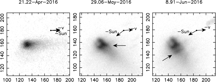
Observations of P/2016 G1 were scheduled immediately after the discovery alert, within our long-term GTC program of activated asteroids observations. CCD images of P/2016 G1 have been obtained under photometric and excellent seeing conditions on the nights of 20 April, 28 May, and 8 June 2016. The images were obtained using a Sloan $r^{\prime}$ filter in the Optical System for Image and Low Resolution Integrated Spectroscopy (OSIRIS) camera-spectrograph (Cepa et al., 2000; Cepa, 2010) at the GTC. The plate scale was 0.254$\arcsec$ px^-1. The images were bias subtracted, flat-fielded, and their flux was calibrated using standard stars from Smith et al. (2002). Those stars are observed with a slight defocus applied to the telescope in order to get high S/N in one second exposures, needed to avoid shutter non-uniformity effects in the photometry (that is accurate to 1% level). A median stack image was produced for each night of observation from the available frames. These images were converted from mag arcsec^-2 to solar disk intensity units (the output of our Monte Carlo dust tail code) by setting $r_{\odot}^{\prime}$=–26.95, obtained assuming $V_{\odot}$=–26.75 and $(B-V)_{\odot}$=0.65 (Cox, 2000), and the photometric relations from Fukugita et al. (1996). The log of the observations is presented in Table 1. This table includes the date of the observations (in UT and in days to perihelion), the heliocentric ($R$) and geocentric ($\Delta$) distances, the solar phase angle ($\alpha$), the position angle of the Sun to comet radius vector (PsAng), and the angle between the Earth and the asteroid orbital plane (PlAng). The reduced images are shown in Figure 1, in the conventional North-up, East-to-the-left orientation, and showing the directions of the Sun and orbital motion of the object.

The elevation of the Earth above the asteroid orbital plane ranges from nearly edge-on view (PlAng=–0.9^∘ on April 21) to PlAng=–6.1^∘ on June 8, allowing different viewing angles of the tail for an adequate analysis in terms of dust tail models. The conspicuous appearance of the object, with the lack of a central condensation (nucleus), and an inverted-C-shaped head with some westward extension that becomes apparent as PlAng becomes larger and larger, immediately suggest a likely disruptive phenomenon as the cause of the observed activity. Dust motion between the first and last observation can also contribute to the morphology changes. In those images, no small condensations that could be attributed to small fragments, (as detected for P/2013 R3 or P/2012 F5, see Jewitt et al., 2014; Drahus et al., 2015), are seen, however. The limiting magnitude with OSIRIS Sloan r^′ filter for getting a signal-to-noise ratio S/N=3, assuming a dark background, a seeing disk of FWHM=1.0$\arcsec$, and an airmass of 1.2, would be, for the total exposure time of 1080 s of the night of 28 May, 2016, of r^′=25.8 (see http://www.gtc.iac.es/instruments/osiris/). For the observational geometric conditions of that night (see Table 1), a spherical body of 47 m in radius, characterized by a geometric albedo of 0.15, and a linear phase coefficient of 0.03 mag deg^-1, would have this magnitude. Hence, no parent body or fragments larger than that size would have been produced as a consequence of the asteroid activation. This is actually an optimistic size limit, however, since the limiting magnitude refers to a dark background, and not to a source located within a bright background coma.

3 The Model

To perform a theoretical interpretation of the obtained images in terms of the dust physical parameters, we used our Monte Carlo dust tail code, which has been used previously on several works on activated asteroids and comets, including comet 67P/Churyumov-Gerasimenko, the Rosetta target (e.g., Moreno et al., 2016a). This model computes the dust tail brightness of a comet or activated asteroid by adding up the contribution to the brightness of each particle ejected from the parent nucleus. The particles, after leaving the object’s surface, are ejected to space experiencing the solar gravity and radiation pressure. The nucleus gravity force is neglected, a valid approximation for small-sized objects. Then, the trajectories of the particles become Keplerian, having orbital elements which depend on their physical properties and ejection velocities (e.g. Fulle, 1989). In order to build up an usable representation of the individual images with the Monte Carlo procedure, we usually launch from 2$\times$10⁶ to 10⁷ particles. For a given set of dust parameters, three synthetic images corresponding to the observational parameters of table 1 are generated using separate Monte Carlo runs for each image.

The ratio of radiation pressure to the gravity forces exerted on each particle is given by the parameter $\beta=C_{pr}Q_{pr}/(2\rho r)$, where $C_{pr}$=1.19$\times$ 10^-3 kg m^-2, $Q_{pr}$ is the radiation pressure coefficient, and $\rho$ is the particle density. $Q_{pr}$ is taken as 1, as it converges to that value for absorbing particles of radius $r\gtrsim$1 $\mu$m (see e.g. Moreno et al., 2012, their Figure 5).

To make the problem tractable, a number of simplifying assumptions on the dust physical parameters must be made. Thus, the particle density is taken as 1000 kg m^-3, and the geometric albedo is set to $p_{v}$=0.15, a typical value for C-type asteroids. The assumption of a lower albedo would imply an increase in the derived loss rates to fit the observed brightness. For the particle phase function correction, we use a linear phase coefficient of 0.03 mag deg^-1, which is in the range of comet dust particles in the 1${}^{\circ}\leq\alpha\leq$ 30^∘ phase angle domain (Meech & Jewitt, 1987). A broad size distribution is assumed, with minimum and maximum particle radii set to 1 $\mu$m and 1 cm, respectively, and following a power-law function of index $\kappa$=–3. This index was found appropriate after repeated experimentation with the code, and it is within the range of previous estimates of the size distribution of particles ejected from activated asteroids and comets.

We assume isotropic ejection of the particles, which will provide a first order description of the dust model parameters, although some of them such as the dust size distribution, the ejected dust mass, and the timing of event, can be estimated using such approximation.

The ejection velocity of the particles will depend on the activation mechanism involved, which, in principle, is unknown. However, the object is located in the inner region of the main belt, having a small semi-major axis, suggesting that ice sublimation is unlikely the driver of the activity. Recent results on activated asteroid P/2015 X6 (Moreno et al., 2016b) reveal that a random function for the velocities of the form $v=v_{1}+\zeta v_{2}$, where $\zeta$ is a random number in the $[0,1]$ interval, and $v_{1}$ and $v_{2}$ are fitting parameters, produced adequate results. Hence, to limit the number of free parameters, we assume that velocity law.

For the dust loss rate as a function of time, we adopt a half-Gaussian function whose maximum is the peak dust-loss rate ($\dot{M}_{0}$), located at the event onset ($t_{0}$). The half-width at half-maximum of the Gaussian (HWHM) is a measure of the effective time span of the event.

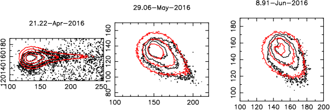
Summarizing, we have selected five fitting parameters for the isotropic model: the two dust ejection velocity parameters ($v_{1}$ and $v_{2}$) and the three parameters associated to the dust loss rate function ($\dot{M}_{0}$, $t_{0}$, and HWHM). The model analysis, aimed at finding the best-fit set of parameters, is conducted by the downhill simplex method (Nelder & Mead, 1965), using the FORTRAN implementation described in Press et al. (1992). A preliminary, zero-th order analysis, of the images is first performed by building a syndyne-synchrone map (Finson & Probstein, 1968) for each observing date. As an example, the synchrone map for the 28 May 2016 image is displayed in Figure 2. It is clear from the plot that the time span the asteroid has been active should be between around –300 to –360 days to perihelion, and its duration cannot be much longer than the time difference of $\sim$60 days, otherwise the dust cloud would have been much more fan broadly. Hence, parameter $t_{0}$ was assumed in the five-dimensional starting simplex to vary between these limits. In addition, it is also clear from the synchrone plot that a very short emission scenario (say, less than a day) can also be ruled out owing to the observed tail width.

All the other parameters were assumed to vary broadly between physically reasonable limits. The fits are characterized by the parameter $\chi=\sum\sigma_{i}$, where the summation is extended to the three images under consideration, and $\sigma_{i}=\sqrt{(\sum[\log(I_{obs}(i))-\log(I_{fit}(i))]^{2}/N(i))}$, where $I_{obs}(i)$ and $I_{fit}(i)$ are the observed and modeled tail brightness, and $N(i)$ is the number of pixels of image $i$. We work on the logarithm of intensities in order to give a much more similar weight to the outermost image isophotes and the innermost ones than would be done using simply intensities, owing to the brightness gradient toward the innermost portion of the object.

4 Results and discussion

Using the procedure described in the previous section, we found the following best-fit parameters: $\dot{M}_{0}$=7.6 kg s^-1, $t_{0}$=–350 days, HWHM=24 days, $v_{1}$=0.015 m s^-1 and $v_{2}$=0.122 m s^-1. The total dust mass ejected was 1.7$\times$10⁷ kg, all this mass being emitted before the first observation of April 21, 2016.

The best-fit images are compared to the observed ones in Figure 3. This best-fit model has $\chi$=0.109. As in our analysis of activated asteroid P/2015 X6 (Moreno et al., 2016b), acceptable solutions are considered only when $\chi\leq$0.15. These limiting values of $\chi$ provide lower and upper limits to the derived best-fit parameters. Thus, for the timing parameters $t_{0}$ and HWHM, we obtain $t_{0}$=–350${}^{+10}_{-30}$ days, and HWHM=24${}^{+10}_{-7}$ days. This implies a relatively short-duration event, that, in principle, can be associated to a wide range of phenomena. The particle velocities found are very small, ranging from 0.015 to 0.14 m s^-1. The mean value of these velocities ($\sim$ 0.08 m s^-1) is comparable to the escape velocity an object of 35 m in radius and 3000 kg m^-3 in density. However, as stated before, the minimum detectable object radius is $\sim$50 m. This implies that a parent nucleus, or possible fragments, smaller than that size would have remained unobserved. Higher resolution and better sensitivity images (such as provided by the Hubble Space Telescope) are clearly needed to search for fragments.

Regarding the particle size limits, we must note that the upper limit assumed of $r_{max}$=1 cm is constraining the total mass ejected to $\sim$1.7$\times$10⁷ kg. However, if this upper limit is increased, the amount of mass ejected would be larger accordingly. For instance, increasing $r_{max}$ to 10 cm, we can obtain fits of comparable quality to those shown in Figure 3, just by varying the power index of the size distribution from $\kappa$=–3.0 to $\kappa$=–3.2, and the peak mass loss rate from $\dot{M}_{0}$=7.6 kg s^-1 to $\dot{M}_{0}$=32 kg s^-1. In consequence, the amount of dust mass calculated from our standard isotropic model would be actually a lower limit to the total mass emitted, if particles larger than 1 cm in radius were ejected.

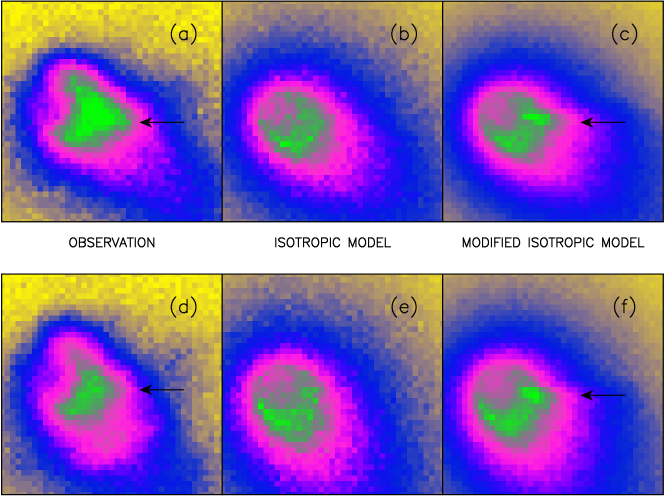
In order to gain more insight into the possible activation mechanism(s), we note that while the inverted-C shape feature observed on May 29 and June 8 images are approximately mimicked with the isotropic model, the westward extension is, as expected, not reproduced in the simulated images, implying some asymmetry in the ejection pattern. After some experimentation with the code, we found that if right at the beginning of the event all the ejected material is directed towards a specific direction and during a very short time interval, instead of being emitted isotropically, we could then simulate that brightness feature. To accomplish this task, we introduce a cometocentric reference system of unit vectors ($u_{r}$, $u_{\theta}$, $u_{z}$), where $u_{r}$ points away from the Sun, $u_{\theta}$ is perpendicular to $u_{r}$, located on the orbital plane, in the sense opposite to the comet motion, and $u_{z}$ is perpendicular to the orbit plane. We found that in order to simulate the westward brightness feature, the direction of ejection must satisfy u${}_{r}\sim$1, i.e., pointing away from the Sun. Figure 4 shows the effect of ejection around a specific direction given by $u_{r}\sim$0.98, $u_{\theta}\sim$0.18, $u_{z}\sim$0.08 on the May and June images (modified isotropic model), compared with the nominal isotropic model. The duration of this early dust mass ejection was set to 9 hours, but the feature could be equally simulated assuming a shorter time interval, as long as the total mass ejected in that direction keeps constant. This could be interpreted as the result of an impact whose ejecta is directed along that direction. Although such event should have likely generated an ejection cone with an aperture $\sim$40^∘, we cannot, however, describe the direction pattern more accurately owing to the limited spatial resolution of the measurements and the viewing angles restriction inherent to Earth-based observations. The dust mass ejected in that privileged direction would be $\sim$2.4$\times$10⁵ kg. We note that, although a fraction of the ejected material would have probably traveled at much higher velocity, in a collision most of the material is actually ejected at lower velocities (Housen and Holsapple, 2011). The impact would have induced a partial destruction of the asteroid, with dust grains being emitted to space nearly isotropically while the body is being torn apart. The presence of small fragments that could be generated in the disruption process can only be assessed with more sensitive instrumentation.

5 Conclusions

From the GTC imaging data and the Monte Carlo dust tail modeling of the activated asteroid P/2016 G1, we arrived to the following conclusions:

1) Asteroid P/2016 G1 was activated 350${}^{+10}_{-30}$ days before perihelion, i.e., around 10th February 2016. The activity had a duration of 24${}^{+10}_{-30}$ days (HWHM), so that no dust has been produced since our first observation of April 21, 2016. The total dust mass emitted was at least $\sim$2$\times$10⁷ kg, with a maximum level of activity of $\sim$8 kg s^-1. These parameters were estimated assuming a power-law size distribution of particles between 1 $\mu$m and 1 cm, with power index of $\kappa$=–3.0, geometric albedo of 0.15, and being emitted isotropically from an otherwise undetected nucleus. The calculated peak and total dust mass are lower limits, as if larger values for the maximum particle size were assumed, these quantities would increase. In addition, if different values for the geometric albedo and/or for the density of the particles were assumed, these quantities would also change accordingly.

2) While the inverted-C feature which is apparent in the out-of-plane images of May 29 and June 8, 2016 is approximately mimicked by the isotropic ejection model, a westward brightness feature cannot be reproduced with that model. However, if some dust mass is ejected from a specified direction right at the time of activation, which turns out to be approximately along the Sun-to-asteroid vector, that feature becomes apparent in the simulations. We speculate that this dust ejection could be associated to an impact, and that the subsequent modeled activity is due to the asteroid partial or total disruption. The impact itself had produced the ejection of some 2.4$\times$10⁵ kg of dust.

3) The inferred ejection velocities of the dust particles are very small, in the range of 0.015 to 0.14 m s^-1, with an average value of $\sim$0.08 m s^-1, corresponding to the escape velocity of an object of 35 m radius and 3000 kg m^-3 density. An object of that size would have been remained well below the detection limit of the images acquired, so that we cannot assure whether fragments of that size or smaller could exist in the vicinity of the dust cloud. Deeper imaging of the object is clearly needed to assess this fact and to determine the fragment dynamics.

Figure 1: Median stack images of P/2016 G1 obtained with the OSIRIS instrument of the 10.4m GTC through a Sloan $r^{\prime}$ filter, at the indicated dates. North is up, East to the left. The directions opposite to Sun and the negative of the orbital velocity motion are shown. The arrow in the middle of central panel indicates the westward feature that emerges from the inverted C-shaped mentioned in the text. The dimensions of the panels (from left to right, in km projected on the sky at the asteroid distance) are 27930$\times$27930, 26305$\times$26305, and 27025$\times$27025. The images are stretched linearly in brightness, with maximum intensity levels, from left to right, of 8$\times$10^-14, 5$\times$10^-14, and 4$\times$10^-14 solar disk intensity units. Faint trailed stars are apparent near the head of the object, perpendicular to the tail, in the 8.91 June 2016 image, the brightest one being indicated by an arrow.

Figure 2: Synchrone map corresponding to the 29.06 May 2016 image overplotted on the contour map (thin solid lines). Synchrones (thick solid lines) correspond to –380 to –260 days to perihelion, in steps of 20 days, as labeled. The directions to the Sun and the orbital velocity motion of the asteroid are indicated.

Figure 3: Measured (black) and modeled (red) isophotes for the three images analyzed. Innermost isophote levels are 4$\times$10^-14 (left panel) and 2$\times$10^-14 (center and right panels) solar disk intensity units, and decrease in factors of two outwards.

Figure 4: Observed and simulated images in the vicinity of the head region on May 29.06 (upper panels, a, b, and c) and June 8.91 (lower panels, d, e, and f). The observations are on panels (a) and (d). The isotropic ejection model images are on panels (b) and (e), and the modified isotropic model including early dust ejection in the direction of unit vector (0.98,0.18,0.08) in the cometocentric frame are on panels (c) and (f). The arrows indicate the location of the westward extension described in the text, which appears in the observations and in the modified isotropic model, but not in the isotropic model. The upper panels have dimensions of 10522$\times$10522 km, and the lower panels 10810$\times$10810 km.

Table 1: Log of the observations

UT (Start)	Days to	No. of	Total	Seeing	R	$\Delta$	$\alpha$	PsAng	PlAng
YYYY/MM/DD HH:MM	perihelion	images	exp. time (s)	FWHM(″)	(AU)	(AU)	(∘)	(∘)	(∘)
2016/04/21 05:18	–297	20	600	1.0	2.473	1.516	9.13	268.8	–0.909
2016/05/29 01:24	–242	6	1080	0.9	2.386	1.428	10.27	127.4	–5.365
2016/06/08 21:45	–231	5	900	0.7	2.362	1.467	14.83	120.5	–6.128

References

- Cox (2000) Cox, A.N. 2000, Allen’s Astrophysical Quantities, fourth edition. Springer-Verlag.
- Cepa et al. (2000) Cepa, J., Aguiar, M., Escalera, V. et al. 2000, Poc. SPIE, 4008, 623
- Cepa (2010) Cepa, J. 2010, Highlights of Spanish Astrophysics V, Astrophysics and Space Science Proceedings, Springer-Verlag, p. 15
- Drahus et al. (2015) Drahus, M., Waniak, W., Tendulkar, S. et al. 2015, ApJ, 802, L8
- Finson & Probstein (1968) Finson, M., & Probstein, R. 1968, ApJ, 154, 327
- Fulle (1989) Fulle, M., 1989, A&A, 217, 283
- Fukugita et al. (1996) Fukugita, M., Ichikawa, T., Gunn, J.E., et al. 1996, AJ, 111, 1748
- Housen and Holsapple (2011) Housen, K.R. & Holsapple, K.A. 2011, Icarus, 211, 856
- Hsieh et al. (2004) Hsieh, H.H., Jewitt, D., and Fernández, Y. 2004, AJ, 127, 2997
- Jewitt et al. (2014) Jewitt, D., Agarwal, J., Li, J., et al. 2014, ApJ, 784, L1
- Jewitt et al. (2015) Jewitt, D., Agarwal, J., Hsieh, H. 2015, Asteroids IV (Tucson, AZ: Univ. Arizona Press)
- Kresak (1982) Kresak, L. 1982 BAICz, 33, 104
- Meech & Jewitt (1987) Meech, K. J., & Jewitt, D. C., 1987, A&A, 187, 585
- Moreno et al. (2012) Moreno, F., Pozuelos, F., Aceituno, F., et al. 2012, ApJ, 752, 136
- Moreno et al. (2016a) Moreno, F., Snodgrass, C., Hainaut, O., et al. 2016, A&A, 587, A155
- Moreno et al. (2016b) Moreno, F., Licandro, J., Cabrera-Lavers, A., et al. 2016 ApJ, in press
- Nelder & Mead (1965) Nelder, J. A., & Mead, R. 1965, Comput. J., 7, 308
- Press et al. (1992) Press, W.H., Teukolsky, S.A., Vetterling, W.T., & Flannery, B.P. 1992, in Numerical Recipes in FORTRAN (Cambridge: Cambridge Univ. Press), 402
- Smith et al. (2002) Smith, J.A., Tucker, D.L., Kent, S., et al. 2002, AJ, 123, 2121
- Weryk & Wainscoat (2016) Weryk, R. & Wainscoat, R.J. 2016, Central Bureau for Astronomical Telegrams, 4269