Implications of Fermionic Dark Matter on recent neutrino oscillation data***I would like to thank Rukmani Mohanta for helpful suggestions. This work is supported by DST-Inspire Fellowship division - IF130927.

Shivaramakrishna Singirala  School of Physics, University of Hyderabad, Hyderabad - 500046, India
Abstract

We investigate flavor phenomenology and dark matter in the context of scotogenic model. In this model, the neutrino masses are generated through radiative corrections at one-loop level. Considering the neutrino mixing matrix to be of tri-bimaximal form with additional perturbations to accommodate the recently observed non-zero value of reactor mixing angle ΞΈ13subscriptπœƒ13\theta_{13}, we obtain the relation between various neutrino oscillation parameters and the model parameters. Working in degenerate heavy neutrino mass spectrum, we obtain light neutrino masses obeying normal hierarchy and also study the relic abundance of fermionic dark matter candidate including coannihilation effects. A viable parameter space is thus obtained, consistent with neutrino oscillation data, relic abundance and various lepton flavor violating decays such as ℓα→ℓβ​γ→subscriptℓ𝛼subscriptℓ𝛽𝛾\ell_{\alpha}\to\ell_{\beta}\gamma and β„“Ξ±β†’3​ℓβ→subscriptℓ𝛼3subscriptℓ𝛽\ell_{\alpha}\to 3\,\ell_{\beta}.

Keywords: Dark matter, Neutrino mixing, Lepton flavor violation.

pacs:
13.35.βˆ’formulae-sequence13.3513.35.-r, 14.60.14.6014.60.Pq, 95.35.+formulae-sequence95.3595.35.+d

I Introduction

Standard model (SM) of particle physics has been very successful in explaining physics at the fundamental level. However there are still many open questions for which it does not provide any satisfactory answer. The existence of dark matter (DM) and the observation of non-zero neutrino masses stand as few of the robust evidences for physics beyond the standard model.

Considerable progress has been made in the determination of neutrino mass square differences and mixing parameters from the data of various solar and atmospheric neutrino oscillation experiments. Theoretically, the smallness of neutrino mass can be generally explained by the well known seesaw mechanisms namely: type-I t1 , type-II t2 , type-III t3 and radiative seesaw ma . In standard parametrization, the mechanism of mixing can be described by unitary Pontecorvo-Maki-Nakagawa-Sakata (PMNS) matrix VP​M​N​Ssubscript𝑉𝑃𝑀𝑁𝑆V_{PMNS} pmns written in terms of three rotation angles ΞΈ12subscriptπœƒ12\theta_{12}, ΞΈ23subscriptπœƒ23\theta_{23}, ΞΈ13subscriptπœƒ13\theta_{13} and three CP-violating phases namely Ξ΄C​Psubscript𝛿𝐢𝑃\delta_{CP} (Dirac type) and ρ,ΟƒπœŒπœŽ\rho,\sigma (Majorana type) as

VP​M​N​S≑UP​M​N​Sβ‹…PΞ½=(c12​c13s12​c13s13​eβˆ’i​δC​Pβˆ’s12​c23βˆ’c12​s13​s23​ei​δC​Pc12​c23βˆ’s12​s13​s23​ei​δC​Pc13​s23s12​s23βˆ’c12​s13​c23​ei​δC​Pβˆ’c12​s23βˆ’s12​s13​c23​ei​δC​Pc13​c23)​PΞ½,subscript𝑉𝑃𝑀𝑁𝑆⋅subscriptπ‘ˆπ‘ƒπ‘€π‘π‘†subscriptπ‘ƒπœˆsubscript𝑐12subscript𝑐13subscript𝑠12subscript𝑐13subscript𝑠13superscript𝑒𝑖subscript𝛿𝐢𝑃subscript𝑠12subscript𝑐23subscript𝑐12subscript𝑠13subscript𝑠23superscript𝑒𝑖subscript𝛿𝐢𝑃subscript𝑐12subscript𝑐23subscript𝑠12subscript𝑠13subscript𝑠23superscript𝑒𝑖subscript𝛿𝐢𝑃subscript𝑐13subscript𝑠23subscript𝑠12subscript𝑠23subscript𝑐12subscript𝑠13subscript𝑐23superscript𝑒𝑖subscript𝛿𝐢𝑃subscript𝑐12subscript𝑠23subscript𝑠12subscript𝑠13subscript𝑐23superscript𝑒𝑖subscript𝛿𝐢𝑃subscript𝑐13subscript𝑐23subscriptπ‘ƒπœˆV_{PMNS}\equiv U_{PMNS}\cdot P_{\nu}=\left(\begin{array}[]{ccc}c_{12}c_{13}&s_{12}c_{13}&s_{13}e^{-i\delta_{CP}}\\ -s_{12}c_{23}-c_{12}s_{13}s_{23}e^{i\delta_{CP}}&c_{12}c_{23}-s_{12}s_{13}s_{23}e^{i\delta_{CP}}&c_{13}s_{23}\\ s_{12}s_{23}-c_{12}s_{13}c_{23}e^{i\delta_{CP}}&-c_{12}s_{23}-s_{12}s_{13}c_{23}e^{i\delta_{CP}}&c_{13}c_{23}\end{array}\right)P_{\nu}\;, (1)

where ci​j≑cos⁑θi​jsubscript𝑐𝑖𝑗subscriptπœƒπ‘–π‘—c_{ij}\equiv\cos\theta_{ij}, si​j≑sin⁑θi​jsubscript𝑠𝑖𝑗subscriptπœƒπ‘–π‘—s_{ij}\equiv\sin\theta_{ij} and Pν≑{ei​ρ,ei​σ,1}subscriptπ‘ƒπœˆsuperscriptπ‘’π‘–πœŒsuperscriptπ‘’π‘–πœŽ1P_{\nu}\equiv\{e^{i\rho},e^{i\sigma},1\} is a diagonal phase matrix. The mixing angles as well as the mass square differences have been well constrained by various neutrino oscillation experiments. Recently Daya Bay daya-bay1 ; daya-bay2 , RENO reno and T2K t2k collaborations have precisely measured the reactor mixing angle ΞΈ13subscriptπœƒ13\theta_{13} with a moderately large value. However, there are several missing pieces such as the neutrino mass hierarchy, the magnitude of the CP violating phase Ξ΄C​Psubscript𝛿𝐢𝑃\delta_{CP}, the absolute scale of the neutrino mass, and the nature of neutrinos (whether Dirac or Majorana). Various neutrino oscillation parameters derived from global analysis of recent oscillation data taken from Ref. osc are presented in Table-I.

Mixing Parameters Best Fit value 3​σ3𝜎3\sigma Range
sin2⁑θ12superscript2subscriptπœƒ12\sin^{2}\theta_{12} Β  0.3230.3230.323 Β 0.278β†’0.375β†’0.2780.3750.278\to 0.375
sin2⁑θ23superscript2subscriptπœƒ23\sin^{2}\theta_{23} (NO) Β  0.5670.5670.567 Β 0.392β†’0.643β†’0.3920.6430.392\to 0.643
sin2⁑θ13superscript2subscriptπœƒ13\sin^{2}\theta_{13} (NO) Β  0.02340.02340.0234 Β 0.0177β†’0.0294β†’0.01770.02940.0177\to 0.0294
Ξ΄CPsubscript𝛿CP\delta_{\rm CP} (NO) Β 1.34​π1.34πœ‹1.34\pi (0β†’2​π)β†’02πœ‹~{}(0\to 2\pi)~{}
Δ​m312/10βˆ’3​eV2​(NO)Ξ”superscriptsubscriptπ‘š312superscript103superscripteV2NO\Delta m_{31}^{2}/10^{-3}~{}{\rm eV}^{2}~{}({\rm NO}) Β  2.482.482.48 2.3β†’2.65β†’2.32.652.3\to 2.65
Δ​m212/10βˆ’5​eV2Ξ”superscriptsubscriptπ‘š212superscript105superscripteV2\Delta m_{21}^{2}/10^{-5}~{}{\rm eV}^{2} 7.607.607.60 7.11β†’8.18β†’7.118.187.11\to 8.18
Table 1: Best-fit values with their 3​σ3𝜎3\sigma ranges of the neutrino oscillation parameters from osc where NO indicates normal ordering.

On the other hand, the particle nature of dark matter is still a mystery till date. Recent survey of PLANCK planck reveal that DM constitutes about 26.8% of the total energy budget of the Universe. Various cosmological observations suggest that this unknown particle is non-relativistic in nature and is stable on cosmological time scales. Numerous beyond SM scenarios study DM phenomenology by imposing additional discrete symmetry such as R-parity, Z2subscript𝑍2Z_{2} symmetry etc. Weakly Interacting Massive Particle (WIMP miracle) is the best motivated candidate of DM. They are massive particles with cross section approximately the order of weak interaction cross section.

It would be interesting to study the extensions of standard model that can relate these two issues. Scotogenic model proposed by Ma ma is one among such frameworks in which neutrino mass generation involves the interaction with dark matter. In this model an unbroken discrete symmetry forbids neutrino attaining a tree level mass and also assures the stability of DM particle. It is a suitable platform to simultaneously explain neutrino oscillation data and DM phenomenology.

In this work, we consider the scotogenic model to correlate some of the neutrino oscillation parameters, like the mass square differences and the mixing angles with the model parameters. We examine the neutrino radiative mass matrix using the mixing matrix of TBM type with added perturbation to achieve large ΞΈ13subscriptπœƒ13\theta_{13}. We solve for suitable flavor structure to study neutrino phenomenology. We then use the best fit values on neutrino oscillation parameters to constrain the parameter space of this model. In addition, we study DM relic abundance choosing the lightest odd particle as the DM candidate. We scan over entire parameter space of the model imposing the constraints from neutrino data, DM observables and lepton flavor violating decays.

The paper is organized as follows. In section II we describe the scotogenic model. In section III we diagonalize the neutrino radiative mass matrix and obtain solutions to explain neutrino oscillation data. The fermionic DM relic abundance considering the coannihilation effects is studied in section IV and then in section V we estimate the branching ratios of various LFV decays. We conclude our discussion in section VI.

II Scotogenic model

Scotogenic model is a minimal extension of standard model with an additional inert scalar doublet Ξ·πœ‚\eta and three heavy Majorana right-handed neutrinos Nisubscript𝑁𝑖N_{i} (i=1,2,3𝑖123i=1,2,3). The potential is imposed with a discrete symmetry under which all the new particles i.e., Nisubscript𝑁𝑖N_{i} and Ξ·πœ‚\eta are odd and SM particles are even. The unbroken discrete symmetry guarantees the coupling of the inert doublet to fermions vanish and doesn’t get a vacuum expectation value (VEV). While the SM Higgs doublet Ο•italic-Ο•\phi obtains a VEV βŸ¨Ο•0⟩=vdelimited-⟨⟩superscriptitalic-Ο•0𝑣\langle\phi^{0}\rangle=v by the spontaneous symmetry breaking of S​U​(2)LΓ—U​(1)Yπ‘†π‘ˆsubscript2πΏπ‘ˆsubscript1π‘ŒSU(2)_{L}\times U(1)_{Y} global symmetry. This model is rich in phenomenology providing scalar and fermionic dark matter candidates. Scalar dark matter in this model has been studied extensively in literature lopez ; barbieri ; Gustafsson .

The scalar potential of this model is given by suematsu

V𝑉\displaystyle V =\displaystyle= mΟ•2​ϕ†​ϕ+mΞ·2​η†​η+12​λ1​(ϕ†​ϕ)2+12​λ2​(η†​η)2+Ξ»3​(ϕ†​ϕ)​(η†​η)superscriptsubscriptπ‘šitalic-Ο•2superscriptitalic-ϕ†italic-Ο•superscriptsubscriptπ‘šπœ‚2superscriptπœ‚β€ πœ‚12subscriptπœ†1superscriptsuperscriptitalic-ϕ†italic-Ο•212subscriptπœ†2superscriptsuperscriptπœ‚β€ πœ‚2subscriptπœ†3superscriptitalic-ϕ†italic-Ο•superscriptπœ‚β€ πœ‚\displaystyle m_{\phi}^{2}\phi^{\dagger}\phi+m_{\eta}^{2}\eta^{\dagger}\eta+{1\over 2}\lambda_{1}(\phi^{\dagger}\phi)^{2}+{1\over 2}\lambda_{2}(\eta^{\dagger}\eta)^{2}+\lambda_{3}(\phi^{\dagger}\phi)(\eta^{\dagger}\eta) (2)
+\displaystyle+ Ξ»4​(ϕ†​η)​(η†​ϕ)+12​λ5​[(ϕ†​η)2+(η†​ϕ)2],subscriptπœ†4superscriptitalic-Ο•β€ πœ‚superscriptπœ‚β€ italic-Ο•12subscriptπœ†5delimited-[]superscriptsuperscriptitalic-Ο•β€ πœ‚2superscriptsuperscriptπœ‚β€ italic-Ο•2\displaystyle\lambda_{4}(\phi^{\dagger}\eta)(\eta^{\dagger}\phi)+{1\over 2}\lambda_{5}[(\phi^{\dagger}\eta)^{2}+(\eta^{\dagger}\phi)^{2}],

where the two scalar doublets Ο•italic-Ο•\phi and Ξ·πœ‚\eta are defined as

Ο•=(Ο•+Ο•0),Ξ·=(Ξ·+Ξ·0).formulae-sequenceitalic-Ο•superscriptitalic-Ο•superscriptitalic-Ο•0πœ‚superscriptπœ‚superscriptπœ‚0\phi=\left(\begin{array}[]{c}\phi^{+}\\ \phi^{0}\\ \end{array}\right),\qquad\eta=\left(\begin{array}[]{c}\eta^{+}\\ \eta^{0}\\ \end{array}\right). (3)

After spontaneous symmetry breaking, the masses of the charged component (Ξ·+superscriptπœ‚\eta^{+}) and neutral components of Ξ·0=(Ξ·R+i​ηI)/2superscriptπœ‚0subscriptπœ‚π‘…π‘–subscriptπœ‚πΌ2\eta^{0}=(\eta_{R}+i\eta_{I})/\sqrt{2} are given by

mΞ·+2=mΞ·2+Ξ»3​v2,superscriptsubscriptπ‘šsuperscriptπœ‚2superscriptsubscriptπ‘šπœ‚2subscriptπœ†3superscript𝑣2\displaystyle m_{\eta^{+}}^{2}=m_{\eta}^{2}+\lambda_{3}v^{2},
mR2=mΞ·2+(Ξ»3+Ξ»4+Ξ»5)​v2,superscriptsubscriptπ‘šπ‘…2superscriptsubscriptπ‘šπœ‚2subscriptπœ†3subscriptπœ†4subscriptπœ†5superscript𝑣2\displaystyle m_{R}^{2}=m_{\eta}^{2}+(\lambda_{3}+\lambda_{4}+\lambda_{5})v^{2},
mI2=mΞ·2+(Ξ»3+Ξ»4βˆ’Ξ»5)​v2.superscriptsubscriptπ‘šπΌ2superscriptsubscriptπ‘šπœ‚2subscriptπœ†3subscriptπœ†4subscriptπœ†5superscript𝑣2\displaystyle m_{I}^{2}=m_{\eta}^{2}+(\lambda_{3}+\lambda_{4}-\lambda_{5})v^{2}. (4)

The Yukawa Lagrangian of this model is suematsu

β„’N=Ni¯​iβ€‹βˆ‚/PR​Ni+(Dμ​η)†​(Dμ​η)βˆ’Mi2​Nic¯​PR​Ni+hα​i​ℓα¯​η†​PR​Ni+h.c.,formulae-sequencesubscriptℒ𝑁¯subscript𝑁𝑖𝑖subscript𝑃𝑅subscript𝑁𝑖superscriptsubscriptπ·πœ‡πœ‚β€ superscriptπ·πœ‡πœ‚subscript𝑀𝑖2Β―superscriptsubscript𝑁𝑖𝑐subscript𝑃𝑅subscript𝑁𝑖subscriptβ„Žπ›Όπ‘–Β―subscriptℓ𝛼superscriptπœ‚β€ subscript𝑃𝑅subscript𝑁𝑖hc\mathcal{L}_{N}=\overline{N_{i}}i\partial\!\!\!/\!\>P_{R}N_{i}+\left(D_{\mu}\eta\right)^{\dagger}\left(D^{\mu}\eta\right)-\frac{M_{i}}{2}\overline{N_{i}\>\!^{c}}P_{R}N_{i}+h_{\alpha i}\overline{\ell_{\alpha}}\eta^{\dagger}P_{R}N_{i}+\mathrm{h.c.}, (5)

where hα​isubscriptβ„Žπ›Όπ‘–h_{\alpha i} are the Yukawa couplings, α𝛼\alpha denotes the lepton flavor and Misubscript𝑀𝑖M_{i} are the masses of heavy neutrinos Nisubscript𝑁𝑖N_{i}.

In this model, neutrinos get their mass by loop correction called β€œradiative seesaw mechanism”. The corresponding neutrino mass matrix is given by

(β„³Ξ½)α​β=βˆ‘i=13hα​i​hβ​i​Λi,subscriptsubscriptβ„³πœˆπ›Όπ›½superscriptsubscript𝑖13subscriptβ„Žπ›Όπ‘–subscriptβ„Žπ›½π‘–subscriptΛ𝑖({\cal M}_{\nu})_{\alpha\beta}=\sum_{i=1}^{3}h_{\alpha i}h_{\beta i}\Lambda_{i}, (6)

where Ξ›isubscriptΛ𝑖\Lambda_{i} is defined as

Ξ›i=Ξ»5​v28​π2​Mi​I​(ri),I​(x)=x21βˆ’x2​(1+x21βˆ’x2​ln⁑x2),formulae-sequencesubscriptΛ𝑖subscriptπœ†5superscript𝑣28superscriptπœ‹2subscript𝑀𝑖𝐼subscriptπ‘Ÿπ‘–πΌπ‘₯superscriptπ‘₯21superscriptπ‘₯21superscriptπ‘₯21superscriptπ‘₯2superscriptπ‘₯2\Lambda_{i}=\frac{\lambda_{5}v^{2}}{8\pi^{2}M_{i}}I\left(r_{i}\right),\qquad I(x)=\frac{x^{2}}{1-x^{2}}\left(1+\frac{x^{2}}{1-x^{2}}\ln x^{2}\right), (7)

Here the parameters risubscriptπ‘Ÿπ‘–r_{i} are defined as ri=Mi/m0subscriptπ‘Ÿπ‘–subscript𝑀𝑖subscriptπ‘š0r_{i}=M_{i}/m_{0} and m02=(mR2+mI2)/2superscriptsubscriptπ‘š02superscriptsubscriptπ‘šπ‘…2superscriptsubscriptπ‘šπΌ22{m_{0}}^{2}=({m_{R}}^{2}+{m_{I}}^{2})/2. We take Ξ»5∼10βˆ’10similar-tosubscriptπœ†5superscript1010\lambda_{5}\sim 10^{-10}, a very small value in order to have correct neutrino masses and also probe for lepton flavor violation schmidt ; suematsu ; vicente1 ; vicente2 . We now diagonalize the radiative mass matrix (6) using PMNS matrix to explain neutrino oscillation data.

III Neutrino phenemenology

Various neutrino experiments confirmed that neutrinos have tiny mass and they oscillate from one flavor to another as they propagate. The phenomenon of neutrino oscillation is described by solar (ΞΈ12subscriptπœƒ12\theta_{12}), atmospheric (ΞΈ23subscriptπœƒ23\theta_{23}) and reactor (ΞΈ13subscriptπœƒ13\theta_{13}) mixing angles. Of these three rotation angles, two are large (ΞΈ12subscriptπœƒ12\theta_{12} and ΞΈ23subscriptπœƒ23\theta_{23}), and one is not so large (ΞΈ13subscriptπœƒ13\theta_{13}). Originally, it was believed that the reactor mixing angle would be very small and with this motivation numerous models were proposed which are generally based on some discrete flavor symmetries such as S3subscript𝑆3S_{3}, S4subscript𝑆4S_{4}, A4subscript𝐴4A_{4}, etc sym to explain the neutrino mixing pattern. For instance, the tri-bimaximal (TBM) mixing pattern tbm , a well motivated model having sin2⁑θ12=13superscript2subscriptπœƒ1213\sin^{2}\theta_{12}=\frac{1}{3} and sin2⁑θ23=12superscript2subscriptπœƒ2312\sin^{2}\theta_{23}=\frac{1}{2} which can be expressed in a generalized form as

UΞ½0=(cos⁑θsin⁑θ0βˆ’sin⁑θ2cos⁑θ212sin⁑θ2βˆ’cos⁑θ212),superscriptsubscriptπ‘ˆπœˆ0πœƒπœƒ0πœƒ2πœƒ212πœƒ2πœƒ212U_{\nu}^{0}=\left(\begin{array}[]{ccc}\cos\theta&\sin\theta&0\\ -\frac{\sin\theta}{\sqrt{2}}&\frac{\cos\theta}{\sqrt{2}}&\frac{1}{\sqrt{2}}\\ \frac{\sin\theta}{\sqrt{2}}&-\frac{\cos\theta}{\sqrt{2}}&\frac{1}{\sqrt{2}}\\ \end{array}\right), (8)

with θ≃35∘similar-to-or-equalsπœƒsuperscript35\theta\simeq 35^{\circ}. However, in TBM mixing pattern the value of ΞΈ13subscriptπœƒ13\theta_{13} turn out to be zero. After the experimental evidence of moderately large ΞΈ13subscriptπœƒ13\theta_{13}, it was found that adding suitable perturbation terms to the TBM mixing pattern can still describe the neutrino mixing pattern with sizeable ΞΈ13subscriptπœƒ13\theta_{13}. As discussed in sruthilaya , here we consider a simple perturbation matrix, i.e., a rotation matrix in 13 plane, which can provide the required corrections to the various mixing angles of TBM mixing matrix. Assuming the charged lepton mass matrix is diagonal (i.e., identity matrix), one can write the PMNS mixing matrix, which relates the flavor eigenstates to the corresponding mass eigenstates as

UP​M​N​S=UΞ½0​(cos⁑φ0eβˆ’i​΢​sin⁑φ010βˆ’ei​΢​sin⁑φ0cos⁑φ).subscriptπ‘ˆπ‘ƒπ‘€π‘π‘†superscriptsubscriptπ‘ˆπœˆ0πœ‘0superscriptπ‘’π‘–πœπœ‘010superscriptπ‘’π‘–πœπœ‘0πœ‘U_{PMNS}=U_{\nu}^{0}\left(\begin{array}[]{ccc}\cos\varphi&0&e^{-i\zeta}\sin\varphi\\ 0&1&0\\ -e^{i\zeta}\sin\varphi&0&\cos\varphi\\ \end{array}\right). (9)

In our work, we consider the phase ΢𝜁\zeta to be zero for convenience. Now we diagonalize the mass matrix (6) by the mixing matrix (9) using the relation UP​M​N​ST​ℳν​UP​M​N​S=diag​(m1,m2,m3).superscriptsubscriptπ‘ˆπ‘ƒπ‘€π‘π‘†π‘‡subscriptβ„³πœˆsubscriptπ‘ˆπ‘ƒπ‘€π‘π‘†diagsubscriptπ‘š1subscriptπ‘š2subscriptπ‘š3U_{PMNS}^{T}{\cal M}_{\nu}U_{PMNS}={\rm diag}(m_{1},m_{2},m_{3}). This in turn provides the following conditions (vanishing off-diagonal elements of the mass matrix) to be satisfied:

βˆ‘i=13he​i22​sin⁑2​θ​cos⁑φ+he​i​(hμ​iβˆ’hτ​i)2​cos⁑2​θ​cosβ‘Ο†βˆ’(hμ​iβˆ’hτ​i)24​sin⁑2​θ​cos⁑φsuperscriptsubscript𝑖13superscriptsubscriptβ„Žπ‘’π‘–222πœƒπœ‘subscriptβ„Žπ‘’π‘–subscriptβ„Žπœ‡π‘–subscriptβ„Žπœπ‘–22πœƒπœ‘superscriptsubscriptβ„Žπœ‡π‘–subscriptβ„Žπœπ‘–242πœƒπœ‘\displaystyle\sum_{i=1}^{3}\frac{h_{ei}^{2}}{2}\sin 2\theta\cos\varphi+\frac{h_{ei}(h_{\mu i}-h_{\tau i})}{\sqrt{2}}\cos 2\theta\cos\varphi-\frac{(h_{\mu i}-h_{\tau i})^{2}}{4}\sin 2\theta\cos\varphi
βˆ’he​i​(hμ​i+hτ​i)2​sin⁑θ​sinβ‘Ο†βˆ’(hμ​i2βˆ’hτ​i2)2​cos⁑θ​sin⁑φ=0,subscriptβ„Žπ‘’π‘–subscriptβ„Žπœ‡π‘–subscriptβ„Žπœπ‘–2πœƒπœ‘superscriptsubscriptβ„Žπœ‡π‘–2superscriptsubscriptβ„Žπœπ‘–22πœƒπœ‘0\displaystyle-\frac{h_{ei}(h_{\mu i}+h_{\tau i})}{\sqrt{2}}\sin\theta\sin\varphi-\frac{(h_{\mu i}^{2}-h_{\tau i}^{2})}{2}\cos\theta\sin\varphi=0, (10a)
βˆ‘i=13he​i22​sin⁑2​θ​sin⁑φ+he​i​(hμ​iβˆ’hτ​i)2​cos⁑2​θ​sinβ‘Ο†βˆ’(hμ​iβˆ’hτ​i)24​sin⁑2​θ​sin⁑φsuperscriptsubscript𝑖13superscriptsubscriptβ„Žπ‘’π‘–222πœƒπœ‘subscriptβ„Žπ‘’π‘–subscriptβ„Žπœ‡π‘–subscriptβ„Žπœπ‘–22πœƒπœ‘superscriptsubscriptβ„Žπœ‡π‘–subscriptβ„Žπœπ‘–242πœƒπœ‘\displaystyle\sum_{i=1}^{3}\frac{h_{ei}^{2}}{2}\sin 2\theta\sin\varphi+\frac{h_{ei}(h_{\mu i}-h_{\tau i})}{\sqrt{2}}\cos 2\theta\sin\varphi-\frac{(h_{\mu i}-h_{\tau i})^{2}}{4}\sin 2\theta\sin\varphi
+he​i​(hμ​i+hτ​i)2​sin⁑θ​cos⁑φ+(hμ​i2βˆ’hτ​i2)2​cos⁑θ​cos⁑φ=0,subscriptβ„Žπ‘’π‘–subscriptβ„Žπœ‡π‘–subscriptβ„Žπœπ‘–2πœƒπœ‘superscriptsubscriptβ„Žπœ‡π‘–2superscriptsubscriptβ„Žπœπ‘–22πœƒπœ‘0\displaystyle+\frac{h_{ei}(h_{\mu i}+h_{\tau i})}{\sqrt{2}}\sin\theta\cos\varphi+\frac{(h_{\mu i}^{2}-h_{\tau i}^{2})}{2}\cos\theta\cos\varphi=0, (10b)
βˆ‘i=13he​i22​cos2⁑θ​sin⁑2β€‹Ο†βˆ’he​i​(hμ​iβˆ’hτ​i)2​2​sin⁑2​θ​sin⁑2​φ+(hμ​iβˆ’hτ​i)24​sin2⁑θ​sin⁑2​φsuperscriptsubscript𝑖13superscriptsubscriptβ„Žπ‘’π‘–22superscript2πœƒ2πœ‘subscriptβ„Žπ‘’π‘–subscriptβ„Žπœ‡π‘–subscriptβ„Žπœπ‘–222πœƒ2πœ‘superscriptsubscriptβ„Žπœ‡π‘–subscriptβ„Žπœπ‘–24superscript2πœƒ2πœ‘\displaystyle\sum_{i=1}^{3}\frac{h_{ei}^{2}}{2}\cos^{2}\theta\sin 2\varphi-\frac{h_{ei}(h_{\mu i}-h_{\tau i})}{2\sqrt{2}}\sin 2\theta\sin 2\varphi+\frac{(h_{\mu i}-h_{\tau i})^{2}}{4}\sin^{2}\theta\sin 2\varphi
+he​i​(hμ​i+hτ​i)2​cos⁑θ​cos⁑2β€‹Ο†βˆ’(hμ​i2βˆ’hτ​i2)2​sin⁑θ​cos⁑2β€‹Ο†βˆ’(hμ​i+hτ​i)24​sin⁑2​φ=0.subscriptβ„Žπ‘’π‘–subscriptβ„Žπœ‡π‘–subscriptβ„Žπœπ‘–2πœƒ2πœ‘superscriptsubscriptβ„Žπœ‡π‘–2superscriptsubscriptβ„Žπœπ‘–22πœƒ2πœ‘superscriptsubscriptβ„Žπœ‡π‘–subscriptβ„Žπœπ‘–242πœ‘0\displaystyle+\frac{h_{ei}(h_{\mu i}+h_{\tau i})}{\sqrt{2}}\cos\theta\cos 2\varphi-\frac{(h_{\mu i}^{2}-h_{\tau i}^{2})}{2}\sin\theta\cos 2\varphi-\frac{(h_{\mu i}+h_{\tau i})^{2}}{4}\sin 2\varphi=0.~{}~{} (10c)

The neutrino mass eigenvalues are given by

m1subscriptπ‘š1\displaystyle m_{1} =\displaystyle= βˆ‘i=13(he​i2cos2ΞΈcos2Ο†βˆ’12he​i(hμ​iβˆ’hτ​i)sin2ΞΈcos2Ο†βˆ’12he​i(hμ​i+hτ​i)cosΞΈsin2Ο†\displaystyle\sum_{i=1}^{3}(h_{ei}^{2}\cos^{2}\theta\cos^{2}\varphi-\frac{1}{\sqrt{2}}h_{ei}(h_{\mu i}-h_{\tau i})\sin 2\theta\cos^{2}\varphi-\frac{1}{\sqrt{2}}h_{ei}(h_{\mu i}+h_{\tau i})\cos\theta\sin 2\varphi
+\displaystyle+ 12(hμ​i+hτ​i)2sin2Ο†+12(hμ​i2βˆ’hτ​i2)sinΞΈsin2Ο†+12(hμ​iβˆ’hτ​i)2sin2ΞΈcos2Ο†)Ξ›i,\displaystyle\frac{1}{2}(h_{\mu i}+h_{\tau i})^{2}\sin^{2}\varphi+\frac{1}{2}(h_{\mu i}^{2}-h_{\tau i}^{2})\sin\theta\sin 2\varphi+\frac{1}{2}(h_{\mu i}-h_{\tau i})^{2}\sin^{2}\theta\cos^{2}\varphi)\Lambda_{i}\;,
m2subscriptπ‘š2\displaystyle m_{2} =\displaystyle= βˆ‘i=13(he​i2​sin2⁑θ+12​he​i​(hμ​iβˆ’hτ​i)​sin⁑2​θ+12​(hμ​iβˆ’hτ​i)2​cos2⁑θ)​Λi,superscriptsubscript𝑖13superscriptsubscriptβ„Žπ‘’π‘–2superscript2πœƒ12subscriptβ„Žπ‘’π‘–subscriptβ„Žπœ‡π‘–subscriptβ„Žπœπ‘–2πœƒ12superscriptsubscriptβ„Žπœ‡π‘–subscriptβ„Žπœπ‘–2superscript2πœƒsubscriptΛ𝑖\displaystyle\sum_{i=1}^{3}(h_{ei}^{2}\sin^{2}\theta+\frac{1}{\sqrt{2}}h_{ei}(h_{\mu i}-h_{\tau i})\sin 2\theta+\frac{1}{2}(h_{\mu i}-h_{\tau i})^{2}\cos^{2}\theta)\Lambda_{i}\;,
m3subscriptπ‘š3\displaystyle m_{3} =\displaystyle= βˆ‘i=13(he​i2cos2ΞΈsin2Ο†βˆ’12he​i(hμ​iβˆ’hτ​i)sin2ΞΈsin2Ο†+12he​i(hμ​i+hτ​i)cosΞΈsin2Ο†\displaystyle\sum_{i=1}^{3}(h_{ei}^{2}\cos^{2}\theta\sin^{2}\varphi-\frac{1}{\sqrt{2}}h_{ei}(h_{\mu i}-h_{\tau i})\sin 2\theta\sin^{2}\varphi+\frac{1}{\sqrt{2}}h_{ei}(h_{\mu i}+h_{\tau i})\cos\theta\sin 2\varphi (11)
+\displaystyle+ 12(hμ​i+hτ​i)2cos2Ο†βˆ’12(hμ​i2βˆ’hτ​i2)sinΞΈsin2Ο†+12(hμ​iβˆ’hτ​i)2sin2ΞΈsin2Ο†)Ξ›i.\displaystyle\frac{1}{2}(h_{\mu i}+h_{\tau i})^{2}\cos^{2}\varphi-\frac{1}{2}(h_{\mu i}^{2}-h_{\tau i}^{2})\sin\theta\sin 2\varphi+\frac{1}{2}(h_{\mu i}-h_{\tau i})^{2}\sin^{2}\theta\sin^{2}\varphi)\Lambda_{i}\;.

Solving (10a), (10b) and substituting in (10c), we obtain two solutions given by

1.1\displaystyle 1.\hskip 22.76228pt hμ​i1β‰ βˆ’hτ​i1,tan⁑θ=(hτ​i1βˆ’hμ​i1)2​he​i1,formulae-sequencesubscriptβ„Žπœ‡subscript𝑖1subscriptβ„Žπœsubscript𝑖1πœƒsubscriptβ„Žπœsubscript𝑖1subscriptβ„Žπœ‡subscript𝑖12subscriptβ„Žπ‘’subscript𝑖1\displaystyle h_{\mu i_{1}}\not=-h_{\tau i_{1}},\quad\tan{\theta}=\frac{(h_{\tau i_{1}}-h_{\mu i_{1}})}{\sqrt{2}h_{ei_{1}}},
tan⁑2​φ=βˆ’(he​i1​(hμ​i1+hτ​i1)2​cosβ‘ΞΈβˆ’(hμ​i12βˆ’hτ​i12)2​sin⁑θ)(he​i122​cos2β‘ΞΈβˆ’he​i1​(hμ​i1βˆ’hτ​i1)2​2​sin⁑2​θ+(hμ​i1βˆ’hτ​i1)42​sin2β‘ΞΈβˆ’(hμ​i1+hτ​i1)24),2πœ‘subscriptβ„Žπ‘’subscript𝑖1subscriptβ„Žπœ‡subscript𝑖1subscriptβ„Žπœsubscript𝑖12πœƒsuperscriptsubscriptβ„Žπœ‡subscript𝑖12superscriptsubscriptβ„Žπœsubscript𝑖122πœƒsuperscriptsubscriptβ„Žπ‘’subscript𝑖122superscript2πœƒsubscriptβ„Žπ‘’subscript𝑖1subscriptβ„Žπœ‡subscript𝑖1subscriptβ„Žπœsubscript𝑖1222πœƒsuperscriptsubscriptβ„Žπœ‡subscript𝑖1subscriptβ„Žπœsubscript𝑖142superscript2πœƒsuperscriptsubscriptβ„Žπœ‡subscript𝑖1subscriptβ„Žπœsubscript𝑖124\displaystyle\tan 2\varphi=\frac{-\left(\frac{h_{ei_{1}}(h_{\mu i_{1}}+h_{\tau i_{1}})}{\sqrt{2}}\cos\theta-\frac{(h_{\mu i_{1}}^{2}-h_{\tau i_{1}}^{2})}{2}\sin\theta\right)}{\left(\frac{h_{ei_{1}}^{2}}{2}\cos^{2}\theta-\frac{h_{ei_{1}}(h_{\mu i_{1}}-h_{\tau i_{1}})}{2\sqrt{2}}\sin 2\theta+\frac{(h_{\mu i_{1}}-h_{\tau i_{1}})}{4}^{2}\sin^{2}\theta-\frac{(h_{\mu i_{1}}+h_{\tau i_{1}})^{2}}{4}\right)},
2.hμ​i2=βˆ’hτ​i2,tanΞΈ=he​i22​hμ​i2,\displaystyle 2.\hskip 28.45274pth_{\mu i_{2}}=-h_{\tau i_{2}},\quad\tan{\theta}=\frac{h_{ei_{2}}}{\sqrt{2}h_{\mu i_{2}}},\hskip 213.39566pt (12)

where i1,i2subscript𝑖1subscript𝑖2i_{1},i_{2} can take any value of i(=1,2,3)i(=1,2,3). As shown in Ref. sruthilaya , the above mixing matrix can explain recent neutrino oscillation data with the unperturbed mixing as TBM type (i.e., with ΞΈ=35βˆ˜πœƒsuperscript35\theta=35^{\circ}) and the perturbed angle Ο†=12βˆ˜πœ‘superscript12\varphi={12}^{\circ}, which accommodates the experimentally measured mixing angles. Thus, eqn. (III) further gets simplified to three simple solutions and the obtained flavor structure written in terms of he​i(=hi)annotatedsubscriptβ„Žπ‘’π‘–absentsubscriptβ„Žπ‘–h_{ei}(=h_{i}) in a matrix labelled with the lepton flavor α𝛼\alpha as row index and i=1,2,3𝑖123i=1,2,3 denote the column index given by

hα​i=(h1h2h3βˆ’0.68​h1h23.56​h30.31​h1βˆ’h24.55​h3).subscriptβ„Žπ›Όπ‘–subscriptβ„Ž1subscriptβ„Ž2subscriptβ„Ž30.68subscriptβ„Ž1subscriptβ„Ž23.56subscriptβ„Ž30.31subscriptβ„Ž1subscriptβ„Ž24.55subscriptβ„Ž3h_{\alpha i}=\left(\begin{array}[]{ccc}h_{1}&h_{2}&h_{3}\\ -0.68~{}h_{1}&h_{2}&3.56~{}h_{3}\\ 0.31~{}h_{1}&-h_{2}&4.55~{}h_{3}\\ \end{array}\right). (13)

Here i1=1,3subscript𝑖113i_{1}=1,3 and i2=2subscript𝑖22i_{2}=2 is assumed so that the mass eigenvalues (11) get non-zero contribution given as

m1=c1​(h12​Λ1),subscriptπ‘š1subscript𝑐1superscriptsubscriptβ„Ž12subscriptΞ›1\displaystyle m_{1}=c_{1}(h_{1}^{2}\Lambda_{1}),
m2=c2​(h22​Λ2),subscriptπ‘š2subscript𝑐2superscriptsubscriptβ„Ž22subscriptΞ›2\displaystyle m_{2}=c_{2}(h_{2}^{2}\Lambda_{2}),
m3=c3​(h32​Λ3),subscriptπ‘š3subscript𝑐3superscriptsubscriptβ„Ž32subscriptΞ›3\displaystyle m_{3}=c_{3}(h_{3}^{2}\Lambda_{3}), (14)

where the coefficients c1=1.55subscript𝑐11.55c_{1}=1.55, c2=3.04subscript𝑐23.04c_{2}=3.04, c3=34.44subscript𝑐334.44c_{3}=34.44. Thus, the flavor structure (13) is suitable to explain normal hierarchy i.e., (m3≫m2>m1)much-greater-thansubscriptπ‘š3subscriptπ‘š2subscriptπ‘š1(m_{3}\gg m_{2}>m_{1}) provided an assumption that N1subscript𝑁1N_{1} and N2subscript𝑁2N_{2} are degenerate. Imposing the best fit values given in Table-1, the constraint from neutrino mass square differences are given by

[(c2​h22)2βˆ’(c1​h12)2]​Λ12=7.6Γ—10βˆ’5​eV2,delimited-[]superscriptsubscript𝑐2subscriptsuperscriptβ„Ž222superscriptsubscript𝑐1subscriptsuperscriptβ„Ž212superscriptsubscriptΞ›127.6superscript105superscripteV2\displaystyle\left[(c_{2}h^{2}_{2})^{2}-(c_{1}h^{2}_{1})^{2}\right]\Lambda_{1}^{2}=7.6\times 10^{-5}~{}{\rm eV^{2}},
[(c3​h32​Λ3)2βˆ’(c2​h22​Λ1)2]=2.4Γ—10βˆ’3​eV2.delimited-[]superscriptsubscript𝑐3subscriptsuperscriptβ„Ž23subscriptΞ›32superscriptsubscript𝑐2subscriptsuperscriptβ„Ž22subscriptΞ›122.4superscript103superscripteV2\displaystyle\left[(c_{3}h^{2}_{3}\Lambda_{3})^{2}-(c_{2}h^{2}_{2}\Lambda_{1})^{2}\right]=2.4\times 10^{-3}~{}{\rm eV^{2}}. (15)

Thus, we have a free parameter space spanned by hi,r1,3subscriptβ„Žπ‘–subscriptπ‘Ÿ13h_{i},r_{1,3} and M1,3subscript𝑀13M_{1,3}. We now proceed to constrain the parameter space with the DM relic abundance choosing the lightest one of the odd particles as a DM candidate.

IV Relic abundance

We choose N1subscript𝑁1N_{1} as the lightest odd particle and since N2subscript𝑁2N_{2} is its degenerate partner, the relic abundance gets contributions from annihilation as well as coannihilation channels. To include the coannihilation effects, we adopt the procedure given in griest in the estimation of relic abundance. We introduce a parameter δ𝛿\delta given by δ≑(M2βˆ’M1)/M1𝛿subscript𝑀2subscript𝑀1subscript𝑀1\delta\equiv(M_{2}-M_{1})/M_{1} which depicts the mass splitting ratio of the degenerate neutrinos. The effective cross section Οƒeffsubscript𝜎eff\sigma_{\rm eff} including contributions from coannihilations is given by

Οƒeffsubscript𝜎eff\displaystyle\sigma_{\rm eff} =\displaystyle= gN12geff2​σN1​N1+2​gN1​gN2geff2​σN1​N2​(1+Ξ΄)3/2​eβˆ’Ξ΄β€‹x+gN22geff2​σN2​N2​(1+Ξ΄)3​eβˆ’2​δ​x,superscriptsubscript𝑔subscript𝑁12superscriptsubscript𝑔eff2subscript𝜎subscript𝑁1subscript𝑁12subscript𝑔subscript𝑁1subscript𝑔subscript𝑁2superscriptsubscript𝑔eff2subscript𝜎subscript𝑁1subscript𝑁2superscript1𝛿32superscript𝑒𝛿π‘₯superscriptsubscript𝑔subscript𝑁22superscriptsubscript𝑔eff2subscript𝜎subscript𝑁2subscript𝑁2superscript1𝛿3superscript𝑒2𝛿π‘₯\displaystyle\frac{g_{N_{1}}^{2}}{g_{\rm eff}^{2}}\sigma_{N_{1}N_{1}}+2\frac{g_{N_{1}}g_{N_{2}}}{g_{\rm eff}^{2}}\sigma_{N_{1}N_{2}}(1+\delta)^{3/2}e^{-\delta x}+\frac{g_{N_{2}}^{2}}{g_{\rm eff}^{2}}\sigma_{N_{2}N_{2}}(1+\delta)^{3}e^{-2\delta x},
geffsubscript𝑔eff\displaystyle g_{\rm eff} =\displaystyle= gN1+gN2​(1+Ξ΄)3/2​eβˆ’Ξ΄β€‹x.subscript𝑔subscript𝑁1subscript𝑔subscript𝑁2superscript1𝛿32superscript𝑒𝛿π‘₯\displaystyle g_{N_{1}}+g_{N_{2}}(1+\delta)^{3/2}e^{-\delta x}. (16)

Here geffsubscript𝑔effg_{\rm eff} denotes the effective degrees of freedom, gN1,2subscript𝑔subscript𝑁12g_{N_{1,2}} are the number of degrees of freedom for Majorana fermion and x=M1/Tπ‘₯subscript𝑀1𝑇x={M_{1}}/T, where T𝑇T is the temperature. The (co)annihilation cross section of Nisubscript𝑁𝑖N_{i} and Njsubscript𝑁𝑗N_{j} is given by suematsu

ΟƒNi​Nj​|vrel|subscript𝜎subscript𝑁𝑖subscript𝑁𝑗subscript𝑣rel\displaystyle\sigma_{N_{i}N_{j}}|v_{\rm rel}| =\displaystyle= 18​π​M12(M12+m02)2​[1+m04βˆ’3​m02​M12βˆ’M143​(M12+m02)2​vrel2]Γ—βˆ‘Ξ±,Ξ²(hα​i​hβ​jβˆ’hα​j​hβ​i)218πœ‹superscriptsubscript𝑀12superscriptsuperscriptsubscript𝑀12superscriptsubscriptπ‘š022delimited-[]1superscriptsubscriptπ‘š043superscriptsubscriptπ‘š02superscriptsubscript𝑀12superscriptsubscript𝑀143superscriptsuperscriptsubscript𝑀12superscriptsubscriptπ‘š022superscriptsubscript𝑣rel2subscript𝛼𝛽superscriptsubscriptβ„Žπ›Όπ‘–subscriptβ„Žπ›½π‘—subscriptβ„Žπ›Όπ‘—subscriptβ„Žπ›½π‘–2\displaystyle\frac{1}{8\pi}\frac{M_{1}^{2}}{(M_{1}^{2}+m_{0}^{2})^{2}}\left[1+\frac{m_{0}^{4}-3m_{0}^{2}M_{1}^{2}-M_{1}^{4}}{3(M_{1}^{2}+m_{0}^{2})^{2}}v_{\rm rel}^{2}\right]\times\sum_{\alpha,\beta}(h_{\alpha i}h_{\beta j}-h_{\alpha j}h_{\beta i})^{2} (17)
+\displaystyle+ 112​π​M12​(M14+m04)(M12+m02)4​vrel2β€‹βˆ‘Ξ±,Ξ²hα​i​hα​j​hβ​i​hβ​j.112πœ‹superscriptsubscript𝑀12superscriptsubscript𝑀14superscriptsubscriptπ‘š04superscriptsuperscriptsubscript𝑀12superscriptsubscriptπ‘š024superscriptsubscript𝑣rel2subscript𝛼𝛽subscriptβ„Žπ›Όπ‘–subscriptβ„Žπ›Όπ‘—subscriptβ„Žπ›½π‘–subscriptβ„Žπ›½π‘—\displaystyle\frac{1}{12\pi}\frac{M_{1}^{2}(M_{1}^{4}+m_{0}^{4})}{(M_{1}^{2}+m_{0}^{2})^{4}}v_{\rm rel}^{2}\sum_{\alpha,\beta}h_{\alpha i}h_{\alpha j}h_{\beta i}h_{\beta j}.

In the above expression i,j𝑖𝑗i,j can be 1 or 2 and vrelsubscript𝑣relv_{\rm rel} represents the relative velocity of annihilating particles. The effective annihilation cross section is defined as Οƒeff​|vrel|=aeff+beff​vrel2subscript𝜎effsubscript𝑣relsubscriptπ‘Žeffsubscript𝑏effsuperscriptsubscript𝑣rel2\sigma_{\rm eff}|v_{\rm rel}|=a_{\rm eff}+b_{\rm eff}v_{\rm rel}^{2}. The coefficients aeffsubscriptπ‘Žeffa_{\rm eff} and beffsubscript𝑏effb_{\rm eff} for the obtained flavor structure (13) are given by

aeff=116​π​M12(M12+m02)2​(s12​h12​h22),subscriptπ‘Žeff116πœ‹superscriptsubscript𝑀12superscriptsuperscriptsubscript𝑀12superscriptsubscriptπ‘š022subscript𝑠12subscriptsuperscriptβ„Ž21subscriptsuperscriptβ„Ž22a_{\rm eff}=\frac{1}{16\pi}\frac{M_{1}^{2}}{(M_{1}^{2}+m_{0}^{2})^{2}}(s_{12}h^{2}_{1}h^{2}_{2}), (18)
beffsubscript𝑏eff\displaystyle b_{\rm eff} =\displaystyle= 148​π​M12​(M14+m04)(M12+m02)4​[(s1​h14+s2​h24)]148πœ‹superscriptsubscript𝑀12superscriptsubscript𝑀14superscriptsubscriptπ‘š04superscriptsuperscriptsubscript𝑀12superscriptsubscriptπ‘š024delimited-[]subscript𝑠1subscriptsuperscriptβ„Ž41subscript𝑠2subscriptsuperscriptβ„Ž42\displaystyle\frac{1}{48\pi}\frac{M_{1}^{2}(M_{1}^{4}+m_{0}^{4})}{(M_{1}^{2}+m_{0}^{2})^{4}}\left[(s_{1}h^{4}_{1}+s_{2}h^{4}_{2})\right] (19)
+\displaystyle+ 116​π​M12(M12+m02)2​[m04βˆ’3​m02​M12βˆ’M143​(M12+m02)2]​(s12​h12​h22),116πœ‹superscriptsubscript𝑀12superscriptsuperscriptsubscript𝑀12superscriptsubscriptπ‘š022delimited-[]superscriptsubscriptπ‘š043superscriptsubscriptπ‘š02superscriptsubscript𝑀12superscriptsubscript𝑀143superscriptsuperscriptsubscript𝑀12superscriptsubscriptπ‘š022subscript𝑠12subscriptsuperscriptβ„Ž21subscriptsuperscriptβ„Ž22\displaystyle\frac{1}{16\pi}\frac{M_{1}^{2}}{(M_{1}^{2}+m_{0}^{2})^{2}}\left[\frac{m_{0}^{4}-3m_{0}^{2}M_{1}^{2}-M_{1}^{4}}{3(M_{1}^{2}+m_{0}^{2})^{2}}\right](s_{12}~{}h^{2}_{1}h^{2}_{2}),

where s1=2.42,s2=9.24formulae-sequencesubscript𝑠12.42subscript𝑠29.24s_{1}=2.42,s_{2}=9.24 and s12=9.47subscript𝑠129.47s_{12}=9.47. Now the thermally averaged cross section is given as βŸ¨Οƒeff​|vrel|⟩=aeff+6​beff/xdelimited-⟨⟩subscript𝜎effsubscript𝑣relsubscriptπ‘Žeff6subscript𝑏effπ‘₯\langle\sigma_{\rm eff}|v_{\rm rel}|\rangle=a_{\rm eff}+6b_{\rm eff}/x. If the decoupling temperature is given by Tf=M1/xfsubscript𝑇𝑓subscript𝑀1subscriptπ‘₯𝑓T_{f}={M_{1}}/{x_{f}}, the relic abundance can be estimated by

Ξ©N1​h2=1.07Γ—109​GeVβˆ’1g⋆1/2​mpl​1J​(xf),subscriptΞ©subscript𝑁1superscriptβ„Ž21.07superscript109superscriptGeV1superscriptsubscript𝑔⋆12subscriptπ‘špl1𝐽subscriptπ‘₯𝑓\Omega_{N_{1}}h^{2}=\frac{1.07\times 10^{9}\rm GeV^{-1}}{g_{\star}^{1/2}m_{\rm pl}}\frac{1}{J(x_{f})}\,, (20)

where mpl=1.22Γ—1019subscriptπ‘špl1.22superscript1019m_{\rm pl}=1.22\times 10^{19}Β GeV and g⋆=106.75subscript𝑔⋆106.75g_{\star}=106.75 and J​(xf)𝐽subscriptπ‘₯𝑓J(x_{f}) is given by

J​(xf)=∫xfβˆžβŸ¨Οƒeff​|vrel|⟩effx2​𝑑x.𝐽subscriptπ‘₯𝑓superscriptsubscriptsubscriptπ‘₯𝑓subscriptdelimited-⟨⟩subscript𝜎effsubscript𝑣releffsuperscriptπ‘₯2differential-dπ‘₯J(x_{f})=\int_{x_{f}}^{\infty}\frac{\langle\sigma_{\rm eff}|v_{\rm rel}|\rangle_{\rm eff}}{x^{2}}\hskip 5.69046ptdx. (21)

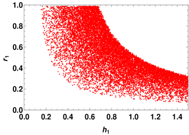
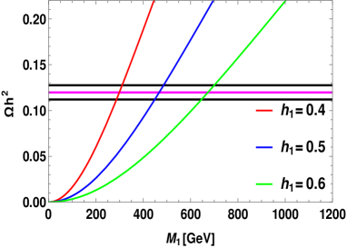
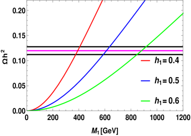
Using the first relation in eqn. (15), we eliminate h2subscriptβ„Ž2h_{2} and since N1subscript𝑁1N_{1} is the lightest odd particle, we take r1<1subscriptπ‘Ÿ11r_{1}<1 suematsu ; vicente2 and |hi|<1.5subscriptβ„Žπ‘–1.5|h_{i}|<1.5 schmidt . Fig. 1 depicts the allowed parameter space (h1,r1)subscriptβ„Ž1subscriptπ‘Ÿ1(h_{1},r_{1}) consistent with current bound on relic abundance planck . Fig. 2 displays the relic abundance as a function of DM mass for various values of h1subscriptβ„Ž1h_{1} at two representative values of r1subscriptπ‘Ÿ1r_{1}, i.e., r1=0.5subscriptπ‘Ÿ10.5r_{1}=0.5 in the left panel and r1=0.6subscriptπ‘Ÿ10.6r_{1}=0.6 in the right panel. This shows that the mass range of DM mass consistent with current relic abundance is proportional with the parameter r1subscriptπ‘Ÿ1r_{1} and the Yukawa coupling h1subscriptβ„Ž1h_{1}.

Refer to caption
Figure 1: Parameter space of h1subscriptβ„Ž1h_{1} and r1subscriptπ‘Ÿ1r_{1} consistent with 3​σ3𝜎3\sigma relic abundance.
Refer to caption
Refer to caption
Figure 2: Variation of relic abundance with DM mass for various values of h1subscriptβ„Ž1h_{1} at r1=0.5subscriptπ‘Ÿ10.5r_{1}=0.5 (left panel) and r1=0.6subscriptπ‘Ÿ10.6r_{1}=0.6 (right panel) where the horizontal line (Magenta) represents the central value of the relic density whereas the black lines denote their corresponding 3ΟƒπœŽ\sigma range.

As the light neutrinos oscillate in flavor, one loop diagrams contribute to lepton flavor violating decays. We now further constrain the parameter space of the model using these decays.

V Lepton flavour violating decays

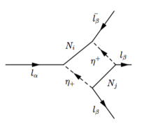
The observation of neutrino oscillations has provided unambiguous signal for lepton number violation in the neutral lepton sector, even though the individual lepton number is conserved in the SM of the electroweak interaction. The evidence of light neutrino masses and mixing and the violation of family lepton number could in principle allow flavor changing neutral current (FCNC) transitions in the charged lepton sector as well, such as ℓα→ℓβ​γ→subscriptℓ𝛼subscriptℓ𝛽𝛾\ell_{\alpha}\to\ell_{\beta}\gamma and ℓα→ℓβ​ℓβ¯​ℓβ→subscriptℓ𝛼subscriptℓ𝛽¯subscriptℓ𝛽subscriptℓ𝛽\ell_{\alpha}\to\ell_{\beta}\overline{\ell_{\beta}}\ell_{\beta}.

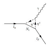
The expression for the branching ratio of lepton flavor violating decay process ℓα→ℓβ​γ→subscriptℓ𝛼subscriptℓ𝛽𝛾\ell_{\alpha}\to\ell_{\beta}\gamma written in terms of dipole form factor ADsubscript𝐴𝐷A_{D} is given by vicente1

Br​(ℓα→ℓβ​γ)=3​(4​π)3​αem4​GF2​|AD|2​Br​(ℓα→ℓβ​να​νβ¯),Brβ†’subscriptℓ𝛼subscriptℓ𝛽𝛾3superscript4πœ‹3subscript𝛼em4superscriptsubscript𝐺𝐹2superscriptsubscript𝐴𝐷2Brβ†’subscriptℓ𝛼subscriptℓ𝛽subscriptπœˆπ›ΌΒ―subscriptπœˆπ›½\mathrm{Br}(\ell_{\alpha}\to\ell_{\beta}\gamma)=\frac{3(4\pi)^{3}\alpha_{\mathrm{em}}}{4G_{F}^{2}}|A_{D}|^{2}\mathrm{Br}\left(\ell_{\alpha}\to\ell_{\beta}\nu_{\alpha}\overline{\nu_{\beta}}\right), (22)

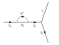
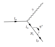
where Ξ±em=e2/4​πsubscript𝛼emsuperscript𝑒24πœ‹\alpha_{\mathrm{em}}=e^{2}/4\pi is the electromagnetic fine structure constant, GFsubscript𝐺𝐹G_{F} is the Fermi constant and α​(Ξ²)𝛼𝛽\alpha(\beta) represents the lepton flavor. The diagrams contributing to ADsubscript𝐴𝐷A_{D} are shown in Fig. 3 and the expression is given by
Refer to caption
Refer to caption
Refer to caption
Figure 3: Diagrams contributing to lΞ±β†’lβ​γ→subscript𝑙𝛼subscript𝑙𝛽𝛾l_{\alpha}\to l_{\beta}\gamma.
AD=βˆ‘i=13hiβ€‹Ξ²βˆ—β€‹hi​α2​(4​π)2​1m02​F2​(ri).subscript𝐴𝐷superscriptsubscript𝑖13superscriptsubscriptβ„Žπ‘–π›½subscriptβ„Žπ‘–π›Ό2superscript4πœ‹21superscriptsubscriptπ‘š02subscript𝐹2subscriptπ‘Ÿπ‘–A_{D}=\sum_{i=1}^{3}\frac{h_{i\beta}^{*}h_{i\alpha}}{2(4\pi)^{2}}\frac{1}{m_{0}^{2}}F_{2}\left(r_{i}\right). (23)

Here expression for the loop function F2​(x)subscript𝐹2π‘₯F_{2}(x) is given in appendix A and for simplicity we consider Ξ»4β‰ͺΞ»3much-less-thansubscriptπœ†4subscriptπœ†3\lambda_{4}\ll\lambda_{3}, thus we get Ξ·+superscriptπœ‚\eta^{+} and Ξ·0superscriptπœ‚0\eta^{0} to be degenerate suematsu . Applying the flavour structure (13), the relation (22) becomes

Br​(ΞΌβ†’e​γ)=3​αem64​π​GF2​m04​|(h22βˆ’0.68​h12)​F2​(r1)+(3.56​h32)​F2​(r3)|2.Brβ†’πœ‡π‘’π›Ύ3subscript𝛼em64πœ‹superscriptsubscript𝐺𝐹2superscriptsubscriptπ‘š04superscriptsuperscriptsubscriptβ„Ž220.68superscriptsubscriptβ„Ž12subscript𝐹2subscriptπ‘Ÿ13.56superscriptsubscriptβ„Ž32subscript𝐹2subscriptπ‘Ÿ32\mathrm{Br}(\mu\to e\gamma)=\frac{3\alpha_{\mathrm{em}}}{64\pi G_{F}^{2}m_{0}^{4}}\left|\left(h_{2}^{2}-0.68h_{1}^{2}\right)F_{2}\left(r_{1}\right)+(3.56h_{3}^{2})F_{2}\left(r_{3}\right)\right|^{2}. (24)

We consider r3>1subscriptπ‘Ÿ31r_{3}>1, M1<2​TeVsubscript𝑀12TeVM_{1}<2{~{}\rm TeV} and M3,m0<8​TeVsubscript𝑀3subscriptπ‘š08TeVM_{3},m_{0}<8{~{}\rm TeV} and thus we work in the mass regime M1≃M2<m0<M3similar-to-or-equalssubscript𝑀1subscript𝑀2subscriptπ‘š0subscript𝑀3M_{1}\simeq M_{2}<m_{0}<M_{3}. Of all the lepton flavor violating (LFV) decays, the decay channel ΞΌβ†’eβ€‹Ξ³β†’πœ‡π‘’π›Ύ\mu\to e\gamma provides most stringent constraint on the parameter space of this model.
Refer to caption
Refer to caption
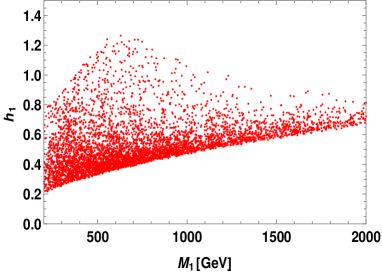
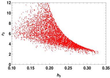
Figure 4: Parameter space of h3subscriptβ„Ž3h_{3} and r3subscriptπ‘Ÿ3r_{3} (left panel) and variation of h1subscriptβ„Ž1h_{1} with M1subscript𝑀1M_{1} (right panel) consistent with neutrino oscillation data, relic density and Br(ΞΌβ†’e​γ)β†’πœ‡π‘’π›Ύ(\mu\to e\gamma).

Imposing the constraints from neutrino mass square differences, relic abundance and current upper bound on Br​(ΞΌβ†’e​γ)Brβ†’πœ‡π‘’π›Ύ{\rm Br}(\mu\to e\gamma) pdg , Fig. 4 (left panel) shows the allowed region in (h3subscriptβ„Ž3h_{3}, r3subscriptπ‘Ÿ3r_{3}) parameter space of the model. From the figure, one can conclude that the lower bound on r3subscriptπ‘Ÿ3r_{3} is 2 (i.e., r3>2subscriptπ‘Ÿ32r_{3}>2) and the upper bound on h3subscriptβ„Ž3h_{3} is 0.33 (i.e., h3<0.33subscriptβ„Ž30.33h_{3}<0.33 ). Fig. 4 (right panel) depicts the variation of h1subscriptβ„Ž1h_{1} with the mass of DM. It shows that Br(ΞΌβ†’e​γ)β†’πœ‡π‘’π›Ύ(\mu\to e\gamma) excludes the values above 1.21.21.2 for h1subscriptβ„Ž1h_{1}. Now taking all the constraints from the flavor and dark sector, one can tabulate the allowed parameter space shown in Table. II.

Parameters Range
r1subscriptπ‘Ÿ1r_{1} Β  0.2β†’1β†’0.210.2\to 1
r3subscriptπ‘Ÿ3r_{3} Β  2β†’12β†’2122\to 12
|h1|subscriptβ„Ž1|h_{1}| Β  0.2β†’1.2β†’0.21.20.2\to 1.2
|h2|subscriptβ„Ž2|h_{2}| Β  0.2β†’1.0β†’0.21.00.2\to 1.0
|h3|subscriptβ„Ž3|h_{3}| Β  0.1β†’0.33β†’0.10.330.1\to 0.33
Table 2: Scotogenic model parameters with their range.

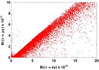
We follow the similar procedure to compute the branching ratios of Ο„β†’eβ€‹Ξ³β†’πœπ‘’π›Ύ\tau\to e\gamma and Ο„β†’ΞΌβ€‹Ξ³β†’πœπœ‡π›Ύ\tau\to\mu\gamma decays. Using the allowed parameter space given in Table-II, we show in Fig. 5 the correlation plot between Br​(Ο„β†’e​γ)Brβ†’πœe𝛾\rm{Br}(\tau\to e\gamma) and Br​(τ→μ​γ)Brβ†’πœπœ‡π›Ύ\rm{Br}(\tau\to\mu\gamma). In our analysis, we have used the measured branching ratios for μ→νμ​e​ν¯eβ†’πœ‡subscriptπœˆπœ‡π‘’subscriptΒ―πœˆπ‘’\mu\to\nu_{\mu}e\bar{\nu}_{e}, Ο„βˆ’β†’Ξ½Ο„β€‹ΞΌβˆ’β€‹Ξ½Β―ΞΌβ†’superscript𝜏subscript𝜈𝜏superscriptπœ‡subscriptΒ―πœˆπœ‡\tau^{-}\to\nu_{\tau}\mu^{-}\bar{\nu}_{\mu} and Ο„βˆ’β†’Ξ½Ο„β€‹eβˆ’β€‹Ξ½Β―eβ†’superscript𝜏subscript𝜈𝜏superscript𝑒subscriptΒ―πœˆπ‘’\tau^{-}\to\nu_{\tau}e^{-}\bar{\nu}_{e} processes from pdg as

Br​(μ→νμ​e​ν¯e)Brβ†’πœ‡subscriptπœˆπœ‡π‘’subscriptΒ―πœˆπ‘’\displaystyle{\rm Br}(\mu\to\nu_{\mu}e\bar{\nu}_{e}) =\displaystyle= 100%,percent100\displaystyle 100\%\;,
Br​(τ→ντ​μ​ν¯μ)Brβ†’πœsubscriptπœˆπœπœ‡subscriptΒ―πœˆπœ‡\displaystyle{\rm Br}(\tau\to\nu_{\tau}\mu\bar{\nu}_{\mu}) =\displaystyle= (17.41Β±0.04)%,percentplus-or-minus17.410.04\displaystyle(17.41\pm 0.04)\%\;,
Br​(τ→ντ​e​ν¯e)Brβ†’πœsubscriptπœˆπœπ‘’subscriptΒ―πœˆπ‘’\displaystyle{\rm Br}(\tau\to\nu_{\tau}e\bar{\nu}_{e}) =\displaystyle= (17.83Β±0.04)%.percentplus-or-minus17.830.04\displaystyle(17.83\pm 0.04)\%\;. (25)
Refer to caption
Figure 5: Correlation plot between Br​(Ο„β†’e​γ)Brβ†’πœe𝛾\rm{Br}(\tau\to e\gamma) and Br​(τ→μ​γ)Brβ†’πœπœ‡π›Ύ\rm{Br}(\tau\to\mu\gamma)

Now we study lepton flavor violation in 3-body decays. As discussed in Ref.vicente1 , these decays get contributions from three types of loop diagrams namely : γ𝛾\gamma-penguin, Z𝑍Z-penguin and box diagrams. The branching ratio for β„“Ξ±β†’3​ℓβ→subscriptℓ𝛼3subscriptℓ𝛽\ell_{\alpha}\to 3\,\ell_{\beta} in scotogenic model is given by vicente1

Br​(ℓα→ℓβ​ℓβ¯​ℓβ)Brβ†’subscriptℓ𝛼subscriptℓ𝛽¯subscriptℓ𝛽subscriptℓ𝛽\displaystyle\text{Br}\left(\ell_{\alpha}\to\ell_{\beta}\overline{\ell_{\beta}}\ell_{\beta}\right) =\displaystyle= 3​(4​π)2​αem28​GF2[|AN​D|2+|AD|2(163log(mΞ±mΞ²)βˆ’223)+16|B|2\displaystyle\frac{3(4\pi)^{2}\alpha_{\mathrm{em}}^{2}}{8G_{F}^{2}}\left[|A_{ND}|^{2}+|A_{D}|^{2}\left(\frac{16}{3}\log\left(\frac{m_{\alpha}}{m_{\beta}}\right)-\frac{22}{3}\right)+\frac{1}{6}|B|^{2}\right. (26)
+(βˆ’2AN​DADβˆ—+13AN​DBβˆ—βˆ’23ADBβˆ—+h.c.)]\displaystyle\left.+\left(-2A_{ND}A_{D}^{*}+\frac{1}{3}A_{ND}B^{*}-\frac{2}{3}A_{D}B^{*}+\mathrm{h.c.}\right)\right]
Γ—Br​(ℓα→ℓβ​να​νβ¯).absentBrβ†’subscriptℓ𝛼subscriptℓ𝛽subscriptπœˆπ›ΌΒ―subscriptπœˆπ›½\displaystyle\times\,\mathrm{Br}\left(\ell_{\alpha}\to\ell_{\beta}\nu_{\alpha}\overline{\nu_{\beta}}\right)\,.
Refer to caption
Figure 6: Penguin diagram contributions to β„“Ξ±β†’3​ℓβ→subscriptℓ𝛼3subscriptℓ𝛽\ell_{\alpha}\to 3\,\ell_{\beta} with the mediator (wavy line) denotes either a photon or a Z-boson.

The coefficient ADsubscript𝐴𝐷A_{D} denotes photon dipole contributions given in eqn. (23), whereas the coefficient AN​Dsubscript𝐴𝑁𝐷{A_{ND}} represents the form factor with the photonic non-dipole contributions given by

AN​D=βˆ‘i=13hiβ€‹Ξ²βˆ—β€‹hi​α6​(4​π)2​1m02​G2​(ri).subscript𝐴𝑁𝐷superscriptsubscript𝑖13superscriptsubscriptβ„Žπ‘–π›½subscriptβ„Žπ‘–π›Ό6superscript4πœ‹21superscriptsubscriptπ‘š02subscript𝐺2subscriptπ‘Ÿπ‘–A_{ND}=\sum_{i=1}^{3}\frac{h_{i\beta}^{*}h_{i\alpha}}{6(4\pi)^{2}}\frac{1}{m_{0}^{2}}G_{2}\left(r_{i}\right). (27)

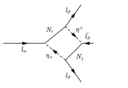
Here G2​(x)subscript𝐺2π‘₯G_{2}(x) is a loop function is given in appendix A. Z𝑍Z-pengiun diagrams shown in Fig. 6 give negligible contribution to the decay width as explained in vicente1 ; vicente2 . Apart from photon dipole and non-dipole penguin contributions, the box diagrams shown in Fig. 7 also contribute to the decay width given by

B=1(4​π)2​e2​m02βˆ‘i,j=13[12D1(ri,rj)hjβ€‹Ξ²βˆ—hj​βhiβ€‹Ξ²βˆ—hi​α+rirjD2(ri,rj))hjβ€‹Ξ²βˆ—hjβ€‹Ξ²βˆ—hi​βhi​α].\displaystyle B=\frac{1}{(4\pi)^{2}{e^{2}}m_{0}^{2}}\sum_{i,\>j=1}^{3}\left[\frac{1}{2}D_{1}(r_{i},r_{j})h_{j\beta}^{*}h_{j\beta}h_{i\beta}^{*}h_{i\alpha}+r_{i}r_{j}D_{2}(r_{i},r_{j}))h_{j\beta}^{*}h_{j\beta}^{*}h_{i\beta}h_{i\alpha}\right]. (28)

The loop functions D1​(x,y)subscript𝐷1π‘₯𝑦D_{1}(x,y) and D2​(x,y)subscript𝐷2π‘₯𝑦D_{2}(x,y) are provided in appendix A.

Refer to caption
Refer to caption
Figure 7: Box diagram contributions to β„“Ξ±β†’3​ℓβ→subscriptℓ𝛼3subscriptℓ𝛽\ell_{\alpha}\to 3\,\ell_{\beta}.

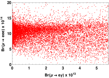
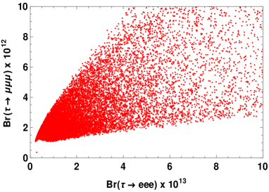
Using the allowed parameter space from Table- II, we show in Fig. 8 the correlation plot between ΞΌβ†’eβ€‹Ξ³β†’πœ‡π‘’π›Ύ\mu\to e\gamma and ΞΌβ†’e​e​eβ†’πœ‡π‘’π‘’π‘’\mu\to eee (left panel). Similarly the right panel in Fig. 8 depicts the correlation plot between branching ratios of Ο„β†’e​e​eβ†’πœπ‘’π‘’π‘’\tau\to eee and Ο„β†’ΞΌβ€‹ΞΌβ€‹ΞΌβ†’πœπœ‡πœ‡πœ‡\tau\to\mu\mu\mu. From these figures we conclude that all the obtained branching ratios in the viable parameter space are within the experimental limits.
Refer to caption
Refer to caption
Figure 8: Correlation plot between Br​(ΞΌβ†’e​e​e)Brβ†’πœ‡π‘’π‘’π‘’{\rm Br}(\mu\to eee) and Br​(ΞΌβ†’e​γ)Brβ†’πœ‡π‘’π›Ύ{\rm Br}(\mu\to e\gamma) (left panel) and between Br​(τ→μ​μ​μ)Brβ†’πœπœ‡πœ‡πœ‡{\rm Br}(\tau\to\mu\mu\mu) and Br​(Ο„β†’e​e​e)Brβ†’πœπ‘’π‘’π‘’{\rm Br}(\tau\to eee) (right panel)

VI Summary and Conclusion

To summarize, in this paper we have considered scotogenic model which is an extension of standard model with an additional inert scalar doublet and three heavy Majorana right-handed neutrinos. It is a noval scenario connecting neutrino physics and dark matter. We have diagonalized the neutrino radiative mass matrix using the TBM matrix with an additional perturbed matrix as a rotation matrix in 13 plane. The mixing angles are chosen (ΞΈ=35βˆ˜πœƒsuperscript35\theta=35^{\circ} and Ο†=12βˆ˜πœ‘superscript12\varphi=12^{\circ}) to accommodate sizeable ΞΈ13subscriptπœƒ13\theta_{13}. Working in a degenerate heavy neutrino mass spectrum, we have obtained the flavor structure favourable to explain normal neutrino mass ordering. Choosing the lightest among the odd particles as dark matter, we have computed the relic abundance including the coannihilation effects. Scanning over the entire parameter space and applying the constraints from neutrino oscillation data, dark matter observables and bounds from lepton flavor violating decays such as ℓα→ℓβ​γ→subscriptℓ𝛼subscriptℓ𝛽𝛾\ell_{\alpha}\to\ell_{\beta}\gamma and β„“Ξ±β†’3​ℓβ→subscriptℓ𝛼3subscriptℓ𝛽\ell_{\alpha}\to 3\,\ell_{\beta}, we have shown the suitable range for various parameters in the model.

Appendix A Loop functions

The loop functions used in LFV decays are given by

F2​(x)subscript𝐹2π‘₯\displaystyle F_{2}(x) =\displaystyle= 1βˆ’6​x2+3​x4+2​x6βˆ’6​x4​log⁑x26​(1βˆ’x2)4,16superscriptπ‘₯23superscriptπ‘₯42superscriptπ‘₯66superscriptπ‘₯4superscriptπ‘₯26superscript1superscriptπ‘₯24\displaystyle\frac{1-6x^{2}+3x^{4}+2x^{6}-6x^{4}\log x^{2}}{6(1-x^{2})^{4}}, (29)
G2​(x)subscript𝐺2π‘₯\displaystyle G_{2}(x) =\displaystyle= 2βˆ’9​x2+18​x4βˆ’11​x6+6​x6​log⁑x26​(1βˆ’x2)4,29superscriptπ‘₯218superscriptπ‘₯411superscriptπ‘₯66superscriptπ‘₯6superscriptπ‘₯26superscript1superscriptπ‘₯24\displaystyle\frac{2-9x^{2}+18x^{4}-11x^{6}+6x^{6}\log x^{2}}{6(1-x^{2})^{4}}, (30)
D1​(x,y)subscript𝐷1π‘₯𝑦\displaystyle D_{1}(x,y) =\displaystyle= βˆ’1(1βˆ’x2)​(1βˆ’y2)βˆ’x4​log⁑x2(1βˆ’x2)2​(x2βˆ’y2)βˆ’y4​log⁑y2(1βˆ’y2)2​(y2βˆ’x2),11superscriptπ‘₯21superscript𝑦2superscriptπ‘₯4superscriptπ‘₯2superscript1superscriptπ‘₯22superscriptπ‘₯2superscript𝑦2superscript𝑦4superscript𝑦2superscript1superscript𝑦22superscript𝑦2superscriptπ‘₯2\displaystyle-\frac{1}{(1-x^{2})(1-y^{2})}-\frac{x^{4}\log x^{2}}{(1-x^{2})^{2}(x^{2}-y^{2})}-\frac{y^{4}\log y^{2}}{(1-y^{2})^{2}(y^{2}-x^{2})}, (31)
D2​(x,y)subscript𝐷2π‘₯𝑦\displaystyle D_{2}(x,y) =\displaystyle= βˆ’1(1βˆ’x2)​(1βˆ’y2)βˆ’x2​log⁑x2(1βˆ’x2)2​(x2βˆ’y2)βˆ’y2​log⁑y2(1βˆ’y2)2​(y2βˆ’x2).11superscriptπ‘₯21superscript𝑦2superscriptπ‘₯2superscriptπ‘₯2superscript1superscriptπ‘₯22superscriptπ‘₯2superscript𝑦2superscript𝑦2superscript𝑦2superscript1superscript𝑦22superscript𝑦2superscriptπ‘₯2\displaystyle-\frac{1}{(1-x^{2})(1-y^{2})}-\frac{x^{2}\log x^{2}}{(1-x^{2})^{2}(x^{2}-y^{2})}-\frac{y^{2}\log y^{2}}{(1-y^{2})^{2}(y^{2}-x^{2})}. (32)

In the limit yβ†’x→𝑦π‘₯y\to x, the functions D1subscript𝐷1D_{1} and D2subscript𝐷2D_{2} become

D1​(x,x)=βˆ’1+x4βˆ’2​x2​log⁑x2(1βˆ’x2)3,subscript𝐷1π‘₯π‘₯1superscriptπ‘₯42superscriptπ‘₯2superscriptπ‘₯2superscript1superscriptπ‘₯23\displaystyle D_{1}(x,x)=\frac{-1+x^{4}-2x^{2}\log{x^{2}}}{(1-x^{2})^{3}}, (33)
D2​(x,x)=βˆ’2+2​x2βˆ’(1+x2)​log⁑x2(1βˆ’x2)3.subscript𝐷2π‘₯π‘₯22superscriptπ‘₯21superscriptπ‘₯2superscriptπ‘₯2superscript1superscriptπ‘₯23\displaystyle D_{2}(x,x)=\frac{-2+2x^{2}-(1+x^{2})\log{x^{2}}}{(1-x^{2})^{3}}. (34)

References

  • (1) P.Β Minkowski, Phys. Lett. B, 67: 421 (1977); R. N.Β Mohapatra and G.Β Senjanovic, Phys. Rev. Lett. 44: 912 (1980); M.Β Gell-Mann, P.Β Ramond, and R.Β Slansky (1980), print-80-0576 (CERN); J.Β Schechter and J. W. F.Β Valle, Phys. Rev. D, 22: 2227 (1980).
  • (2) R. N. Mohapatra and G. Senjanovic, Phys. Rev. D, 23: 165 (1981); G. Lazarides, Q. Shafi and C. Wetterich, Nucl. Phys. B, 181: 287 (1981); C. Wetterich, Nucl. Phys. B, 187: 343 (1981); B. Brahmachari and R. N. Mohapatra, Phys. Rev. D, 58: 015001 (1998); S. Antusch and S. F. King, Phys. Lett. B, 597: 199 (2004); R. N. Mohapatra, Nucl. Phys. Proc. suppl. 138: 257 (2005).
  • (3) R. Foot, H. Lew, X. G. He et al, Z. Phys. C, 44: 441 (1989).
  • (4) E.Β Ma, Phys. Rev. D, 73: 077301 (2006), arXiv:hep-ph/0601225.
  • (5) B. Pontecorvo, Sov. Phys. JETP, 7: 172 (1958); Z. Maki, M. Nakagawa and S. Sakata, Prog. Theor. Phys, 28: 870 (1962).
  • (6) F.Β P.Β An et al (DAYA-BAY Collaboration), Phys. Rev. Lett. 108: 171803 (2012), arXiv:1203.1669.
  • (7) F.Β P.Β An et al (DAYA-BAY Collaboration), Chin. Phys. C, 37: 011001 (2013), arXiv:1210.6327.
  • (8) J.Β K.Β Ahn et al (RENO Collaboration), Phys. Rev. Lett. 108: 191802 (2012), arXiv:1204.0626.
  • (9) K.Β Abe et al (T2K Collaboration), Phys. Rev. D, 88: 032002 (2013), arXiv:1304.0841.
  • (10) D.Β Forero, M.Β Tortela and J.Β Valle, Phys. Rev. D, 90: 093006 (2014), arXiv:1405.7540.
  • (11) P. A. R. Ade et al (Planck Collaboration), Astron. Astrophys. 571: A1 (2014), arXiv:1303.5062.
  • (12) L.Β LepozΒ Honorez, E.Nezri, J.Β F.Β Oliver et al, JCAP, 02: 28 (2007), arXiv:hep-ph/0612275.
  • (13) R.Β Barbieri, L.Β E.Β Hall and V.Β S.Β Rychkov, Phys. Rev. D, 74: 015007 (2006), arXiv:hep-ph/0603188.
  • (14) M. Gustafsson, PoS CHARGED, 2010: 030 (2010), arXiv:1106.1719.
  • (15) Daijiro Suematsu, Takashi Toma, Tetsuro Yoshida, Phys. Rev. D, 79: 093004 (2009), arXiv:0903.0287.
  • (16) D. Schmidt, T Schwetz, T. Toma, Phys. Rev. D, 85: 073009 (2012), arXiv:1201.0906.
  • (17) T. Toma and A. Vicente, JHEP, 01: 160 (2014), arXiv:1312.2840.
  • (18) A. Vicente, C E. Yaguna, JHEP, 02: 144 (2015), arXiv:1412.2545.
  • (19) G. Altarelli, F. Ferugilo, Rev. Mod. Phys. 82: 2701 (2010); G. Altarelli, F. Ferugilo, L. Merlo, E. Stamou, JHEP, 08: 021 (2012), arXiv:1205.4670; S. F. King and C. Luhn, Rept. Prog. Phys. 76: 056201 (2013), arXiv:1301.1340; S. F. King, A. Merle, S. Morisi et al, New Journ. Phys. 16: 045018 (2014); H. Isimori et al., Prog. Theor. Phys. Suppl. 183: 1 (2010).
  • (20) P. F. Harrison, D. H. Perkins, and W.G. Scott, Phys. Lett. B, 458: 79 (1999); Phys. Lett. B, 530: 167 (2002); Z. Z. Xing, Phys. Lett. B, 533: 85 (2002); P. F. Harrison and W. G. Scott, Phys. Lett. B, 535: 163 (2002); Phys. Lett. B, 557: 76 (2003); X.-G. He and A. Zee, Phys. Lett. B, 560: 87 (2003); L. Wolfenstein, Phys. Rev. D, 18: 958 (1978); Y. Yamanaka, H. Sugawara, and S. Pakvasa, Phys. Rev. D, 25: 1895 (1982); D, 29: 2135(E) (1984); N. Li and B.-Q. Ma, Phys. Rev. D, 71: 017302 (2005), arXiv:hep-ph/0412126.
  • (21) M. Sruthilaya, C. Soumya, K.N. Deepthi et al, New J. Phys. 17: 083028 (2015), arXiv:1408.4392.
  • (22) K.Β Griest and D.Β Seckel, Phys. Rev. D, 43: 3191 (1991).
  • (23) K. A. Olive et al, Particle Data Group Collaboration, Chin. Phys. C, 38: 090001 (2014).