Detection of a very low mass star in an Eclipsing Binary system

Abstract

We report the detection of a very low mass star (VLMS) companion to the primary star 1SWASPJ234318.41$+$295556.5A (J2343$+$29A), using radial velocity (RV) measurements from the PARAS (PRL Advanced Radial-velocity Abu-sky Search) high resolution echelle spectrograph. The periodicity of the single-lined eclipsing binary (SB₁) system, as determined from 20 sets of RV observations from PARAS and 6 supporting sets of observations from SOPHIE data, is found to be $16.953$ d as against the $4.24$ d period reported from SuperWasp photometry. It is likely that inadequate phase coverage of the transit with SuperWasp photometry led to the incorrect determination of the period for this system. We derive the spectral properties of the primary star from the observed stellar spectra: $T_{\rm{eff}}$ = 5125$~{}\pm~{}67$ K, $[Fe/H]$ = $0.1~{}\pm~{}0.14$ and ${\rm log}~{}g$ = $4.6~{}\pm~{}0.14$, indicating a K1V primary. Applying the Torres relation to the derived stellar parameters, we estimate a primary mass $0.864_{-0.098}^{+0.097}$ M_⊙ and a radius of $0.854_{-0.060}^{+0.050}$ R_⊙. We combine RV data with SuperWASP photometry to estimate the mass of the secondary, $M_{B}=0.098\pm 0.007M_{\sun}$, and its radius, $R_{B}=0.127\pm 0.007~{}R_{\sun}$, with an accuracy of $\sim$7$\%$. Although the observed radius is found to be consistent with the Baraffe’s theoretical models, the uncertainties on the mass and radius of the secondary reported here are model dependent and should be used with discretion. Here, we establish this system as a potential benchmark for the study of VLMS objects, worthy of both photometric follow-up and the investment of time on high-resolution spectrographs paired with large-aperture telescopes.

1 Introduction

M dwarfs make up most of the galaxy’s stellar budget. However, due to their small masses and fainter magnitudes in the visible band, such systems have remained largely unexplored. The Mass-Radius (M-R) relation serves as a crucial test for the verification of theoretical models of M dwarfs against values derived from observation. This is also integral to the understanding of stellar structure and evolution. Compared to M dwarfs, stars with masses $\geq 0.6M_{\sun}$ have a well-established M-R relation (Torres, Andersen & Giménez, 2010). The vast majority of observations of M dwarfs of varying masses have reported radii higher than those predicted by models (Torres, Andersen & Giménez, 2010; López-Morales, 2007). Improper assumptions of opacity in M dwarf models is speculated to be one of the reasons for this mismatch between observational and theoretically predicted radii of M dwarfs, at the level of $\sim 10-15\%$. Chabrier et al. (2007) argue that the discrepancy is due to the high rotation rate in M dwarfs, or the effect of magnetic-field-induced reduction of the efficiency of large-scale thermal convection in their interior.

M dwarfs having masses of less than $0.3M_{\sun}$ seem to match the Baraffe models (Baraffe et al., 2015) closely, as the stars become completely convective at this boundary (López-Morales, 2007). If we choose to concentrate on very low mass stars (VLMS) $\leq$ $0.1M_{\sun}$, there is a dearth of such samples discovered with accuracies $\leq$ 1–2 $\%$. There have been only a handful of EB systems studied at such high accuracies in which one of the components is VLMS object with mass $\leq$ 0.1 $M_{\odot}$ (Wisniewski et al., 2012; Triaud et al., 2013; Gómez Maqueo Chew et al., 2014; Ofir et al., 2012; Tal-Or et al., 2013; Beatty et al., 2007) where masses of the objects have been determined at high accuracies. Table 1 gives a non-exhaustive compilation of the stars having masses between $0.08-0.4$ M_⊙ for which masses and radii are determined at accuracies better than 10$\%$. The first three columns contain the name of the object, its mass and radius. The systems are SB₁ or SB₂ by nature. The classification of the EB, based on spectral types, is mentioned in the penultimate column. The literature references in which the sources are studied are cited in the last column of the table. A theoretical M-R diagram is plotted in Fig. 1 for the M dwarfs having masses between $0.08-0.4$ M_⊙ based on Baraffe models (Baraffe et al., 2015) for 1 Gyr isochrone and solar metallicity (most of the objects studied here have this age and metallicity). We have overplotted objects studied in literature from Table 1 with their respective error bars on masses and radii on the theoretical M-R diagram. As seen from Fig. 1, many of the stars studied in literature fall above the theoretical M-R plot clearly indicative of the M dwarf radius problem. Moreover, we also see that this discrepancy is more pronounced for objects having masses above 0.3 $M_{\odot}$. Out of 26 systems studied previously in literature, in the mass range of $0.08-0.4$ $M_{\odot}$ as shown in Table 1, there have been only 6 systems having masses between $0.08-0.2$ $M_{\odot}$ studied with accuracies better than a few per cent (Beatty et al., 2007; Doyle et al., 2011; Triaud et al., 2013; Nefs et al., 2013; Fernández et al., 2009). There is thus a greater need for identifying more such VLMS candidates in EB systems and more specifically in the mass range of $0.08-0.4$ $M_{\odot}$ where there are only few sources studied.

The object chosen for the current study, J2343$+$29A, was first identified from SuperWasp (SW) photometry by Christian et al. (2006) and Collier Cameron et al. (2007). Observations taken from the SW North listed the primary star, J2343$+$29A, having a temperature of 5034 K, spectral type K3, a radius of ${R_{A}=~{}0.85~{}R_{\sun}}$ and a transit depth of 21 mmag. The transit light curve showed substantial scatter, and source was suspected to be a stellar binary system as per preliminary observations with SOPHIE (Collier Cameron et al., 2007). Table 2 summarizes the basic stellar parameters listed for this source in the literature (Collier Cameron et al., 2007).

Here, we present the discovery and characterization of a VMLS companion to J2343$+$29A, enabled by the PRL Advanced Radial velocity Abu-sky Search spectrograph (hereafter PARAS; Chakraborty et al., 2014). Spectra acquired using PARAS, over a time period of $\sim$ 3 months and well-sampled in phase, are described in §2. In §3 we describe our radial velocity (RV) analysis, both independently and in concert with SW photometry. We have developed an IDL-based tool PARAS SPEC to determine stellar properties like $T_{\rm{eff}}$, surface gravity (${\rm log}~{}g$), and metallicity ($[Fe/H]$). This procedure, involving matching synthetic spectra with the observed spectra, and fitting the Fe I, Fe II absorption line equivalent width (EW), is discussed in §4. Also discussed in §4 are the stellar parameters of the primary star derived from the observed PARAS spectra. In §5, we discuss the implications of this work, and conclude in §6.

2 RV observations of J2343$+$29 with PARAS

High-resolution spectroscopic observations of the star J2343$+$29A were taken with the fiber-fed echelle spectrograph, PARAS, at the 1.2 m telescope at Gurushikhar Observatory, Mount Abu, India. A set of 20 observations of the source acquired between November 2013 and January 2014 at a resolving power of 67000 were used for determining the orbital fit of the system. Details of the spectrograph, observational procedure, and data analysis techniques can be found in Chakraborty et al. (2014). The spectra were recorded in the simultaneous reference mode with ThAr as the calibration lamp. All nights of observations were spectroscopic in nature. The magnitude of the source in the V band is $\sim$ 10.7, which is the limit of faintness of observations possible with PARAS on the 1.2 m telescope. The exposure time for observations was chosen to be 1800 s such that a signal-to-noise ratio (S/N) between 12–14 pixel^-1 at 5500 Å was obtained for each spectrum. Observations with S/N less than 11.5 pixel^-1 due to poor weather conditions or/and high air mass during observations (Air Mass $\geq$ 1.5), were not considered for orbital fitting. A list of epochs and observational details is shown in Table 3. The first two columns represent the observation time in UT and BJD respectively. The exposure time and observed RV are given in the following columns. The RV error based on photon noise and the uncertainties associated due to the cross correlation function (CCF) fitting are given in the last column (see §3 for details).

3 Results

3.1 The Radial Velocity analysis

The PARAS data analysis pipeline as described in Chakraborty et al. (2014) is custom-designed, fully automated and consists of robust IDL routines, based on the REDUCE routines of Piskunov & Valenti (2002). The pipeline performs the routine tasks of cosmic ray correction, dark subtraction, order tracing, and order extraction. A thorium line list is used to create a weighted mask which calculates the overall instrument drift, based on the simultaneous ThAr exposures. RVs are derived by cross-correlating the target spectra with a suitable numerical stellar template mask. The stellar mask is created from a synthetic spectrum of the star, containing the majority of deep photospheric absorption lines. See (Pepe et al., 2002); and references therein for a more detailed description of the mask cross-correlation method. In this case, we use a K-type stellar mask for cross-correlation. RV measurement errors are based on photon noise errors (Bouchy et al., 2001) and the errors associated with the CCF fitting function. We randomly vary the signal on each pixel within $\pm\sqrt{N}$, where N is the signal on each pixel, and thereafter run the CCF for each spectra. This process is repeated 100 times for each spectra and the standard deviation of the distribution of the obtained RV values gives the 1 $\sigma$ uncertainty on the CCF fitting along with errors from photon noise on each RV point. The barycentric corrected RV values and their respective uncertainties are shown in Table 3.

We combined PARAS observations with available SOPHIE archival data to gain a longer baseline for observations, from August 2006 to January 2014, time span of 7.5 years. We retrieved 6 observations of the star between August 2006 to August 2007 from the SOPHIE archival data . The SOPHIE observations for the source J2343$+$29A were obtained in the High Efficiency (HE) mode of SOPHIE, with a resolving power of $\sim$ 40000 covering the wavelength region 3872-6943 Å. SOPHIE archival data are processed by the standard SOPHIE pipeline and passed through weighted cross-correlation with a numerical mask (Pepe et al., 2002). As per the header information in the retrieved archival data, the S$/$N for each epoch varied between $\sim$25–75 pixel^-1 at 5500 Å. The errors on RV, as given in the header information, were calculated by the semi-empirical estimator $\sigma_{RV}~{}=~{}A~{}\times~{}\sqrt{FWHM}/(S/N~{}\times~{}C)$ as suggested by West et al. (2009) for SOPHIE data where ’A’ is the empirically determined constant and ’C’ is the contrast factor in the spectra. External systematic errors of 2 m s^-1 (spectrograph drift uncertainty) and guiding errors of 4 m s^-1 were added in quadrature (Boisse et al., 2010) to the obtained statistical errors. The RV values from SOPHIE archival data and the errors on each point are given in Table 4.

Using EXOFAST (Eastman, Gaudi & Agol, 2013), we fit the spectroscopy data from the PARAS and SOPHIE spectrographs. EXOFAST is a set of IDL routines designed to fit transit and RV variations simultaneously or separately, and characterize the parameter uncertainties and covariances using the Differential Evolution Markov Chain Monte Carlo method (Johnson et al., 2011). It requires priors on $T_{\rm{eff}}$, ${\rm log}~{}g$ and iron abundance ($[Fe/H]$) as an input for estimating the stellar parameters of the primary star. We provide priors of $T_{\rm{eff}}$ = 5125$~{}\pm~{}67$ K, $[Fe/H]$ = $0.1~{}\pm~{}0.14$, and ${\rm log}~{}g$ = $4.6~{}\pm~{}0.1$ to EXOFAST. These priors are estimated on the basis of detailed spectroscopic analysis performed using the newly developed PARAS SPEC package, as discussed in §4. The RV fitting package EXOFAST uses empirical polynomial relations between masses and radii of stars (for masses $\geq 0.6M_{\sun}$); their ${\rm log}~{}g$, $T_{\rm{eff}}$, and $[Fe/H]$ based on a large sample of non-interacting binary stars, in which all of these parameters were well-measured (Torres, Andersen & Giménez, 2010). These priors are used as a convenient way of modelling isochrones and are fast enough to incorporate them at each step in the Markov chain. The errors are determined by evaluating the posterior probability density, based on the range of a given parameter that encompasses some set fraction of the probability density for the given model. It may be noted here that the RV semi amplitude (K) value as measured with EXOFAST is independent of the modelled stellar parameters and has no bias contingency on any of the masses of primary or secondary stars. K value is further used independent of EXOFAST to derive the mass function $f(m)$ for the EB system which is given by (Kallrath et al., 2000)

$$f(m)=\frac{m_{1}~{}\sin^{3}i}{{(1+q)}^{2}}$$ (1)

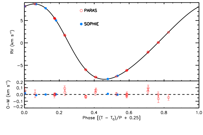
Figure 2: (Top panel) PARAS, Mount Abu (open red circles) and SOPHIE (filled blue circles) observed data points along with the estimated errors are plotted. RV model curve for star 1SWASP J2334318+295556 obtained from EXOFAST is overplotted against orbital phase on the observed data points. The RV model here describes the case of ”RV fit alone” as described in Table 4. (Bottom panel) The residuals from best-fitting are plotted below the RV plot. For better visual representation, the x axis in Phase is shifted by 0.25 so that the central primary transit crossing point (T_c) occurs at phase 0.25 instead of 0. P indicates the period.

Here, $m{{}_{1}}$ and $m{{}_{2}}$ are masses of the two components and q is the mass ratio of the components of EB. A knowledge of the primary mass ($m_{1}$) and $\sin i$ is needed to calculate the secondary mass ($m_{2}$). The former quantity can be derived by priors such as ${\rm log}~{}g$, $T_{\rm{eff}}$, and $[Fe/H]$, which are estimated by high-resolution spectroscopy as discussed in § 4 while the latter one can be derived by photometry as presented in § 3.2. In the singular application of RV fitting, EXOFAST is equally applicable to EBs and star-planet systems. However, EXOFAST uses planet approximation that ignores the mass of the secondary while calculating the orbital separation. This assumption may affect the accuracy of the derived radius of the secondary. RV values were corrected for the offset between the two spectrographs, which amounted to 259 m s^-1. The results of this procedure are summarized in Table 5, in the 3^rd column “RV fit only”. We determine the period of the EB as $16.953$ d with a RV semi-amplitude of $8398$ m s^-1. Fig. 2 illustrates a plot of RV versus orbital phase for J2343$+$29A. Red open circles (top panel) show RV measurements of the primary taken with PARAS, and solid blue circles denote the same for SOPHIE. The solid black curve indicates the best fit model from EXOFAST based on the parameters in Table 5. The bottom panel in Fig. 2 shows the model fit and the residuals (Observed-Model).

We tried fitting the RV data on exactly 4 times the photometry period (16.96 d) but could not constrain the fit. Thus, it should be noted that the observed period is approximately 4 times the reported period of 4.24 d from SW photometry. Since there are sufficient number of RV points, well sampled in phase of the eclipsing binary (EB), we consider the revised period of the EB from RV measurements alone to be accurate.

3.2 SuperWASP photometry

The light curve for J2343$+$29, as seen in Fig. 17 of Christian et al. (2006), shows a moderate amount of scatter and an ellipsoidal amplitude of 2.9, hinting at the possibility of stellar binary (Christian et al., 2006). They identified a period of 4.24 d whereas RV data (this work) shows a periodicity of 16.953 d. The misidentification of the period by SW photometry could be due to the fact that the automated SW pipeline is intended to search for short period planets typically less than 5 d. The probability of finding transits in SW photometry, with periods that are integral multiples of 1 d or 1.5 d, is comparatively low, at around $\sim$ 35$\%$ (Street et al., 2007). Since J2343$+$29 has an RV determined period of 16.953 d (which is much higher than 5 d and also a close integral multiple of 1 d), there is greater likelihood of sampling the source poorly in phase during the entire transit duration. There are 6 transits detected for this source at $\sim$ 4.24 d periodicity as reported in Christian et al. (2006). Due to the relatively low number of recorded transits, the phase coverage of the transit event is expected to be poor.

3.3 Simultaneous spectroscopy and photometry fitting

We fit the RV datasets and light curves simultaneously in order to impose better constraints on the execution of EXOFAST. The results of the execution are summarized in Table 5 in the 4^th column “Combined RV-transit fit”. We determine the period of the EB to be $16.95350\pm 0.00005$ d with a RV semi-amplitude of $8407_{-10}^{+11}$ km s^-1. The orbital separation between the EB components is $0.1271_{-0.0049}^{+0.0066}$ AU. Fig. 3 (upper panel) shows the simultaneous fit for the transit light curve obtained by analysing SW photometry data (filled circles) overplotted with the model derived from EXOFAST (solid curve). The RV plot produced by simultaneous fit of RV and transit data has a close resemblance with Fig. 2. The residuals are plotted in lower panel. The simultaneous fit gives us a transit depth of $0.025\pm 0.001$ mag, angle of inclination of $89.55_{-0.40}^{+0.12}$ and a transit duration of $235\pm 7$ m. Although we see a clear transit dip in the light curve, we notice that there are fewer data points close to the egress of the transit.

4 Spectral analysis

The double-lined EBs (SB₂) enable the most accurate measurements of the radii and masses of the stars. Since in such systems spectra of both the stars can be recorded, RV measurements lead to precise determination of masses of the stars in the system directly. However, in single-lined EBs (SB₁) systems, where the spectra of only the primary source is available, mass of the secondary is deduced by quantifying the amplitude of the wobble of the primary star in the binary system. In order to infer mass of the primary and to classify whether the star is in main-sequence or in giant or sub-giant phase, it is essential to know the surface gravity (g = GM/R²), often quoted in the form of ${\rm log}~{}g$, surface temperature ($T_{\rm{eff}}$), and metallicity ($[Fe/H]$) of the star. A detailed study by Torres, Andersen & Giménez (2010) on a large sample of EBs has led to the establishment of an empirical relation for the mass and radius of the stars above 0.6 M_⊙ based on the stellar parameters, i.e, ${\rm log}~{}g$, the $T_{\rm{eff}}$ and $[Fe/H]$. In our case, since we have high-resolution spectroscopy data obtained for RV measurements, we can use the same data to derive the stellar parameters. There are many host stars like J2343$+$29, for which spectral properties have not been studied. The quantification of these parameters is of utmost importance to draw inferences about their masses and radii. In this context, we have developed a pipeline PARAS SPEC, to estimate the stellar atmospheric parameters from the analysis of stellar spectra. With high-resolution spectroscopy, it is possible to determine $T_{\rm{eff}}$ and $[Fe/H]$ (based on Fe I and Fe II lines) as well as ${\rm log}~{}g$ (based on Mg I lines) at high accuracies. The pipeline, a set of IDL-based tools, is developed to facilitate the determination of stellar properties. The determination of stellar properties from observed PARAS spectra is based on two methods. The first one involves of matching of observed spectra with synthetic spectra. The second method is based on the measurement of EW from a set of Fe I and Fe II lines in the observed spectra (Blanco-Cuaresma et al., 2014). We have developed an IDL-based tool, PARAS SPEC, to facilitate the process of estimation of stellar parameters from observed PARAS spectra. The tool is easy to use, and has the ability to include a variety of stellar atmosphere models, abundances or line lists, depending on the spectral type of the star. We combine the data for different epochs to obtain a higher S/N spectra for this spectral analysis. The steps used by PARAS SPEC are briefly described below.

4.1 Preliminary correction of observed spectra

The simultaneous ThAr mode PARAS spectra obtained for RV are also used for stellar characterization. Though PARAS has a spectral coverage of 3800–9500 Å, we utilize only the ThAr calibrated region of 3800–6800 Å. In this wavelength range, average separation between neighbouring orders is 17 pixels (Chakraborty et al., 2014). Contamination occurs where argon lines are bright enough to spill over the stellar spectra in the neighbouring order. To correct for this, we subtract Dark-ThAr (first fiber is kept dark and the second fiber is illuminated by ThAr) of similar exposure time as that of the star spectra from the star-ThAr file. This greatly mitigates ThAr contamination in the stellar spectrum within the cited uncertainties. PARAS SPEC requires blaze corrected and normalized stellar spectra as input data. For this purpose, a polynomial function is fitted iteratively to an accuracy of $\sim$1 $\%$ across the stellar continuum blaze profile, ignoring absorption features in the stellar spectra for each order. The observed spectrum is then divided by the polynomial function to blaze correct and normalize it at a given epoch. All observed epochs are then co-added in velocity space to improve the S/N of the stellar spectrum. All the orders are combined and stitched to a single spectra based on S/N of the spectra. The overlapping regions are combined at the mid-point while stitching the orders.

4.2 Generation of synthetic library

Synthetic spectra generator code SPECTRUM (Gray et al., 1999)  utilizes the Kurucz models (Kurucz, 1993) for stellar atmosphere parameters. SPECTRUM works on the principle of local thermodynamic equilibrium and plane parallel atmospheres. It is suitable for generation of synthetic spectra for stars from B to mid M type. It is developed with C compiler environment with a terminal mode interface to access it. We resampled the synthetic spectra at the PARAS resolving power of $67000$. We first worked with the solar spectrum observed (at a $S/N$ $\sim$150) with PARAS in order to adjust various parameters for the library of synthetic spectra, such as, microturbulence ($v_{\rm{micro}}$), macroturbulence ($v_{\rm{macro}}$), rotational velocity ($v\sin i$), $T_{\rm{eff}}$, $[Fe/H]$ and ${\rm log}~{}g$. When all the parameters are kept free, the best-derived model having the least $\chi^{2}$ for the PARAS observed solar spectra has the following values for various parameters: $v_{\rm{micro}}$ = 0.85 km s^-1 and $v_{\rm{macro}}$ = 2 km s^-1. The value for $v_{\rm{micro}}$ obtained here is in close agreement with the one derived by Blackwell et al. (1984). The value of $v_{\rm{macro}}$ = 2 km s^-1 derived here is consistent with the value of 2.18 km s^-1 obtained by (Valenti & Piskunov, 1996). A library of $19,200$ synthetic spectra are generated based on different combinations of $T_{\rm{eff}}$, $[Fe/H]$, ${\rm log}~{}g$, and $v\sin i$. The generated synthetic library consists of a coarse grid that was interpolated on-the-fly while running iterations, in an effort to increase the precision of derived parameters. The library ranges in $T_{\rm{eff}}$ between $4000-7000$ K at a temperature interval of $250$ K, in $[Fe/H]$ between $-2.5-0.5$ dex with an interval of $0.5$, in ${\rm log}~{}g$ between $3.0-5.0$ dex at an interval of $0.5$ and $vsini$ between $1-40$ km s^-1 at $1$ km s^-1 interval. The wavelength ranges between $5050-6560$ Å at $0.01$ Å interval.

4.3 Methodology for spectral analysis

As mentioned earlier, EXOFAST requires priors such as ${\rm log}~{}g$, the $T_{\rm{eff}}$ and $[Fe/H]$. In order to obtain these, we analysed the spectra using two methods described below.

4.3.1 Synthetic Spectral Fitting

In this method, the observed spectrum is matched with a library of synthetic spectra given as mentioned in § 4.2 after adjusting for the instrument resolution. The spectrum having the best match (minimum $\chi^{2}$ value) gives the best-fit result for the spectral properties of the star. We carefully adjusted the continua by comparing observed PARAS spectra with synthetic spectra. The wavelength region of $5050-6500~{}\AA$ is used for this exercise, and the RMS residual $\sum\nolimits{(O(i)-M(i))}^{2}$ is computed. $T_{\rm{eff}}$, $[Fe/H]$ and $v\sin i$ are simultaneously determined from the entire wavelength region whereas ${\rm log}~{}g$ is determined from the Mg lines within $5160-5190~{}\AA$, after fixing $T_{\rm{eff}}$, $[Fe/H]$ and $v\sin i$ from the previous step. This method requires a minimum S/N of $\sim 80$ pixel^-1 in the entire wavelength region covered. For fainter stars, we concentrate on red end between $6000-6500~{}\AA$ of the CCD where S/N is mostly above 80 (for stars upto 11 magnitude in V band having sufficient number of epochs co-added).

4.3.2 Equivalent Width Method (EW)

The EW method works on the principle of inducing neutral and ionized iron lines to invoke excitation equilibrium and ionization balance. Here, abundances as a function of excitation potential should have no trends. Abundances as a function of reduced EW (EW/$\lambda$) should exhibit no trends and the abundances of neutral iron (Fe I) and ionized iron (Fe II) should be balanced (Blanco-Cuaresma et al., 2014). A model which satisfies the above mentioned criteria is the best-fit model as determined by this method. We measure the EW of a set of Fe I and Fe II lines from the line list of Sousa et al. (2014). Each line is carefully inspected visually for line blends before abundances are determined through EW measurements by using SPECTRUM. After careful inspection of the EW fits as discussed above, a set of EW of the fitted lines is given as an input to the ABUNDANCE subroutine of SPECTRUM. The subroutine uses various stellar models which are formed as a combination of different $T\rm{{}_{eff}}$, $[Fe/H]$, ${\rm log}~{}g$ and $v_{\rm{micro}}$ as given in § 4.2. With the above mentioned inputs, SPECTRUM is able to compute abundance of each Fe I or Fe II line. $[Fe/H]$ is kept fixed for EW analysis, to a value previously determined through literature or by the synthetic spectral fitting method. $[Fe/H]$ and v_micro are degenerate (Valenti & Fischer, 2005) and thereby both the parameters cannot be kept free simultaneously. For the EW method, we fix $[Fe/H]$ to determine v_micro independently. Apart from the central value of $[Fe/H]$, two more iterations are executed on $\pm\sigma$ value of $[Fe/H]$, thereby error on each parameter is determined. Thus, the set of parameters where the slopes and the difference are simultaneously minimized give us the best-determined $T_{\rm{eff}}$, v_micro) and ${\rm log}~{}g$.

4.3.3 Uncertainties and limitations of the method

The synthetic spectral fitting method yields reliable results only for spectra having S/N per pixel $\geqslant$ 80. Between S/N $80-100$, the wavelength region of $6000-6500~{}\AA$ can be used for stellar property estimation. However, we lose information on ${\rm log}~{}g$ which is determined by Mg I lines ($5160-5190~{}\AA$). For such cases, the EW method which works for spectra having S/N per pixel $\geqslant$ 50 can be used to determine stellar properties. For, S/N $\geqslant$ 100, both the methods work well to determine all three stellar parameters, $T\rm{{}_{eff}}$, $[Fe/H]$ and ${\rm log}~{}g$. If the S/N per pixel at 6000 Å is above 120, the uncertainities in $T\rm{{}_{eff}}$ and ${\rm log}~{}g$ are $\pm 25$ K and $\pm 0.05$ respectively for both the methods. For S/N per pixel (at 6000 Å ) between 80–100, the uncertainties are $\pm 50$ K and $\pm 0.1$ respectively. Similar numbers for S/N per pixel between 50–80 are $\pm 100$ K and $\pm 0.1$. Apart from these uncertainties, there could be systematic errors introduced for each of the methods. Detailed systematic error analysis for these methods is beyond the scope of the current paper. Thus, we have referred to the similar work done by Blanco-Cuaresma et al. (2014). As discussed in the paper, for synthetic spectral fitting method, there would be systematic errors due to different kind of models considered, different linelists used for the generation of synthetic spectra, and the choice of consideration of elements (iron or all elements) used for the fitting. All these factors on average give rise to uncertainties $\sim$37 K in $T\rm{{}_{eff}}$, $\sim$0.07 in ${\rm log}~{}g$ and $\sim$0.05 in $[Fe/H]$. We have further observed that there are additional systematic errors for stars having S/N per pixel less than 100 due to improper stellar continuum estimation which is of the order of the grid size of the synthetic spectra library. Moreover, there could be systematic errors introduced if a smaller wavelength region (6000–6500 Å) (for S/N $<$ 100) is used for the estimation of stellar parameters instead of the entire wavelength region (5050–6500 Å). Such uncertainties are $\sim$50 K in $T\rm{{}_{eff}}$ and $\sim$0.1 dex in ${\rm log}~{}g$. Considering all these factors, the systematic uncertainties for stars having S/N less than 100 is around 67 K in $T\rm{{}_{eff}}$, 0.11 in ${\rm log}~{}g$ and 0.11 in $[Fe/H]$ in case of spectral fitting method. EW method could also have systematic errors due to different kinds of models and linelists used for the estimation of EWs, and due to the rejection of outliers during linear fitting for the slope determination. These systematic errors as interpreted from (Blanco-Cuaresma et al., 2014) are of the order of 45 K in $T\rm{{}_{eff}}$ and 0.1 in ${\rm log}~{}g$. The stellar parameters derived along with their combined formal and systematic uncertainties for each of the methods are listed in Table 6.

4.4 Results obtained from PARAS SPEC

Both the synthetic spectral fitting and EW methods are applied on several known stars. The results are summarized in Table 6. The routine is executed on the wavelength region between 5050-6500 Å for few stars having higher S/N per pixel but the results remain the same even if the stars are executed for a shorter wavelength range. We applied both the methods on our target of interest, J2343$+$29. Since, relatively high S/N spectra from SOPHIE were readily available in the archive, we applied PARAS SPEC pipeline to both PARAS and SOPHIE spectra.

4.4.1 PARAS spectra

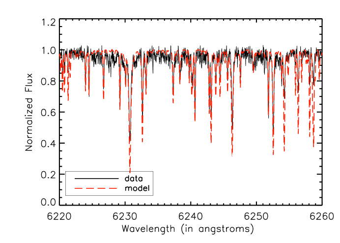
Figure 4: Observed normalized spectra for J2343$+$29 (solid black line) plotted across the wavelength region of 6220–6260 Å. Overplotted is the modelled spectra (red dash line) obtained from PARAS SPEC analysis, with temperature value of $T\rm{{}_{eff}}$ of 5125 K, $[Fe/H]$ of $+0.1$ and ${\rm log}~{}g$ of 4.6.

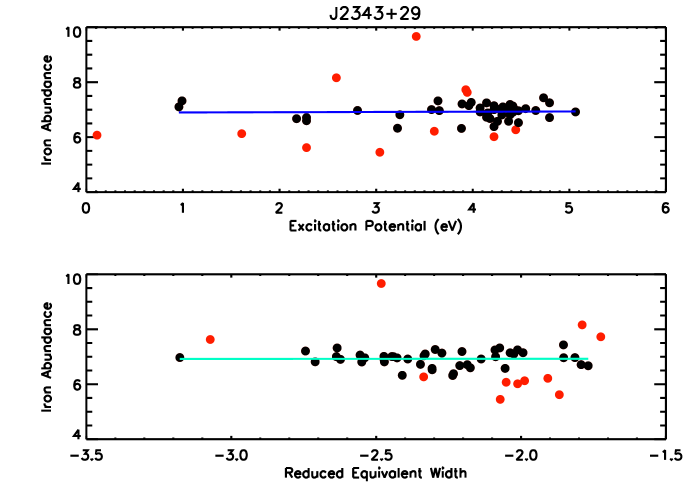
Figure 5: (Top panel) Iron abundance for J2343$+$29 is plotted against excitation potential for each Fe I or Fe II line from the line list. The blue line is the fit to each data point seen in the scatter plot indicating the least slope for the best determined model temperature. (Bottom panel) Iron abundance is plotted against reduced EW and the blue-green line indicates the least slope for best determined model microturbulent velocity. The red points are the discarded points having standard deviation beyond 1 $\sigma$ (not considered for the fit). The best-fit determined parameters are: $T\rm{{}_{eff}}$=5125 K, $[Fe/H]$=0.1, ${\rm log}~{}g$ = $4.6$, $v_{\rm{micro}}$=1.2 km s^-1

We co-added 28 PARAS observed spectra for the source to get a S/N of 65-70 in the blue end (5000–6000 $\AA$). The S/N, as mentioned in §4.3.1, is insufficient for the synthetic spectral fitting method to operate in the blue end. Hence, we concentrated on the red end of the CCD (6000–6500 $\AA$) where the S/N for the co-added spectra is $\sim$ 85 pixel^-1. We determined $T_{\rm{eff}}$ and $[Fe/H]$ by the synthetic spectral fitting method but ${\rm log}~{}g$ could not be determined by this method due to omission of the wavelength region having Mg lines (5160–5190 $\AA$). The stellar parameters obtained from spectral fitting are $T_{\rm{eff}}=5100\pm 84$ K and $[Fe/H]=0.1\pm~{}0.14$. We then applied the EW method on the star J2343$+$29 and calculated $T_{\rm{eff}}$, ${\rm log}~{}g$ and v_micro. The spectral properties determined by PARAS SPEC EW method for J2343$+$29 are: $T_{\rm{eff}}=5125\pm 67$ K, $[Fe/H]=0.1\pm~{}0.14$, ${\rm log}~{}g=4.6\pm 0.14$ and v${}_{\rm{micro}}=1.2~{}\pm$0.1 km s^-1. The $T_{\rm{eff}}$ determined for the star is close to the photometrically derived $T_{\rm{eff}}$ as given in Collier Cameron et al. (2007). The best-fit model spectra determined for J2343$+$29 is shown in Fig. 4. The black solid line indicates the observed normalized spectra from PARAS, and overlaid red dashed line is the best-fit model determined from this work. In Fig. 5, a least squares slope ($0.01_{-0.01}^{+0.02}$) for iron abundances vs. excitation potential indicative of best-fit $T_{\rm{eff}}$ for J2343$+$29 is shown in the upper panel. In the bottom panel, a plot of iron abundance vs reduced EW is shown for the least square slope ($0.005_{-0.005}^{+0.009}$) for best-fit v_turb.

4.4.2 SOPHIE spectra

We used a single SOPHIE reduced spectra having a S/N above 80 in the wavelength region 6000–6500 Å. The synthetic spectral fitting was utilized to determine the $T_{\rm{eff}}$=$5000\pm 84$ K and $[Fe/H]=0.2\pm~{}0.14$. We also worked with the EW method on the star J2343$+$29 and the spectral properties obtained are: $T_{\rm{eff}}$ = 5150$~{}\pm~{}67$ K, $[Fe/H]$ = $0.2~{}\pm~{}0.14$, ${\rm log}~{}g$ = $4.5~{}\pm~{}0.14$ and v_micro=1.2 $\pm$0.1 km s^-1. Thus the results derived for the stellar parameters by both the methods (EW and spectral fitting) from both PARAS and SOPHIE spectra are consistent within error bars as shown in Table 6. It is to be noted that the results obtained from EW method on the PARAS spectra have been used for further analysis.

5 Discussion

Based on spectral analysis and models from EXOFAST, we have determined the mass and radius, and thereby the spectral type of the primary star to be K1. With an angle of inclination determined to be $89.55_{-0.40}^{+0.12}$, and an RV semi-amplitude (K) of $8407_{-10}^{+11}$ from the combined fit to spectroscopic and photometric data, we derive the mass of the secondary star to be $0.098~{}\pm~{}0.007~{}M_{\sun}$.

We use the primary star’s $T_{\rm{eff}}$ and spectral type to estimate the absolute magnitude of the star as $\sim 6.4$ mag (Cox, 2000). Hence, the distance to the star is $\sim$80 pc, indicative of it being in the solar neighborhood. Meibom et al. (2015) have predicted the age of Sun like stars in solar neighbourhood based on their rotational periods. In order to get a handle on the age of the system, we must determine the rotational period of the star. Based on the width of the CCF and the formulation given in Queloz et al. (1998), we determine a $v\sin i$ of $3.2~{}\pm 0.5$ km s^-1 Since the radius of the primary star is $\sim 0.85~{}R_{\sun}$, we calculate a rotational period of $13.6\pm 0.5$ d. The calculated rotational period of the star helps us estimate the age of the star to be between $1.5\pm 0.5$ Gyr (Meibom et al., 2015).

From Baraffe et al. (2015) models, the theoretical radius for a $\sim$$0.098~{}M_{\sun}$ star turns out to be $0.12\pm 0.01~{}R_{\sun}$. The radius of the secondary companion, determined from observations based on transit depth, is $0.127\pm 0.007~{}R_{\sun}$. Although the observational value of radius is dependent on the accuracy of the models used, within the error bars of the orbital fitting, we can conclude that we see almost no discrepancy associated between the observed and theoretically derived radius values. To be precise, the parameters should not be used as test of models, however they are in fact consistent with what the models predict. This substantiates the claim by López-Morales (2007) that observations for stars sufficiently less than $0.3~{}M_{\sun}$ match well within the models. However, in order to examine the M-R relation in the VLMS region, it is very important to increase the statistical sample size of such objects with high-precision measurements. The q ($=M_{2}/M_{1}$) of this system is $\sim 0.1$, which is a rarity among short orbital period EBs (see Figure 9 of Wisniewski et al. (2012)). Due to the low mass ratio, this object seems to reside in a mass ratio-period deficit for low mass stellar binaries. Short period, low q companions are more probable to be found around F type stars, rather than G or K primaries. Over the last few years, a handful of F+M binaries have been discovered and their properties determined (e.g. Pont et al. 2005a; Pont et al. 2005b; 2006 2006; Chaturvedi et al. 2014). Bouchy et al. (2011a, b) suggest that for a massive companion to exist around a primary star, the total angular momentum must be above a critical value. If a primary star has a smaller spin period than the orbital period of the system (as in the case for G-type stars), the tidal interactions between the two stars will cause the secondary companion to be eventually engulfed by the primary. However, this is less likely to occur among fast rotating F-type stars, which have weaker magnetic braking, and can avoid the spin-down caused by tidal effect of the massive secondary. As shown by Zahn (1977) and references therein, the orbital separation of the system will decay only if the spin period of the star is larger than the orbital period of the system. Since, the rotational period of J2343$+$29 is 13.3 d, which is smaller than the orbital period of 16.953 d, we envisage a stable orbit for the system. Out of the 26 sources indicated in Table 1, only three of them (marked in bold) are G/K+M systems. EB J2343$+$29 is the fourth such system studied. We emphasize that a variety of similar EBS with a VLMS component should be studied in detail to assess our understanding of evolutionary mechanism of such systems. The orbital fitting errors reported here are dependent on the models in the SB₁ system. In general, M dwarfs are pronounced to have the discrepancy in observationally measured and theoretically derived radius values. However, this problem is not restricted to VLMS; solar-mass stars also fail to reproduce observations to a great extent (Feiden G.A., 2015) and references therein. Thus, this star serves as a benchmark VLMS, and a prime candidate for future followup as an SB₂, to better constrain the mass and radii of the components and thereby models of stellar structure and evolution.

6 Conclusions

The important conclusions of this work are as follows:

1. Stellar parameters determined for the primary using spectroscopic analysis suggest that the star has $T_{\rm{eff}}$ = 5125$~{}\pm~{}67$ K, $[Fe/H]$ = $0.1~{}\pm~{}0.14$ and ${\rm log}~{}g$ = $4.6~{}\pm~{}0.14$. Hence, the primary has a mass of $0.864_{-0.098}^{+0.097}$ M$\odot$ and a radius of $0.854_{-0.060}^{+0.050}$ R$\odot$.

2. High resolution spectroscopy taken with PARAS, combined with SOPHIE archival RV data and SW archival photometric data, yield an RV semi-amplitude for the source as $8407_{-10}^{+11}$. The secondary mass from RV measurements is $M_{B}~{}=~{}0.098~{}\pm 0.007~{}M_{\sun}$ with an accuracy of $\sim~{}7$ per cent (model dependent). Hence, we conclude that J2343$+$29 is an EB with a K1 primary and a M7 secondary (Pecaut & Mamajek, 2013). The period of the EB, based on combined RV and SW photometry measurements, is revised to be 16.953 d, compared to the previously reported value of 4.24 d.

3. We fit the light curve data simultaneously with RV data and determine the transit depth to be $25$ mmag. Based on the transit depth, the radius of the secondary is estimated as $R_{B}~{}=0.127\pm 0.007~{}R_{\sun}$ with an accuracy of $\sim~{}7$ per cent (model dependent). The observed radius is consistent with the theoretically derived radius values from Baraffe models.

Table 1: A compilation of known VLMS other than our work for masses and radii measured at accuracies better than or at best equal to 10$\%$.

Object	Mass	Radius	EB System	References
J1219-39B	$0.091\pm 0.002$	$0.1174_{-0.0050}^{+0.0071}$	K+M	(1)
HAT-TR-205	$0.124\pm 0.01$	$0.167\pm 0.006$	F+M	(2)
KIC 1571511B	$0.14136^{+0.0051}_{-0.0042}$	$0.17831_{-0.0016}^{+0.0013}$	F+M	(3)
WTS19g4-020B	$0.143\pm 0.006$	$0.174\pm 0.006$	M+M	(4)
J0113+31B	$0.186\pm 0.010$	$0.209\pm 0.011$	G+M	(5)
T-Lyr1-01622B	$0.198\pm 0.012$	$0.238\pm 0.007$	M+M	(6)
KEPLER16B	$0.20255_{-0.00065}^{+0.00066}$	$0.22623_{-0.00053}^{0.00059}$	K+M	(7)
KOI-126C	$0.2127\pm 0.0026$	$0.2318\pm 0.0013$	M+M	(8)
CM Dra A	$0.2130\pm 0.0009$	$0.2534\pm 0.0019$	M+M	(9)
CM Dra B	$0.2141\pm 0.0010$	$0.2396\pm 0.0015$	M+M	(9)
T-Lyr0-08070B	$0.240\pm 0.019$	$0.265\pm 0.010$	M+M	(6)
KOI-126B	$0.2413\pm 0.003$	$0.2543\pm 0.0014$	M+M	(8)
OGLE-TR-78B	$0.243\pm 0.015$	$0.240\pm 0.013$	F+M	(10)
1RXSJ154727A	$0.2576\pm 0.0085$	$0.2895\pm 0.0068$	M+M	(11)
1RXSJ154727B	$0.2585\pm 0.0080$	$0.2895\pm 0.0068$	M+M	(11)
LSPMJ1112B	$0.2745\pm 0.0012$	$0.2978\pm 0.005$	M+M	(12)
GJ3236B	$0.281\pm 0.015$	$0.3\pm 0.015$	M+M	(13)
LP133-373A	$0.34\pm 0.02$	$0.330\pm 0.014$	M+M	(14)
LP133-373B	$0.34\pm 0.02$	$0.330\pm 0.014$	M+M	(14)
19e-3-08413B	$0.351\pm 0.019$	$0.375\pm 0.020$	M+M	(15)
OGLE-TR-6B	$0.359\pm 0.025$	$0.393\pm 0.018$	F+M	(16)
GJ3236A	$0.376\pm 0.016$	$0.3795\pm 0.0084$	M+M	(13)
19c-3-01405B	$0.376\pm 0.024$	$0.393\pm 0.019$	M+M	(15)
MG1-2056316B	$0.382\pm 0.001$	$0.374\pm 0.002$	M+M	(17)
LSPMJ1112A	$0.3946\pm 0.0023$	$0.3860\pm 0.005$	M+M	(12)
CuCnCB	$0.3980\pm 0.0014$	$0.3908\pm 0.0094$	M+M	(18)

References: (1) Triaud et al. (2013); (2) Beatty et al. (2007); (3) Ofir et al. (2012); (4) Nefs et al. (2013);
(5) Gómez Maqueo Chew et al. (2014); (6)Fernández et al. (2009); (7) Doyle et al. (2011);
(8) Carter et al. (2011); (9) Morales et al. (2009); (10) Pont et al. (2005a); (11) Hartman et al. (2011);
(12) Irwin et al. (2011); (13) Irwin et al. (2009); (14) Vaccaro et al. (2007); (15) Birkby et al. (2012);
(16) Bouchy et al. (2005); (17) Kraus et al. (2011); (18) Ribas et al. (2003)

Table 2: Data on J2343$+$29 by SW photometry as discussed in Collier Cameron (2007)

Parameters	Value
V magnitude	10.7
$T_{\rm{eff}}$	5034 K
Spectral Type	K3
Period (P)	$4.24098$ d
Transit Depth	0.021 mag
Transit Duration ($t/P$)	0.030
Transit Epoch	2453245.1886 HJD
$R_{A}$	$0.85R_{\sun}$
$R_{B}$	$1.2R_{J}$

Table 3: Observation log for the star J2343$+$29 with Mt Abu-PARAS. (See text for details)

UT Date	T-2,400,000	Exp. Time	RV	$\sigma$RV
	(BJD-TDB)	(sec.)	(m s-1)	(m s-1)
2013 Nov 12	56609.15187	1800	$-$15367	35
2013 Nov 13	56610.14686	1800	$-$19126	39
2013 Nov 16	56613.12378	1800	$-$28527	43
2013 Nov 19	56616.16537	1800	$-$27088	29
2013 Dec 16	56643.08719	1800	$-$15443	15
2013 Dec 16	56643.10986	1800	$-$15517	22
2013 Dec 17	56644.07896	1800	$-$19293	45
2013 Dec 19	56646.08593	1800	$-$26868	17
2013 Dec 19	56646.10865	1800	$-$26928	24
2013 Dec 20	56647.09027	1800	$-$28554	29
2013 Dec 22	56649.08018	1800	$-$28379	26
2013 Dec 23	56650.07829	1800	$-$27054	26
2013 Dec 23	56650.10118	1800	$-$27016	40
2014 Jan 11	56669.09172	1800	$-$23005	32
2014 Jan 11	56669.11451	1800	$-$22908	43
2014 Jan 12	56670.08510	1800	$-$20812	37
2014 Jan 12	56670.10783	1800	$-$20825	58
2014 Jan 13	56671.08817	1800	$-$18543	42
2014 Jan 16	56674.09761	1800	$-$12707	53
2014 Jan 17	56675.08732	1800	$-$12219	56

Table 4: Archival data obtained for the star J2343$+$29 from SOPHIE observations.

UT Date	T-2,400,000	Exp. Time	RV	$\sigma$RV
	(BJD-TDB)	(sec.)	(m s-1)	(m s-1)
2006 Aug 31	53978.50771	900	-12981	16
2006 Sep 01	53979.59139	900	-12502	10
2006 sep 02	53980.51167	900	-13410	08
2006 Sep 03	53981.52070	900	-16122	10
2007 Aug 30	54342.57369	1500	-29170	08
2007 Aug 31	54343.51469	1800	-28481	06

Table 5: Results obtained from EXOFAST for J2343$+$29.

Parameter	Units	RV fit only	combined RV-Transit fit
Component A:
$M_{A}$	Mass (M$\odot$)	$0.868_{-0.05}^{+0.07}$	$0.864_{-0.098}^{+0.097}$
$R_{A}$	Radius (R$\odot$)	$0.78_{-0.1}^{+0.11}$	$0.854_{-0.060}^{+0.050}$
$\log(g_{A})$	Surface gravity (cgs)	$4.60_{-0.10}^{+0.098}$	$4.559\pm 0.054$
$T_{\rm{eff}}$	Effective temperature (K)	$5141_{-100}^{+70}$	$5150_{-60}^{+90}$
$[$Fe$/$H$]$	Iron Abundance	$0.089_{-0.098}^{+0.093}$	$0.07_{-0.17}^{+0.008}$
Component B:
$e$	Eccentricity	$0.1599\pm 0.0011$	$0.16100_{-0.0027}^{+0.0015}$
$\omega_{*}$	Argument of periastron (degrees)	$78.05_{-0.58}^{+0.59}$	$77.48_{-1.1}^{+0.85}$
$P$	Period (days)	$16.95347\pm 0.00005$	$16.95350\pm 0.00005$
$a$	Semi-major axis (AU)	$0.124\pm 0.002$ $0.1271_{-0.0049}^{+0.0066}$
$M_{B}$	Mass (M$\odot$)	$0.098_{-0.003}^{+0.005}$	$0.098~{}\pm 0.007$
$R_{B}$	Radius (R$\odot$)	-	$0.127\pm 0.007$
$f(m)$	Mass function ⋆ (M$\sun$)	$0.0789\pm 0.009$
RV Parameters:
$T_{P}$	Time of periastron (BJD)	$2455033.471\pm 0.003$	$2453592.333_{-0.030}^{+0.023}$
$K$	RV semi-amplitude (m/s)	$8399_{-10}^{+11}$	$8407_{-10}^{+11}$
$M_{B}/M_{A}$	Mass ratio	$0.1124\pm 0.0009$	$0.1134_{-0.0060}^{+0.0056}$
$\gamma$	Systemic velocity (m/s)	$-21017\pm 12$	$-21031.4_{-19.}^{+18.}$
Transit Parameters:
$T_{C}$	Time of transit (BJD)	-	$2453592.7443_{-0.0032}^{+0.0027}$
$R_{B}/R_{A}$	Radius of secondary in stellar radii	-	$0.1471_{-0.004}^{+0.005}$
$i$	Inclination (degrees)	-	$89.55_{-0.40}^{+0.12}$
$a/R_{A}$	Semi-major axis in stellar radii	-	$32.1_{-1.7}^{+1.4}$
$\delta$	Transit depth	-	$0.025\pm 0.001$
$T_{14}$	Total duration (minutes)	-	$235\pm 7$

Table 6: Results obtained from Spectral analysis (SF=Spectral Fitting; EW=Equivalent Width Method; LV= Literature Value (Errors represented on each parameter are model dependent as discussed in text). S/N is per pixel S/N at 6000 Å.

Star	Vmag	S/N	$T_{\rm{eff}}$			$[Fe/H]$			${\rm log}~{}g$			$vsini$	Reference
			SF	EW	LV	SF	EW (fixed $[Fe/H]$)	LV	SF	EW	LV
Tauceti	3.5	500	$5400\pm 44$	$5400\pm 47$	$5414\pm 10$	$-0.50\pm 0.07$	$-0.5$	$-0.5\pm 0.01$	$4.40\pm 0.09$	$4.5\pm 0.11$	$4.49\pm 0.03$	$3.0\pm 1.0$	(a)
Sigma Draconis	4.7	250	$5450\pm 44$	$5475\pm 47$	$5400\pm 50$	$-0.1\pm 0.07$	$-0.1$	$-0.20\pm 0.06$	$4.50\pm 0.09$	$4.50\pm 0.11$	$4.5\pm 0.05$	$3.0\pm 1.0$	(b)
Procyon	0.37	550	$6550\pm 44$	$6650\pm 47$	$6554\pm 18$	$0.0\pm 0.07$	$0.0$	$-0.04\pm 0.01$	$3.9\pm 0.09$	$3.9\pm 0.11$	$3.99\pm 0.17$	$5.0\pm 1.0$	(a)
HD9407	6.5	220	$5700\pm 44$	$5725\pm 51$	$5661\pm 30$	$0.0\pm 0.11$	$0.0$	$0.03\pm 0.09$	$4.4\pm 0.09$	$4.35\pm 0.11$	$4.42\pm 0.11$	$3.0\pm 1.0$	(c)
HD 166620	6.4	160	$5200\pm 62$	$5025\pm 51$	$4966\pm 205$	$0.0\pm 0.11$	$0.0$	$-0.17\pm 0.08$	$4.6\pm 0.09$	$4.35\pm 0.14$	$4.45\pm 0.17$	$4.0\pm 1.0$	(c)
NLTT 25870	10.01	80	$5400\pm 84$	$5225\pm 67$	$5326\pm 45$	$0.3\pm 0.14$	$0.3$	$0.4\pm 0.07$	-	$4.6\pm 0.14$	$4.45\pm 0.08$	$3.0\pm 1.0$	(d)
HD 285507	10.5	60	$4650\pm 120$	$4450\pm 109$	$4542\pm 50$	$0.1\pm 0.14$	$0.1$	$0.13\pm 0.05$	-	-⋆	$4.67\pm 0.14$	$3.0\pm 1.0$	(e)
KID 5108214	7.94	100	$6000\pm 84$	$6050\pm 67$	$5844\pm 75$	$0.3\pm 0.14$	$0.3$	$0.2\pm 0.1$	$4.0\pm 0.14$	$3.95\pm 0.11$	$3.80\pm 0.01$	$5.0\pm 1.0$	(f)
HD 49674	8.10	90	$5650\pm 84$	$5600\pm 67$	$5632\pm 31$	$0.2\pm 0.11$	$0.2$	$0.33\pm 0.01$	-	$4.35\pm 0.14$	$4.48\pm 0.12$	$3.0\pm 1.0$	(g)
J2343$+$29 (PARAS)	10.7	85	$5100\pm 84$	$5125\pm 67$	$5034$	$0.1\pm 0.14$	$0.1$	–	–	$4.6\pm 0.14$	–	$3.0\pm 1.0$	(h)
J2343$+$29 (SOPHIE)	10.7	90	$5000\pm 84$	$5150\pm 67$	$5034$	$0.2\pm 0.14$	$0.2$	–	–	$4.5\pm 0.14$	–	$3.0\pm 1.0$	(h)

References: (a) Blanco-Cuaresma et al. (2014); (b) Soubiran et al. (2010); (c) Palateou et al. (2015); (d) Butler et al. (2000); (e) McDonald et al. (2012);
(f) KEPLER CFOP (https://cfop.ipac.caltech.edu); (g) Ghezzi et al. (2014); (h) Collier Cameron et al. (2007)
^⋆ No Fe II lines were shortlisted for EW determination.

Figure 1: Mass-Radius diagram for M dwarfs based on Baraffe models (Baraffe et al., 2015) for 1 Gyr isochrone and solar metallicity. Overplotted are the previously studied M dwarfs listed in Table 1 with black filled circles with their reported uncertainties.

Figure 3: (Top panel) Observed transit data obtained from SuperWasp data for the period between October 2004 and December 2006. The transit model obtained from EXOFAST is overplotted on the data points. The fit here shows the case of ”combined RV-Transit photometry” as described in Table 4. (Bottom panel) Observed-Fit residuals are plotted. For better visual representation, the x axis in Phase is shifted by 0.25 so that the central primary transit crossing point (T_c) occurs at phase 0.25 instead of 0. P indicates the period.

References

- Baraffe et al. (2015) Baraffe I., Homeier D., Allard F., Chabrier G. 2015, A&A,577, 42
- Blackwell et al. (1984) Blackwell, D. E., Booth A. J., Petford A. D. 1984, A&A, 132, 236
- Birkby et al. (2012) Birkby J., Nefs B., Hodgkin S., Kovács G., Sipőcz B., Pinfield D., Snellen I., Mislis D., et al. 2012, MNRAS, 426, 1507
- Beatty et al. (2007) Beatty T. G., Fernández J. M., Latham D. W., Bakos G. Á., Kovács G., Noyes R. W. Stefanik R. P., et al. 2007, ApJ, 663, 573
- Blanco-Cuaresma et al. (2014) Blanco-Cuaresma S., Soubiran C., Heiter U., Jofre P. 2014, A&A, 569, 111
- Boisse et al. (2010) Boisse I., Eggenberger A., Santos N. C., Lovis C., Bouchy F., Hébrand G., Arnold L., Bonfils X., et al. 2010, A&A, 523, 88
- Bouchy et al. (2001) Bouchy F., Pepe F., Queloz D. 2001, A&A, 374, 733
- Bouchy et al. (2005) Bouchy F., Pont F., Melo C., Santos N. C., Mayor M., Queloz D., Udry S. 2005, A&A, 431, 1105
- Bouchy et al. (2011a) Bouchy F., Deleuil M., Guillot T., Aigrain S., Carone L., Cochran W. D., Almenara J. M., Alonso R., et al. 2011a, A&A, 525, 68
- Bouchy et al. (b) Bouchy F., Bonomo A. S., Santerne A., Moutou C., Deleuil M., Diaz M., Eggenberger A., Ehrereich D., et al. 2011b, A&A, 533, 83
- Butler et al. (2000) Butler R. P., Vogt S. S., Marcy G. W., Fischer D. 2000, ApJ, 545, 504
- Carter et al. (2011) Carter J. A., Fabrycky D. C., Ragozzine D., Holman M. J., Quinn S. N., Latham D. W., Buchhave L. A., Van Cleve J., et al. 2011, Science, 331, 562
- Chabrier et al. (2007) Chabrier G., Gallardo J., Baraffe I. 2007, A&A, 472, L17
- Chakraborty et al. (2014) Chakraborty A., Mahadevan S., Roy A., Dixit V., Richardson E. H., Dongre V., Pathan F., Chaturvedi P., et al. 2014, PASP, 126, 133
- Chaturvedi et al. (2014) Chaturvedi P., Deshpande R., Dixit V., Roy A., Chakraborty A., Mahadevan S., Anandarao B. G., Hebb L., et al. 2014, MNRAS, 442, 3737
- Christian et al. (2006) Christian D. J., Pollacco D. L., Skillen I., Street R A., Keenan F. P., Clarkson W. I., Collier Cameron A., Kane S. R., et al. 2006, MNRAS, 372, 1117
- Collier Cameron et al. (2007) Collier Cameron A., Wilson D. M., West R. G., Hebb L., Wang X. B., Aigrain S., Bouchy F., Christian D. J., et al. 2007, MNRAS, 380, 1230
- Cox (2000) Cox A. 2000, Allen’s Astrophysical Quantities, AIP Press
- Doyle et al. (2011) Doyle L. R., Carter J. A., Fabrycky D. C., Slawson R. W., Howell S. B., Winn J. N., Orosz J. A., Prćaronsa A. et al. 2011, Science, 333, 1602
- Eastman, Gaudi & Agol (2013) Eastman J., Gaudi B. S., & Agol E. 2013, PASP, 125, 83
- Feiden G.A. (2015) Feiden G. A. 2015, ASPC, 496, 137
- Fernández et al. (2009) Fernández J. M., Latham D. W., Torres G., Everett M. E., Mandushev G., Charbonneau D., O’Donovan F. T., Alonso, R. et al. 2009, ApJ, 701, 764
- Ghezzi et al. (2014) Ghezzi L., Dutra-Ferreira D., Lorenzo-Oliveira D., Porto De Mello G. F., Santiago B. X., De Lee N., Lee B. L., da Costa L. N. 2014, AJ, 148, 105
- Gómez Maqueo Chew et al. (2014) Gómez Maqueo Chew Y., Morales J. C., Faedi F., García-Melendo E., Hebb L., Rodler F., Deshpande R., Mahadevan S. et al. 2014 A&A, 572, 50
- Gray et al. (1999) Gray R. O. 1999, ’SPECTRUM: A stellar spectral synthesis program’, Astrophysics Source Code Library
- Gray (2009) Gray R. O. 2009, Documentation for Spectrum v2.76, Appalachian State University
- Hartman et al. (2011) Hartman J. D., Bakos G. Á., Noyes R. W., Sipőcz B., Kovács G., Mazeh T., Shporer A., Pál A. 2011, AJ, 141, 166
- Irwin et al. (2009) Irwin J., Charbonneau D., Berta Z. K., Quinn S. N., Latham D. W., Torres G., Blake C. H., Burke C. J. et al. 2009, ApJ, 701, 1436
- Irwin et al. (2011) Irwin J. M., Quinn S. N., Berta Z. K., Latham D. W., Torres G., Burke C. J., Charbonneau D., Dittmann, J. et al. 2011, ApJ, 742, 123
- Johnson et al. (2011) Johnson J. A., Payne M., Howard A. W., Clubb K. I., Ford E. B., Bowler B. P., Henry G. W., Fischer D. A., et al. 2011, AJ, 141, 16
- Kallrath et al. (2000) Kallrath J., Milone E. F. Eclipsing binary stars : modelling and analysis, The Observatory, Springer, 120
- Kraus et al. (2011) Kraus A. L., Tucker R. A., Thompson M. I., Craine E. R., Hillenbrand L. A. 2011, AJ, 728, 48
- Kurucz (1993) Kurucz R. L. 1993, CD-ROM 13, ATLAS9 Stellar Atmosphere Programs and 2km/sec Grid (Cambridge: Smithsonian Astrophys. Obs.)
- López-Morales (2007) López-Morales M. 2007, ApJ, 660, 732
- McDonald et al. (2012) McDonald I., Zijlstra A., Boyer M. L. 2012, MNRAS, 427, 343
- Meibom et al. (2015) Meibom S., Barnes S., Platais I., Gilliland R. G., Latham D. W., Mathieu R. D. 2015, Nature, 571, 589
- Morales et al. (2009) Morales J. C., Ribas I., Jordi C., Torres G., Gallardo J., Guinan E. F., Charbonneau D., Wolf M., Latham D. W., et al. 2009, ApJ, 691, 1400
- Nefs et al. (2013) Nefs S. V., Birkby J. L., Snellen I. A. G., Hodgkin S. T., Sipőcz B. M., Kovács G. Milis D., Pinfield D. J. et al. 2013, mnras, 431, 3240
- Ofir et al. (2012) Ofir A., Gandolfi D., Buchhave L., Lacy C. H. S., Hatzes A. P., Fridlund M. 2012, MNRAS, 423, L1
- Piskunov & Valenti (2002) Piskunov N. & Valenti J. 2002, A&A, 385, 1095
- Pecaut & Mamajek (2013) Pecaut M. J. & Mamajek E. E. 2013, ApJS, 208, 9
- Palateou et al. (2015) Palateou F., Gebran M., Houdebine E. R., Watson V. 2015, A&A, 580, 78
- Pepe et al. (2002) Pepe F., Mayor M., Galland F., Naef D., Queloz D., Santos N. C., Udry S., Burnet M. 2002, A&A, 388, 632
- Pont et al. (2005a) Pont F., Bouchy F., Melo C., Santos N. C., Mayor M., Queloz D., Udry S. 2005a, A&A, 438, 1123
- Pont et al. (2005b) Pont F., Melo C.H.F., Udry S., Queloz D., Mayor M., Santos N.C. 2005b, A&A, 433, L21
- (46) Pont F., Moutou C., Bouchy F., Behrend R., Mayor M., Udry S., Queloz D., Santos N. C., et al. 2006, A&A, 447, 1035
- Queloz et al. (1998) Queloz D., Allain S., Mermilliod J.-C., Bouvier J., Mayor M. 1998, AA, 335, 183
- Ribas et al. (2003) Ribas I. 2003, A&A, 398, 239
- Soubiran et al. (2010) Soubiran C., Le Campion J.-F., Cayrel de Strobel G., Caillo A. 2010, A&A, 515, 111
- Sousa et al. (2014) Sousa S. G., Santos N. C., Adibekyan V., Delgado-Mena E., Tabernero H. M., Gonzalez Hernandez J. I., Montes D., Smilijanic R. 2014, A&A, 561, 21
- Street et al. (2007) Street R. A., Christian D. J., Clarkson W. I., Collier Cameron A., Enoch B., Kane S. R., Lister T. A., West R. G. 2007, MNRAS, 379, 816
- Tal-Or et al. (2013) Tal-Or L., Mazeh T., Alonso R., Bouchy F., Cabrera J., Deeg H. J., Deleuil M., Faigler S. 2013, A&A, 553, 30
- Torres, Andersen & Giménez (2010) Torres G., Andersen J., Giménez A. 2010, A&ARv, 18, 67
- Triaud et al. (2013) Triaud A. H. M. J., Hebb L., Anderson D. R., Cargile P., Collier Cameron A., Doyle A. P., Faedi F., Gillon M. 2012, A&A, 549, 18
- Vaccaro et al. (2007) Vaccaro T. R., Rudkin M., Kawka A., Vennes S., Oswalt T. D., Silver I., Wood M., Smith J. A. 2007, ApJ, 661, 1112
- Valenti & Piskunov (1996) Valenti J. A. & Piskunov N. 1996, ApJS, 118, 595
- Valenti & Fischer (2005) Valenti J. A. & Fischer D. A. 2005, ApJS, 159, 141
- Wisniewski et al. (2012) Wisniewski J., Ge J., Crepp J. R., Lee N., Eastman J., Esposito M., Fleming S. 2012, AJ, 143, 107
- West et al. (2009) West R. G., Collier Cameron A., Hebb L., Joshi, Y. C., Pollacco D., Simpson E., Skillen I., Stempels H. C., et al. 2009, A&A, 502, 395
- Zahn (1977) Zahn J. P. 1977, A&A, 57, 383