Scheduling massively parallel multigrid for multilevel Monte Carlo Methods

Abstract

The computational complexity of naive, sampling-based uncertainty quantification for 3D partial differential equations is extremely high. Multilevel approaches, such as multilevel Monte Carlo (MLMC), can reduce the complexity significantly, but to exploit them fully in a parallel environment, sophisticated scheduling strategies are needed. Often fast algorithms that are executed in parallel are essential to compute fine level samples in 3D, whereas to compute individual coarse level samples only moderate numbers of processors can be employed efficiently. We make use of multiple instances of a parallel multigrid solver combined with advanced load balancing techniques. In particular, we optimize the concurrent execution across the three layers of the MLMC method: parallelization across levels, across samples, and across the spatial grid. The overall efficiency and performance of these methods will be analyzed. Here the ”scalability window” of the multigrid solver is revealed as being essential, i.e., the property that the solution can be computed with a range of process numbers while maintaining good parallel efficiency. We evaluate the new scheduling strategies in a series of numerical tests, and conclude the paper demonstrating large 3D scaling experiments.

1 Introduction

Data uncertainties are ubiquitous in many application fields, such as subsurface flow or climate prediction. Inherent uncertainties in input data propagate to uncertainties in quantities of interest, such as the time it takes pollutants leaking from a waste repository to reach a drink water well. This situation has driven the development of novel uncertainty quantification (UQ) methods; most commonly, using partial differential equations (PDEs) to model the physical processes and stochastic models to incorporate data uncertainties. Simulation outputs are then statistics (mean, moments, cumulative distribution function) of the quantities of interest. However, typical sampling-and-averaging techniques for computing statistics quickly become infeasible, when each sample involves the numerical solution of a PDE.

1.1 Mathematical model and UQ methods

Let us consider an abstract, possibly nonlinear system of PDEs with uncertain data

$$\mathcal{M}(u;\omega)\ =\ 0,$$ (1)

where the solution $u$ is sought in some suitable space $V$ of functions $v:D\subset\mathbb{R}^{d}\to\mathbb{R}^{k}$ with $k\in\mathbb{N}$ and $D$ open and bounded, subject to suitable boundary conditions. $\mathcal{M}$ is a differential operator depending on a set of random parameters parametrised by an element $\omega$ of the abstract sample space $(\Omega,\mathcal{F},\mathbb{P})$ that encapsulates the uncertainty in the data, with $\Omega$ the set of all outcomes, $\mathcal{F}$ the $\sigma$-algebra (the “set” of all events), and $\mathbb{P}$ the associated probability measure. As a consequence the solution $u$ itself is a random field, i.e. $u=u(x,\omega)$, with realizations in $V$.

We are typically only interested in functionals $Q(u)\in\mathbb{R}$ of $u$. To compute them we need to approximate the solution $u$ numerically, e.g. using finite element methods, which introduces bias error. The cost $\mathcal{C}$ typically grows inverse proportionally to some power of the bias error, i.e. $\mathcal{C}=\mathcal{O}(\varepsilon^{-r})$ where $\varepsilon$ denotes the bias error tolerance. This is a challenging computational task that requires novel methodology combined with cutting-edge parallel computing for two reasons: firstly, real life applications lead to PDE systems in three dimensions that often can only be solved effectively and accurately on a parallel computer (even without data uncertainties); secondly, typical uncertainties in applications, such as a random diffusion coefficient $k(x,\omega)$, are spatially varying on many scales and cannot be described by a handful of stochastic parameters. This limits considerably the types of UQ methods that are applicable.

For low dimensional problems, stochastic Galerkin, stochastic collocation and polynomial chaos methods have been shown to provide efficient and powerful UQ tools (see, e.g., [13, 42, 26] and the references therein), but in general their complexity grows exponentially with the stochastic dimension. The cost of sampling methods, such as, e.g., Monte Carlo, does not grow with the stochastic dimension, but classical Monte Carlo is notoriously slow to converge. Multilevel Monte Carlo (MLMC) simulation [14, 6] can help to significantly accelerate the convergence. It has been applied and extended to a range of applications, see [2, 28, 7, 11, 22].

The idea of MLMC is to reduce algorithmic complexity by performing as much computational work as possible on coarse meshes. To this end, MLMC uses a hierarchy of discretisations of (1) of increasing accuracy to estimate statistics of $Q(u)$ more efficiently, i.e. using a large number of coarse samples to fully capture the variability, but only a handful of fine samples to eliminate the bias due to the spatial discretisation. Here, we employ multilevel methods not only to accelerate the stochastic part, but also to provide a scalable solver for individual realizations of (1).

1.2 Parallel methods and algorithms

Current leading-edge supercomputers provide a peak performance in the order of a hundred petaflop/s (i.e. $10^{17}$ floating point operations per second) [33]. However, all these computers draw their computational power from parallelism, with current processor numbers already at $P_{\text{max}}\approx 10^{7}$ see [9]. The technological trend indicates that future exascale computers may use $P_{\text{max}}\approx 10^{9}$. Consequently, designing efficient fast parallel algorithms for high performance computers is a challenging task today and will be even more so in the future.

MLMC methods are characterized by three algorithmic levels that are potential candidates for parallel execution. As in a standard Monte Carlo method, the algorithm uses a sequence of classical deterministic problems (samples) that can be computed in parallel. The size of these subproblems varies depending on which level of resolution the samples are computed on. We therefore distinguish between parallelism within an MLMC level and parallelism across MLMC levels. The third algorithmic level is the solver for each deterministic PDE problem which can be parallelized itself. Indeed, the total number of samples on finer MLMC levels is typically moderate, so that the first two levels of parallelism will not suffice to exploit $P_{\text{max}}$ processors. Parallel solvers for elliptic PDEs are now able to solve systems with $1.1\text{\times}{10}^{13}$ degrees of freedom on petascale machines [16] with compute times of a few minutes using highly parallel multigrid methods [5, 17]. In this paper, we will illustrate for a simple model problem in three spatial dimensions, how these different levels of parallelism can be combined and how efficient parallel MLMC strategies can be designed.

To achieve this, we extend the massively parallel Hierarchical Hybrid Grids (HHG) framework [3, 19] that exhibits excellent strong and weak scaling behavior [21, 1] to the MLMC setting. We use the fast multigrid solver in HHG to generate spatially correlated samples of the random diffusion coefficient, as well as to solve the resulting subsurface flow problems efficiently. Furthermore, the hierarchy of discretisations in HHG provides the ideal multilevel framework for the MLMC algorithm.

Parallel solvers may not yield linear speedup and the efficiency may deteriorate on a large parallel computer system when the problems become too small. In this case, too little work can be executed concurrently and the scalar overhead dominates. This effect is well-known and can be understood prototypically in the form of Amdahl’s law [21]. In the MLMC context, problems of drastically different size must be solved. In general, a solver, when applied to a problem of given size, will be characterized by its scalability window, i.e., the processor range for which the parallel efficiency remains above an acceptable threshold. Because of memory constraints, the scalability window will open at a certain minimal processor number. For larger processor numbers the parallel efficiency will deteriorate until the scalability window closes. In practice, additional restrictions imposed by the system and the software permit only specific processor numbers within the scalability window to be used.

MLMC typically leads to a large number of small problems, a small number of very large problems, and a fair number of intermediate size problems. On the coarser levels, the problem size is in general too small to use the full machine. The problem is outside the scalability window and solver-parallelism alone is insufficient. On the other hand, the efficiency of parallelization across samples and across levels typically does not deteriorate, since only little data must be extracted from each sample to compute the final result of the UQ problem. However, on finer levels we may not have enough samples to fill the entire machine. Especially for adaptive MLMC, where the number of samples on each level is not known a priori but must be computed adaptively using data from all levels, this creates a challenging load balancing problem.

A large scalability window of the solver is essential to devise highly efficient execution strategies, but finding the optimal schedule is restricted by a complex combination of mathematical and technical constraints. Thus the scheduling problem becomes in itself a high-dimensional, multi-constrained, discrete optimisation problem. Developing suitable approaches in this setting is one of the main objectives of this paper. See [34, 35] for earlier static and dynamic load balancing approaches.

The paper is structured as follows: In Section 2, we briefly review the MLMC method and its adaptive version. Section 3 introduces the model problem. Here, we use an alternative PDE-based sampling technique for Matérn covariances [25, 29] that allows us to reuse the parallel multigrid solver. In Sections 4 and 5, we define a classification of different parallel execution strategies and develop them into different parallel scheduling approaches. In Section 6, we study the parallel efficiency of the proposed strategies and demonstrate their flexibility and robustness, before finishing in Section 7 with large-scale experiments on advanced supercomputer systems.

2 The Multilevel Monte Carlo method

To describe the MLMC method, we assume that we have a hierarchy of finite element (FE) discretisations of (1). Let $\{V_{\ell}\}_{\ell\geq 0}$ be a nested sequence of FE spaces with $V_{\ell}\subset V$, mesh size $h_{\ell}>0$ and $M_{\ell}$ degrees of freedom. In the Hierarchical Hybrid Grids (HHG) framework [3, 19], the underlying sequence of FE meshes is obtained via uniform mesh refinement from a coarsest grid $\mathcal{T}_{0}$, and thus $h_{\ell}\simeq 2^{-\ell}h_{0}$ and $M_{\ell}\simeq 2^{3\ell}M_{0}$ in three space dimensions.

Denoting by $u_{\ell}=u_{\ell}(x,\omega)\in V_{\ell}$ the FE approximation of $u$ on Level $\ell$, we have

$$\mathcal{M}_{\ell}(u_{\ell};\omega)=0,\qquad\ell\geq 0.$$ (2)

Here, the (non)linear operator $\mathcal{M}_{\ell}$ and the functional of interest $Q_{\ell}(u_{\ell},\omega)$ may also involve numerical approximations.

2.1 Standard Monte-Carlo Simulation

The standard Monte Carlo (MC) estimator for the expected value $\mathbb{E}[Q]$ of $Q(u)$ on level $L\geq 0$ is given by

$$\widehat{Q}^{\text{MC},N}_{L}=\frac{1}{N}\sum_{i=1}^{N}Q_{L}^{i}\,,$$ (3)

where $Q_{L}^{i}=Q_{L}(u_{L}^{i},\omega^{i})$, $i=1,\ldots,N$, are $N$ independent samples of $Q_{L}(u_{L})$.

There are two sources of error: (i) The bias error due to the FE approximation. Assuming that $|Q_{L}^{i}-Q(u^{i},\omega^{i})|=\mathcal{O}(M_{L}^{-\alpha})$, for almost all $\omega^{i}$ and a constant $\alpha>0$, it follows directly that there exists a constant $C_{b}$, independent of $M_{L}$, such that

$$|\mathbb{E}[Q_{L}-Q]|\leq C_{b}M_{L}^{-\alpha}\leq\varepsilon_{b}$$ (4)

for $M_{L}\geq(\varepsilon_{b}/C_{b})^{1/\alpha}$ (cf. [36]).

(ii) There is a sampling error due to the finite number $N$ of samples in (3).

The total error is typically quantified via the mean square error (MSE), given by

$$e\left(\widehat{Q}^{\text{MC},N}_{L}\right)^{2}:=\mathbb{E}[(\widehat{Q}^{\text{MC},N}_{L}-\mathbb{E}[Q])^{2}]=\left(\mathbb{E}[Q_{L}-Q]\right)^{2}+N^{-1}\mathbb{V}[Q_{L}],$$ (5)

where $\mathbb{V}[Q_{L}]$ denotes the variance of the random variable $Q_{L}(u_{L})$. The first term in (5) can be bounded in terms of (4), and the second term in is smaller than a sample tolerance $\varepsilon_{s}^{2}$ if $N\geq\mathbb{V}[Q_{L}]\varepsilon_{s}^{-2}$. We note that for $L$ sufficiently large, $\mathbb{V}[Q_{L}]\approx\mathbb{V}[Q]$. To ensure that the total MSE is less than $\varepsilon^{2}$ we choose

$$\varepsilon_{s}^{2}=\theta\varepsilon^{2}\quad\text{and}\quad\varepsilon_{b}^{2}=(1-\theta)\varepsilon^{2},\quad\text{for any fixed}\ \ 0<\theta<1.$$ (6)

Thus, to reduce (5) we need to choose a sufficiently fine FE mesh and a sufficiently large number of samples. This very quickly leads to an intractable problem for complex PDE problems in 3D. The cost for one sample $Q_{L}^{i}$ of $Q_{L}$ depends on the complexity of the FE solver and of the random field generator. Typically it will grow like $C_{c}M_{L}^{\gamma}$, for some $\gamma\geq 1$ and some constant $C_{c}$, independent of $i$ and of $M_{L}$. Thus, the total cost to achieve a MSE $e(\widehat{Q}_{L}^{\text{MC},N})^{2}\leq\varepsilon^{2}$ (the $\varepsilon$-cost) is

$$\text{Cost}\left(\widehat{Q}_{L}^{\text{MC},N}\right)=\mathcal{O}(M^{\gamma}N)=\mathcal{O}(\varepsilon^{-2-\gamma/\alpha}).$$ (7)

For the coefficient field and for the output functional studied below, we have only $\alpha=1/6$. In that case, even if $\gamma=1$, to reduce the error by a factor 2 the cost grows by a factor of $2^{8}=256$, which quickly leads to an intractable problem even in a massively parallel environment.

2.2 Multilevel Monte-Carlo Simulation

Multilevel Monte Carlo (MLMC) simulation [14, 6, 2] seeks to reduce the variance of the estimator and thus to reduce computational time, by recursively using coarser FE models as control variates. By exploiting the linearity of the expectation operator, we avoid estimating $\mathbb{E}[Q]$ directly on the finest level $L$ and do not compute all samples to the desired accuracy (bias error). Instead, using the simple identity $\mathbb{E}[Q_{L}]=\mathbb{E}[Q_{0}]+\sum_{\ell=1}^{L}\mathbb{E}[Y_{\ell}]$, we estimate the mean on the coarsest level (Level $0$) and correct this mean successively by adding estimates of the expected values of $Y_{\ell}(\omega):=Q_{\ell}(u_{\ell},\omega)-Q_{\ell-1}(u_{\ell-1},\omega)$, for $\ell\geq 1$. Setting $Y_{0}:=Q_{0}$, the MLMC estimator is then defined as

$$\widehat{Q}_{L}^{\text{ML}}:=\sum_{\ell=0}^{L}\widehat{Y}^{\text{MC},N_{\ell}}_{\ell}\,,$$ (8)

where the numbers of samples $N_{\ell}$, $\ell=0,\ldots,L$, are chosen to minimize the total cost of this estimator for a given prescribed sampling error (see Eqn. (11) below). Note that we require the FE solutions $u_{\ell}(x,\omega^{i})$ and $u_{\ell-1}(x,\omega^{i})$ on two levels to compute a sample $Y^{i}_{\ell}$ of $Y_{\ell}$, for $\ell\geq 1$, and thus two PDE solves, but crucially both with the same $\omega^{i}$ and thus with the same PDE coefficient (see Algorithm 1).

Algorithm 1 Multilevel Monte Carlo.

1.	For all levels $\ell=0,\ldots,L$ do
	a.	For $i=1,\ldots,N_{\ell}$ do
		i.  Set up (2) for $\omega^{i}$ on Level $\ell$ and $\ell-1$ (if $\ell>0$).
		ii. Compute $u_{\ell}(\omega^{i})$ and $u_{\ell-1}(\omega^{i})$ (if $\ell>0$), as well as $Y^{i}_{\ell}$.
	b.	Compute $\widehat{Y}^{\mathrm{MC},N_{\ell}}_{\ell}=\frac{1}{N_{\ell}}\sum_{i=1}^{N_{\ell}}Y^{i}_{\ell}$.
2.	Compute $\widehat{Q}_{L}^{\text{ML}}$ using (8).

The cost of this estimator is

$$\text{Cost}(\widehat{Q}_{L}^{\text{ML}})=\sum_{\ell=0}^{L}N_{\ell}\mathcal{C}_{\ell}\,,$$ (9)

where $\mathcal{C}_{\ell}$ is the cost to compute one sample of $Y_{\ell}$ on level $\ell$. For simplicity, we use independent samples across all levels, so that the $L+1$ standard MC estimators in (8) are independent. Then, the MSE of $\widehat{Q}_{L}^{\text{ML}}$ simply expands to

$$e\left(\widehat{Q}_{L}^{\text{ML}}\right)^{2}=\big{(}\mathbb{E}[Q_{L}-Q]\big{)}^{2}\;+\;\sum_{l=0}^{L}N_{\ell}^{-1}\mathbb{V}[Y_{\ell}]\,.$$ (10)

This leads to a hugely reduced variance of the estimator since both FE approximations $Q_{\ell}$ and $Q_{\ell-1}$ converge to $Q$ and thus $\mathbb{V}[Y_{\ell}]\to 0$, as $M_{\ell-1}\to\infty$.

By choosing $M_{L}\geq(\varepsilon_{b}/C_{b})^{-1/\alpha}$, we can ensure again that the bias error is less than $\varepsilon_{b}$, but we still have some freedom to choose the numbers of samples $N_{\ell}$ on each of the levels, and thus to ensure that the sampling error is less than $\varepsilon_{s}^{2}$. We will use this freedom to minimize the cost $\text{Cost}(\widehat{Q}_{L}^{\text{ML}})$ in (9) subject to the constraint $\sum_{\ell=0}^{L}N_{\ell}^{-1}\mathbb{V}[Y_{\ell}]=\varepsilon_{s}^{2}$, a simple discrete, constrained optimization problem with respect to $N_{0},\ldots,N_{L}$ (cf. [14, 6]). It leads to

$$N_{\ell}\ =\ \varepsilon_{s}^{-2}\left(\sum_{\ell=0}^{L}\sqrt{\mathbb{V}[Y_{\ell}]\mathcal{C}_{\ell}}\right)\,\sqrt{\frac{\mathbb{V}[Y_{\ell}]}{C_{\ell}}}.$$ (11)

Finally, under the assumptions that

$$\mathcal{C}_{\ell}\;\leq\;C_{c}M_{\ell}^{\gamma}\quad\text{and}\quad\mathbb{V}[Y_{\ell}]\leq C_{v}\,M_{\ell}^{-\beta}\,,$$ (12)

for some $0<\beta\leq 2\alpha$ and $\gamma\geq 1$ and for two constants $C_{c}$ and $C_{v}$, independent of $i$ and of $M_{\ell}$, the $\varepsilon$-cost to achieve $e(\widehat{Q}_{L}^{\text{ML}})^{2}\leq\varepsilon^{2}$ can be bounded by

$$\text{Cost}(\widehat{Q}_{L}^{\text{ML}})\;=\;\varepsilon_{s}^{-2}\left(\sum_{\ell=0}^{L}\sqrt{\mathbb{V}[Y_{\ell}]\mathcal{C}_{\ell}}\right)^{2}\;\leq\;C_{\text{ML}}\,\varepsilon^{-2-\max\left(0,\frac{\gamma-\beta}{\alpha}\right)}\,.$$ (13)

Typically $\beta\approx 2\alpha$ for smooth functionals $Q(\cdot)$. For CDFs we typically have $\beta=\alpha$.

There are three regimes: $\gamma<\beta$, $\gamma=\beta$ and $\gamma>\beta$. In the case of the exponential covariance, typically $\gamma>\beta$ and $\beta=2\alpha$ and thus $\text{Cost}(\widehat{Q}_{L}^{\text{ML}})=\mathcal{O}(\varepsilon^{-\gamma/\alpha})$, which is a full two orders of magnitude faster than the standard MC method. Moreover, MLMC is optimal for this problem, in the sense that its cost is asymptotically of the same order as the cost of computing a single sample to the same tolerance $\varepsilon$.

2.3 Adaptive Multilevel Monte Carlo

In Algorithm 2 we present a simple sequential, adaptive algorithm from [14, 6] that uses the computed samples to estimate bias and sampling error and thus chooses the optimal values for $L$ and $N_{\ell}$. Alternative adaptive algorithms are described in [15, 7, 11]. For the remainder of the paper we will restrict to uniform mesh refinement, i.e. $h_{\ell}=2^{-\ell}h_{0}$ and $M_{\ell}=\mathcal{O}(8^{\ell}M_{0})$ in 3D.

Algorithm 2 Adaptive Multilevel Monte Carlo.

1.	Set $\varepsilon$, $\theta$, $L=1$ and $N_{0}=N_{1}=N_{\text{Init}}$.
2.	For all levels $\ell=0,\ldots,L$ do
	a.	Compute new samples of $Y_{\ell}$ until there are $N_{\ell}$.
	b.	Compute $\widehat{Y}^{\mathrm{MC},N_{\ell}}_{\ell}$ and $s^{2}_{\ell}$, and estimate $\mathcal{C}_{\ell}$.
3.	Update the estimates for $N_{\ell}$ using (15) and
	if $\widehat{Y}^{\mathrm{MC},N_{L}}_{L}>(8^{\alpha}-1)\varepsilon_{b}$, increase $L\to L+1$ and set $N_{L}=N_{\text{Init}}$.
4.	If all $N_{\ell}$ and $L$ are unchanged,
		Go to 5.
	Else Return to 2.
5.	Set $\widehat{Q}_{L}^{\mathrm{ML}}=\sum_{\ell=0}^{L}\widehat{Y}^{\mathrm{MC},N_{\ell}}_{\ell}$.

To estimate the bias error, let us assume that $M_{\ell}$ is sufficiently large, so that we are in the asymptotic regime, i.e. $|\mathbb{E}[Q_{\ell}-Q]|\approx C_{b}\,M_{\ell}^{-\alpha}$ in (4). Then (cf. [11])

$$|\mathbb{E}[Q_{\ell}-Q]|\leq\frac{1}{8^{\alpha}-1}\widehat{Y}^{\text{MC},N_{\ell}}_{\ell}\,.$$ (14)

Also, using the sample estimator $s^{2}_{\ell}:=\frac{1}{N_{\ell}}\sum_{i=1}^{N_{\ell}}\big{(}Y_{\ell}^{i}-\widehat{Y}^{\text{MC},N_{\ell}}_{\ell}\big{)}^{2}$ to estimate $\mathbb{V}[Y_{\ell}]$ and the CPU times from the runs up-to-date to estimate $\mathcal{C}_{\ell}$, we can estimate

$$N_{\ell}\ \approx\ \varepsilon_{s}^{-2}\left(\sum_{\ell=0}^{L}\sqrt{s^{2}_{\ell}\mathcal{C}_{\ell}}\right)\,\sqrt{\frac{s^{2}_{\ell}}{C_{\ell}}}.$$ (15)

3 Model problem and deterministic solver

As an example, we consider an elliptic PDE in weak form: Find $u(\cdot,\omega)\in V:=H^{1}_{0}(D)$ such that

$$\int_{D}\nabla v(x)\cdot\big{(}k(x,\omega)\nabla u(x,\omega)\big{)}\,\text{d}x=\int_{D}f(x)v(x)\,\text{d}x,\quad\text{for all}\ v\in V\ \text{and}\ \omega\in\Omega.$$ (16)

This problem is motivated from subsurface flow. The solution $u$ and the coefficient $k$ are random fields on $D\times\Omega$ related to fluid pressure and rock permeability. For simplicity, we only consider $D=(0,1)^{3}$, homogeneous Dirichlet conditions and a deterministic source term $f$. If $k(\cdot,\omega)$ is continuous (as a function of $x$) and $k_{\min}(\omega):=\min_{x\in\overline{D}}k(x,\omega)>0$ almost surely (a.s.) in $\omega\in\Omega$, then it follows from the Lax-Milgram Lemma that this problem has a unique solution (cf. [4]). As quantities of interest in Section 7, we consider $Q(u):=u(x^{*})$, for some $x^{*}\in D$, or alternatively $Q(u):=\frac{1}{|\Gamma|}\int_{\Gamma}-k\frac{\partial u}{\partial n}\,\text{d}s$, for some two-dimensional manifold $\Gamma\subset\overline{D}$ can be of interest.

3.1 Discretisation

To discretise (16), for each $\omega\in\Omega$, we use standard $\mathbb{P}_{1}$ finite elements on a sequence of uniformly refined simplicial meshes $\{\mathcal{T}_{\ell}\}_{\ell\geq 0}$. Let $V_{\ell}$ be the FE space associated with $\mathcal{T}_{\ell}$, $\mathcal{N}_{\ell}$ the set of interior vertices, $h_{\ell}$ the mesh size and $M_{\ell}=|\mathcal{N}_{\ell}|$ the number of degrees of freedom. Now, problem (16) is discretised by restricting it to functions $u_{\ell},v_{\ell}\in V_{\ell}$. Using the nodal basis $\{\phi_{j}:x_{j}\in\mathcal{N}_{\ell}\}$ of $V_{\ell}$ and expanding $u_{\ell}(\cdot,\omega):=\sum_{j\in\mathcal{N}_{\ell}}U^{(\ell)}_{j}(\omega)\phi_{j}$, this can be written as a linear equation system where the entries of the system matrix are assembled elementwise based on on a four node quadrature formula

$$A^{(\ell)}(\omega)\mathbf{U}^{(\ell)}(\omega)\,=\,\mathbf{F}^{(\ell)},\quad$$ where

$$A^{(\ell)}_{i,j}(\omega):=\sum_{\tau\in\mathcal{T}_{\ell}}\nabla\phi_{i}\cdot\nabla\phi_{j}\big{|}_{\tau}\,\frac{|\tau|}{4}\,\bigg{(}\sum_{k=1}^{4}k(x_{k}^{\tau},\omega)\bigg{)},\quad \text{and}\quad\mathbf{F}^{(\ell)}_{i}:=\int_{D}f\phi_{i}\,\text{d}x.$$

Here $x_{k}^{\tau}$, $1\leq k\leq 4$ denote the four vertices of the element $\tau$.

The quantity of interest $Q(u)$ is simply approximated by $Q(u_{\ell})$. For $Q(u_{\ell})$ to converge to $Q(u)$, as $\ell\to\infty$, we need stronger assumptions on the random field $k$. Let $k(\cdot,\omega)\in C^{0,t}(\overline{D})$, i.e. Hölder-continuous with coefficient $t\in(0,1)$, and suppose $k_{\min}(\omega)$ and $\|k(\cdot,\omega)\|_{C^{0,t}}$ have bounded second moments. It was shown in [36] that

$$\mathbb{E}\left[(Q(u)-Q(u_{\ell}))^{q}\right]=\mathcal{O}\left(h_{\ell}^{tq}\right)=\mathcal{O}\left(M_{\ell}^{-tq/3}\right),\quad q=1,2,$$ (17)

Hence, the bound in (4) holds with $\alpha=\frac{t}{3}$, and since

$$\mathbb{V}\left[Q(u_{\ell})-Q(u_{\ell-1})\right]\leq\mathbb{E}\left[(Q(u_{\ell})-Q(u_{\ell-1}))^{2}\right]\leq 2\sum_{r=\ell,\ell-1}\mathbb{E}\left[(Q(u)-Q(u_{r}))^{2}\right]$$

the bound in (12) holds with $\beta=2\alpha=\frac{2t}{3}$.

3.2 PDE-based sampling for lognormal random fields

A coefficient function $k$ of particular interest is the lognormal random field $k(\cdot,\omega):=\exp(Z(\cdot,\omega))$, where $Z(\cdot,\omega)$ is a mean-free, stationary Gaussian random field with exponential covariance

$$\mathbb{E}[Z(x,\omega)Z(y,\omega)]=\sigma^{2}\exp\left(-\frac{|x-y|}{\lambda}\right).$$ (18)

The two parameters in this model are the variance $\sigma^{2}$ and the correlation length $\lambda$. Individual samples $k(\cdot,\omega)$ of this random field are in $C^{0,t}(\mathbb{R}^{3})$, for any $t<1/2$. In particular, this means that the convergence rates in (4) and (12) are $\alpha=1/3-\delta$ and $\beta=2/3-\delta$ in this case, for any $\delta>0$. The field $Z(\cdot,\omega)$ belongs to the larger class of Matérn covariances [25, 26], which also includes smoother, stationary lognormal fields, but we will only consider the exponential covariance in this paper.

Two of the most common approaches to realise the random field $Z$ above are Karhunen-Loeve (KL) expansion [13] and circulant embedding [8, 20]. While the KL expansion is very convenient for analysis and essential for polynomial expansion methods such as stochastic collocation, it can quickly dominate all the computational cost for short correlation lengths $\lambda$ in three dimensions. Circulant embedding, on the other hand, relies on the Fast Fourier Transform, which may pose limits to scalability in a massively parallel environment. An alternative way to sample $Z(x,\omega)$ is to exploit the fact that in three dimensions, mean-free Gaussian fields with exponential covariance are solutions to the stochastic partial differential equation (SPDE)

$$(\kappa^{2}-\Delta)Z(x,\omega)=^{d}W(x,\omega),$$ (19)

where the right hand side $W$ is Gaussian white noise with unit variance and $=^{d}$ denotes equality in distribution. As shown by Whittle [41], a solution of this SPDE will be Gaussian with exponential covariance $\sigma^{2}=(8\pi\kappa)^{-1}$ and $\lambda=2/\kappa$.

In [25], the authors show how this SPDE can be solved using a FE discretisation and this will be the approach we use to bring our fast parallel multigrid methods to bear again. Since we only require samples of $k(\cdot,\omega)=\exp(Z(\cdot,\omega))$ at the vertices of $\mathcal{T}_{\ell}$, we discretise (19) using again standard $\mathbb{P}_{1}$ finite elements. If now $Z^{\prime}_{\ell}(\cdot,\omega)\in V^{\prime}_{\ell}$ denotes the FE approximation to $Z^{\prime}$, then we approximate $k(x_{j},\omega)$ in our qudrature formula by $\exp(Z_{\ell}^{\prime}(x_{j},\omega))$, for all $x_{j}\in\mathcal{N}_{\ell}$. It was shown in [25, 31] that $Z^{\prime}_{\ell}$ converges in a certain weak sense to $Z^{\prime}$ with $\mathcal{O}(M_{\ell}^{1/3-\delta})$, for any $\delta>0$. Since (19) is in principle posed on all of $\mathbb{R}^{3}$ we embed the problem into the larger domain $\widetilde{D}:=(-1,2)^{3}\supset D$ with artifical, homogeneous Neumann boundary conditions on $\partial\widetilde{D}$ (see [31]).

4 Performance parameters and execution strategies

Although MLMC methods can achieve better computational complexity than standard MC methods, efficient parallel execution strategies are challenging and depend strongly on the performance characteristics of the solver, in our case a multigrid method. The ultimate goal is to distribute the $P_{\text{max}}$ processors to the different subtasks such that the total run time of the MLMC is minimal. This can be formulated as a high dimensional, multi-constraint discrete optimization problem. More precisely, this scheduling problem is in general NP-complete, see, e.g., [10, 12, 23, 37] and the references therein, precluding exact solutions in practically relevant situations.

4.1 Characteristic performance parameters

To design an efficient scheduling strategy, we rely on predictions of the time-to solution and have to take into account fluctuations. Static strategies thus possibly suffer from a significant load imbalance and may result in poor parallel efficiency. Dynamic strategies, such as the greedy load balancing algorithms in [34], which take into account run-time data are more robust, especially when run-times vary strongly within a level.

For the best performance, the number of processors $P_{\ell}$ per sample on level $\ell$ should lie within the scalability window $\{P_{\ell}^{\min},P_{\ell}^{\min}+1,\ldots,P_{\ell}^{\max}\}$ of the PDE solver, where the parallel efficiency is above a prescribed threshold of, e.g., 80%. Due to machine constraints, $P_{\ell}$ may be restricted to a subset, such as $\{P_{\ell}^{\min},2P_{\ell}^{\min},\ldots,2^{S}P_{\ell}^{\min}\}$, where $S\in\mathbb{N}_{0}$ characterizes the size of the scalability window and $P_{\ell}^{\max}=2^{S}P_{\ell}^{\min}$. Efficient implementations of 3D multigrid schemes such as, e.g., within HHG [3, 18, 19], have excellent strong scalability and a fairly large scalability window, with a typical value of $S=4$ for a parallel efficiency threshold of $80\%$. The HHG solver has not only good strong scaling properties but also exhibits excellent weak scalability. We can thus assume that $P_{\ell}^{\min}=2^{3\ell}P_{0}^{\min}$ and $P_{\ell}^{\max}=2^{3\ell}P_{0}^{\max}$ for PDEs in 3D. The value of $P_{0}^{\min}$ is the number of processors for which the main memory capacity is fully utilized. Multigrid PDE solvers typically achieve the best parallel efficiency for $P=P_{\ell}^{\min}$, when each subdomain is as large as possible and the ratio of computation to communication is maximal (cf. [17]).

In the following, the time-to solution for the $i$th sample on level $\ell$ executing on $2^{\theta}P_{\ell}^{\min}=2^{3\ell+\theta}P_{0}^{\min}$ processors is denoted by $t(i,\ell,\theta)$. We assume that

$$t(i,\ell,\theta)\approx C_{\ell,\theta}(\omega^{i})\,t_{\ell,\theta},\qquad 1\leq i\leq N_{\ell},\,\,0\leq\ell\leq L,\,\,0\leq\theta\leq S.$$ (20)

Here, $t_{\ell,\theta}$ is a reference time-to solution per sample on level $\ell$. Several natural choices exist, such as the mode, median, mean or minimum over a sample set. The term $C_{\ell,\theta}(\omega^{i})$ encapsulates fluctuations across samples. It depends on the robustness of the PDE solver, as well as on the type of parallel computer system. It is scaled such that it is equal to one if there are no run-time variations. Fig. 1 (right) shows a typical run-time distribution for $2048$ samples each of which was computed on $512$ processors with $\ell=0$ and $\sigma^{2}=0.5$ in (18).

Assuming no efficiency loss due to load imbalances and an optimal parallel efficiency for $\theta=0$, the theoretical optimal mean run-time for the MLMC method is

$$t_{\text{mlmc}}^{\text{opt}}=\frac{P_{0}^{\min}}{P_{\text{max}}}\,\sum_{\ell=0}^{L}N_{\ell}2^{3\ell}\mathbb{E}(C_{\ell,0})t_{\ell,0}\,.$$ (21)

There are three main sources of inefficiency in parallel MLMC algorithms: (i) a partly idle machine due to large run-time variations between samples scheduled in parallel, (ii) non-optimal strong scalability properties of the solver, i.e., $t_{\ell,\theta}>2t_{\ell,\theta-1}$, or (iii) over-sampling, i.e., more samples than required are scheduled to fill the machine. In the following we address (ii) and (iii) in more detail.

The strong parallel efficiency of a solver can be charaterized in terms of $\text{Eff}_{\ell}(\theta):=t_{\ell,0}/(2^{\theta}t_{\ell,\theta})$. In order to predict $t_{\ell,\theta}$, $1\leq\theta\leq S$, we define a surrogate cost function depending on $0\leq\theta\leq S$ that is motivated by Amdahl’s law [21]:

$$t_{\ell,\theta}\approx t_{\ell,0}(B+2^{-\theta}(1-B)),\quad\text{Eff}_{\ell}(\theta)\approx(2^{\theta}B+(1-B))^{-1}.$$ (22)

The serial fraction parameter $B$ in (22) quantifies the amount of non-parallelizable work. It can be calibrated from time measurements. For a solver with good scalability properties, $B$ is almost constant over the levels so that we use a single value on all levels. Fig. 1 (left) shows the typical range of the scalability window, i.e., $S=4$, for $\ell=0$ and $P_{0}^{\min}=512$. We also see the influence of different serial fraction parameters $B\in\{0,0.01,0.1,1\}$ on the parallel efficiency and the good agreement of the cost model (22) with averaged measured run-times. The fitted serial fraction parameter $B$ lies in the range of $[0.01,0.03]$ for different types of PDE within the HHG framework. In an adaptive strategy, we can also use performance measurements from past computations to fit better values of $B$ in the cost predictions for future scheduling steps.

Fig. 1: Left: Parallel efficiency for different serial fraction parameters $B$, Right: Example of a run-time histogram for a multigrid solver using full multigrid-cycles.

Let $J_{\ell}(\theta)\in\mathbb{N}$ denote the number of samples that can be at most computed simultaneously on level $\ell$ if $2^{3\ell+\theta}P_{0}^{\min}$ processors are used per sample, and by $k_{\ell}^{\text{seq}}(\theta)$ we denote the number of required sequential cycles to run in total a minimum of $N_{\ell}$ samples. Then, $J_{\ell}(\theta)$, $k_{\ell}^{\text{seq}}(\theta)$ and the associated relative load imbalance $\text{Imb}_{\ell}(\theta)$ are given by

$$J_{\ell}(\theta)=\left\lfloor\frac{P_{\text{max}}}{2^{3\ell+\theta}P_{0}^{\min}}\right\rfloor,\quad k_{\ell}^{\text{seq}}(\theta)=\left\lceil\frac{N_{\ell}}{J_{\ell}(\theta)}\right\rceil,\quad\text{Imb}_{\ell}(\theta):=1-\frac{2^{3\ell+\theta}P_{0}^{\min}N_{\ell}}{k_{\ell}^{\text{seq}}(\theta)P_{\text{max}}}.$$ (23)

We note that $0\leq\text{Imb}_{\ell}(\theta)<1$, with $\text{Imb}_{\ell}(\theta)=0$ when no load imbalance occurs. For $\text{Imb}_{\ell}(\theta)>0$, part of the machine will be idle either due to the $P_{\text{max}}/(2^{3\ell+\theta}P_{0}^{\min})\not\in\mathbb{N}$ or due to $N_{\ell}/J_{\ell}(\theta)\not\in\mathbb{N}$.

The remaining processors in the last sequential steps can be used to compute additional samples that improve the accuracy, but are not necessary to achieve the required tolerance, or we can schedule samples on other levels in parallel (see the next section). The product

$$\eta_{\ell}(\theta):=(1-\text{Imb}_{\ell}(\theta))\text{Eff}_{\ell}(\theta)$$ (24)

will be termed MLMC level efficiency and we note that it also depends on $N_{\ell}$.

4.2 Classification of concurrent execution strategies

We classify execution strategies for MLMC methods in two ways, either referring to the layers of parallelisms or to the resulting time-processor diagram.

4.2.1 Layers of parallel execution

Especially on the finer grid levels in MLMC, the number of samples is too small to fully exploit modern parallel systems by executing individual samples in parallel. Multiple layers of parallelism must be identified. In the context of MLMC methods, three natural layers exist:

Level parallelism:

The estimators on level $\ell=0,\ldots,L$ may be computed in parallel.

Sample parallelism:

The samples $\{Y^{i}_{\ell}\}_{i=1}^{N_{\ell}}$ on level $\ell$ may be evaluated in parallel.

Solver parallelism:

The PDE solver to compute sample $Y_{\ell}^{i}$ may be parallelized.

The loops over the levels and over the samples are inherently parallel, except for some minimal postprocessing to compute the statistical quantities of interest. The challenge is how to balance the load between different levels of parallelism and how to schedule the solvers for each sample. Especially in the adaptive setting, without a priori information, an exclusive use of level parallelism is not always possible, but in most practical cases, a minimal number of required levels and samples is known a priori. For the moment, we assume $L$ and $N_{\ell}$, $0\leq\ell\leq L$, to be fixed and given. In general, these quantities have to be determined dynamically (cf. Alg. 2).

The concurrent execution can now be classified according to the number of layers of parallelism that are exploited: one, two, or three. Typically, $P_{\text{max}}>\sum_{l=0}^{L}N_{\ell}$ and $P_{\text{max}}\gg N_{L}$ on modern supercomputers, and thus solver parallelism is mandatory for large-scale computing. Thus, the only possible one-layer approach on supercomputers is the solver-only strategy. For a two-layer approach, one can either exploit the solver and level layers or the solver and sample layers. Since the number of levels $L$ is, in general, quite small, the solver-level strategy has significantly lower parallelization potential than a solver-sample strategy. Finally, the three-layer approach takes into account all three possible layers of parallelism and is the most flexible one.

4.2.2 Concurrency in the processor-time diagram

An alternative way to classify different parallel execution models is to consider the time-processor diagram, where the scheduling of each sample $Y^{i}_{\ell}$, $1\leq i\leq N_{\ell}$, $0\leq\ell\leq L$, is represented by a rectangular box with the height representing the number of processors used. A parallel execution model is called homogeneous bulk synchronous if at any time in the processor diagram, all tasks execute on the same level with the same number of processors. Otherwise it is called heterogeneous bulk synchronous. The upper row of Fig. 2 illustrates two examples of homogeneous bulk synchronous strategies, whereas the lower row presents two heterogeneous strategies.

Fig. 2: Upper row: illustration of homogeneous bulk synchronous strategies; one-layer (left) and two-layer parallelism (right); Lower row: illustration of heterogeneous bulk synchronous strategies. two-layer (left) and three-layer parallelism (right).

The one-layer homogeneous strategy, as shown in Fig. 2 (left), offers no flexibility. The theoretical run-time is simply given by $\sum_{\ell=0}^{L}\sum_{i=1}^{N_{\ell}}t(i,\ell,\theta_{l}^{\max})$, where $\theta_{\ell}^{\max}$ is such that $P_{\text{max}}=2^{3\ell+\theta_{\ell}^{\max}}P_{0}^{\min}$. It guarantees perfect load balancing, but will not lead to a good overall efficiency since on the coarser levels $\theta_{\ell}^{\max}$ is typically significantly larger than $S$. On the coarsest level we may even have $M_{0}<P_{\text{max}}$, i.e., less grid points than processors. Thus we will not further consider this option.

5 Examples for scheduling strategies

Our focus is on scheduling algorithms that are flexible with respect to the scalability window of the PDE solver and robust up to a huge number of processors $P_{\text{max}}$. To solve the optimization problems, we will either impose additional assumptions that allow an exact solution, or we will use meta-heuristic search algorithms such as, e.g., simulated annealing [38, 39]. Before we introduce our scheduling approaches, we comment briefly on technical and practical aspects that are important for the implementation.

Sub-communicators

To parallelize over samples as well as within samples, we split the MPI_COMM_WORLD communicator via the MPI_Comm_split command and provide each sample with its own MPI sub-communicator. This requires only minimal changes to the multigrid algorithm and all MPI communication routines can still be used. A similar approach, using the MPI group concept, is used in [35].

Random number generator

To generate the samples of the diffusion coefficient $k(x,\omega)$ we use the approach described in Sect. 3.2. This requires suitable random numbers for the definition of the white noise on the right hand side of (19). For large scale MLMC computations we select the Ran [30] generator that has a period of $\approx 3.1\cdot 10^{57}$ and is thus suitable even for $10^{12}$ realizations. It is parallelized straightforwardly by choosing different seeds for each process, see, e.g., [24].

We consider now examples for the different classes of scheduling strategies.

5.1 Sample synchronous and level synchronous homogeneous

Here, to schedule the samples we assume that the run-time of the solver depends on the level $\ell$ and on the number of associated processors, but not on the particular sample $Y^{i}_{\ell}$, $1\leq i\leq N_{\ell}$. As the different levels are treated sequentially and each concurrent sample is executed with the same number of processors, we can test all possible configurations.

Let $0\leq\ell\leq L$ be fixed. Then, for a fixed $0\leq\theta\leq S$, the total time on level $\ell$ is $k_{\ell}^{\text{seq}}(\theta)t_{\ell,\theta}\,$. We select the largest index $\theta_{\ell}\in\{0,1,\ldots,S\}$ such that

$$\theta_{\ell}=\arg\min_{0\leq\theta\leq S}k_{\ell}^{\text{seq}}(\theta)t_{\ell,\theta}=\arg\max_{0\leq\theta\leq S}\text{Eff}_{\ell}(\theta)(1-\text{Imb}_{\ell}(\theta)).$$

Thus the minimization of the run-time per level is equivalent to a maximization of the total level efficiency. The computation of $\theta_{\ell}$ is trivial provided $t_{\ell,\theta}$ is known for all $\theta$. We can either set it to be the average of pre-computed timings of the solver on level $\ell$ or we can use (22) with a fitted serial fraction parameter $B$. In that case,

$$\theta_{\ell}=\arg\min_{0\leq\theta\leq S}k_{\ell}^{\text{seq}}(\theta)(B+2^{-\theta}(1-B)).$$

The level $\ell$ only enters this formula implicitly, through $N_{\ell}$ and through the growth factor $2^{3\ell}$. Given $\theta_{\ell}$, we can group the processors accordingly and run $k_{\ell}^{\text{seq}}(\theta_{\ell})$ sequential steps for each level $\ell$. Note that the actual value of $t_{\ell,0}$ does not influence the selection of $\theta_{\ell}$ . It does of course influence the absolute run-time.

We consider two variants: (i) Sample synchronous homogeneous (SaSyHom) imposes a synchronization step after each sequential step (see Fig. 3, left). Here statistical quantities can be updated after each step. (ii) Level synchronous homogeneous (LeSyHom), where each block of $2^{3\ell+\theta}P_{0}^{\min}$ processors executes all $k_{\ell}^{\text{seq}}(\theta_{\ell})$ without any synchronization (see Fig. 3, centre).

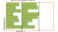
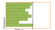
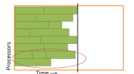
Fig. 3: Illustration of different homogeneous scheduling strategies. Left: sample synchronous homogeneous (SaSyHom); Centre: level synchronous homogeneous (LeSyHom); Right: dynamic level synchronous homogeneous (DyLeSyHom, Sec. 5.3).

Altogether $k_{\ell}^{\text{seq}}(\theta_{\ell})J_{\ell}(\theta_{\ell})\geq N_{\ell}$ samples are computed. When the run-time does not vary across samples, both strategies will results in the same MLMC run-time. If it does vary then the LeSyHom strategy has the advantage that fluctuations in the run-time $t(i,\ell,\theta)$ will be averaged and a shorter overall MLMC run-time can be expected for sufficiently large $k_{\ell}^{\text{seq}}(\theta_{\ell})$.

5.2 Run-time robust homogeneous

So far, we have assumed that the run-time is sample independent, which is idealistic (see Fig. 1, right). In the experiment in Fig. 1 (right), 3 out of 2048 samples required a run-time of $50s$ on $P_{0}^{\min}=512$ processors. On a large machine with $P_{\text{max}}=524288$ and with $\theta_{0}=0$ we need only $k_{0}^{\text{seq}}(0)=2$ sequential steps on level $0$. Therefore, the (empirical) probability that the SaSyHom strategy leads to a runtime of $100s$ is about $75\%$, while the theoretical optimal run-time is $\frac{2}{2048}\sum_{i=1}^{2048}t_{i}\approx 90s$. Here, $t_{i}$ is the actual run-time of the ith sample from Fig. 1 (right). The probability that the LeSyHom strategy leads to a runtime of $100s$ is less than $1\%$; in all other cases, a run-time of $\leq 96s$ is achieved.

Let us now fix $0\leq\ell\leq L$ again and include run-time variations in the determination of $\theta_{\ell}$. Unfortunately, in general, run-time distribution functions are not known analytically, and thus the expected run-time

$$E_{\ell,\theta}:=\mathbb{E}\left[\max_{1\leq j\leq J_{\ell}(\theta)}\Bigg{(}\sum_{k=1}^{k_{\ell}^{\text{seq}}(\theta)}t(i_{jk},\ell,\theta)\Bigg{)}\right]$$ (25)

cannot be computed explicitly. Here, the samples are denoted by $i_{jk}$ with $j=1,\ldots,J_{\ell}(\theta)$ and $k=1,\ldots,k_{\ell}^{\text{seq}}(\theta)$, related to their position in the time-processor diagram. The expression in (25) yields the actual, expected run-time on level $\ell$ to compute $J_{\ell}(\theta)k_{\ell}^{\text{seq}}(\theta)\geq N_{\ell}$ samples with $2^{3\ell+\theta}P_{0}^{\min}$ processors per sample when no synchronization after the sequential steps is performed.

The main idea is now to compute an approximation $\widehat{E}_{\ell,\theta}$ for $E_{\ell,\theta}$, and then to minimise $\widehat{E}_{\ell,\theta}$ for each $\ell$, i.e., to find $\theta_{\ell}$ such that $\widehat{E}_{\ell,\theta_{\ell}}\leq\widehat{E}_{\ell,\theta}$ for all $0\leq\theta\leq S$. As a first approximation, we replace $t(i_{jk},\ell,\theta)$ by the approximation $C_{\ell,\theta}(\omega^{i_{jk}})\,t_{\ell,\theta}$ in (20) and assume that the stochastic cost factor distribution neither depends on the level $\ell$ nor on the scale parameter $\theta$. Furthermore, we approximate the expected value by an average over $\mu$ samples to obtain the approximation

$$\widehat{E}_{\ell,\theta}(\mu):=\frac{1}{\mu}\sum_{m=1}^{\mu}\max_{1\leq j\leq J_{\ell}(\theta)}\left(\sum_{k=1}^{k_{\ell}^{\text{seq}}(\theta)}C_{0,0}(\omega^{i_{jkm}})\right)t_{\ell,\theta}\,,$$ (26)

where $i_{jkm}:=i_{jk}+(m-1)J_{\ell}(\theta)k_{\ell}^{\text{seq}}(\theta)$. If reliable data for $t_{\ell,\theta}$ is available we define

$$\theta_{\ell}:=\arg\min_{0\leq\theta\leq S}\widehat{E}_{\ell,\theta}(\mu)$$

Otherwise, we include a further approximation and replace $t_{\ell,\theta}$ by $B+2^{-\theta}(1-B)$ in (26) before finding the minimum of $\widehat{E}_{\ell,\theta}(\mu)$. Here, we still require an estimate for the serial fraction parameter $B$. To decide on the number of samples $\mu$ in (26), we keep increasing $\mu$ until it is large enough so that $\mu$ and $\mu/2$ yield the same $\theta_{\ell}$. For all our test settings, we found that $\mu\leq 500$ is sufficient.

To evaluate (26), we need some information on the stochastic cost factor $C_{0,0}(\omega)$ which was assumed to be constant across levels and across the scaling window. We use a run-time histogram associated with level $\ell=0$. This information is either available from past computations or can be built up adaptively within a MLMC method. Having the run-times $t_{k}$, $1\leq k\leq K$, of $K$ samples on level $\ell=0$ at hand, we emulate $C_{0,0}(\omega)$ by using a pseudo random integer generator from a uniform discrete distribution ranging from one to $K$ and replace the obtained value $j\leq K$ by $t_{j}K/\sum_{k=1}^{K}t_{k}$. Having computed the value of $\theta_{\ell}$, we proceed as for LeSyHom and call this strategy run-time robust homogeneous (RuRoHom). For constant run-times, RuRoHom yields again the same run-times as LeSyHom and as SaSyHom.

5.3 Dynamic variants

So far, we have used pre-computed values for $\theta_{\ell}$ and $k_{\ell}^{\text{seq}}(\theta_{\ell})$ in all variants, and each processor block carries out the computation for exactly $k_{\ell}^{\text{seq}}(\theta_{\ell})$ samples. For large run-time variations, this will still lead to unnecessary inefficiencies. Instead of assigning samples to each processor block a-priori, they can also be assigned to the processor blocks dynamically at run-time. As soon as a block terminates a computation, a new sample is assigned to it until the required number $N_{\ell}$ is reached. This reduces over-sampling and can additionally reduce the total run-time on level $\ell$. However, on massively parallel architectures this will only be efficient when the dynamic distribution of samples does not lead to a significant communication overhead. The dynamic strategy can be combined with either the LeSyHom or the RuRoHom approach and we denote them dynamic level synchronous homogeneous (DyLeSyHom) and dynamic run-time robust homogeneous (DyRuRoHom), respectively. Fig. 3 (right) illustrates the DLeSyHom strategy. Note specifically that here not all processor blocks execute the same number of sequential steps.

In order to utilize the full machine, it is crucial that no processor is blocked by actively waiting to coordinate the asynchronous execution. The necessary functionality may not be fully supported on all parallel systems. Here we use the MPI 2.0 standard that permits one-sided communication and thus allows a non-intrusive implementation. The one-sided communication is accomplished by remote direct memory access (RDMA) using registered memory windows. In our implementation, we create a window on one processor to synchronize the number of samples that are already computed. Exclusive locks are performed on a get/accumulate combination to access the number of samples.

5.4 Heterogeneous bulk synchronous scheduling

Heterogeneous strategies are clearly more flexible than homogeneous ones, but the number of scheduling possibilities grows exponentially. Thus, we must first reduce the complexity of the scheduling problem. In particular, we ignore again run-time variations and assume $t(i,\ell,\theta)=t_{\ell,\theta}$. We also assume that $N_{\ell}>0$ on all levels $\ell=0,\ldots,L$. Within an adaptive strategy, samples may only be required on some of the levels at certain times and thus this condition has to hold true only on a subset of ${\mathcal{I}}:=\{0,\ldots,L\}$.

In contrast to the homogeneous setups, we do not aim to find scaling parameters $\theta_{\ell}$ that minimize the run-time on each level separately, but instead minimize the total MLMC run-time. We formulate the minimization process as two constrained minimization steps that are coupled only in one direction, where we have to identify the number $N_{\ell,\theta}\in\mathbb{N}_{0}$ of samples on level $\ell$ which are carried out in parallel with $2^{3\ell+\theta}P_{0}^{\min}$ processors, as well as the number $k_{\ell}^{\text{seq}}(\theta)$ of associated sequential steps. Firstly, assuming $N_{\ell,\theta}$ to be given, for all $0\leq\ell\leq L$, $0\leq\theta\leq S$, we solve the constrained minimization problem for $k_{\ell}^{\text{seq}}(\theta)$

$$\arg\min_{k_{\ell}^{\text{seq}}(\theta)\in\mathbb{N}_{0}}\left(\max_{0\leq\theta\leq S}t_{\ell,\theta}\,k_{\ell}^{\text{seq}}(\theta)\right),\qquad\sum_{\theta=0}^{S}N_{\ell,\theta}\,k_{\ell}^{\text{seq}}(\theta)\geq N_{\ell}.$$

Secondly, having $k_{\ell}^{\text{seq}}(\theta)$ at hand, we find values for $N_{\ell,\theta}\in\mathbb{N}_{0}$ such as to minimize

$$\arg\min_{N_{\ell,\theta}\in\mathbb{N}_{0}}\max_{0\leq\theta\leq S\atop\,0\leq\ell\leq L}t_{\ell,\theta}k_{\ell}^{\text{seq}}(\theta),$$

the expected run-time, subject to the following inequality constraints

$$0\leq N_{\ell,\theta}\leq 2^{-3\ell}2^{-\theta}P_{\text{max}}/P_{0}^{\min},$$ (27a)

$$\sum_{\theta=0}^{S}N_{\ell,\theta}>0,\text{ for }\ell\in\mathcal{I},$$ (27b)

$$\sum_{\ell=0}^{L}\sum_{\theta=0}^{S}N_{\ell,\theta}2^{3\ell}2^{\theta}P_{0}^{\min}\leq P_{\text{max}}.$$ (27c)

We apply integer encoding [32] for the initialization and for possible mutation operators to guarantee that $N_{\ell,\theta}\in\mathbb{N}_{0}$. Clearly, if $N_{\ell,\theta}\in\mathbb{N}_{0}$ then (27c) implies (27a). However, even though it is redundant, (27a) is enforced explicitly to restrict the search space in the meta-heuristic optimization algorithm. The condition in (27b) that at least one sample is scheduled on each level at all times could also be relaxed. However, this would require a redistribution of processors in the optimization problem and can significantly increase the algorithmic and technical complexity. If (27b) is violated on some level $\ell$, we set $N_{\ell,0}=1$. Condition (27c), however, is a hard constraint. The number of processors that are scheduled cannot be larger than $P_{\text{max}}$. If (27c) is violated, we enforce it by a repeated multiplication of $N_{\ell,S},\ldots,N_{\ell,0}$ by $1/2$ until it holds. At first glance this possibly leads to an unbalanced work load, but the applied meta-heuristic search strategy compensates for it. With the values of $N_{\ell,\theta}$ identified, the samples are distributed dynamically onto the machine, see also [34].

To illustrate the complexity of this optimization task, we consider the number of different combinations for $N_{\ell,\theta}$ that satisfy (27a) but not necessarily (27b) and (27c). For example, for $L=3$, $S=4$, $P_{\text{max}}=8\,192$ and $P_{0}^{\min}=1$, there are $\mathcal{O}(10^{39})$ possible combinations. Even for the special case that the scalability window degenerates, i.e., that $S=0$, there are still $\mathcal{O}(10^{10})$ possibilities.

As an example for the following two subsections, we consider $(N_{0},N_{1},N_{2},N_{3})=(4123,688,108,16)$ and actual run-times from measurements in a set of numerical experiments:

$$(t_{\ell,\theta})_{0\leq\ell\leq 3,\atop 0\leq\theta\leq 4}=\begin{pmatrix}167&83.84&42.30&21.63&11.60\\ 171&86.28&44.53&23.13&12.41\\ 177&90.40&47.07&24.21&12.97\\ 179&91.61&48.27&24.86&13.63\end{pmatrix}.$$ (28)

5.4.1 The degenerate case $S=0$ and a new auxiliary objective

For $S=0$, a cheap but non-optimal way to choose $N_{\ell,0}$ is

$$N_{\ell,0}=\left\lfloor\frac{P_{\text{max}}\,N_{\ell}\,t_{\ell,0}}{\sum_{i=0}^{L}N_{i}2^{3i}P_{0}^{\min}t_{i,0}}\right\rfloor\,.$$ (29)

The corresponding run-time is $\max_{\ell=0,\ldots,L}t_{\ell,0}\lceil N_{\ell}/N_{\ell,0}\rceil$. The total number of processors is $\sum_{\ell=0}^{L}N_{\ell,0}2^{3\ell}P_{0}^{\min}$. This choice is acceptable when the workload is evenly distributed across levels, which is one of the typical scenarios in MLMC. It also requires that the full machine can be exploited without any imbalance in the workload.

Using the first column of (28) in (29), we find as total run-time $716\text{\,}\mathrm{s}$ and the distribution $(N_{0,0},N_{1,0},N_{2,0},N_{3,0})=(1314,221,36,5)$, see the left of Fig. 4, while on the right, the minimal run-time pattern with $684\text{\,}\mathrm{s}$ is illustrated. Due to weak scaling effects, the lower levels tend to have a larger number of sequential steps than the higher ones. We note that there exist many different configurations such that the minimal run-time is reached. Using (29) as starting guess, and then performing a local adaptive neighborhood search is much cheaper than an exhaustive search.

Fig. 4: Different scheduling patterns: Selection of $N_{\ell,0}$ by (29) (left) and optimal choice of $N_{\ell,0}$

However for $S>0$, we cannot define a good starting guess as easily and have to resort to meta-heuristic strategies. We consider simulated annealing (SA) techniques, see, e.g., [38, 40], which provide a computationally feasible approach to solve complex scheduling problems approximately. We start with $S=0$. The following experiments were performed with Python using inspyred with minor modifications. The temperature parameter in the SA method is decreased using a geometric schedule $T_{k+1}=0.8\,T_{k}$. The initial temperature is chosen to be $T_{0}=10^{3}$ which is of the order of the initial changes of the objective function.

Here we choose a Gaussian mutation with distribution $\mathcal{N}(0,0.1\,P_{\text{max}}/(2^{3\ell}P_{0}^{\min}))$ and a mutation rate of $0.2$ guaranteeing that roughly one gene per SA iteration is changed. All runs were repeated ten times with different seeds and we report minimal (min), maximal (max), as well as the arithmetically averaged (avg) MLMC run-times. Selecting $1\,000$ evaluations as the stopping criterion in SA, we obtain $t[\min,\text{avg},\max]=[684,691.2,708]\,$\mathrm{s}$$. For comparison, a stopping criterion of $2\,000$ evaluations yields $t[\min,\text{avg},\max]=[684,684,684]\,$\mathrm{s}$$. Fig. 5 shows the evolution of the average MLMC run-time between iteration 100 and 1 000 in the SA. (Please refer to the curve labelled “time [w/o aux. obj.]”). Minimizing only the run-time in the SA objective function, we observe that between iteration $250$ and iteration $800$ almost no decrease in the average run-time is achieved. This is due to the rather flat structure of the objective function in large parts of the search domain resulting from the fact that many different possible combinations yield identical run-times.

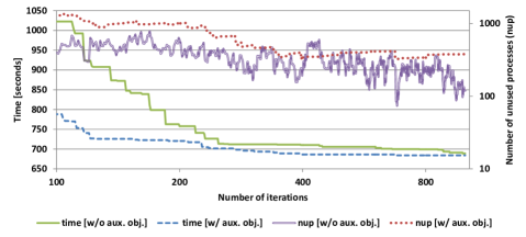
Fig. 5: Average MLMC run-time and number of unused processors (nup) with and without auxiliary objective (w/ and w/o aux. obj.) w.r.t. the number of SA iterations.

To improve the performance of the SA scheduling optimizer, we introduce the number of idle processors as a second auxiliary objective. This auxiliary objective is only considered, if two candidates result in the same MLMC run-time. In this case the candidate with the higher number of idle processors is selected. This choice is motivated by the observation that the probability to find a candidate with shorter run-time is higher in the neighborhood of a candidate that has more idle processors. Fig. 5 shows clearly that the optimization can be accelerated by including the auxiliary objective. Here, we find a MLMC run-time of less than $700\text{\,}\mathrm{s}$ in less than $300$ iterations. The optimal run-time can be obtained with $(N_{0,0},N_{1,0},N_{2,0},N_{3,0})=(1031,172,36,6)$ and a total of $7783$ processors used. From now on, we always include the number of idle processors as a secondary objective in the SA optimization algorithm.

5.4.2 The highly scalable case $S=4$ and new hybrid mutants

We use the example data in (28) and compare five different mutation operators. In addition to the already considered Gaussian mutation, we also use simpler and more sophisticated strategies. Random reset mutation replaces a gene by a uniform randomly chosen integer satisfying (27a). In the case of non-uniform mutation, see [27], a variation is added to the selected gene and the mutation depends on the SA step. The initial mutation strength is set to one and decreases with increasing iteration numbers. Tab. 1 shows that the Gaussian mutation is superior to both the random reset as well as the non-uniform mutation. However, even for the Gaussian mutation, more than $50\,000$ SA iterations are necessary to find average run-times close to the optimal one.

Table 1: Comparison of obtained MLMC run-times (min, avg, max) for different mutation operators and SA iteration numbers.

Mutation	1 000	4 000	16 000	64 000
Random reset	$627.6,676.4,772.4$	$624.6,641.0,676.8$	$627.6,633.5,659.0$	$603.9,616.4,632.8$
Non-uniform	$641.2,717.0,774.6$	$627.6,673.2,717.1$	$627.6,647.4,716.0$	$627.6,638.5,641.2$
Gaussian	$612.0,633.9,641.2$	$605.2,624.8,635.5$	$603.9,614.6,624.6$	$603.9,608.0,612.0$
Hybrid A	$624.6,632.7,641.2$	$603.9,608.0,612.0$	$604.5,604.5,604.5$	$604.5,604.5,604.5$
Hybrid B	$603.9,619.8,627.3$	$603.9,603.9,603.9$	$603.9,603.9,603.9$	$603.9,603.9,603.9$

Thus, new problem-adapted mutation operators in the SA are essential. We propose two new hybrid variants. Both perform first a Gaussian mutation and then a problem adapted mutation, taking into account the required processor numbers. The mutation rate for both is set to $0.1$.

Hybrid A: In each step, we select randomly two different “genes” $N_{\ell_{1},\theta_{1}}$ and $N_{\ell_{2},\theta_{2}}$, $0\leq\ell_{1},\ell_{2}\leq L$, $0\leq\theta_{1},\theta_{2}\leq S$, as well as a uniformly distributed random number $k\in[0,..,N_{\ell_{1},\theta_{1}}-1]$. Then we mutate

$$N_{\ell_{1},\theta_{1}}=N_{\ell_{1},\theta_{1}}-k\quad\text{and}\quad N_{\ell_{2},\theta_{2}}=N_{\ell_{2},\theta_{2}}+\left\lfloor k\,2^{\theta_{1}-\theta_{2}}2^{3(\ell_{1}-\ell_{2})}\right\rfloor.$$

If the original values for $N_{\ell_{1},\theta_{1}}$ and $N_{\ell_{2},\theta_{2}}$ were admissible, satisfying the constraints (27), then the mutated genes are also admissible. This type of mutation exploits the scalability window of the solver as well as level parallelism. For the special case $S=0$, it reduces to balancing the workload on the different levels, by exploiting the weak scalability of the solver.

Hybrid B. This variant is proposed for a PDE solver that has a large scalability window. It follows the same steps, but keeps $\ell_{1}=\ell_{2}$ fixed, therefore only exploiting the strong and weak scaling properties of the solver, but not the MLMC hierarchy.

In Tab. 1, we see that Hybrid B shows the best performance. Compared to Hybrid A it is less sensitive to the initial guess and robustly finds a very efficient scheduling scheme in less than $4\,000$ SA iterations. Thus, we restrict ourselves to SA with Hybrid B type mutations in the following examples. In the example considered in this section, it leads to the schedule

$$(N_{\ell,\theta})_{0\leq\ell\leq 3,\atop 0\leq\theta\leq 4}=\begin{pmatrix}0&443&73&0&0\\ 1&98&0&0&0\\ 0&0&3&3&0\\ 6&0&0&0&0\end{pmatrix}\quad(k_{\ell,\theta}^{\text{seq}})_{0\leq\ell\leq 3,\atop 0\leq\theta\leq 4}=\begin{pmatrix}0&7&14&0&0\\ 3&7&0&0&0\\ 0&0&12&24&0\\ 3&0&0&0&0\end{pmatrix}.$$ (30)

Comparing the two cases $S=0$ and $S=4$ shows how important the strong scalability of the solver is to reach shorter MLMC run-times. It allows to reduce the run-time by more than $10\%$, and thus the parallel MLMC performance can be improved significantly with such an advanced scheduling strategy. In the following, we call the scheduling strategy StScHet, if strong scaling is included ($S>0$). Otherwise, if no strong scaling is included ($S=0$), we call the scheduling strategy noStScHet.

To finish this section we summarise all the considered schedules in Tab. 2.

Table 2: Summary of parallel scheduling strategies.

Abbreviation	Schedule	Defined in
SaSyHom	Sample Synchronous Homogeneous	Sec. 5.1
LeSyHom	Level Synchronous Homogeneous	Sec. 5.1
RuRoHom	Run-Time Robust Homogeneous	Sec. 5.2
DyLeSyHom	Dynamic Level Synchronous Homogeneous	Sec. 5.3
DyRuRoHom	Dynamic Run-Time Robust Homogeneous	Sec. 5.3
StScHet	Heterogeneous with Strong-Scaling ($S>0$)	Sec. 5.4
noStScHet	Heterogeneous without Strong-Scaling ($S=0$)	Sec. 5.4

6 Scheduling comparison

In this section, we evaluate the sampling strategies from the previous section and illustrate the influence of the serial fraction parameter $B$, of the level-averaged number of sequential steps and of the run-time variation.

6.1 The influence of the number of sequential steps

The fact that processor and sample numbers have to be integer not only complicates the solution of the optimization problem, it also strongly influences the amount of imbalance.

Let us start with some preliminary considerations and assume that there are no run-time variations. Now, let $\Delta t\geq 0$ denote the relative difference $\Delta t$ between the run-time $\sum_{\ell=0}^{L}k_{\ell}^{\text{seq}}(\theta_{\ell})t_{\ell,\theta_{\ell}}$ of the presented homogeneous strategies and the theoretically optimal run-time in (21) (with $\mathbb{E}(C_{\ell,0})=1$). Using the MLMC level efficiency we can quantify $\Delta t$ as

$$\Delta t = \frac{P_{\text{max}}}{P_{0}^{\min}}\frac{\sum_{\ell=0}^{L}k_{\ell}^{\text{seq}}(\theta_{\ell})t_{\ell,\theta_{\ell}}}{\sum_{\ell=0}^{L}N_{\ell}2^{3\ell}t_{\ell,0}}-1=\frac{\sum_{\ell=0}^{L}N_{\ell}2^{3\ell}t_{\ell,0}(\eta_{\ell}(\theta_{\ell}))^{-1}}{\sum_{\ell=0}^{L}N_{\ell}2^{3\ell}t_{\ell,0}}-1$$

For the special case that $P_{\text{max}}/(2^{3\ell+\theta}P_{0}^{\min})\in\mathbb{N}$, we can further bound $\Delta t$ in terms of $k_{\text{seq}}:=\sum_{\ell=0}^{L}N_{\ell}2^{3\ell}P_{0}^{\min}/P_{\text{max}}$. We assume that $t_{0,0}\leq t_{0,\ell}\leq t_{0,L}$, for all $\ell=0,\ldots,L$, which is typically the case. The ratio $t_{L,0}/t_{0,0}$ reflects the weak scalability of the solver. Peta-scale aware massively parallel codes have a factor close to one. Recall from (28) that for our solver $t_{L,0}/t_{0,0}=179/167\approx 1.07$. Since $k_{\ell}^{\text{seq}}(\theta_{\ell})t_{\ell,\theta_{\ell}}\leq k_{\ell}^{\text{seq}}(0)t_{\ell,0}$ and since $k_{\ell}^{\text{seq}}(0)\leq N_{\ell}2^{3\ell}\frac{P_{0}^{\min}}{P_{\text{max}}}+1$ we have

$$\Delta t \leq \left(\frac{\max_{0\leq\ell\leq L}t_{\ell,0}}{\min_{0\leq\ell\leq L}t_{\ell,0}}\right)\frac{P_{\text{max}}}{P_{0}^{\min}}\frac{L+1}{\sum_{\ell=0}^{L}N_{\ell}2^{3\ell}}\ =\ \frac{t_{L,0}}{t_{0,0}}\,\frac{L+1}{k_{\text{seq}}}.$$

The larger $k_{\text{seq}}$, the smaller the efficiency loss.

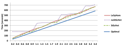
Fig. 6: Heterogeneous versus homogeneous scheduling for $k_{\text{seq}}\in[0.2,3.4]$.

In Fig. 6 we compare LeSyHom, noStScHet, StScHet and increase $k_{\text{seq}}$ from $0.2$ to $3.4$. All strategies stay within the theoretically predicted upper bound. The two scheduling strategies, LeSyHom and StScHet, that exploit the scaling properties of the solver are significantly more robust with respect to $k_{\text{seq}}$ than the heterogeneous strategy, noStScHet, for which we ignore the scalability window and set $S=0$. This observation is particularly relevant for adaptive MLMC strategies where $N_{\ell}$ may be increased within any of the adaptive steps and then a new optimal scheduling pattern has to be identified. For noStScHet, we observe a staircase pattern that is a direct consequence of the ceil operator. This effect can be easily counterbalanced by exploiting the scalability window of the solver. Moreover the run-times for LeSyHom and StScHet are larger than the optimal one by roughly a factor of $1.5$ for $k_{\text{seq}}=0.2$, but only by a factor of $1.15$ for $k_{\text{seq}}=3.4$. Thus both these strategies are robust and efficient with respect to variations in $k_{\text{seq}}$.

6.2 The influence of solver scalability

The serial fraction parameter $B$ models the strong scaling of the solver, see Sec. 5. The higher $B$, the less beneficial it is to increase $\theta$. In Fig. 7, we consider the influence of $B$ on the run-time for two different values of $k_{\text{seq}}$, namely $0.75$ and $3$, and compare LeSyHom and StScHet.

Fig. 7: Influence of the serial fraction parameter on the run-time.

First, we consider the case $k_{\text{seq}}\approx 0.75$. With a serial fraction parameter $B\leq 0.02$, there is almost no run-time difference between the two strategies. For $B$ up to $0.1$ the run-time difference is below $25\%$. However, for larger $B$, the run-time increases significantly for LeSyHom. This can be explained by the fact that for large $B$, the strong scalability property of the solver is too poor to obtain a robust scheduling pattern, and only a heterogeneous strategy with its flexibility to schedule in parallel samples on different levels can guarantee small run-times. Homogeneous strategies provide enough flexibility to be efficient in the case of large scalability windows with small values of $B$. For a small value of $k_{\text{seq}}$, the run-time of StScHet depends only very moderately on the serial fraction parameter $B$.

The situation is different for larger values of $k_{\text{seq}}$. Then both strategies exhibit roughly the same performance, but the total run-time is more sensitive to the size of $B$. A good strong scaling of the PDE solver can improve the time to solution by up to $27\%$ for the homogeneous and up to $21\%$ for the heterogeneous bulk synchronous case. As expected, carrying out one synchronization step with $k_{\text{seq}}\approx 3$ is more efficient than four steps with $k_{\text{seq}}\approx 0.75$. This observation is important for the design of efficient adaptive strategies, i.e., they should not be too fine granular. For highly performant multigrid solvers, i.e., $B\leq 0.05$, the much simpler homogeneous strategies are an excellent choice, in particular for $k_{\text{seq}}\geq 1$. On the other hand, when the parallel performance of the solver is poorer, which is typically the case in the peta-scale regime, i.e. near the strong scaling limit of the multigrid solver, the more complex heterogeneous strategies lead to significantly better efficiency gains.

6.3 Robustness and efficiency with respect to the parameters

In this subsection, we modify all three key parameters that we have discussed so far. We assume again that the run-time variations $C_{\ell,\theta}(\cdot)$ are independent of $\ell$ and $\theta$ and use a half-normal distribution to model $C_{0,0}(\cdot)$. More specifically, we assume that $C_{0,0}(\cdot)-1$ follows a half-normal distribution with parameter Var, i.e. its mode is at 1. The time $t_{\ell,\theta}$ is chosen to be the run-time of the mode, as described in Sec. 4.1.

Fig. 8: MLMC efficiencies for different values of the parameters $k_{\text{seq}}$, $B$ and Var, and for all the different scheduling strategies.

Fig. 8 illustrates the parallel efficiencies of all the strategies developed above (cf. Tab. 2), as well as their robustness with respect to the parameters $k_{\text{seq}}$, $B$ and Var,. The parallel efficiency is calculated with respect to the theoretical, optimal run-times given in (21) not with actual measured run-times. We choose $B\in\{0.01,0.1,1\}$ and $\textit{Var}\in\{0,0.5,2\}$, and set the sample numbers on the different levels to be $(N_{0},N_{1},N_{2},N_{3})=k_{\text{seq}}(1366,228,36,5)$, with $k_{\text{seq}}\in\{0.98,4.92,23.60\}$ (abbreviated by $\{1,5,24\}$ in Fig. 8).

We comment first on the case of no run-time variations, i.e., $\!\textit{Var}\!=0$, where our numerical results confirm that all homogeneous strategies produce the same performance. For large numbers of sequential steps, the homogeneous variants are superior to the heterogeneous ones. This is mainly due to the constraint (27b) which forces us to consider all levels in parallel. As mentioned above, this constraint is not essential and dropping it might lead to more efficient heterogeneous strategies. This will be the subject of future work. If variations in the run-time are included, then all homogeneous strategies yield different results. The parallel efficiency of the simplest one, SaSyHom, then drops to somewhere between $0.1$ and $0.55$. As expected, the worst performance is observed for a small $k_{\text{seq}}$, poor solver scalability, and high run-time variation. In that case, the dynamic variants can counterbalance the run-time variations more readily and provide computationally inexpensive scheduling schemes (provided the technical realization is feasible).

Secondly, we discuss the case of a small value of $k_{\text{seq}}$. This typically occurs if the machine is large or if the adaptive MLMC algorithm is used. Here, only the heterogeneous strategies can guarantee acceptable parallel efficiencies for all values of $B$. The homogeneous variants result in efficiencies below $0.7$ and $0.4$, for $\textit{Var}=0$ and for $B=0.1$ and $B=1$, respectively.

In all considered cases, one of our strategies results in parallel efficiencies of more than $0.5$; in many cases even more than $0.7$. For moderate run-time variations and large enough $k_{\text{seq}}$, the parallel efficiency of StScHet improves to more than $0.8$. StScHet is also the most robust strategy with respect to solver scalability. However, for solvers with good scalability, i.e. $B\leq 0.05$, the DyRoRuHom strategy is an attractive alternative, since it does not require any sophisticated meta-heuristic scheduling algorithm and can dynamically adapt to run-time variations in the samples.

7 Numerical results for MLMC

In this section, the scheduling strategies developed above are employed in a large-scale MLMC computation. We consider the model problem in Sec. 3 with $D=(0,1)^{3}$ and $f\equiv 1$, discretised by piecewise linear FEs. For the relevant problem sizes, the serial fraction parameter for our multigrid PDE solver is $B\leq 0.02$, and the fluctuations in run-time are $<2\%$. Only few timings deviate substantially from the average (c.f. Fig. 1) so that we focus on investigating strategies for that regime.

The following experiments were carried out on the peta-scale supercomputer JUQUEEN, a 28 rack BlueGene/Q system located in Jülich, Germany. Each of the 28 672 nodes has 16 GB main memory and 16 cores operating at a clock rate of 1.6 GHz. The compute nodes are connected via a five-dimensional torus network. HHG is compiled by the IBM XL C/C++ Blue Gene/Q, V12.0 compiler suite with MPICH2 that implements the MPI-2 standard and supports RDMA. Four hardware threads can be used on each core to hide latencies. We always use 2 processes (threads) per core to maximize the execution efficiency.

7.1 Static scheduling for scenarios with small run-time variations

We choose four MLMC levels, i.e., $L=3$, with a fine grid that has roughly $1.1\cdot 10^{9}$ mesh nodes. The random coefficient is assumed to be lognormal with exponential covariance, $\sigma^{2}=1$ and $\lambda=0.02$. The quantity of interest is the PDE solution $u$ evaluated at the point $x=(0.25,0.25,0.25)$. All samples are computed using a fixed multigrid cycle structure with one FMG-2V(4,4) cycle, i.e., a full multigrid method (nested iteration) with two V-cycles per new level, as well as four pre- and four post-smoothing steps. In [19] it is shown that this multigrid method delivers the solution of a scalar PDE with excellent numerical and parallel efficiency. In particular, the example is designed such that after completing the FMG-2V(4,4) cycle for all samples, the minimal and maximal residual differ at most by a factor $1.5$ within each MLMC level. For the MLMC estimator, an a priori strategy is assumed, based on pre-computed variance estimates, such that $(N_{\ell})_{\ell=1,2,3,4}=(4\,123,688,108,16)$. We first study the balance between sample and solver parallelism and thus the tradeoffs between the efficiency of the parallel solver and possible load imbalances in the sampling strategy, as introduced in Sec. 4.1. We set $P_{0}^{\text{min}}=1$, and consequently $P_{\ell}^{\text{min}}=2^{3\ell}$. The run-times to compute a single sample with $P_{\ell}^{\text{min}}$ processors are measured as $(t_{\ell,0})_{\ell=0,1,2,3}=(166,168,174,177)$ seconds, showing only a moderate increase in runtime and confirming the excellent performance of the multigrid solver.

A lower bound for the run-time of the parallel MLMC estimator of $t^{\text{opt}}_{\text{mlmc}}=520\,$\mathrm{s}$$ is now provided by eq. (21). A static cost model is justified since the timings between individual samples vary little. We therefore employ the level synchronous homogeneous (LeSyHom) scheduling strategy, as introduced in Sect. 5.1. This requires only a few, cheap real time measurements to configure the MLMC scheduling strategy. The smaller $\theta$, the larger the solver efficiency $\text{Eff}_{\ell}(\theta)$while the larger $\theta$, the smaller $\text{Imb}_{\ell}(\theta)$. To study this effect quantitatively, we measure the parallel solver efficiency. Here, we do not use (22), but actual measured values for $t_{\ell,\theta}$ instead, and we find that on level $\ell=0$ we have $\{\text{Eff}_{0}(0),\text{Eff}_{0}(1),\text{Eff}_{0}(2),\text{Eff}_{0}(3),\text{Eff}_{0}(4)\}=\{1,0.99,0.96,0.92,0.86\}$.

In Tab. 3, we present for each level the efficiency $\eta_{\ell}(\theta)$, see (24), and the run-time as a function of $\theta$. For $\theta=0$ and $\ell=0$, the runs are carried out with one thread, and they go up to 8 192 hardware threads on 4 096 cores for $\theta=4$ and $\ell=3$. We see a very good correlation between predicted efficiencies and actual measured times in Tab. 3. The maximal efficiency and the minimal run-time on each level are marked in boldface to highlight the best setting.

Table 3: Level and total run-time and efficiency of MLMC for fixed $\theta$.

$\theta$	time	$\eta_{0}(\theta)$	time	$\eta_{1}(\theta)$	time	$\eta_{2}(\theta)$	time	$\eta_{3}(\theta)$	time	$\eta(\theta)$
0	167	0.50	171	0.67	177	0.84	179	1.00	694	0.75
1	168	0.50	173	0.67	181	0.84	183	0.99	704	0.74
2	127	0.64	134	0.86	188	0.81	193	0.96	642	0.81
3	108	0.74	139	0.83	169	0.89	199	0.92	615	0.85
4	104	0.77	136	0.84	181	0.81	218	0.86	640	0.83

Keeping $\theta$ fixed, the minimal run-time is $615$. Our homogeneous scheduling strategies pick $\theta_{\ell}$ for each level automatically and by doing so, a considerably shorter run-time of $586$ is obtained, increasing the efficiency to $0.89$. If it were possible to scale the solver perfectly also to processor numbers that are not necessarily powers of 2, we could reduce the compute time even further by about $11\%$ from $586$ to $520$ seconds. In summary, we see that exploiting the strong scaling of the PDE solver helps to avoid load imbalances due to oversampling and improves the time to solution by about $15\%$ from $694$ to $586$ seconds. The cost is well distributed across all levels, although most of the work is on the finest level which is typical for this model problem (cf. [4]).

We conclude this subsection with a strong scaling experiment, i.e., we increase the number of processes in order to reduce the overall time to solution. Since we are interested to analyse the behavior for extremely large $P_{\text{max}}$, we reduce the number of samples to $N_{l}=(1\,031,172,27,4)$. The time for one MLMC computation with an increasing number of processes $P_{\text{max}}$ is presented in Fig. 9.

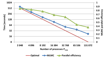
Fig. 9: Strong scaling of MLMC using homogeneous bulk synchronous scheduling.

The initial computation employs $P_{\text{max}}=2\,048$ which is large enough so that all fine-grid samples can be computed concurrently. We scale the problem up to 131 072 processes. Increasing $P_{\text{max}}$ while keepimg the number of samples per level fixed results in a decrease of $k_{\text{seq}}$. Thus the load imbalance increases and the total parallel efficiency decreases. Nevertheles even with $P_{\text{max}}=32768$, we obtain a parallel efficiency over $60\%$ while for $P_{\text{max}}=131072$ the eficiency drops below $40\%$. This can be circumvented by an increase of the size $S$ of the sclability window. Overall the compute time for the MLMC estimator can be reduced from $616$ to $22$ seconds. For each choice of $P_{\text{max}}$, we select the optimal regime for $\theta_{\ell}$, $\ell=0,\ldots,3$, as discussed above. Together with the excellent strong scaling behavior of the parallel HHG multigrid solver this leads to the here demonstrated combined parallel efficiency of the MLMC implementation.

7.2 Adaptive MLMC

Finally, we consider an adaptive MLMC algorithm as introduced in Sec. 2.3 in a weak scaling scenario, i.e., increasing the problem size proportionally to the processor count.

Table 4: Weak scaling of an adaptive MLMC estimator.

			No. Samples		Correlation	Idle
Processes	Resolution	Runtime	Fine	Total	length	time
4 096	$1\,024^{3}$	$5.0\cdot 10^{3}$ s	68	13 316	1.50E-02	3%
32 768	$2\,048^{3}$	$3.9\cdot 10^{3}$ s	44	10 892	7.50E-03	4%
262 144	$4\,096^{3}$	$5.2\cdot 10^{3}$ s	60	10 940	3.75E-03	5%

Table 5: Number of samples and over-samples for different levels for the largest run.

		No. Samples		No. Over-samples
Level	No. partitions	Scheduled	Calculated	Estimated	Actual
0	2 048	7 506	8 192	3 726	686
1	256	2 111	2 304	429	193
2	32	382	384	15	2
3	4	57	60	3	3

Each row in Tab. 5 summarizes one adaptive MLMC computation. The MLMC method is initially executed on 2 048 cores and $P_{\ell}$ is chosen as $P_{\ell=1,2,3,4}=(2,16,128,1\,024)$, In each successive row of the table, the number of unknowns on the finest level in MLMC and the number of processors on each level is increased by a factor of eight. Moreover, the correlation length $\lambda$ of the coefficient field is reduced by a factor of two ($\sigma^{2}=1$ is kept fixed). This means that the problems are actually getting more difficult as well. The quantity of interest is defined as the flux across a separating plane $\Gamma$ at $x_{2}=0.25$, i.e.,

$$Q(u,\omega)=\int_{\Gamma}k(x,\omega)\frac{\partial u}{\partial n}ds\,.$$

In all cases, the initial number of samples is set to $N_{\ell=1,2,3,4}=(1\,024,256,64,16)$. The final number of samples is then chosen adaptively by the MLMC algorithm. It is listed in the table. As motivated in Sec. 2, the tolerance for the sampling error, which is needed in (15) to adaptively estimate $N_{\ell}$, is chosen as $\varepsilon_{s}\approx|\mathbb{E}[Q_{L}-Q_{L-1}]|$, balancing the sampling error with the bias error.

Fig. 10: MLMC performance plots: expected value (left) and variance (right) of $Q_{\ell}$ (red, solid) and $Y_{\ell}$ (blue, dashed) for $\lambda=0.015$ and $\sigma^{2}=1$.

The estimates for the expected values and for the variances of $Q_{\ell}$ and $Y_{\ell}$, for a problem of size $M_{\ell}=1\,024^{3}$ and with a correlation length of $\lambda=0.015$, are plotted in Fig. 10. The expected values and the variances of $Y_{\ell}$ show the expected asymptotic behavior as $\ell$ increases, confirming the benefits of the multilevel approach. The total number of samples that are computed is 13 316, but only 68 of them on the finest grid. A standard Monte Carlo estimator would require several thousand samples on level 3 and would be significantly more costly. The idle time, in the last column of Tab. 5, accounts for the variation in the number of V-cycles, required to achieve a residual reduction of $10^{-5}$ on each level within each call to the FMG multigrid algorithm.

The largest adaptive MLMC computation shown in Tab. 5 involves a finest grid with almost $7\text{\times}{10}^{10}$ unknowns. Discrete systems of this size must be solved $60$ times, together with more than 10 000 smaller problems, the smallest of which still has more than $1.6\text{\times}{10}^{7}$ unknowns. With the methods developed here, a computation of such magnitude requires a compute time of less than 1.5 hours when 131 072 cores running 262 144 processes are employed. Additional details for this largest MLMC computation are presented in Tab. 5. The table lists the number of partitions that are used on each level for the respective problem sizes. The number of calculated samples on each level is a multiple of the number of these partitions. As Tab. 5 illustrates, the number of scheduled samples is smaller and the difference indicates the amount of oversampling. The number of unnecessary samples is presented explicitly in the last column of the table to compare with the estimated number of unneeded samples. This estimated number is significantly higher on each level, since it is the sum of all the oversampled computations in all stages of the adaptive MLMC algorithm. As we pointed out earlier, this is caused by a special feature of the adaptive MLMC algorithm. Samples that were predicted to be redundant in an early stage of the algorithm, may become necessary later in the computation. Thus at termination, the actual oversampling is significantly less than predicted. This is a dynamic effect that cannot be quantified easily in a static a priori fashion.

8 Conclusions

In this paper we have explored the use of multilevel Monte Carlo methods on very large supercomputers. Three levels of parallelism must be coordinated, since it is not sufficient to just execute samples in parallel. The combination of solver- and sample-parallelism leads to a non-trivial scheduling problem, where the trade-off between solver scalability, oversampling, and additional efficiency losses due to run-time variations must be balanced with care. This motivated the development of scheduling strategies of increasing complexity, including advanced dynamic methods that rely on meta-heuristic search algorithms. These scheduling algorithms are based on performance predictions for the individual tasks that can in turn be derived from run-time measurements and performance models motivated by Amdahl’s law.

The success of the techniques and their scalability are demonstrated on a large-scale model problem. The largest MLMC computation involves more than 10 000 samples and a fine grid resolution with almost $7\text{\times}{10}^{10}$ unknowns. It is executed on 131 072 cores of a peta-scale class supercomputer in 1.5 hours of total compute time.

References

- [1] A. H. Baker, R. D. Falgout, T. Gamblin, T. V. Kolev, M. Schulz, and U. M. Yang. Scaling algebraic multigrid solvers: On the road to exascale. In Competence in High Performance Computing 2010, pages 215–226. Springer, 2012.
- [2] A. Barth, C. Schwab, and N. Zollinger. Multi-level Monte Carlo finite element method for elliptic PDE’s with stochastic coefficients. Numer. Math., 119:123–161, 2011.
- [3] B. K. Bergen and F. Hülsemann. Hierarchical hybrid grids: data structures and core algorithms for multigrid. Numer. Lin. Alg. Appl., 11(2-3):279–291, 2004.
- [4] J. Charrier, R. Scheichl, and A. L. Teckentrup. Finite element error analysis of elliptic PDEs with random coefficients and its application to multilevel Monte Carlo methods. SIAM J. Numer. Anal., 51(1):322–352, 2013.
- [5] E. Chow, R. D. Falgout, J. J. Hu, R. S. Tuminaro, and U. M. Yang. A survey of parallelization techniques for multigrid solvers. In M. A. Heroux, P. Raghavan, and H. D. Simon, editors, Parallel Processing for Scientific Computing, chapter 10, pages 179–201. SIAM, 2006.
- [6] K. A. Cliffe, M. B. Giles, R. Scheichl, and A. L. Teckentrup. Multilevel Monte Carlo methods and applications to elliptic PDEs with random coefficients. Comput. Visual. Sci., 14(1):3–15, 2011.
- [7] N. Collier, A. L. Haji-Ali, F. Nobile, E. von Schwerin, and R. Tempone. A continuation multilevel Monte Carlo algorithm. BIT Numer. Math., 55(2):399–432, 2015.
- [8] C. R. Dietrich and G. H. Newsam. Fast and exact simulation of stationary Gaussian processes through circulant embedding of the covariance matrix. SIAM J. Sci. Comput., 18:1088–1107, 1997.
- [9] J. Dongarra. Report on the Sunway TaihuLight system. Technical report, University of Tennessee, Oak Ridge National Laboratory, June 24, 2016. http://www.netlib.org/utk/people/JackDongarra/PAPERS/sunway-report-2016.pdf.
- [10] M. Drozdowski. Scheduling for Parallel Processing. Springer-Verlag, London, 2009.
- [11] D. Elfverson, F. Hellman, and A. Målqvist. A multilevel Monte Carlo method for computing failure probabilities. SIAM/ASA J. Uncertainty Quantification, 4(1):312–330, 2016.
- [12] M. Garey and D. Johnson. Computers and Intractability; A Guide to the Theory of NP-Completeness. W. H. Freeman Co, New York, 1990.
- [13] R. G. Ghanem and P. Spanos. Stochastic Finite Elements: A Spectral Approach. Springer, 1991.
- [14] M. B. Giles. Multilevel Monte Carlo path simulation. Operations Res., 56(3):981–986, 2008.
- [15] M. B. Giles and B. J. Waterhouse. Multilevel quasi-Monte Carlo path simulation. Radon Series Comp. Appl. Math., 8:1–18, 2009.
- [16] B. Gmeiner, M. Huber, L. John, U. Rüde, and B. Wohlmuth. A quantitative performance study for stokes solvers at the extreme scale. J. Comput. Sci., 2016. Accepted for publication.
- [17] B. Gmeiner, H. Köstler, M. Stürmer, and U. Rüde. Parallel multigrid on hierarchical hybrid grids: a performance study on current high performance computing clusters. Concurrency and Computation: Practice and Experience, 26(1):217–240, 2014.
- [18] B. Gmeiner, U. Rüde, H. Stengel, C. Waluga, and B. Wohlmuth. Performance and scalability of hierarchical hybrid multigrid solvers for Stokes systems. SIAM J. Sci. Comput., 37(2):C143–C168, 2015.
- [19] B. Gmeiner, U. Rüde, H. Stengel, C. Waluga, and B. Wohlmuth. Towards textbook efficiency for parallel multigrid. Numer. Math. Theor. Meth. Appl., 8(01):22–46, 2015.
- [20] I. G. Graham, F. Y. Kuo, D. Nuyens, R. Scheichl, and I. H. Sloan. Quasi-Monte Carlo methods for elliptic PDEs with random coefficients and applications. J. Comput. Phys., 230:3668–3694, 2011.
- [21] G. Hager and G. Wellein. Introduction to high performance computing for scientists and engineers. CRC Press, 2010.
- [22] V. H. Hoang, C. Schwab, and A. M. Stuart. Complexity analysis of accelerated MCMC methods for Bayesian inversion. Inverse Prob., 29:085010, 2013.
- [23] J. K. Lenstra, A. H. G. Rinnooy Kan, and P. Brucker. Complexity of machine scheduling. Annals of Discrete Mathematics, 1:343–362, 1977.
- [24] J. L. Leva. A fast normal random number generator. ACM Transactions on Mathematical Software (TOMS), 18(4):449–453, 1992.
- [25] F. Lindgren, H. Rue, and J. Lindström. An explicit link between gaussian fields and gaussian markov random fields: the stochastic partial differential equation approach. Journal of the Royal Statistical Society: Series B (Statistical Methodology), 73(4):423–498, 2011.
- [26] G. J. Lord, C. Powell, and T. Shardlow. An Introduction to Computational Stochastic PDEs. Cambridge Texts in Applied Mathematics. Cambridge University Press, 2014.
- [27] Z. Michalewicz. Genetic Algorithms Data Structures Evolution Programs. Springer, 1996.
- [28] S. Mishra, C. Schwab, and J. Šukys. Multi-level Monte Carlo finite volume methods for shallow water equations with uncertain topography in multi-dimensions. SIAM J. Sci. Comput., 34:761–784, 2012.
- [29] R. Potsepaev and C. L. Farmer. Application of stochastic partial differential equations to reservoir property modelling. page B003. ECMOR XII, 2010.
- [30] W. H. Press. Numerical Recipes 3rd Edition: The Art of Scientific Computing. Cambridge University Press, 2007.
- [31] D. Simpson, J. Illian, F. Lindgren, S. Sørbye, and H. Rue. Going off grid: Computationally efficient inference for log-Gaussian Cox processes. Biometrika, 103:49–70, 2016.
- [32] M. Srinivas and L. M. Patnaik. Genetic algorithms: A survey. Computer, 27(6):17–26, 1994.
- [33] E. Strohmaier, H. W. Meuer, J. Dongarra, and H. D. Simon. The Top500 list and progress in high-performance computing. Computer, 48(11):42–49, 2015.
- [34] J. Šukys. Adaptive load balancing for massively parallel multi-level Monte Carlo solvers. In Parallel Processing and Applied Mathematics, pages 47–56. Springer, 2014.
- [35] J. Šukys, S. Mishra, and C. Schwab. Static load balancing for multi-level Monte Carlo finite volume solvers. In Parallel Processing and Applied Maths, pages 245–254. Springer, 2012.
- [36] A. L. Teckentrup, R. Scheichl, M. B. Giles, and E. Ullmann. Further analysis of multilevel MC methods for elliptic PDEs with random coefficients. Numer. Math., 125(3):569–600, 2013.
- [37] J. D. Ullman. NP-complete scheduling problems. J. Comput. System Sci., 10:384–393, 1975.
- [38] P. J. M. Van Laarhoven and E. H. L. Aarts. Simulated annealing. Springer, 1987.
- [39] P. J. M. Van Laarhoven, E. H. L. Aarts, and J. K. Lenstra. Job shop scheduling by simulated annealing. Operations Res., 40(1):113–125, 1992.
- [40] I. Wegener. Simulated annealing beats Metropolis in combinatorial optimization. In L. Caires et al., editors, Automata, Languages and Programming, volume 3850 of Lecture Notes in Computer Science, pages 589–601. Springer, 2005.
- [41] P. Whittle. Stochastic processes in several dimensions. Bull. Inst. Internat. Stat., 40:974–994, 1963.
- [42] D. Xiu and G. E. Karniadakis. The Wiener–Askey polynomial chaos for stochastic differential equations. SIAM J. Sci. Comput., 24(2):619–644, 2002.