Saturation scale fluctuations and multi-particle rapidity correlations

Abstract

We study the effect of intrinsic fluctuations of the proton saturation momentum scale on event-by-event rapidity distributions. Saturation scale fluctuations generate an asymmetry in the single particle rapidity distribution in each event resulting in genuine $n$-particle correlations having a component linear in the rapidities of the produced particles, $y_{1}\cdots y_{n}$. We introduce a color domain model that naturally explains the centrality dependence of the two-particle rapidity correlations recently measured by ATLAS Aaboud et al. (2016) while constraining the probability distribution of saturation scale fluctuations in the proton. Predictions for $n=4,6$ and $8$ particle correlations find that the four- and eight-particle cumulant change sign at an intermediate multiplicity, a signature which could be tested experimentally.

I Introduction

An outstanding challenge within the field of relativistic heavy-ion collisions is understanding the apparent collective behavior seen in smaller colliding systems ranging from p+p Khachatryan et al. (2016); Aad et al. (2016), p+Pb Aad et al. (2013); Abelev et al. (2013a); Chatrchyan et al. (2013), d+Au Adare et al. (2015a) to ³He$+$Au Adare et al. (2015b). For a review both on the experimental and theoretical situation we refer the reader to Dusling et al. (2016a).

This is in contrast to larger system sizes, such as those produced in more-central Au+Au and Pb+Pb collisions, where a hydrodynamic treatment may be argued to be appropriate. The measured momentum-space azimuthal anisotropies, when confronted with hydrodynamic simulations, provide detailed information on the transport properties of the system and strong constrains on differing initial state treatments Heinz and Snellings (2013).

What remains unclear is whether the hydrodynamic paradigm is also applicable to smaller colliding systems as well. Or whether the observed anisotropies are evidence for alternative sources of collectivity, such as multi-gluon correlations already embedded in the colliding wavefunctions Dumitru et al. (2011). What is clear, is that a first principles understanding of the initial state fluctuations will be necessary to unravel the situation.

The focus of this work will be on multi-particle rapidity correlations. Just as spatial inhomogeneities in the transverse plane can be converted into azimuthal momentum-space correlation, longitudinal shape fluctuations can also be converted into momentum-space rapidity correlations Bzdak and Teaney (2013). This new facet can provide further insight into the nature of event-by-event fluctuations, see, e.g, Broniowski and Bożek (2016), in particular those responsible for the highest multiplicity classes corresponding to rare configurations of the proton.

Suppose in each event the single particle rapidity distribution is asymmetric in rapidity. Statistical fluctuations could in principle generate such an asymmetry, however, these are eliminated by measuring correlation functions. Instead we will focus on dynamical fluctuations produced at the onset of the collision; for example by a disparity in the left- and right-going constituents or local fluctuations in the color charge density in the projectile and target. Regardless of the physical mechanism the event-by-event single particle distribution can be characterized by a series in rapidity,

$$\frac{dN}{dy}=\left\langle\frac{dN}{dy}\right\rangle\left(1+a_{0}+a_{1}y+\ldots\right)\,,$$ (1)

where $\left\langle dN/dy\right\rangle$ is the event-averaged single particle distribution. By construction we therefore have $\langle a_{i}\rangle=0$ and in order to access the event-by-event fluctuations encoded in the $a_{i}$ one must look at multi-particle correlations. For example, the two-particle correlation function $C_{2}$ reads Bzdak and Teaney (2013)

$$\frac{C_{2}(y_{1},y_{2})}{\left\langle dN/dy_{1}\right\rangle\left\langle dN/dy_{2}\right\rangle}=\left\langle a_{0}^{2}\right\rangle+\left\langle a_{0}a_{1}\right\rangle\left(y_{1}+y_{2}\right)+\left\langle a_{1}^{2}\right\rangle y_{1}y_{2}+\cdots\,,$$ (2)

where

$$C_{2}(y_{1},y_{2})\equiv\left\langle\frac{d^{2}N}{dy_{1}dy_{2}}\right\rangle-\left\langle\frac{dN}{dy_{1}}\right\rangle\left\langle\frac{dN}{dy_{2}}\right\rangle\,.$$ (3)

By measuring $C_{2}$ one is able to access the root-mean-squared event-by-event fluctuations of $a_{i}$. This work will focus on the leading term $\left<a_{1}^{2}\right>$ (the term $\left<a_{0}^{2}\right>$ is related to usual multiplicity fluctuations within an event class and is of no interest to the present analysis, and $\left<a_{0}a_{1}\right>=0$ for symmetric collisions). More details can be found in Bzdak and Teaney (2013) and Jia et al. (2016).

In a similar fashion $n$-particle correlation functions, $C_{n}(y_{1},...,y_{n})$, closely related to the $n$-particle cumulants can be calculated. The correlation function $C_{n}(y_{1},...,y_{n})$ as defined measures genuine $n$-particle correlations by subtracting correlations acting between fewer than $n$ particles. This process is described in appendix A. Here we write down the main expressions necessary for this work. The leading component of the $n$-particle correlation, $C_{n}$, is given by Bzdak and Bozek (2016)

$$\frac{C_{n}(y_{1},...,y_{n})}{\left\langle dN/dy_{1}\right\rangle\cdots\left\langle dN/dy_{n}\right\rangle}=\left\langle a_{1}^{n}\right\rangle_{[n]}y_{1}\cdots y_{n}\,+\cdots\,,$$ (4)

where ${\left\langle a_{1}^{2}\right\rangle}_{[2]}\equiv{\left\langle a_{1}^{2}\right\rangle}$, as in equation 2, and

$${\left\langle a_{1}^{4}\right\rangle}_{[4]} = {\left\langle a_{1}^{4}\right\rangle}-3{\left\langle a_{1}^{2}\right\rangle}^{2}\,,$$ (5)

$${\left\langle a_{1}^{6}\right\rangle}_{[6]} = {\left\langle a_{1}^{6}\right\rangle}-15{\left\langle a_{1}^{2}\right\rangle}{\left\langle a_{1}^{4}\right\rangle}+30{\left\langle a_{1}^{2}\right\rangle}^{3}\,,$$ (6)

$${\left\langle a_{1}^{8}\right\rangle}_{[8]} = {\left\langle a_{1}^{8}\right\rangle}-28{\left\langle a_{1}^{2}\right\rangle}{\left\langle a_{1}^{6}\right\rangle}-35{\left\langle a_{1}^{4}\right\rangle}^{2}+420{\left\langle a_{1}^{2}\right\rangle}^{2}{\left\langle a_{1}^{4}\right\rangle}-630{\left\langle a_{1}^{2}\right\rangle}^{4}\,.$$ (7)

The subscript $[n]$ denotes that the object is related to a genuine $n$-particle correlation. For symmetric collisions, such as p+p, the correlation function is symmetric in rapidity $C_{n}(y_{1},...,y_{n})=C_{n}(-y_{1},...,-y_{n})$ and therefore $\langle a_{1}^{n}\rangle=0$ for $n=1,3,5,\cdots$.

The event-by-event fluctuations we will be interested in arise from gluon number fluctuations in the high-energy evolution of QCD. In the Color Glass Condensate framework Gelis et al. (2010) the small-$x$ hadronic wavefunction evolves according to the B-JIMWLK Iancu et al. (2001); Jalilian-Marian et al. (1997, 1998) renormalization group equation. In a mean-field approximation the B-JIMWLK hierachy reduces to a single non-linear evolution equation, the Balitsky-Kovchegov (BK) equation Kovchegov (2000); Balitsky (1996). While the BK equation serves as a good approximation to dipole evolution when the occupation number is large compared to one, it was recognized Mueller and Shoshi (2004); Iancu et al. (2005) that that discreteness due to the finite number of partons in a given event can lead to an appreciable effect on physical observables.

A generalization of the B-JIMWLK hierarchy was derived in Iancu and Triantafyllopoulos (2005a, b) to take into account gluon number fluctuations. This hierarchy reduces (after coarse-graining in impact parameter space) to the BK equation supplemented with a stochastic noise term. The main consequence of the noise term is to introduce dispersion in the saturation scale event-by-event (as observed in numerical simulations of the Langevin BK equation Soyez (2005)). The saturation scale can be treated as a random variable drawn from a probability distribution having cumulants derived in the context of a stochastic reaction diffusion model Brunet et al. (2006) which at asymptotically high energies takes the form Marquet et al. (2006),

$$P[\rho]=\frac{1}{\sqrt{2\pi}\sigma}\exp\left(-\frac{\rho^{2}}{2\sigma^{2}}\right)\,,\;\;\;\rho\equiv\ln\left(\frac{Q^{2}}{\bar{Q}^{2}}\right)\,.$$ (8)

The variance $\sigma^{2}=\alpha_{s}N_{c}/\pi DY$ is proportional to $D$, the dispersion coefficient of the wavefronts, and the amount of evolution in $Y$. In this work we will treat $\sigma$ as energy-independent parameter, fixed for LHC energies. If looking at correlations over a large range of beam energies or kinematic conditions then the evolution of $\sigma$ would need to be considered.

The importance of fluctuations beyond those present in the conventional CGC framework has already been recognized. For example, in Schenke et al. (2014) fluctuations due to the impact parameter of the collision along with sub-nucleonic color charge fluctuations as implemented in the IP-Glasma model are unable to explain the tail of the multiplicity distribution in p+p collisions. As a second example we point out that in order to obtain a quantitative description of the ridge-like correlations of high multiplicity p+p collisions the proton must fluctuate such that its effective saturation scale is 5-6 times its minimum bias value Dusling et al. (2016b).

It was shown more recently that saturation scale fluctuations of the form given in equation 8 can help explain the charged particle pseudo-rapidity distributions in p+A collisions McLerran and Praszalowicz (2016) and reconcile the tail of the multiplicity distribution in p+p collisions McLerran and Tribedy (2016) finding values of $\sigma\sim 1.5$ and $\sigma\sim 0.5$ respectively.

In a previous work, reference Bzdak and Dusling (2016), we evaluated $C_{2}(y_{1},y_{2})$ in p+p collisions from saturation scale fluctuations on an event-by-event basis drawn from the above distribution. The KLN model Kharzeev and Levin (2001); Kharzeev et al. (2005); Kharzeev and Nardi (2001) for the single particle multiplicity, that has successfully accounted for the bulk multiplicity in heavy-ion collisions (see Abelev et al. (2013b); Adam et al. (2016) for recent examples at the highest LHC energies), was used to compute the asymmetric component of the two-particle correlation function for minimum bias p+p collisions. These results showed that

$$\langle a_{1}^{2}\rangle\simeq\frac{1}{2}\lambda^{2}\sigma^{2}$$ (9)

in the limit of small $\sigma$ (the full expression for any $\sigma$ can be found in Bzdak and Dusling (2016) and is rederived in section II). The parameter $\lambda$ quantifies the rapidity dependence of the saturation scale due to quantum evolution

$$Q^{2}=Q_{o}^{2}e^{-\lambda y}$$ (10)

and has been constrained to the range $0.25\lesssim\lambda\lesssim 0.35$ by phenomenological fits of deep inelastic scattering data at small-$x$ Golec-Biernat and Wusthoff (1998); Praszalowicz and Stebel (2013); Praszałowicz and Francuz (2015). From this constraint on $\lambda$ we concluded that a value of $\sigma\sim 0.5-1$ is consistent with the recent ATLAS measurement The ATLAS collaboration (2015) of $\sqrt{{\left\langle a_{1}^{2}\right\rangle}}\approx 0.1$ in minimum-bias p+p collisions.

In this work we extend our study beyond two-particle correlations and find a closed form expression for the $n-$particle correlation function. The full result is worked out in section II but for small sigma and even $n$ we find

$$\left<a_{1}^{n}\right>\simeq\left(\lambda\sigma\right)^{n}\left[\frac{n!}{2^{n}(n/2)!}-\frac{n(n/2)!}{\sqrt{\pi}}\sigma+\cdots\right]\,,$$ (11)

and the cumulants defined in equations 5-7 can be calculated accordingly

$${\left\langle a_{1}^{2}\right\rangle}_{[2]}\simeq\frac{\lambda^{2}\sigma^{2}}{2}\,,\;\;\;{\left\langle a_{1}^{4}\right\rangle}_{[4]}\simeq-\frac{2\lambda^{4}\sigma^{5}}{\sqrt{\pi}}\,,\;\;\;{\left\langle a_{1}^{6}\right\rangle}_{[6]}\simeq\frac{3\lambda^{6}\sigma^{7}}{2\sqrt{\pi}}\,,\;\;\;{\left\langle a_{1}^{8}\right\rangle}_{[8]}\simeq-\frac{3\lambda^{8}\sigma^{9}}{\sqrt{\pi}}\,.$$ (12)

While the second order cumulant goes as $\sigma^{2}$ it is worth noting that the leading $\sigma^{n}$ behavior of the n’th order cumulants vanish from the subtraction of the disconnected pieces and the leading behavior becomes $\sigma^{n+1}$ for $n\geq 4$.

In section III we introduce a color domain model which explains the centrality dependence of $\left<a_{1}^{n}\right>$ through the centrality dependence of the variance, $\sigma$, of saturation scale fluctuations. In essence we argue along the same lines of Dumitru et al. (2008) that correlated particle production occurs within domains of size $Q_{s}^{-2}$. The saturation scale fluctuates independently in each domain and therefore fluctuations in the impact parameter averaged (effective) saturation scale will be suppressed by the number of domains. As the multiplicity scales with the number of domains we expect that $\sigma^{2}\sim 1/N_{\rm ch}$. This argument naturally explains the ATLAS data The ATLAS collaboration (2015) which observes that $\sqrt{\left<a_{1}^{2}\right>}\sim 1/N_{\rm ch}^{0.5}$.

We should emphasize that this is not the first work to propose the use of rapidity correlations to probe the nature of the hadronic wave-function. For example, it was shown in Gelis et al. (2009); Dusling et al. (2010) that when the rapidity separation between two particles is larger than $1/\alpha_{s}$ the two-particle rapidity distribution is sensitive to the QCD evolution in the hadronic wavefunctions of the projectile and target. For symmetric colliding systems, such as p+p or Pb+Pb, the event-averaged distribution can be asymmetric if the triggered particles have different transverse momenta. Particles of different momenta experience a differing amounts of small-$x$ evolution and therefore decorrelate with rapidity at different speeds. However, after integrating over transverse momenta a symmetric rapidity distribution is recovered.

II Multi-particle correlations

Following our previous paper Bzdak and Dusling (2016), we will derive a general expression for the $n$-particle cumulant. Our starting point is the KLN expression  Kharzeev and Levin (2001); Kharzeev et al. (2005); Kharzeev and Nardi (2001) for single inclusive production

$$\frac{dN}{dy}\propto S_{\perp}\mathrm{Min}[Q_{1}^{2},Q_{2}^{2}]\left(2+\ln\frac{\mathrm{Max}[Q_{1}^{2},Q_{2}^{2}]}{\mathrm{Min}[Q_{1}^{2},Q_{2}^{2}]}\right)\,,$$ (13)

with the two saturation scales of each colliding ion represented by $Q_{1}$ and $Q_{2}$, both of which evolve with rapidity according to

$$Q_{1}^{2}=Q_{o,1}^{2}e^{+\lambda y}\,,\,\,\,Q_{2}^{2}=Q_{o,2}^{2}e^{-\lambda y},$$ (14)

were $Q_{o,1}$ and $Q_{o,2}$ are the initial saturation scales at $y=0$. The parameter $\lambda$ describes the growth of the gluon structure function at small-$x$. It is precisely this parameter, capturing quantum corrections to the classical gluon dynamics, responsible for deviations from a purely boost-invariant (i.e. rapidity independent) spectra. The expression used above for the multiplicity is valid away from the fragmentation region.

The wave-function of each colliding hadron fluctuates independently on an event-by-event basis. Our goal is to study the consequence of independent fluctuations of $Q_{o,1}$ and $Q_{o,2}$ drawn from an appropriate distribution. This work will focus exclusively on the log-normal distribution motivated by studies of Langevin BK equation discussed earlier; refinements on this choice could be study for future work. Recapitulating, the saturation scale fluctuates according to the log-normal distribution,

$$P[\rho]=\frac{1}{\sqrt{2\pi}\sigma}\exp\left[-\frac{\rho^{2}}{2\sigma^{2}}\right]\,,\,\,\,\mathrm{where}\,\,\,\,\rho\equiv\ln\left(\frac{Q^{2}}{\bar{Q}^{2}}\right)\,.$$ (15)

The expectation value of observables are computed from

$$\left\langle\mathcal{O}\right\rangle=\int_{-\infty}^{+\infty}d{\rho_{1}}d{\rho_{2}}P[{\rho_{1}}]P[{\rho_{2}}]\;\mathcal{O}[{\rho_{1}},{\rho_{2}}]\,.$$ (16)

For example, the mean saturation scale $\left\langle Q\right\rangle$, is related to $\bar{Q}$ through $\left\langle Q\right\rangle=\bar{Q}\exp(\sigma^{2}/8)$, and therefore take $\left\langle Q\right\rangle\simeq\bar{Q}$ for $\sigma\ll 1$. In this paper we consider symmetric p+p collision and thus $\bar{Q}_{o,1}^{2}=\bar{Q}_{o,2}^{2}\equiv\bar{Q}_{o}^{2}$.

Defining the variables $\rho_{1,2}$ for each nucleus

$${\rho_{1}}\equiv\ln\frac{Q_{o,1}^{2}}{\bar{Q}_{o}^{\>2}}\,,\,\,\,{\rho_{2}}\equiv\ln\frac{Q_{o,2}^{2}}{\bar{Q}_{o}^{\>2}}\,,$$ (17)

we can re-express equation 13 as,

$$\frac{1}{S_{\perp}\bar{Q}_{o}^{2}}\frac{dN}{dy}\propto\begin{cases}e^{{\rho_{1}}+\lambda y}\left(2+{\rho_{2}}-{\rho_{1}}-2\lambda y\right),&\mbox{if }2\lambda y<{\rho_{2}}-{\rho_{1}}\\ e^{{\rho_{2}}-\lambda y}\left(2+{\rho_{1}}-{\rho_{2}}+2\lambda y\right),&\mbox{if }2\lambda y\geq{\rho_{2}}-{\rho_{1}}\end{cases}$$ (18)

The expectation value of the multiplicity can be evaluated in closed form,

$$\frac{1}{S_{\perp}\bar{Q}_{o}^{2}}\left\langle\frac{dN}{dy}\right\rangle = \frac{\sigma}{\sqrt{\pi}}\exp\left[\frac{\sigma^{2}}{4}-\frac{\lambda^{2}y^{2}}{\sigma^{2}}\right]+\left(1+\lambda y-\frac{\sigma^{2}}{2}\right)\exp\left[\frac{\sigma^{2}}{2}-\lambda y\right]\mathrm{Erfc}\left[\frac{\sigma}{2}-\frac{\lambda y}{\sigma}\right]$$ (19)

$$+ \left\{y\to-y\right\}$$

where $\mathrm{Erfc}$ is the complementary error function. Using the above equations we can expand $\frac{dN/dy}{\langle dN/dy\rangle}$ in $y$, see Eq. (1), and extract the $a_{1}$ coefficient for fixed $\rho_{1}$ and $\rho_{2}$,

$$a_{1}\left[\rho_{1},\rho_{2}\right]=\frac{\lambda\sqrt{\pi}\exp\left(-\frac{\sigma^{2}}{2}\right)\left(\rho_{1}-\rho_{2}\right)\left\{\exp(\rho_{1})-\left[\exp(\rho_{1})-\exp(\rho_{2})\right]\mathrm{H}\left(\rho_{1}-\rho_{2}\right)\right\}}{\sqrt{\pi}(\sigma^{2}-2)\mathrm{Erfc}\left(\frac{\sigma}{2}\right)-2\sigma\exp\left(-\frac{\sigma^{2}}{4}\right)}$$ (20)

where $\mathrm{H}$ is the Heaviside step function. Note that $a_{1}\left[\rho_{1},\rho_{2}\right]=0$ for $\rho_{1}=\rho_{2}$ since in this case there is no asymmetry. Taking the expectation value (as defined in equation 16) of the $n$-th power of the above expression results in,

$$\left\langle a_{1}^{n}\right\rangle=\frac{\left[\lambda\sigma\sqrt{\pi}\exp\left(\frac{\sigma^{2}\left(n-2\right)}{4}\right)\right]^{n}}{\sqrt{\pi}}\frac{n!\mathrm{U}\left(\frac{1+n}{2};\frac{1}{2};\frac{n^{2}\sigma^{2}}{4}\right)}{\left[\sqrt{\pi}(\sigma^{2}-2)\mathrm{Erfc}\left(\frac{\sigma}{2}\right)-2\sigma\exp\left(-\frac{\sigma^{2}}{4}\right)\right]^{n}}\,,$$ (21)

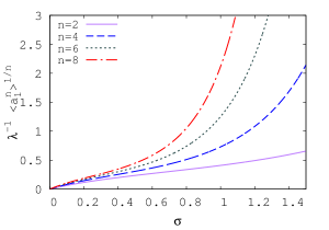
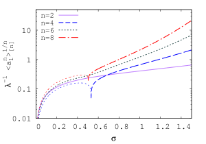
where $\mathrm{U}$ is the confluent hypergeometric function. Figure 1 shows $\lambda^{-1}{\left\langle a_{1}^{n}\right\rangle}^{1/n}$ and $\lambda^{-1}{\left\langle a_{1}^{n}\right\rangle}^{1/n}_{[n]}$ as a function of $\sigma$ for $n=2,4,6,8$. For ${\left\langle a_{1}^{4}\right\rangle}$ and ${\left\langle a_{1}^{8}\right\rangle}$ the cumulant becomes negative for $\sigma\lesssim 0.5$ (independent of $\lambda$). This sign change in ${\left\langle a_{1}^{4}\right\rangle}_{[4]}$ and ${\left\langle a_{1}^{8}\right\rangle}_{[8]}$ is not entirely unexpected; it is a consequence of the relative strength of the intrinsic $n$-particle correlation from disconnected lower order contributions. A similar sign change is seen in the four-particle azimuthal cumulant which becomes negative for $N_{\rm trk}\gtrsim 40$ Khachatryan et al. (2015). In the following section we will introduce a simple color domain model relating $\sigma^{2}$ to the multiplicity.

Figure 1: Left: Equation 21 plotted as a function of $\sigma$ for $n=2,4,6,8$. Right: Cumulants as defined in equations  5-7 for $n=2,4,6,8$. For $n=4$ and $n=8$ when the cumulant is negative ($\sigma\lesssim 0.5$) we take the absolute value and plot it as the dashed curve.

III Color domain model

A first principle consideration of gluon number fluctuations are well beyond the scope of this work. As discussed in detail in Iancu and Triantafyllopoulos (2005b); Mueller et al. (2005) extending the B-JIMWLK hierarchy to include gluon number fluctuations with impact parameter dependence results in a stochastic equation having mathematical proprieties not fully understood.

In order to make phenomenological progress, we introduce a simple model to capture the centrality dependence of $\sigma$–the variance of saturation scale fluctuations. Consider the proton in the high-energy limit of QCD at moderate value of $x$ such that the McLerran-Venugopalan McLerran and Venugopalan (1994a, b, c) model may serve as a good first approximation to the gluon dynamics of the nuclear wavefunction. The semi-classical small-$x$ gluon fields are sourced by large-$x$ valence partons treated as recoilless random color charges. The created small-$x$ field has a correlation length $1/Q_{s}$, where $Q_{s}$ is the typical transverse momentum of the gluons. We therefore assume that saturation scale fluctuations occur independently in color domains of size $1/Q_{s}$.

We picture the proton as having $N_{\rm d}$ color domains, with the saturation scale of each domain fluctuating independently according to a log-normal probability distribution of the form 8. If we identify $\bar{Q}_{\rm d}$ as the mean saturation scale of each color domain and $\sigma_{\rm d}^{2}$ as the variance of fluctuations around the average one can generate a new probability distribution for the saturation scale fluctuations of the nucleus as a whole.

While there is no known analytic expression for the probability distribution resulting from a sum over independently fluctuating log-normal random variables it can be approximated by another log-normal Fenton (1960); Cobb et al. (2012) having the following variance and mean,

$$\sigma^{2} =\ln\left[\frac{1}{N_{\rm d}}\left(e^{\sigma_{\rm d}^{2}}-1\right)+1\right]\,,$$ (22)

$$\ln\left(\bar{Q}_{o}^{2}\right) =\ln\left(\bar{Q}_{\rm d}^{2}\right)+\frac{1}{4}\left(\sigma_{\rm d}^{2}-\sigma^{2}\right)\,.$$ (23)

It will be instructive to look at the above result in the limit of small $\sigma$. For weak fluctuations we have $\bar{Q}_{o}=\bar{Q}_{\rm d}$, expressing the fact that the transverse spatially averaged saturation scale is equivalent to the average saturation scale of the domains. Furthermore, for weak fluctuations the variance scales with the number of domains as

$$\sigma^{2}\approx\frac{\sigma_{\rm d}^{2}}{N_{\rm d}}.$$ (24)

This is the expected result for a normally distributed random variable, which the log-normal approximates for small values of the variance. Given the qualitative nature of the discussion we will use the small $\sigma$ approximation given in equation 24 moving forward.

It was recognized Lappi and McLerran (2006) that the classical fields following the collisions of two saturated nuclei consists of approximately boost-invariant longitudinal chromo-electric and -magnetic fields of transverse size $Q_{s}^{-2}$. Each flux tube emits approximately $1/\alpha_{s}$ gluons. A collision having overlap area $S_{\perp}$ therefore has $N_{\rm ft}\equiv(S_{\perp}Q_{s}^{2})$ fluxtubes and a total multiplicity, $N_{\rm ch}\sim 1/\alpha_{s}(S_{\perp}Q_{s}^{2})$. Under the reasonable assumption that the number of fluxtubes scales with the number of color domains in the nucleus $N_{\rm ft}\sim N_{\rm d}$ we see that correlated particle production occurs within a flux tube and the correlation strength is suppressed by $1/N_{\rm ft}$, similar in spirit to the flux-tube interpretation of the near-side ridge put forth in Dumitru et al. (2008).

Based on the above considerations we can express the multiplicity dependence of $\sigma$ to its value in minimum bias (mb) collisions through

$$\sigma^{2}=\frac{N_{\rm ch}^{\rm mb}}{N_{\rm ch}}\sigma_{\rm mb}^{2}\,.$$ (25)

where $N_{\rm ch}^{\rm mb}$ is the minimum bias charged particle multiplicity.

We will study two values of $\lambda=0.25$ and $0.35$ covering the allowed range in phenomenological fits of Deep Inelastic Scattering data at small-$x$ Golec-Biernat and Wusthoff (1998); Praszalowicz and Stebel (2013); Praszałowicz and Francuz (2015). In figure 2 we show the centrality dependence of $\sqrt{\left\langle a_{1}^{2}\right\rangle}$ computed from equation 21 where $\sigma$ is a function of the charged particle multiplicity $N_{\rm ch}$ through equation 25 where we use the ATLAS value of $N_{\rm ch}^{\rm mb}=17.6$. The minimum bias variance, $\sigma_{\rm mb}$ is fit to the minimum bias data as done in our previous work Bzdak and Dusling (2016).

Figure 2: $\langle a_{1}^{2}\rangle^{1/2}$ as a function of $N_{\rm ch}$ compared to preliminary data in p+p collisions by the ATLAS collaboration The ATLAS collaboration (2015). For comparison we also show the preliminary data in p+Pb and Pb+Pb interactions.

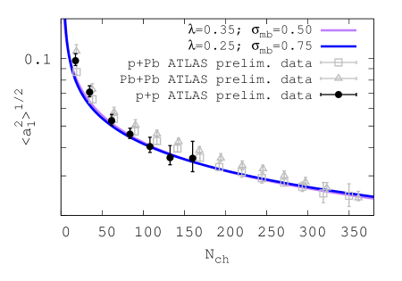
The agreement with data is rather striking given the single parameter fit. The parameter $\lambda$ is tightly constrained by both numerical simulations of QCD evolution and phenomenological fits to data. The free parameter $\sigma_{\rm mb}$ could in principle have taken on any value but happens to fall in the range of the other approaches constraining it McLerran and Praszalowicz (2016); McLerran and Tribedy (2016). While one could argue that the $N_{\rm ch}^{1/2}$ dependence of the data could have fallen out of any independent cluster model, see, e.g, Broniowski and Bożek (2016), the overall strength of the correlation is sensitive to the specific physics input that generates the correlation.

The similarity between the p+p, p+Pb and Pb+Pb experimental data may be suggestive of a similar underlying particle production mechanism, however there is no reason apriori to expect them to agree at this level. In p+Pb and Pb+Pb collisions one expects nucleonic fluctuations to have a sizable effect as shown for example in Schenke and Schlichting (2016).

Figure 3: Left: $10^{4}{\left\langle a_{1}^{4}\right\rangle}_{[4]}$ as a function of charged particle multiplicity, $N_{\rm ch}$. Right: $\sqrt[1/4]{-{{\left\langle a_{1}^{4}\right\rangle}}_{[4]}}$, $\sqrt[1/6]{{{\left\langle a_{1}^{6}\right\rangle}}_{[6]}}$, $\sqrt[1/8]{-{{\left\langle a_{1}^{8}\right\rangle}}_{[8]}}$ as a function of charged particle multiplicity, $N_{\rm ch}$.

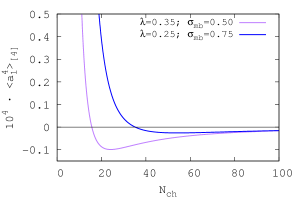
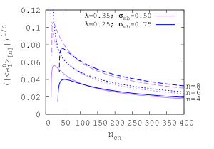
Figure 3 shows predictions for the higher order cumulants as a function of $N_{\rm ch}$. In the left plot we show $10^{4}{\left\langle a_{1}^{4}\right\rangle}_{[4]}$ as a function of $N_{\rm ch}$ for the same parameters successfully able to reproduce the two-particle correlation. At low multiplicity the cumulant is dominated by the intrinsic four-particle correlation while at higher multiplicity lower order intrinsic correlations dominate in the subtraction specified in equation 5 making the cumulant negative.

In the right plot we present $\sqrt[1/4]{-{{\left\langle a_{1}^{4}\right\rangle}}_{[4]}}$, $\sqrt[1/6]{{{\left\langle a_{1}^{6}\right\rangle}}_{[6]}}$, $\sqrt[1/8]{-{{\left\langle a_{1}^{8}\right\rangle}}_{[8]}}$ at higher multiplicity where the above quantities are real. For large multiplicities, where $\sigma$ is small, we have the following analytic expressions,

$$\sqrt[1/n]{|{\left\langle a_{1}^{n}\right\rangle}_{[n]}|}\approx\lambda\left(\sigma_{\rm mb}^{2}\frac{N_{\rm ch}^{\rm mb}}{N_{\rm ch}}\right)^{\frac{n+1}{2n}}\,,$$ (26)

for the $n=4,6,8$ cumulant. A measurement of the above quantity could tightly constraint the nature of the fluctuations used in this model.

IV Conclusions

In conclusion, we calculated and discussed multi-particle correlation functions in rapidity originating from the fluctuating saturation scales in proton-proton collisions.

The difference between the left- and right-going proton saturation scales on an event-by-event basis naturally lead to a rapidity asymmetry and consequently nontrivial long-range rapidity correlations. We focused on the first non-trivial asymmetric component, ${\left\langle a_{1}^{n}\right\rangle}_{[n]}y_{1}\cdots y_{n}$ and provided compact analytical expression for the cumulants ${\left\langle a_{1}^{n}\right\rangle}_{[n]}$.

Introducing a simple color domain model we argued that the variance, $\sigma$, of saturation scale fluctuations is suppressed at higher multiplicities as $\sigma\sim N_{\rm ch}^{-0.5}$, a consequence that higher multiplicity collisions necessarily contain a larger number of independently fluctuating domains.

We found a satisfactory agreement between the experimentally measured ${\left\langle a_{1}^{2}\right\rangle}$ and our model and made predictions for higher order cumulants. At high multiplicities we find that the quantities ${\left\langle a_{1}^{4}\right\rangle}_{[4]}$ and ${\left\langle a_{1}^{8}\right\rangle}_{[8]}$ change sign to negative values; a feature which could be tested in future experiments.

We hope that this work will spur future investigations in this direction. Studying the partonic structure and accessing the Wigner distribution of the proton has been the impetus for many deep inelastic scattering experiments but have mostly been limited to a minimum bias proton. The experimental study of proton fluctuations has been largely limited. See Mäntysaari and Schenke (2016) for a recent proposal to access these type of fluctuations in incoherent diffraction processes. Our work provides another route to access information on the proton’s structure in ultra-rare configurations.

Acknowledgments:

AB was supported by the Ministry of Science and Higher Education (MNiSW), by founding from the Foundation for Polish Science, and by the National Science Centre, Grant No. DEC-2014/15/B/ST2/00175, and in part by DEC-2013/09/B/ST2/00497.

Appendix A Cumulants

By definition the genuine $n$-particle correlation function, $C_{n}(y_{1},...,y_{n})$, also known as the $n$-particle cumulant, is different than zero only if there is an explicit correlation between $n$ or more particles. For example, for three particles we have

$$C_{3}(y_{1},y_{2},y_{3}) = \left\langle\frac{d^{3}N}{dy_{1}dy_{2}dy_{3}}\right\rangle-\left\langle\frac{dN}{dy_{1}}\right\rangle\left\langle\frac{dN}{dy_{2}}\right\rangle\left\langle\frac{dN}{dy_{3}}\right\rangle-$$ (27)

$$\left\langle\frac{dN}{dy_{1}}\right\rangle C_{2}(y_{2},y_{3})-\left\langle\frac{dN}{dy_{2}}\right\rangle C_{2}(y_{1},y_{3})-\left\langle\frac{dN}{dy_{3}}\right\rangle C_{2}(y_{1},y_{2}),$$

where $C_{2}$ is the two-particle correlation function, equation 3. For four particles the formula is a bit more complex

$$C_{4} = \left\langle\frac{d^{4}N}{dy_{1}dy_{2}dy_{3}dy_{4}}\right\rangle-\left\langle\frac{dN}{dy_{1}}\right\rangle\left\langle\frac{dN}{dy_{2}}\right\rangle\left\langle\frac{dN}{dy_{3}}\right\rangle\left\langle\frac{dN}{dy_{4}}\right\rangle-$$ (28)

$$\underset{6}{\underbrace{\left\langle\frac{dN}{dy_{i}}\right\rangle\left\langle\frac{dN}{dy_{j}}\right\rangle C_{2}(y_{k},y_{l})}}-\underset{4}{\underbrace{\left\langle\frac{dN}{dy_{i}}\right\rangle C_{3}(y_{j},y_{k},y_{l})}}-\underset{3}{\underbrace{C_{2}(y_{i},y_{j})C_{2}(y_{k},y_{l})}},$$

where the numbered braces show the number of possible variations. The explicit expressions for up to six particles can be found in Bzdak and Bozek (2016) and the general formula for an arbitrary number of particles in Botet and Ploszajczak (2002).

The $n$-particle densities, $\left\langle\frac{d^{n}N}{dy_{1}\cdots dy_{n}}\right\rangle$ can be readily expressed through the ${\left\langle a_{1}^{k}\right\rangle}$ terms, for example

$$\frac{\left\langle\frac{d^{4}N}{dy_{1}\cdots dy_{4}}\right\rangle}{\left\langle\frac{dN}{dy_{1}}\right\rangle\cdots\left\langle\frac{dN}{dy_{4}}\right\rangle} = \left\langle\left(1+a_{1}y_{1}\right)\left(1+a_{1}y_{2}\right)\left(1+a_{1}y_{3}\right)\left(1+a_{1}y_{4}\right)\right\rangle$$ (29)

$$= 1+{\left\langle a_{1}^{2}\right\rangle}\left(y_{1}y_{2}+\ldots+y_{3}y_{4}\right)+{\left\langle a_{1}^{4}\right\rangle}y_{1}y_{2}y_{3}y_{4},$$

where for clarity we keep only the $a_{1}$ term and take ${\left\langle a_{1}\right\rangle}={\left\langle a_{1}^{3}\right\rangle}=0$. The genuine $n$-particle correlation function can be expressed by the ${\left\langle a_{1}^{k}\right\rangle}$ terms. For example for four particles we obtain

$$\frac{C_{4}(y_{1},...,y_{4})}{\left\langle dN/dy_{1}\right\rangle\cdots\left\langle dN/dy_{4}\right\rangle}={\left\langle a_{1}^{4}\right\rangle}_{[4]}y_{1}y_{2}y_{3}y_{4}+...$$ (30)

where ${\left\langle a_{1}^{4}\right\rangle}_{[4]}={\left\langle a_{1}^{4}\right\rangle}-3{\left\langle a_{1}^{2}\right\rangle}^{2}$.

References

- Aaboud et al. (2016) M. Aaboud et al. (ATLAS), (2016), arXiv:1606.08170 [hep-ex] .
- Khachatryan et al. (2016) V. Khachatryan et al. (CMS), Phys. Rev. Lett. 116, 172302 (2016), arXiv:1510.03068 [nucl-ex] .
- Aad et al. (2016) G. Aad et al. (ATLAS), Phys. Rev. Lett. 116, 172301 (2016), arXiv:1509.04776 [hep-ex] .
- Aad et al. (2013) G. Aad et al. (ATLAS Collaboration), Phys.Rev.Lett. 110, 182302 (2013), arXiv:1212.5198 [hep-ex] .
- Abelev et al. (2013a) B. Abelev et al. (ALICE Collaboration), Phys.Lett. B719, 29 (2013a), arXiv:1212.2001 [nucl-ex] .
- Chatrchyan et al. (2013) S. Chatrchyan et al. (CMS Collaboration), Phys.Lett. B718, 795 (2013), arXiv:1210.5482 [nucl-ex] .
- Adare et al. (2015a) A. Adare et al. (PHENIX), Phys. Rev. Lett. 114, 192301 (2015a), arXiv:1404.7461 [nucl-ex] .
- Adare et al. (2015b) A. Adare et al. (PHENIX), Phys. Rev. Lett. 115, 142301 (2015b), arXiv:1507.06273 [nucl-ex] .
- Dusling et al. (2016a) K. Dusling, W. Li, and B. Schenke, Int. J. Mod. Phys. E25, 1630002 (2016a), arXiv:1509.07939 [nucl-ex] .
- Heinz and Snellings (2013) U. Heinz and R. Snellings, Ann. Rev. Nucl. Part. Sci. 63, 123 (2013), arXiv:1301.2826 [nucl-th] .
- Dumitru et al. (2011) A. Dumitru, K. Dusling, F. Gelis, J. Jalilian-Marian, T. Lappi, et al., Phys.Lett. B697, 21 (2011), arXiv:1009.5295 [hep-ph] .
- Bzdak and Teaney (2013) A. Bzdak and D. Teaney, Phys. Rev. C87, 024906 (2013), arXiv:1210.1965 [nucl-th] .
- Broniowski and Bożek (2016) W. Broniowski and P. Bożek, Phys. Rev. C93, 064910 (2016), arXiv:1512.01945 [nucl-th] .
- Jia et al. (2016) J. Jia, S. Radhakrishnan, and M. Zhou, Phys. Rev. C93, 044905 (2016), arXiv:1506.03496 [nucl-th] .
- Bzdak and Bozek (2016) A. Bzdak and P. Bozek, Phys. Rev. C93, 024903 (2016), arXiv:1509.02967 [hep-ph] .
- Gelis et al. (2010) F. Gelis, E. Iancu, J. Jalilian-Marian, and R. Venugopalan, Ann.Rev.Nucl.Part.Sci. 60, 463 (2010), arXiv:1002.0333 [hep-ph] .
- Iancu et al. (2001) E. Iancu, A. Leonidov, and L. D. McLerran, Nucl. Phys. A692, 583 (2001), arXiv:hep-ph/0011241 [hep-ph] .
- Jalilian-Marian et al. (1997) J. Jalilian-Marian, A. Kovner, A. Leonidov, and H. Weigert, Nucl. Phys. B504, 415 (1997), arXiv:hep-ph/9701284 [hep-ph] .
- Jalilian-Marian et al. (1998) J. Jalilian-Marian, A. Kovner, A. Leonidov, and H. Weigert, Phys. Rev. D59, 014014 (1998), arXiv:hep-ph/9706377 [hep-ph] .
- Kovchegov (2000) Y. V. Kovchegov, Phys. Rev. D61, 074018 (2000), arXiv:hep-ph/9905214 [hep-ph] .
- Balitsky (1996) I. Balitsky, Nucl. Phys. B463, 99 (1996), arXiv:hep-ph/9509348 [hep-ph] .
- Mueller and Shoshi (2004) A. H. Mueller and A. I. Shoshi, Nucl. Phys. B692, 175 (2004), arXiv:hep-ph/0402193 [hep-ph] .
- Iancu et al. (2005) E. Iancu, A. H. Mueller, and S. Munier, Phys. Lett. B606, 342 (2005), arXiv:hep-ph/0410018 [hep-ph] .
- Iancu and Triantafyllopoulos (2005a) E. Iancu and D. N. Triantafyllopoulos, Nucl. Phys. A756, 419 (2005a), arXiv:hep-ph/0411405 [hep-ph] .
- Iancu and Triantafyllopoulos (2005b) E. Iancu and D. N. Triantafyllopoulos, Phys. Lett. B610, 253 (2005b), arXiv:hep-ph/0501193 [hep-ph] .
- Soyez (2005) G. Soyez, Phys. Rev. D72, 016007 (2005), arXiv:hep-ph/0504129 [hep-ph] .
- Brunet et al. (2006) E. Brunet, B. Derrida, A. H. Mueller, and S. Munier, Phys. Rev. E73, 056126 (2006), arXiv:cond-mat/0512021 [cond-mat] .
- Marquet et al. (2006) C. Marquet, G. Soyez, and B.-W. Xiao, Phys. Lett. B639, 635 (2006), arXiv:hep-ph/0606233 [hep-ph] .
- Schenke et al. (2014) B. Schenke, P. Tribedy, and R. Venugopalan, Phys. Rev. C89, 024901 (2014), arXiv:1311.3636 [hep-ph] .
- Dusling et al. (2016b) K. Dusling, P. Tribedy, and R. Venugopalan, Phys. Rev. D93, 014034 (2016b), arXiv:1509.04410 [hep-ph] .
- McLerran and Praszalowicz (2016) L. McLerran and M. Praszalowicz, Annals Phys. 372, 215 (2016), arXiv:1507.05976 [hep-ph] .
- McLerran and Tribedy (2016) L. McLerran and P. Tribedy, Nucl. Phys. A945, 216 (2016), arXiv:1508.03292 [hep-ph] .
- Bzdak and Dusling (2016) A. Bzdak and K. Dusling, Phys. Rev. C93, 031901 (2016), arXiv:1511.03620 [hep-ph] .
- Kharzeev and Levin (2001) D. Kharzeev and E. Levin, Phys. Lett. B523, 79 (2001), arXiv:nucl-th/0108006 [nucl-th] .
- Kharzeev et al. (2005) D. Kharzeev, E. Levin, and M. Nardi, Phys. Rev. C71, 054903 (2005), arXiv:hep-ph/0111315 [hep-ph] .
- Kharzeev and Nardi (2001) D. Kharzeev and M. Nardi, Phys. Lett. B507, 121 (2001), arXiv:nucl-th/0012025 [nucl-th] .
- Abelev et al. (2013b) B. Abelev et al. (ALICE), Phys. Rev. Lett. 110, 032301 (2013b), arXiv:1210.3615 [nucl-ex] .
- Adam et al. (2016) J. Adam et al. (ALICE), Phys. Rev. Lett. 116, 222302 (2016), arXiv:1512.06104 [nucl-ex] .
- Golec-Biernat and Wusthoff (1998) K. J. Golec-Biernat and M. Wusthoff, Phys. Rev. D59, 014017 (1998), arXiv:hep-ph/9807513 [hep-ph] .
- Praszalowicz and Stebel (2013) M. Praszalowicz and T. Stebel, JHEP 03, 090 (2013), arXiv:1211.5305 [hep-ph] .
- Praszałowicz and Francuz (2015) M. Praszałowicz and A. Francuz, Phys. Rev. D92, 074036 (2015), arXiv:1507.08186 [hep-ph] .
- The ATLAS collaboration (2015) The ATLAS collaboration, ATLAS-CONF-2015-051 (2015).
- Dumitru et al. (2008) A. Dumitru, F. Gelis, L. McLerran, and R. Venugopalan, Nucl.Phys. A810, 91 (2008), arXiv:0804.3858 [hep-ph] .
- Gelis et al. (2009) F. Gelis, T. Lappi, and R. Venugopalan, Phys. Rev. D79, 094017 (2009), arXiv:0810.4829 [hep-ph] .
- Dusling et al. (2010) K. Dusling, F. Gelis, T. Lappi, and R. Venugopalan, Nucl.Phys. A836, 159 (2010), arXiv:0911.2720 [hep-ph] .
- Khachatryan et al. (2015) V. Khachatryan et al. (CMS), Phys. Rev. Lett. 115, 012301 (2015), arXiv:1502.05382 [nucl-ex] .
- Mueller et al. (2005) A. H. Mueller, A. I. Shoshi, and S. M. H. Wong, Nucl. Phys. B715, 440 (2005), arXiv:hep-ph/0501088 [hep-ph] .
- McLerran and Venugopalan (1994a) L. D. McLerran and R. Venugopalan, Phys. Rev. D49, 2233 (1994a), arXiv:hep-ph/9309289 [hep-ph] .
- McLerran and Venugopalan (1994b) L. D. McLerran and R. Venugopalan, Phys. Rev. D49, 3352 (1994b), arXiv:hep-ph/9311205 [hep-ph] .
- McLerran and Venugopalan (1994c) L. D. McLerran and R. Venugopalan, Phys. Rev. D50, 2225 (1994c), arXiv:hep-ph/9402335 [hep-ph] .
- Fenton (1960) L. Fenton, IRE Transactions on Communications Systems 8, 57 (1960).
- Cobb et al. (2012) B. R. Cobb, R. Rumı, and A. Salmerón, Statistics and Computing 16, 293 (2012).
- Lappi and McLerran (2006) T. Lappi and L. McLerran, Nucl. Phys. A772, 200 (2006), arXiv:hep-ph/0602189 [hep-ph] .
- Schenke and Schlichting (2016) B. Schenke and S. Schlichting, (2016), arXiv:1605.07158 [hep-ph] .
- Mäntysaari and Schenke (2016) H. Mäntysaari and B. Schenke, (2016), arXiv:1603.04349 [hep-ph] .
- Botet and Ploszajczak (2002) R. Botet and M. Ploszajczak, Universal fluctuations: The phenomenology of hadronic matter (2002).