Intervalley scattering of graphene massless Dirac fermions at 3-periodic grain boundaries

Abstract

We study how low-energy charge carriers scatter off periodic and linear graphene grain boundaries oriented along the zigzag direction with a periodicity three times greater than that of pristine graphene. These defects map the two Dirac points into the same position, and thus allow for intervalley scattering to occur. Starting from graphene’s first-neighbor tight-binding model we show how can we compute the boundary condition seen by graphene’s massless Dirac fermions at such grain boundaries. We illustrate this procedure for the 3-periodic pentagon-only grain boundary, and then work out the low-energy electronic scattering off this linear defect. We also compute the effective generalized potential seen by the Dirac fermions at the grain boundary region.

I Introduction

Chemical vapor deposition (CVD) of graphene on metal surfacesLi et al. (2009); Reina et al. (2009); Kim et al. (2009); Bae et al. (2010) is currently viewed as one of the most promising scalable methods for economically producing large and abundant high-quality monolayer graphene sheets. It is thus greatly important to fully understand and control the behavior of electrons on this form of graphene.

CVD graphene, as any other solid grown by chemical vapor deposition, is generally a polycrystal composed by several grains with distinct crystallographic orientations. These grains are separated by grain boundaries (GBs),Meyer et al. (2008); Lahiri et al. (2010); Huang et al. (2011); Kim et al. (2011); Nemes-Incze et al. (2011); Ophus et al. (2015) which due to the $sp^{2}$ bonding structure of carbon atoms in graphene, are typically made of pentagonal, heptagonal and octagonal rings of carbon atoms.Meyer et al. (2008); Lahiri et al. (2010); Huang et al. (2011); Kim et al. (2011); Ophus et al. (2015) Grain boundaries generally intercept each other at random angles, being neither periodic nor perfect straight lines.

The properties of CVD graphene flakes are strongly influenced by the quantity, distribution and microscopic character of its grain boundaries.Yazyev and Chen (2014); Cummings et al. (2014) Each type of grain boundary exhibits distinctive chemical,Yasaei et al. (2014); Seifert et al. (2015) mechanicalGrantab et al. (2011); Lee et al. (2013) and electronicYu et al. (2011); Jauregui et al. (2011); Tsen et al. (2012) properties.

This is particularly evident in what concerns the electronic transport in CVD graphene. For instance, there is abundant experimental evidence that the details of the CVD-growth recipes used to synthesize CVD graphene flakes greatly constrain its transport properties.Reina et al. (2009); Li et al. (2009); Huang et al. (2011); Bae et al. (2010); Kochat et al. (2016) Furthermore, application of strain and chemical decoration are also expected to strongly influence CVD-graphene transport properties.Zhang et al. (2014); Hung Nguyen et al. (2016) In particular, as shown by several recent experiments probing the transport properties of single grain boundaries,Yu et al. (2011); Jauregui et al. (2011); Tsen et al. (2012); Yasaei et al. (2014) the electron-scattering off a grain boundary is determined by the its microscopic details and the relative orientation of the grains it separates.Yazyev and Louie (2010)

Observation and probing of graphene grain boundaries has been constantly refined in recent years, as shown by a quick survey of the recent literature in the field.Kochat et al. (2016); Kim et al. (2015); Gunlycke and White (2015); Ago et al. (2016) More interestingly, several promising new methods of controlling and manipulating the position, orientation and microscopic configuration of grain boundaries have been recently unveiled.Song et al. (2011); Kurasch et al. (2012); Chen et al. (2014); Yang et al. (2014) Some of these methods allow for the creation of periodic and straight grain boundaries,Kurasch et al. (2012); Chen et al. (2014); Yang et al. (2014) whose transport properties have been extensively investigated theoretically.Gunlycke and White (2011); Jiang et al. (2011, 2012); Rodrigues et al. (2012, 2013); Ebert et al. (2014); Páez et al. (2015) This widens the prospects for the engineering of graphene-based electronic devices that take advantage of the scattering properties of these grain boundaries, to manipulate graphene electrons’ various degrees of freedom, such as its valley quantum number.

Following these recent advances, in this manuscript, we will focus our attention on the electronic properties of a particular class of periodic and linear grain boundaries that is often disregarded in the literature. Namely, we will investigate grain boundaries with periodicities such that both Dirac points (on each side of the GB) are mapped into the $\Gamma$ point of the projected Brillouin zone – see Ref. Yazyev and Louie, 2010 for a brief discussion of their properties. Due to this mapping of the Dirac points, such grain boundaries allow for intervalley scattering of low-energy charge carriers. In what follows we will show how can we work out the low-energy electronic scattering off such GBs, and will see how the intervalley scattering depends on the system’s microscopic details.

To keep things simple, we have chosen to investigate zigzag aligned linear grain boundaries separating two grains with the same orientation (also referred to in the literature as degenerate or zero misorientation-angle grain boundaries). Several such GBs were proposed in the context of ab-initio works both on graphene and on boron nitride: the t7t5 grain boundary,Botello-Mendez et al. (2011) the 7557 grain boundaryAnsari et al. (2014) and the 8484 grain boundary.Han et al. (2014) Their transport properties have been recently investigated under the perspective of the tight-binding model.Páez et al. (2015)

In what follows we will concentrate on studying a simplistic but illustrative grain boundary representative of the above class. We will consider a pentagon-only like grain boundaryRodrigues et al. (2012, 2013) with a periodicity three times greater than that of pristine graphene (along the zigzag direction – see Fig. 1). As desired, such a periodicity ensures that the Dirac points are mapped into the $\Gamma$ point as discussed above – see Fig. 2. In the remaining of this text we will call this GB by 3-periodic pentagon-only grain boundary.

This particular grain boundary must be seen as a minimal model representing the general class of zigzag aligned 3-periodic grain boundaries (such as the t7t5, the 7557 and the 8484 grain boundariesBotello-Mendez et al. (2011); Ansari et al. (2014); Han et al. (2014)). Synthesis of grain boundaries in this class may be facilitated by CVD deposition of graphene on poly-crystalline substrates with linear grain boundaries with the appropriate periodicity (i.e. $\approx 7.4\mathring{A}$). Decoration of other grain boundaries [e.g. the $zz(558)$] with periodic arrays of molecules may also give rise to 3-fold periodic grain boundaries that allow for intervalley scattering of low-energy charge carriers.

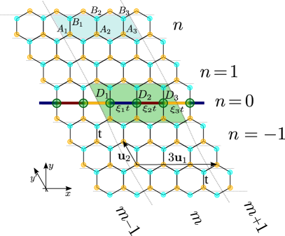
Figure 1: Scheme of a 3-periodic pentagon-only grain boundary. Notice that its unit cell has a periodicity of $3\mathbf{u}_{1}$ along the $x$-direction. The lattice vectors used are $3\mathbf{u}_{1}=3a(1,0)$ and $\mathbf{u}_{2}=(-1,\sqrt{3})a/2$. The hopping parameters at the defect alternate in value reading (in units of $t$): $\xi_{1}$, $\xi_{2}$ and $\xi_{3}$.

As is well known, graphene’s low energy charge carriers behave as massless Dirac fermions. These are governed by a Hamiltonian composed of two copies of the 2D Dirac Hamiltonian, each one of them valid around one of the two Dirac points.Semenoff (1984) In this limit the grain boundary essentially acts as a one-dimensional line that imposes a boundary condition on the Dirac spinors living on the semi-planes above and bellow the grain boundary. Such boundary condition will result in a discontinuity in the spinors across the defect and will control its scattering properties.Jiang et al. (2012); Rodrigues et al. (2012) In alternative, the grain boundary can also be thought of as a finite width strip containing a generalized potential that constrains the dynamics of the massless Dirac fermions.Rodrigues et al. (2012, 2013); Ebert et al. (2014)

The specific form of the boundary condition seen by the massless Dirac fermions at the 3-periodic pentagon-only grain boundary is determined by the details of its microscopic tight-binding model. In calculating it, we will follow the methodology developed for the cases of the pentagon-only, $zz(558)$ and $zz(5757)$ grain boundaries.Rodrigues et al. (2012, 2013) Below, we show that the boundary condition obtained from the tight-binding gives rise, in the low-energy limit, to a boundary condition explicitly introducing intervalley scattering. Furthermore, we will show how, starting from the grain boundary’s microscopic details, can we determine the generalized potential associated with viewing the grain boundary as a finite width strip with a potential constraining the Dirac fermions’ dynamics.

Before proceeding, we detail the structure of this text. In Section II we discuss general properties of Dirac fermion scattering off 3-periodic grain boundaries. In Section III we solve the electronic scattering off a 3-periodic pentagon-only grain boundary: we start by computing the tight-binding boundary condition matrix relating electronic amplitudes on each side of the grain boundary (see sub-Section III.1); we then derive the boundary condition matrix seen by the low-energy charge carriers (i.e. by the massless Dirac fermions) at the grain boundary (see sub-Section III.2); finally, in sub-Section III.3 we compute the transmission probabilities for different choices of the microscopic hopping parameters at the grain boundary. We close with Section IV where we overview the main results of the manuscript.

II General properties of low-energy electron transport across a 3-periodic grain boundary

Let us start by considering the case of a general 3-periodic grain boundary, i.e. a grain boundary with a periodicity (and orientation) defined by the vector $\mathbf{R}=n\mathbf{u}_{1}+m\mathbf{u}_{2}$, where $n,m\in\mathbb{N}$ and $n+m$ is a multiple of $3$ – see Fig. 1 where $n=3$ and $m=0$. The presence of such a grain boundary in graphene, breaks the translation symmetry along the direction perpendicular to the grain boundary. Furthermore, the periodicity of these grain boundaries happens to fold the first Brillouin zone in such a way that the two Dirac points are mapped into the $\Gamma$-point of the projected Brillouin zone. It is thus natural to expect that intervalley scattering off these nanostructures is generally allowed at low energies.

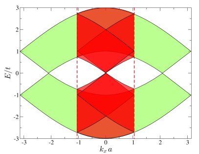
Figure 2: Pristine (and infinite) graphene energy spectrum projected along the $k_{y}$ direction (perpendicular to the defect). In green, the spectrum of pristine graphene (with the lattice vector along the zigzag direction given by $\mathbf{u}_{1}$). Its Dirac points are located at $k_{x}a=\pm 2\pi/3$. In red, the folded spectrum arising from choosing the lattice vector along the zigzag direction to be $3\mathbf{u}_{1}$. In this case, we can clearly see that the two Dirac points are mapped into $k_{x}a=0$.

As a consequence, when addressing the problem of electronic scattering across such kind of grain boundaries, we need to consider both valleys. Instead of working with two separate copies of the Dirac Hamiltonian $H_{\nu}=v_{F}\big{(}\nu\sigma_{1}\,\partial_{x}+\sigma_{2}\,\partial_{y}\big{)}$ valid in the vicinity of each Dirac point $\mathbf{K}_{\nu=\pm}$, we have to work with both copies simultaneously, i.e. with the Hamiltonian

$$H = v_{F}\big{(}\tau_{3}\otimes\sigma_{1}\,\partial_{x}+\tau_{0}\otimes\sigma_{2}\,\partial_{y}\big{)}\,,$$ (1)

where $\tau_{i}$ and $\sigma_{i}$ ($i=1,2,3$) stand for the $2\times 2$ Pauli matrices acting, respectively, on the valley and pseudo-spin degrees of freedom, while $\tau_{0}$ and $\sigma_{0}$ stand for the $2\times 2$ identity matrix. In the above equation (and in the remaining of this text) we have set $\hbar=1$. As we are considering a Hamiltonian that is independent of (real) spin, we will always omit the spin degree of freedom.

The presence of a periodic grain boundary in a graphene flake imposes a discontinuity between the Dirac fermion’s spinors on each of the grain boundary’s sides.Jiang et al. (2012); Rodrigues et al. (2012, 2013); Ebert et al. (2014) However, grain boundaries that are $3$-periodic also connect the two valleys through non-zero intervalley scattering matrix elements. For simplicity, let us consider the case of a zigzag-aligned (i.e. $x$-aligned) $3$-periodic grain boundary located at $y=0$. Such a grain boundary imposes the following general boundary condition on the Dirac spinors:

$$\Psi(x,0^{+}) = \mathcal{M}\Psi(x,0^{-})\,,$$ (2)

where $\Psi(\mathbf{r})=[\psi_{+}(\mathbf{r}),\psi_{-}(\mathbf{r})]^{T}$ are $4$-spinors since $\psi_{\pm}=[\varphi_{a\pm}(\mathbf{r}),\varphi_{b\pm}(\mathbf{r})]^{T}$ stands for the 2-spinor describing Dirac fermions living in the $\mathbf{K}_{\pm}$ valley. The $4\times 4$ matrix $\mathcal{M}$ can be written in the general form

$$\mathcal{M} = \left[\begin{array}[]{cc}\mathcal{M}_{++}&\mathcal{M}_{+-}\\ \mathcal{M}_{-+}&\mathcal{M}_{--}\end{array}\right]\,,$$ (5)

where $\mathcal{M}_{\pm\pm}$ ($\mathcal{M}_{\pm\mp}$) are $2\times 2$ matrices controlling the valley preserving (intervalley) scattering across the grain boundary.

The matrix $\mathcal{M}$ must satisfy the flux conservation condition $\mathcal{M}^{\dagger}J_{y}\mathcal{M}=J_{y}$, where $J_{y}=\tau_{0}\otimes\sigma_{y}$ stands for the conserved current along the direction perpendicular to the grain boundary. This stems from the hermiticity of the tight-binding Hamiltonian (that enforces current conservation at the GB in the tight-binding model). Furthermore, whenever we deal with non-magnetic grain boundaries, the boundary condition must as well be time-reversal invariant $\mathcal{T}^{-1}\mathcal{M}\mathcal{T}=\mathcal{M}$. Recall that the time-reversal operation exchanges the two Dirac cones and applies complex conjugation, $\mathcal{T}=\tau_{1}\otimes\sigma_{0}\,\mathcal{C}$.

A Dirac fermion from the $\mathbf{K}_{\nu}$ valley ($\nu=\pm 1$), incoming from $y=-\infty$ (see Fig. 1) will be partially transmitted and partially reflected at the grain boundary. In the absence of a potential difference between the two sides of the grain boundary, the wave function reads

$$\Psi^{L}(\mathbf{r}) = \Psi_{\mathbf{q},s}^{\nu,>}(\mathbf{r})+\rho_{\nu,\nu}\,\Psi_{\mathbf{q},s}^{\nu,<}(\mathbf{r})+\rho_{-\nu,\nu}\,\Psi_{\mathbf{q},s}^{-\nu,<}(\mathbf{r})\,,$$ (6a)

on the lower half-plane (i.e. $$y<0 y>0$$), while for the upper half-plane (i.e. ) we have

$$\Psi^{U}(\mathbf{r}) = \tau_{\nu,\nu}\,\Psi_{\mathbf{q},s}^{\nu,>}(\mathbf{r})+\tau_{-\nu,\nu}\,\Psi_{\mathbf{q},s}^{-\nu,>}(\mathbf{r})\,.$$ (6b)

In Eqs. (6) the $\Psi_{\mathbf{q},s}^{\nu,\lessgtr}(\mathbf{r})$ are 4-spinors which read

$$\Psi_{\mathbf{q}s}^{+,>}(\mathbf{r}) = \frac{1}{\sqrt{2}}\left[\begin{array}[]{cccc}s\,e^{-i\theta_{\mathbf{q}}^{+}},&1,&0,&0\end{array}\right]^{T}e^{i(q_{x}x+q_{y}y)}\,,$$ (7b)

$$\Psi_{\mathbf{q}s}^{-,>}(\mathbf{r}) = \frac{1}{\sqrt{2}}\left[\begin{array}[]{cccc}0,&0,&s\,e^{-i\theta_{\mathbf{q}}^{-}},&1\end{array}\right]^{T}e^{i(q_{x}x+q_{y}y)}\,,$$ (7d)

$$\Psi_{\mathbf{q}s}^{+,<}(\mathbf{r}) = \frac{1}{\sqrt{2}}\left[\begin{array}[]{cccc}s\,e^{-i\bar{\theta}_{\mathbf{q}}^{+}},&1,&0,&0\end{array}\right]^{T}e^{i(q_{x}x-q_{y}y)}\,,$$ (7f)

$$\Psi_{\mathbf{q}s}^{-,<}(\mathbf{r}) = \frac{1}{\sqrt{2}}\left[\begin{array}[]{cccc}0,&0,&s\,e^{-i\bar{\theta}_{\mathbf{q}}^{-}},&1\end{array}\right]^{T}e^{i(q_{x}x-q_{y}y)}\,.$$ (7h)

In the above expressions $\mathbf{r}=(x,y)$, $\mathbf{q}=(q_{x},q_{y})$, while $\theta_{\mathbf{q}}^{\nu}$ and $\bar{\theta}_{\mathbf{q}}^{\nu}=-\theta_{\mathbf{q}}^{\nu}$ stand for the complex phases of, respectively, $\nu q_{x}+iq_{y}$ and $\nu q_{x}-iq_{y}$. Furthermore, $s$ stands for the sign of the energy, distinguishing electrons and and holes, while $\rho_{\pm,\pm}$ ($\rho_{\pm,\mp}$) and $\tau_{\pm,\pm}$ ($\tau_{\pm,\mp}$) respectively stand for the valley preserving (intervalley) reflection and transmission coefficients.

Since the conserved current associated with a given propagating mode is the same for all modes, then the four transmission and reflection probabilities are simply given by $T_{\nu\eta}=|\tau_{\nu\eta}|^{2}$ and $R_{\nu\eta}=|\rho_{\nu\eta}|^{2}$, for $\nu=\pm 1$ and $\eta=\pm 1$. The transmission and reflection coefficients are obtained by solving the system of linear equations originating from imposing the boundary condition Eq. (2) on the wave function written in Eqs. (6) and (7). Therefore, the transmission and reflection probabilities will not only depend on the angle of incidence of the electron into the GB, but will also (strongly) depend on the microscopic properties of the grain boundary through the matrix elements of $\mathcal{M}$. Below, following Refs. Rodrigues et al., 2012, 2013, we will show how can we compute the boundary condition matrix $\mathcal{M}$ from the tight-binding model of the grain boundary.

However, before proceeding we will briefly discuss an often useful alternative viewpoint for such scattering problems (see Ref. Rodrigues et al., 2012, 2013). Instead of considering that in the low-energy limit the grain boundary simply imposes a discontinuity on the massless Dirac fermions’ spinors along a line parallel to the $x$-axis, we will consider that the grain boundary can be viewed as a finite strip of width $W$ that exists in $|y|<W/2$ and extends along the $x$ direction – see right-hand-side of Fig. 3. On each side of this strip the Dirac fermions will be governed by Eq. (1), while inside the strip there will also be a general local potential of the form

$$\mathbb{V} = \sum_{\alpha,\beta=0}^{3}V_{\alpha\beta}\,\tau_{\alpha}\otimes\sigma_{\beta}\,.$$ (8)

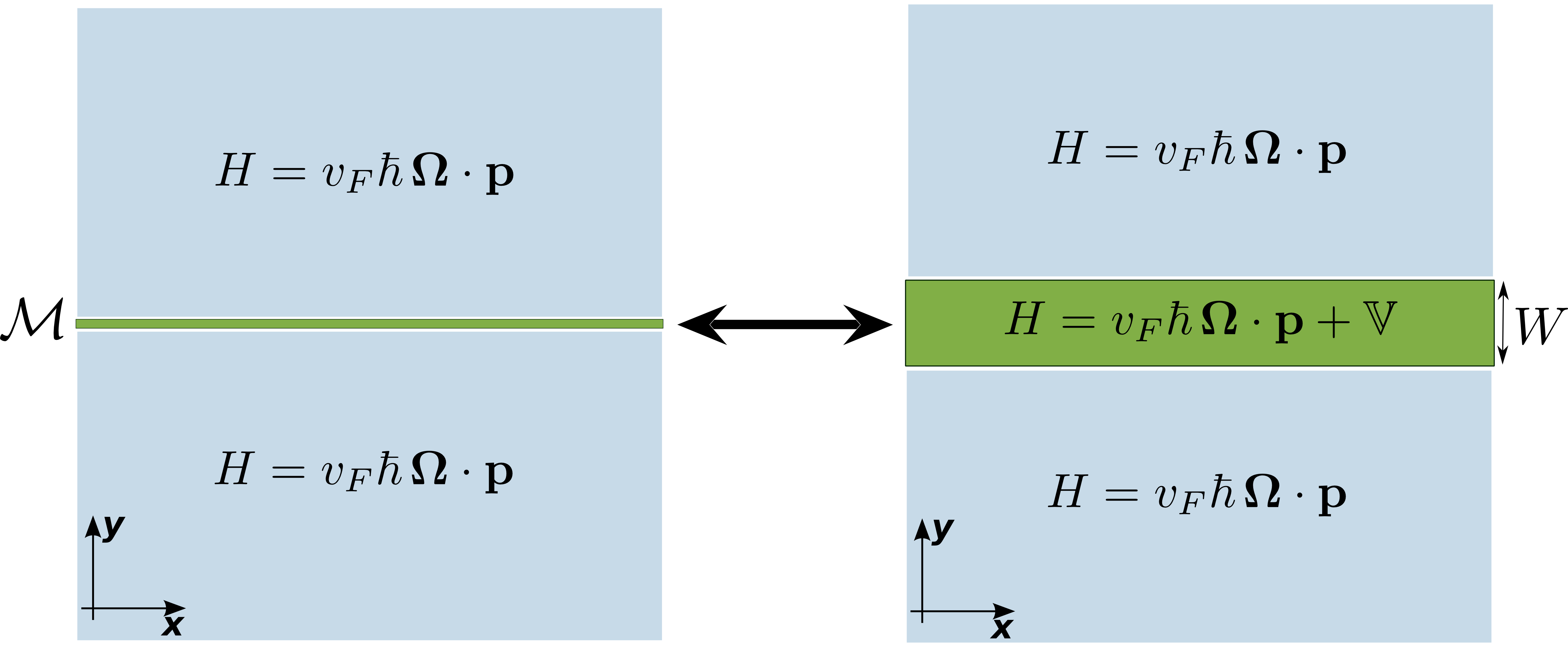
Figure 3: Schematic representation of the two perspectives used to analyze how do graphene’s low-energy charge carriers scatter off a grain boundary. On the left-hand-side, the massless Dirac fermions are constrained by $\Psi(x,0^{+})=\mathcal{M}\Psi(x,0^{-})$, which gives rise to a discontinuity of the Dirac spinors at the line separating the two half-planes [where the Dirac Hamiltonian governs the physics: $H=v_{F}\,\bm{\Omega}\cdot\mathbf{p}$, with $\bm{\Omega}\equiv(\tau_{3}\otimes\sigma_{1},\tau_{0}\otimes\sigma_{2})$]. On the right-hand-side, these two half-planes are separated by a finite width strip where the Dirac fermions are subject to a generalized potential $\mathbb{V}$.

The equivalence between these two viewpoints becomes obvious when we integrate out the Dirac equation in the finite width strip (i.e. between $-W/2<y<W/2$) while satisfying the constrain $W\times V_{\alpha\beta}\to v_{\alpha\beta}$ as $W\to 0$. As we show in detail in Appendix C, this integration gives rise to the following boundary condition matrix

$$\mathcal{M} = e^{{-i\frac{\tau_{0}\otimes\sigma_{2}}{v_{F}}\mathbb{V}}}\,,$$ (9)

which allows us to connect the matrix elements of $\mathcal{M}$ (determined from a tight-binding microscopic model) and the effective generalized local potential felt by the Dirac fermions inside the finite width strip.

Within this perspective, there are two interfaces at which we must ensure the continuity of the wave function, namely $\Psi(x,-w^{-})=\Psi(x,-w^{+})$ and $\Psi(x,w^{-})=\Psi(x,w^{+})$ where $w=W/2$. These two equalities correspond to eight conditions ($\Psi$ are 4-spinors) that will determine the eight unknown scattering coefficients (region inside the strip requires four additional coefficients).

III The 3-periodic pentagon-only grain boundary

In what follows we will make the statements of the previous section concrete by investigating the electronic transport across the 3-periodic pentagon-only grain boundary (see Fig. 1). We will start by briefly sketching how can we compute the tight-binding boundary condition matrix relating the wave function above and below the grain boundaryRodrigues et al. (2013); Páez et al. (2015) – see sub-Section III.1. From that result we will then compute the boundary condition matrix seen by the massless Dirac fermions at the grain boundary – see sub-Section III.2. Finally, in sub-Section III.3 we will work out the scattering problem and analyze the valley preserving and intervalley transmittance for specific sets of microscopic parameters defining the 3-periodic pentagon-only grain boundary.

III.1 The tight-binding model for the grain boundary

Consider a first-neighbor tight-binding model for electrons in the $p_{\textrm{z}}$-orbitals of graphene, where we define the pristine honeycomb direct lattice vectors as (see Fig. 1): $\mathbf{u}_{1}=a(1,0)$ and $\mathbf{u}_{2}=(-1,\sqrt{3})a/2$. As we want to study a zigzag-oriented grain boundary with periodicity $3\mathbf{u}_{1}$, we choose a bulk unit cell defined by the lattice vectors $3\mathbf{u}_{1}$ and $\mathbf{u}_{2}$ as sketched in Fig. 1. Fourier transforming along the $3\mathbf{u}_{1}$ direction diagonalizes the system’s Hamiltonian with respect to the variable $m$, introducing the quantum number $k_{x}$. The corresponding bulk tight-binding equations can then be written as

$$-\frac{\epsilon}{t}\mathbf{A}(n) = W_{A}^{\dagger}\mathbf{B}(n-1)+\mathbf{B}(n)\,,$$ (10a)

$$-\frac{\epsilon}{t}\mathbf{B}(n) = \mathbf{A}(n)+W_{A}\mathbf{A}(n+1)\,,$$ (10b)

where $\mathbf{Z}(n)=[Z_{1}(n),Z_{2}(n),Z_{3}(n)]^{T}$ for $Z=A,B$ and the matrix $W_{A}$ is defined in Eq. (36).

Eqs. (10) can be condensed in the form of a transfer matrix equationRodrigues et al. (2012, 2013) relating amplitudes at the atoms of the unit cell located at $\mathbf{r}=(n-1)\mathbf{u}_{2}$ with the amplitudes at the atoms of the unit cell located at $\mathbf{r}=n\mathbf{u}_{2}$. Such an equation reads

$$\mathbf{L}(n) = \mathbb{T}(\epsilon,k_{x})\mathbf{L}(n-1)\,,$$ (11)

with $\mathbf{L}(n)=[A_{1}(n),B_{1}(n),A_{2}(n),B_{2}(n),A_{3}(n),B_{3}(n)]^{T}$, while the transfer matrix $\mathbb{T}(\epsilon,k_{x})$ is given by

$$\mathbb{T}(\epsilon,k_{x}) = R\,\mathbb{Q}_{1}\,\mathbb{Q}_{2}\,R^{T}\,.$$ (12)

In the above equation, matrix $R$ is simply used to change from the basis $\{B_{1},B_{2},B_{3},A_{1},A_{2},A_{3}\}$ into the basis $\{A_{1},B_{1},A_{2},B_{2},A_{3},B_{3}\}$. This matrix is written in Eq. (45), while matrices $\mathbb{Q}_{1}$ and $\mathbb{Q}_{2}$ are written in Eqs. (38).

As was shown in Ref. Páez et al., 2015, we can employ a basis transformation $\widetilde{\mathbf{L}}(n)=\Lambda(k_{x})\mathbf{L}(n)$ that makes the transfer matrix block diagonal, $\widetilde{\mathbb{T}}=\textrm{diag}[\mathbb{T}_{h},\mathbb{T}_{l-},\mathbb{T}_{l+}]$. We will use the notation $\widetilde{\mathbf{L}}(n)=\{A_{h},B_{h},A_{l-},B_{l-},A_{l+},B_{l+}\}$ to identify the elements of a vector in this basis. The three matrices $\mathbb{T}_{h}$, $\mathbb{T}_{l-}$ and $\mathbb{T}_{l+}$ on the diagonal of $\widetilde{\mathbb{T}}$ are $2\times 2$ matrices that depend on both $\epsilon$ and $k_{x}a$. They are written in Eq. (53), while the matrix $\Lambda(k_{x})$ is written in Eq. (52). Each one of the $\mathbb{T}_{h}$, $\mathbb{T}_{l-}$ and $\mathbb{T}_{l+}$ matrices correspond to one of the three propagation modes of the problem. Around $k_{x}a=0$ two of these modes are low-energy (corresponding to each of the two Dirac cones), while the other one is a high-energy mode – see Appendix A.1.

In a similar way, we can compute the boundary condition matrix that relates electronic amplitudes below and above the 3-periodic pentagon-only grain boundary (see Fig. 1). We start by writing the tight-binding equations in the grain boundary regionRodrigues et al. (2012, 2013); Páez et al. (2015) (we neglect out-of-plane relaxations in the GB region)

$$-\frac{\epsilon}{t}\mathbf{A}(1) = W_{A}^{\dagger}\mathbf{B}(0)+\mathbf{B}(1)\,,$$ (13a)

$$-\frac{\epsilon}{t}\mathbf{B}(0) = \mathbf{D}(0)+W_{A}\mathbf{A}(1)\,,$$ (13b)

$$-\frac{\epsilon}{t}\mathbf{D}(0) = \mathbf{B}(0)+\sigma_{x}^{\prime}\mathbf{D}(0)+\mathbf{A}(0),$$ (13c)

$$-\frac{\epsilon}{t}\mathbf{A}(0) = \mathbf{D}(0)+W_{A}^{\dagger}\mathbf{B}(-1)\,,$$ (13d)

$$-\frac{\epsilon}{t}\mathbf{B}(-1) = \mathbf{A}(-1)+W_{A}\mathbf{A}(0)\,,$$ (13e)

where the matrix $\sigma_{x}^{\prime}$ is written in Eq. (58). Note that $\sigma_{x}^{\prime}$ depends both on $k_{x}a$ and on the hopping parameters at the grain boundary, $\xi_{1}$, $\xi_{2}$ and $\xi_{3}$.

We can express these equations (see Appendix A.2) as a boundary condition equation connecting the electronic wave function on the two sides of the grain boundary

$$\mathbf{L}(1) = \mathbb{M}\,\mathbf{L}(-1)\,.$$ (14)

The boundary condition matrix $\mathbb{M}$ above is a $6\times 6$ matrix given by

$$\mathbb{M} = R\mathbb{N}_{1}\mathbb{N}_{2}\mathbb{N}_{3}\mathbb{N}_{1}\mathbb{N}_{2}R^{T}\,,$$ (15)

where, for the sake of simplicity, we have omitted the dependence of the matrices $\mathbb{M}$ and $\mathbb{N}_{i}$ on $\epsilon/t$, $k_{x}$ and $\xi_{i}$. The matrices $\mathbb{N}_{i}$ are written in Eqs. (60).

Finally, we can write the boundary condition matrix $\mathbb{M}$ in the basis uncoupling the three pairs of modes of the transfer matrix, $\widetilde{\mathbb{M}}=\Lambda(k_{x}a)\mathbb{M}[\Lambda(k_{x}a)]^{-1}$. By inspecting the boundary condition Eq. (14) in this basis, $\widetilde{\mathbf{L}}(1)=\widetilde{\mathbb{M}}\,\widetilde{\mathbf{L}}(-1)$, we readily conclude that, in general, $\widetilde{\mathbb{M}}$ mixes all the three modes of the transfer matrix (both the high-energy and the two low-energy ones).

III.2 The boundary condition in the low-energy approximation

At very low energies, $\epsilon\to 0$, and very near the Dirac points, $\mathbf{k}\to\mathbf{K}_{\nu}=(0,-1)\nu 4\pi/(3\sqrt{3}a)$, the matrix $\widetilde{\mathbb{M}}$ acquires a somewhat simple form – see Eq. (LABEL:eq:MatDiracPnt). In this limit, the high-energy modes are evanescent, one of them increasing and the other one decreasing exponentially with $n$ – see Eq. (LABEL:eq:TMdiags1-LowE-limit) and subsequent paragraph. Since we must require the wave function to be normalizable, we conclude that when $\epsilon\to 0$ and $\mathbf{k}\to\mathbf{K}_{\nu}$ the wave function must have the following form

$$\widetilde{\mathbf{L}}(n) \approx \widetilde{\mathbf{l}}(n)=\left[\begin{array}[]{c}A_{h}(n)\\ 0\\ A_{l-}(n)\\ B_{l-}(n)\\ A_{l+}(n)\\ B_{l+}(n)\end{array}\right],\,\,\textrm{for $n>0$,}$$ (16g)

and

$$\widetilde{\mathbf{L}}(n) \approx \widetilde{\mathbf{l}}(n)=\left[\begin{array}[]{c}0\\ B_{h}(n)\\ A_{l-}(n)\\ B_{l-}(n)\\ A_{l+}(n)\\ B_{l+}(n)\end{array}\right],\,\,\textrm{for $n<0$,}$$ (16n)

where, in order to keep the notation lighter, we have omitted the dependence on $k_{x}$ of both the vectors $\widetilde{\mathbf{L}}$ and $\widetilde{\mathbf{l}}$, and of the amplitudes $A$ and $B$.

We can now substitute Eqs. (16) in the boundary condition $\widetilde{\mathbf{L}}(1)=\widetilde{\mathbb{M}}\,\widetilde{\mathbf{L}}(-1)$ to eliminate the high energy modes from our problem, ending up with an effective boundary condition that only involves the low-energy modes. Such a manipulation generates an effective boundary condition matrix $\mathbb{M}^{\textrm{eff}}$ that we can express in terms of the matrix elements of $\widetilde{\mathbb{M}}$ as follows

$$\mathbb{M}^{\textrm{eff}} = \left[\begin{array}[]{cccc}\widetilde{\mathbb{M}}_{33}-\frac{\widetilde{\mathbb{M}}_{32}\widetilde{\mathbb{M}}_{23}}{\widetilde{\mathbb{M}}_{22}}&\widetilde{\mathbb{M}}_{34}-\frac{\widetilde{\mathbb{M}}_{32}\widetilde{\mathbb{M}}_{24}}{\widetilde{\mathbb{M}}_{22}}&\widetilde{\mathbb{M}}_{35}-\frac{\widetilde{\mathbb{M}}_{32}\widetilde{\mathbb{M}}_{25}}{\widetilde{\mathbb{M}}_{22}}&\widetilde{\mathbb{M}}_{36}-\frac{\widetilde{\mathbb{M}}_{32}\widetilde{\mathbb{M}}_{26}}{\widetilde{\mathbb{M}}_{22}}\\ \widetilde{\mathbb{M}}_{43}-\frac{\widetilde{\mathbb{M}}_{42}\widetilde{\mathbb{M}}_{23}}{\widetilde{\mathbb{M}}_{22}}&\widetilde{\mathbb{M}}_{44}-\frac{\widetilde{\mathbb{M}}_{42}\widetilde{\mathbb{M}}_{24}}{\widetilde{\mathbb{M}}_{22}}&\widetilde{\mathbb{M}}_{45}-\frac{\widetilde{\mathbb{M}}_{42}\widetilde{\mathbb{M}}_{25}}{\widetilde{\mathbb{M}}_{22}}&\widetilde{\mathbb{M}}_{46}-\frac{\widetilde{\mathbb{M}}_{42}\widetilde{\mathbb{M}}_{26}}{\widetilde{\mathbb{M}}_{22}}\\ \widetilde{\mathbb{M}}_{53}-\frac{\widetilde{\mathbb{M}}_{52}\widetilde{\mathbb{M}}_{23}}{\widetilde{\mathbb{M}}_{22}}&\widetilde{\mathbb{M}}_{54}-\frac{\widetilde{\mathbb{M}}_{52}\widetilde{\mathbb{M}}_{24}}{\widetilde{\mathbb{M}}_{22}}&\widetilde{\mathbb{M}}_{55}-\frac{\widetilde{\mathbb{M}}_{52}\widetilde{\mathbb{M}}_{25}}{\widetilde{\mathbb{M}}_{22}}&\widetilde{\mathbb{M}}_{56}-\frac{\widetilde{\mathbb{M}}_{52}\widetilde{\mathbb{M}}_{26}}{\widetilde{\mathbb{M}}_{22}}\\ \widetilde{\mathbb{M}}_{63}-\frac{\widetilde{\mathbb{M}}_{62}\widetilde{\mathbb{M}}_{23}}{\widetilde{\mathbb{M}}_{22}}&\widetilde{\mathbb{M}}_{64}-\frac{\widetilde{\mathbb{M}}_{62}\widetilde{\mathbb{M}}_{24}}{\widetilde{\mathbb{M}}_{22}}&\widetilde{\mathbb{M}}_{65}-\frac{\widetilde{\mathbb{M}}_{62}\widetilde{\mathbb{M}}_{25}}{\widetilde{\mathbb{M}}_{22}}&\widetilde{\mathbb{M}}_{66}-\frac{\widetilde{\mathbb{M}}_{62}\widetilde{\mathbb{M}}_{26}}{\widetilde{\mathbb{M}}_{22}}\end{array}\right]\,.$$ (21)

The matrix $\mathbb{M}^{\textrm{eff}}$ for the case of the 3-periodic pentagon-only grain boundary is written in Eqs. (77) and (78).

As is widely known, in the low-energy continuum limit the tight-binding amplitudes, $C(\mathbf{r})$, can be expressed in terms of slowly varying fields, $\psi_{c}(\mathbf{r})$, as

$$C(\mathbf{r}) \approx \sum_{\nu=\pm 1}e^{i\mathbf{K}_{\nu}\cdot\mathbf{r}}\psi_{c}^{\nu}(\mathbf{r})\,.$$ (22)

We can thus cast the tight-binding 4-spinor valid at low-energies, $\bm{\ell}(\mathbf{r})=[A_{l-}(\mathbf{r}),B_{l-}(\mathbf{r}),A_{l+}(\mathbf{r}),B_{l+}(\mathbf{r})]^{T}$, in terms of slowly varying Dirac fields as $\bm{\ell}(\mathbf{r})\approx[e^{i\mathbf{K}_{-}\cdot\mathbf{r}}\psi_{-}(\mathbf{r}),e^{i\mathbf{K}_{+}\cdot\mathbf{r}}\psi_{+}(\mathbf{r})]^{T}$, where $\psi_{\nu}(\mathbf{r})=[\psi_{a_{\nu}},\psi_{b_{\nu}}]^{T}$.

We can finally write the boundary condition that Dirac fermions see at the 3-periodic pentagon-only grain boundary as $\Psi(x,0^{+})=\mathcal{M}\Psi(x,0^{-})$, where $\Psi(\mathbf{r})=[\Psi_{-}(\mathbf{r}),\Psi_{+}(\mathbf{r})]^{T}=[\psi_{a_{-}}(\mathbf{r}),\psi_{b_{-}}(\mathbf{r}),\psi_{a_{+}}(\mathbf{r}),\psi_{b_{+}}(\mathbf{r})]^{T}$.

In the case of the 3-periodic pentagon-only grain boundary, the matrix $\mathcal{M}$ (see Appendix B) reads

$$\mathcal{M} = \left[\begin{array}[]{cccc}0&1&0&0\\ -1&f&0&g^{*}\,e^{i\frac{2\pi}{3}}\\ 0&0&0&1\\ 0&g\,e^{-i\frac{2\pi}{3}}&-1&f\end{array}\right]\,,$$ (27)

where $f\equiv f(\xi_{1},\xi_{2},\xi_{3})$ and $g\equiv g(\xi_{1},\xi_{2},\xi_{3})$ are written in Eqs. (78).

Interestingly, in Eq. (27) we clearly see that the off-diagonal blocks of matrix $\mathcal{M}$, those which control the intervalley scattering, are not a priori zero. We can thus conclude that in general this grain boundary gives rise to intervalley scattering. In particular, the intervalley scattering mixes the $\psi_{b}$ component of one valley with the same component of the other valley.

Notice that when all the three hoppings are equal (i.e. $\xi_{1}=\xi_{2}=\xi_{3}=\xi$), we get back to the simple case of the pentagon-only grain boundary (with periodicity $p=1$) that, as we know,Rodrigues et al. (2012) does not give rise to intervalley scattering. Owing to the fact that $f(\xi,\xi,\xi)=\xi$ and $g(\xi,\xi,\xi)=0$ [see Eqs. (78)], its boundary condition matrix reads

$$\mathcal{M} = \left[\begin{array}[]{cccc}0&1&0&0\\ -1&\xi&0&0\\ 0&0&0&1\\ 0&0&-1&\xi\end{array}\right]\,.$$ (32)

But this is natural since in such a case we are effectively dealing with a grain boundary with periodicity $\mathbf{u}_{1}$ which maps the projected Dirac points into distinct values of $k_{x}$ – see Fig. 2. Similarly, when we set $\xi_{1}=\xi_{2}=\xi$ and $\xi_{3}=0$, we recover the case of the $zz(558)$ grain boundary, which owing to its periodicity of $2\mathbf{u}_{1}$ also maps the projected Dirac points into distinct values of $k_{x}$, which ends up blocking intervalley scattering.Gunlycke and White (2011); Jiang et al. (2011, 2012); Rodrigues et al. (2012, 2013); Ebert et al. (2014); Páez et al. (2015)

Moreover, there are a few cases where, despite the 3-periodicity of the grain boundary, intervalley scattering is suppressed. In these cases, the microscopic details of the grain boundary, i.e. the precise values of $\xi_{1}$, $\xi_{2}$ and $\xi_{3}$, force $g(\xi_{1},\xi_{2},\xi_{3})=0$ thus forbidding intervalley scattering. Examples of such cases are: $\xi_{3}=-3\xi_{1}$ and $\xi_{2}=\xi_{1}$; $\xi_{3}=-\xi_{1}/3$ and $\xi_{2}=-\xi_{1}/3$; and $\xi_{3}=\xi_{1}$ and $\xi_{2}=-3\xi_{1}$.

In the context of the perspective where we consider the grain boundary to be a finite width strip with a generalized potential [see Eq. (8) and end of Section II], we show in Appendix C that the generalized potential originating from the 3-periodic pentagon-only grain boundary both has valley preserving terms (such as $V_{00}$ - a scalar potential - and $V_{01}$ - a constant gauge potential), and valley mixing terms (such as $V_{10}$, $V_{20}$, $V_{11}$ and $V_{21}$). As a consequence, in general, a 3-periodic pentagon-only grain boundary will not only generate intervalley scattering, but it will also prevent the existence of an angle of perfect transmission (see Appendix C).

III.3 The Transmittance

As discussed in Section II we can now compute the transmission and reflection coefficients $\tau_{\pm\pm}$, $\tau_{\pm\mp}$, $\rho_{\pm\pm}$ and $\rho_{\pm\mp}$. In particular, the transmission probability for an incoming electron living on the $\mathbf{K}_{+}$ ($\mathbf{K}_{-}$) valley to be transmitted into the same valley is given by $T_{++}=|\tau_{++}|^{2}$ ($T_{--}=|\tau_{--}|^{2}$), while the probability for it to be transmitted into the other valley is given by $T_{-+}=|\tau_{-+}|^{2}$ ($T_{+-}=|\tau_{+-}|^{2}$).

In Eqs. (80) we write the expressions of the $\tau_{++}$, $\tau_{-+}$, $\tau_{+-}$ and $\tau_{--}$, for the 3-periodic pentagon-only grain boundary with general hoppings (in units of $t$), $\xi_{1}$, $\xi_{2}$ and $\xi_{3}$. These were obtained by solving the system of linear equations defined by $\Psi(x,0^{+})=\mathcal{M}\Psi(x,0^{-})$ where $\mathcal{M}$ is given by Eq. (27). In Fig. 4 we have plotted the transmission probabilities $T_{\pm\pm}$ and $T_{\pm\mp}$ for the case where the hopping parameters are $\xi_{1}=0.1$, $\xi_{2}=0.4$ and $\xi_{3}=0.8$.

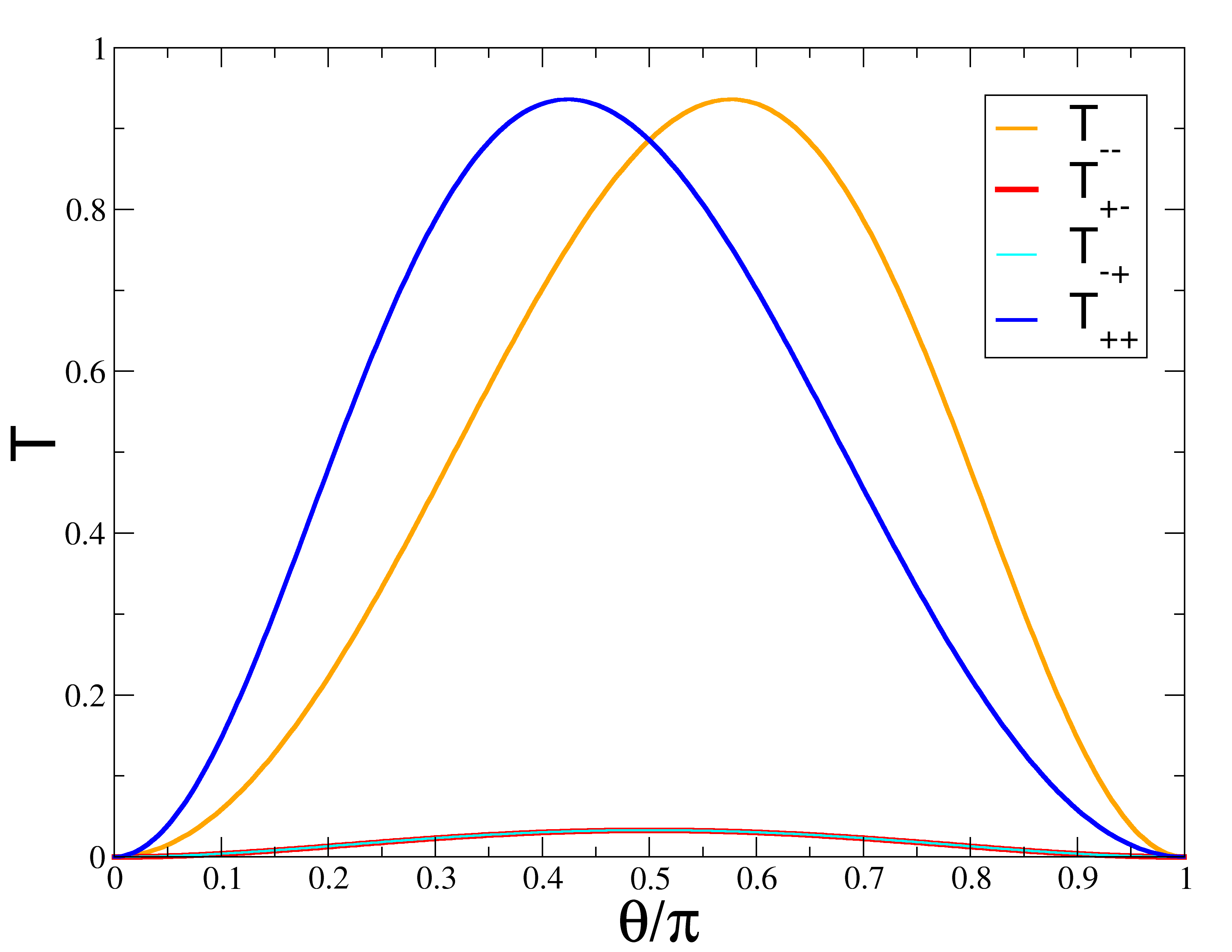
Figure 4: Massless Dirac fermions’ transmission probabilities for the 3-periodic pentagon-only grain boundary in terms of the angle of incidence, $\theta$. The $T_{--}$ ($T_{+-}$) [$T_{-+}$ ($T_{++}$)] stands for the probability of transmission of an incident Dirac fermion living on the $\mathbf{K}_{-}$ [$\mathbf{K}_{+}$] valley to be transmitted into the $\mathbf{K}_{-}$ ($\mathbf{K}_{+}$) valley. The hopping parameters at the grain boundary were set to: $\xi_{1}=0.1t$, $\xi_{2}=0.4t$ and $\xi_{3}=0.8t$.

For a 3-periodic pentagon-only grain boundary with the above hopping parameters, the intervalley scattering is weak, with the intervalley transmission probabilities being considerably smaller than the valley preserving ones. However, this picture can be greatly modified if we choose an appropriate set of hopping parameters at the grain boundary. As an example, in Fig. 5 we plot the transmission probabilities for a case where $\xi_{1}=1.1$, $\xi_{2}=0.05$ and $\xi_{3}=2.2$, which shows much stronger intervalley scattering than Fig. 4.

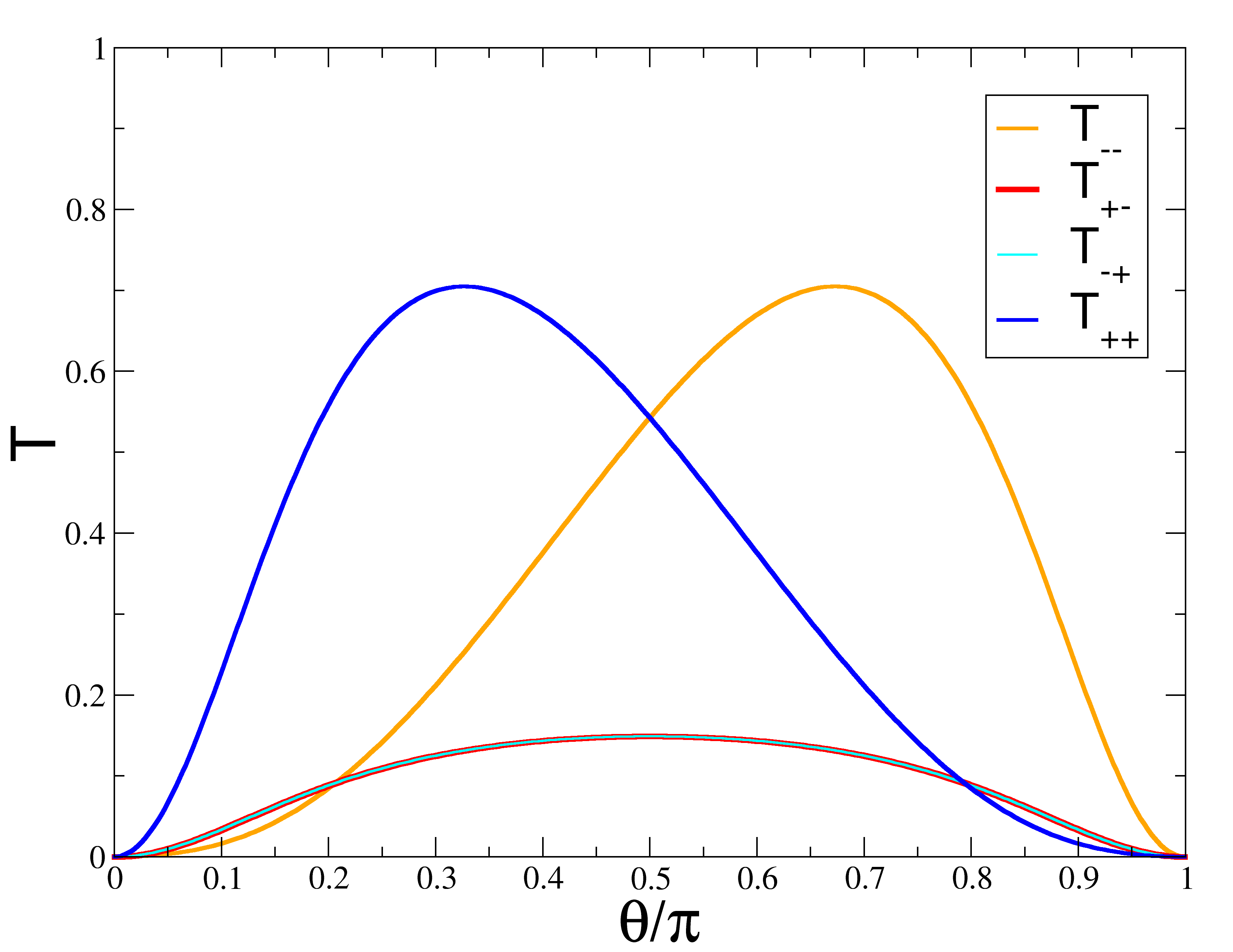
Figure 5: Same as in Fig. 4, but now with the hopping parameters at the grain boundary set to: $\xi_{1}=1.1t$, $\xi_{2}=0.05t$ and $\xi_{3}=2.2t$.

This robust increase of the intervalley transmission (compare Figs. 4 and 5) can be traced back to a strong amplification of the terms $V_{10}$ and $V_{11}$ of the generalized potential existent inside the strip that mimics the effect of the grain boundary in the low-energy limit. Such an amplification (by nearly two orders of magnitude) gives rise to a set of generalized potential terms of similar magnitudes, thus increasing the amount of valley mixing of the eigenmodes living inside the strip. The stronger the valley mixing of these modes, the more the electron’s valley quantum number rotates while propagating inside the strip, and thus more wave function weight is transferred between valleys while the Dirac fermion propagates inside the strip.

Finally, we must note that, as we can quickly infer from the above results (where we have considered different sets of values for the hopping renormalizations $\xi_{i}$), the scattering properties of the grain boundary are strongly dependent on the microscopic details at the grain boundary, as previously remarked by other studies.Rodrigues et al. (2012, 2013); Páez et al. (2015) Such behaviour points towards the possibility of making use of this kind of nanostructures to control and explore the valley degree of freedom of graphene. Chemical decoration of the grain boundary region, application of strains, of electric and of magnetic fields, all likely modify the electronic scattering off these grain boundaries, thus suggesting their usage as sensors and current switchers.

IV Conclusion

To close, let us briefly summarize the contents of this manuscript. We have started by analyzing in general terms the low-energy charge carrier transport across zigzag-aligned degenerate 3-periodic grain boundaries. We have then demonstrated such results by working out the low-energy charge transport across a 3-periodic pentagon-only grain boundary. In particular, starting from its microscopic tight-binding model, we have derived the boundary condition seen by the massless Dirac fermions at such grain boundary. With it we have calculated the scattering coefficients, from which we concluded that the valley preserving and intervalley scattering probabilities are highly responsive to external manipulation through control of the grain boundary’s microscopic details. We have also made use of the generalized potential representation of the grain boundary to gain insight into the obtained results.

Appendix A Tight-binding model

In this section we will give details of the derivations presented in Section III.1 concerning the microscopic tight-binding model of monolayer graphene with a 3-periodic pentagon-only grain boundary. The calculations below closely follow what was done in Ref. Páez et al., 2015. In sub-Section A.1 we concentrate on the calculations leading to the bulk transfer matrix, while in sub-Section A.2 we focus on the calculations giving rise to the tight-binding boundary condition that originates from the presence of the 3-periodic pentagon-only grain boundary.

A.1 The tight-binding equations at the bulk

The matrix $W_{A}$ present in the bulk tight-binding equations [see Eqs. (10)] reads

$$W_{A} = \left[\begin{array}[]{ccc}1&1&0\\ 0&1&1\\ e^{3ik_{x}a}&0&1\end{array}\right]\,.$$ (36)

The bulk tight-binding equations [see Eqs. (10)] can be cast in the form

$$\left[\begin{array}[]{c}\mathbf{B}(n)\\ \mathbf{A}(n)\end{array}\right] = \mathbb{Q}_{1}\left[\begin{array}[]{c}\mathbf{A}(n)\\ \mathbf{B}(n-1)\end{array}\right]\,,$$ (37e)

$$\left[\begin{array}[]{c}\mathbf{A}(n)\\ \mathbf{B}(n-1)\end{array}\right] = \mathbb{Q}_{2}\left[\begin{array}[]{c}\mathbf{B}(n-1)\\ \mathbf{A}(n-1)\end{array}\right]\,,$$ (37j)

where the matrices $\mathbb{Q}_{1}$ and $\mathbb{Q}_{2}$ read

$$\mathbb{Q}_{1} = -\left[\begin{array}[]{cc}\frac{\epsilon}{t}\mathbb{I}_{3}&W_{A}^{\dagger}\\ -\mathbb{I}_{3}&0\end{array}\right]\,,$$ (38c)

$$\mathbb{Q}_{2} = -\left[\begin{array}[]{cc}\frac{\epsilon}{t}\big{(}W_{A}\big{)}^{-1}&\big{(}W_{A}\big{)}^{-1}\\ -\mathbb{I}_{3}&0\end{array}\right]\,,$$ (38f)

with $\mathbb{I}_{3}$ standing for the $3\times 3$ unit matrix.

Eqs. (37) can be written in the form of a transfer matrix, as was done in Eq. (11), where the transfer matrix is given by Eq. (12). The matrix $R$ present in the latter equation reads

$$R = \left[\begin{array}[]{cccccc}0&0&0&1&0&0\\ 1&0&0&0&0&0\\ 0&0&0&0&1&0\\ 0&1&0&0&0&0\\ 0&0&0&0&0&1\\ 0&0&1&0&0&0\end{array}\right]\,.$$ (45)

This matrix simply changes from the basis $\{B_{1}(n),B_{2}(n),B_{3}(n),A_{1}(n),A_{2}(n),A_{3}(n)\}$ into the basis $\{A_{1}(n),B_{1}(n),A_{2}(n),B_{2}(n),A_{3}(n),B_{3}(n)\}$.

The matrix $\Lambda(\phi)$ enforcing the basis change that uncouples the modes of the transfer matrix reads

$$\Lambda(\phi) = \frac{1}{\sqrt{3}}\left[\begin{array}[]{cccccc}1&0&-\frac{e^{-i(\phi-2\pi/3)}i\sqrt{3}}{1+e^{i\pi/3}}&0&\frac{e^{-i2(\phi-2\pi/3)}i\sqrt{3}}{1+e^{-i\pi/3}}&0\\ 0&1&0&-\frac{e^{-i(\phi-2\pi/3)}i\sqrt{3}}{1+e^{i\pi/3}}&0&\frac{e^{-i2(\phi-2\pi/3)}i\sqrt{3}}{1+e^{-i\pi/3}}\\ 1&0&-e^{-i(\phi-\pi/3)}&0&-e^{-i(2\phi+\pi/3)}&0\\ 0&1&0&-e^{-i(\phi-\pi/3)}&0&-e^{-i(2\phi+\pi/3)}\\ 1&0&-e^{-i(\phi+\pi/3)}&0&-e^{-i(2\phi-\pi/3)}&0\\ 0&1&0&-e^{-i(\phi+\pi/3)}&0&-e^{-i(2\phi-\pi/3)}\end{array}\right]\,,$$ (52)

where $\phi=k_{x}a$.

In this basis, the three $2\times 2$ matrices in the diagonal of the transfer matrix $\widetilde{\mathbb{T}}(\epsilon,k_{x}a)$ are noted by $\mathbb{T}_{h}$, $\mathbb{T}_{l-}$ and $\mathbb{T}_{l+}$. The matrix

$$\mathbb{T}_{h}(\epsilon,k_{x}a) = \frac{1}{1+e^{ik_{x}a}}\left[\begin{array}[]{cc}-1&-\epsilon\\ \epsilon&-2-2\cos(k_{x}a)+\epsilon^{2}\end{array}\right]\,,$$ (53c)

corresponds to the high-energy mode when we are around $$k_{x}a=0$$. Similarly, the matrices corresponding to the low-energy modes (one from each Dirac point) read

$$\mathbb{T}_{l-}(\epsilon,k_{x}a) = \Upsilon(k_{x})\left[\begin{array}[]{cc}-1&-\epsilon\\ \epsilon&\frac{e^{-i(k_{x}a-\frac{\pi}{3})}-1}{f(k_{x})}+\epsilon^{2}\end{array}\right]\,,$$ (53g)

$$\mathbb{T}_{l+}(\epsilon,k_{x}a) = \Theta(k_{x})\left[\begin{array}[]{cc}-1&-\epsilon\\ \epsilon&\frac{e^{-i(k_{x}a+\frac{\pi}{3})}-1}{g(k_{x})}+\epsilon^{2}\end{array}\right]\,,$$ (53j)

where we have defined $\Upsilon(k_{x})$ and $\Theta(k_{x})$ as

$$\Upsilon(k_{x}) = \frac{e^{i\pi/3}-e^{-ik_{x}a}}{1-2\cos(k_{x}a)}\,,$$ (54a)

$$\Theta(k_{x}) = \frac{e^{-i\pi/3}-e^{-ik_{x}a}}{1-2\cos(k_{x}a)}\,.$$ (54b)

A.2 The tight-binding equations at the grain boundary

The matrix $\sigma_{x}^{\prime}$ present in the tight-binding equations at the grain boundary region [see Eqs. (13)] reads

$$\sigma_{x}^{\prime} = \left[\begin{array}[]{ccc}0&\xi_{1}&\xi_{3}e^{-3ik_{x}a}\\ \xi_{1}&0&\xi_{2}\\ \xi_{3}e^{3ik_{x}a}&\xi_{2}&0\end{array}\right]\,,$$ (58)

where $\xi_{1}$, $\xi_{2}$ and $\xi_{3}$ stand for the hopping parameters at the grain boundary region as represented in Fig. 1.

Eqs. (13) can be condensed in the form

$$\left[\begin{array}[]{c}\mathbf{B}(1)\\ \mathbf{A}(1)\end{array}\right] = \mathbb{N}_{1}\left[\begin{array}[]{c}\mathbf{A}(1)\\ \mathbf{B}(0)\end{array}\right]\,,$$ (59e)

$$\left[\begin{array}[]{c}\mathbf{A}(1)\\ \mathbf{B}(0)\end{array}\right] = \mathbb{N}_{2}\left[\begin{array}[]{c}\mathbf{B}(0)\\ \mathbf{D}(0)\end{array}\right],$$ (59j)

$$\left[\begin{array}[]{c}\mathbf{B}(0)\\ \mathbf{D}(0)\end{array}\right] = \mathbb{N}_{3}\left[\begin{array}[]{c}\mathbf{D}(0)\\ \mathbf{A}(0)\end{array}\right]\,,$$ (59o)

$$\left[\begin{array}[]{c}\mathbf{D}(0)\\ \mathbf{A}(0)\end{array}\right] = \mathbb{N}_{1}\left[\begin{array}[]{c}\mathbf{A}(0)\\ \mathbf{B}(-1)\end{array}\right]\,,$$ (59t)

$$\left[\begin{array}[]{c}\mathbf{A}(0)\\ \mathbf{B}(-1)\end{array}\right] = \mathbb{N}_{2}\left[\begin{array}[]{c}\mathbf{B}(-1)\\ \mathbf{A}(-1)\end{array}\right]\,.$$ (59y)

where the matrices $\mathbb{N}_{1}$, $\mathbb{N}_{2}$ and $\mathbb{N}_{3}$ are $6\times 6$ matrices which read

$$\mathbb{N}_{1} = -\left[\begin{array}[]{cc}\frac{\epsilon}{t}\mathbb{I}_{3}&\big{(}W_{A}\big{)}^{\dagger}\\ -\mathbb{I}_{3}&0\end{array}\right]\,,$$ (60c)

$$\mathbb{N}_{2} = -\left[\begin{array}[]{cc}\frac{\epsilon}{t}\big{(}W_{A}\big{)}^{-1}&\big{(}W_{A}\big{)}^{-1}\\ -\mathbb{I}_{3}&0\end{array}\right]\,,$$ (60f)

$$\mathbb{N}_{3} = -\left[\begin{array}[]{cc}\Big{(}\frac{\epsilon}{t}\mathbb{I}_{3}+\sigma_{x}^{\prime}\Big{)}&\mathbb{I}_{3}\\ -\mathbb{I}_{3}&0\end{array}\right]\,.$$ (60i)

The above matrices depend on the reduced energy, $\epsilon/t$, on the longitudinal momentum, $k_{x}$, and on the hopping parameters at the defect, $\xi_{1}$, $\xi_{2}$ and $\xi_{3}$.

Appendix B The boundary condition matrix in the continuum approximation

When $\epsilon\to 0$ and $\mathbf{k}\to\mathbf{K}_{\nu}=(0,-1)\nu 4\pi/(3\sqrt{3}a)$, the boundary condition matrix (expressed in the basis uncoupling the modes of the transfer matrix $\mathbb{T}$) $\widetilde{\mathbb{M}}$ reads

$$\widetilde{\mathbb{M}} = \left[\begin{array}[]{cccccc}0&1&0&0&0&0\\ -1&-\frac{8}{3}(\xi_{1}+\xi_{2}+\xi_{3})&0&\frac{2}{3}(-\xi_{1}+\xi_{2}e^{-i\pi/3}+\xi_{3}e^{i\pi/3})&0&\frac{2}{3}(-\xi_{1}+\xi_{2}e^{i\pi/3}+\xi_{3}e^{-i\pi/3})\\ 0&0&0&-e^{i\pi/3}&0&0\\ 0&\frac{2}{3}(\xi_{1}e^{i\pi/3}+\xi_{2}e^{-i\pi/3}-\xi_{3})&e^{i\pi/3}&-\frac{e^{i\pi/3}}{3}(\xi_{1}+\xi_{2}+\xi_{3})&0&\frac{2}{3}(\xi_{1}e^{i\pi/3}-\xi_{2}+\xi_{3}e^{-i\pi/3})\\ 0&0&0&0&0&-e^{-i\pi/3}\\ 0&\frac{2}{3}(\xi_{1}e^{-i\pi/3}+\xi_{2}e^{i\pi/3}-\xi_{3})&0&\frac{2}{3}(\xi_{1}e^{-i\pi/3}-\xi_{2}+\xi_{3}e^{i\pi/3})&e^{-i\pi/3}&-\frac{e^{-i\pi/3}}{3}(\xi_{1}+\xi_{2}+\xi_{3})\end{array}\right]\,.$$ (67)

In this limit, the $2\times 2$ matrix $\mathbb{T}_{h}$ describing the high energy modes of the transfer matrix $\widetilde{\mathbb{T}}$ [see Eq. (LABEL:eq:TMdiags1)] reads

$$\mathbb{T}_{h}(0,0) = -\left[\begin{array}[]{cc}\frac{1}{2}&0\\ 0&2\end{array}\right]\,.$$ (71)

It is then straightforward to understand what will be the relation between the high-energy modes’ amplitudes $\widetilde{\mathbf{L}}(i)$ at position $i$, and the amplitudes $\widetilde{\mathbf{L}}(j)=\widetilde{\mathbb{T}}^{n}\widetilde{\mathbf{L}}(i)$ at position $j=i+n$: since $1/2<1$, the upper high-energy mode, i.e. $\psi_{h_{u}}=\{1,0\}^{T}$, is going to decrease exponentially with $n$, while the lower one, i.e. $\psi_{h_{l}}=\{0,1\}^{T}$, is going to exponentially increase because $2>1$.

Therefore, the requirement that the wave function be normalizable, implies that $\widetilde{L}(n)$ must have the form of Eq. (16). Hence, as described in the main text, we can then eliminate the high-energy modes from the problem, and write the effective boundary condition seen by a low-energy electron (hole) inciding in the 3-periodic pentagon-only from infinity. In particular, the matrix $\mathbb{M}^{\textrm{eff}}(\epsilon=0,k_{x}a=0)$ obtained from Eq. (21) reads

$$\mathbb{M}^{\textrm{eff}} = \left[\begin{array}[]{cccc}0&e^{-i\frac{2\pi}{3}}&0&0\\ -e^{-i\frac{2\pi}{3}}&e^{-i\frac{2\pi}{3}}\,f&0&g^{*}\\ 0&0&0&e^{i\frac{2\pi}{3}}\\ 0&g&-e^{i\frac{2\pi}{3}}&e^{i\frac{2\pi}{3}}\,f\end{array}\right]\,,$$ (77)

where $f\equiv f(\xi_{1},\xi_{2},\xi_{3})$ and $g\equiv g(\xi_{1},\xi_{2},\xi_{3})$ can be written as

$$f(\xi_{1},\xi_{2},\xi_{3}) = \frac{\xi_{1}^{2}+\xi_{2}^{2}+\xi_{3}^{2}+(\xi_{1}\xi_{2}+\xi_{1}\xi_{3}+\xi_{2}\xi_{3})}{2(\xi_{1}+\xi_{2}+\xi_{3})}\,,$$ (78a)

$$g(\xi_{1},\xi_{2},\xi_{3}) = \frac{e^{-i\pi/3}\xi_{1}^{2}-\xi_{2}^{2}+e^{i\pi/3}\xi_{3}^{2}+2(e^{-i2\pi/3}\xi_{1}\xi_{2}+\xi_{1}\xi_{3}+e^{i2\pi/3}\xi_{2}\xi_{3})}{2(\xi_{1}+\xi_{2}+\xi_{3})}\,.$$ (78b)

The boundary condition seen by the massless Dirac fermions is finally given by substituting Eq. (22) in $\bm{\ell}(m\mathbf{u}_{1}+\mathbf{u}_{2})=\mathbb{M}^{\textrm{eff}}\,\bm{\ell}(m\mathbf{u}_{1}-\mathbf{u}_{2})$. Since $\mathbf{K}_{\nu}\cdot\mathbf{u}_{2}=-\nu 2\pi/3$, such condition can be recast as

$$\Psi(x,0^{+}) = \Xi\,\mathbb{M}^{\textrm{eff}}(0,0)\,\Xi\,\Psi(x,0^{-})\,,$$ (79)

where $\Psi(x,y)=[\psi_{a_{-}},\psi_{b_{-}},\psi_{a_{+}},\psi_{b_{+}}]^{T}$ (we have omitted the dependence of the $\psi$ components on $x$ and $y$) and $\Xi\equiv\exp[i\frac{2\pi}{3}\tau_{3}\otimes\sigma_{0}]$. Eq. (79) can be written as $\Psi(x,0^{+})=\mathcal{M}\Psi(x,0^{-})$ with $\mathcal{M}$ given in Eq. (27).

Finally, the transmission coefficients $\tau_{++}$, $\tau_{+-}$, $\tau_{-+}$ and $\tau_{--}$ for the 3-periodic pentagon-only grain boundary can be shown to have the following analytic expressions:

$$\tau_{--} = -e^{-i\theta}\sin\theta\frac{\xi_{1}^{2}+\xi_{2}^{2}+\xi_{3}^{2}+\xi_{1}\xi_{2}+\xi_{1}\xi_{3}+\xi_{2}\xi_{3}-4e^{i\theta}(\xi_{1}+\xi_{2}+\xi_{3})}{-i4(\xi_{1}+\xi_{2}+\xi_{3})+i3\xi_{1}\xi_{2}\xi_{3}+2\sin\theta\big{(}\xi_{1}^{2}+\xi_{2}^{2}+\xi_{3}^{2}+(\xi_{1}\xi_{2}+\xi_{1}\xi_{3}+\xi_{2}\xi_{3})\big{)}}\,,$$ (80a)

$$\tau_{-+} = e^{-i\theta}\sin\theta\frac{-e^{i2\pi/3}\xi_{1}^{2}-\xi_{2}^{2}-e^{-i2\pi/3}\xi_{3}^{2}+2(e^{-i2\pi/3}\xi_{1}\xi_{2}+\xi_{1}\xi_{3}+e^{i2\pi/3}\xi_{2}\xi_{3})}{-i4(\xi_{1}+\xi_{2}+\xi_{3})+i3\xi_{1}\xi_{2}\xi_{3}+2\sin\theta\big{(}\xi_{1}^{2}+\xi_{2}^{2}+\xi_{3}^{2}+(\xi_{1}\xi_{2}+\xi_{1}\xi_{3}+\xi_{2}\xi_{3})\big{)}}\,,$$ (80b)

$$\tau_{+-} = e^{i\theta}\sin\theta\frac{e^{-i2\pi/3}\xi_{1}^{2}+\xi_{2}^{2}+e^{i2\pi/3}\xi_{3}^{2}-2(e^{i2\pi/3}\xi_{1}\xi_{2}+\xi_{1}\xi_{3}+e^{-i2\pi/3}\xi_{2}\xi_{3})}{-i4(\xi_{1}+\xi_{2}+\xi_{3})+i3\xi_{1}\xi_{2}\xi_{3}+2\sin\theta\big{(}\xi_{1}^{2}+\xi_{2}^{2}+\xi_{3}^{2}+(\xi_{1}\xi_{2}+\xi_{1}\xi_{3}+\xi_{2}\xi_{3})\big{)}}\,,$$ (80c)

$$\tau_{++} = e^{i\theta}\sin\theta\frac{\xi_{1}^{2}+\xi_{2}^{2}+\xi_{3}^{2}+\xi_{1}\xi_{2}+\xi_{1}\xi_{3}+\xi_{2}\xi_{3}+4e^{-i\theta}(\xi_{1}+\xi_{2}+\xi_{3})}{-i4(\xi_{1}+\xi_{2}+\xi_{3})+i3\xi_{1}\xi_{2}\xi_{3}+2\sin\theta\big{(}\xi_{1}^{2}+\xi_{2}^{2}+\xi_{3}^{2}+(\xi_{1}\xi_{2}+\xi_{1}\xi_{3}+\xi_{2}\xi_{3})\big{)}}\,.$$ (80d)

It is possible to show that, for the 3-periodic pentagon-only grain boundary with any hopping parameters values $\xi_{1}$, $\xi_{2}$ and $\xi_{3}$, the intervalley scattering is always the same for incoming electrons either living on the valley $\mathbf{K}_{-}$ or on the valley $\mathbf{K}_{+}$, i.e. $T_{+-}=|\tau_{+-}|^{2}=|\tau_{-+}|^{2}=T_{-+}$.

Similarly, we can also show that $\tau_{+-}(\theta)=\tau_{-+}(\pi-\theta)$, and thus the transmission plots (see Figs. 4 and 5) are always symmetric (upon interchanging of valley) over the $\theta=\pi/2$ angle.

Appendix C The boundary condition matrix in terms of the generalized potential

In this appendix we will show how can we connect the two perspectives discussed in Section II for the low-energy electronic scattering off a periodic grain boundary. In particular, we will show how can we compute the generalized potential $\mathbb{V}$ in Eq. (8) in terms of the boundary condition matrix $\mathcal{M}$ originating from the tight-binding model of the grain boundary.

As discussed in Section II, in the low energy continuum limit of the tight-binding model we can see the grain boundary as a finite width strip where the Dirac fermions are governed by the following Hamiltonian

$$H = v_{F}(\tau_{3}\otimes\sigma_{1},\tau_{0}\otimes\sigma_{2})\cdot\mathbf{p}+\mathbb{V}\,,$$ (81)

where the $\tau_{i}$ and $\sigma_{i}$ ($i=1,2,3$) stand for the $2\times 2$ Pauli matrices acting on, respectively, the valley and the pseudo-spin degrees of freedom. Similarly, $\tau_{0}$ and $\sigma_{0}$ stand for the $2\times 2$ identity matrix acting on each of these sub-spaces. Note that in the above equation (and in the remaining of this appendix) we have set $\hbar=1$.

The term $\mathbb{V}$ in Eq. (81) stands for a generalized potential acting on graphene’s massless Dirac fermions. By forcing this generalized potential $\mathbb{V}$ to be hermitian [see general expression in Eq. (8)] we ensure that the boundary condition matrix $\mathcal{M}$ conserves the flux, $\mathcal{M}^{\dagger}J_{y}\mathcal{M}=J_{y}$, as required. Furthermore, the time-reversal invariance of $\mathcal{M}$ (whenever the grain boundary is non-magnetic) is ensured by requiring that $\mathbb{V}$ is also time-reversal invariant.

Given this, and before proceeding, let us briefly analyze the effect of each of the terms $V_{\alpha\beta}$ on the eigenmodes living inside the finite width strip. The terms $V_{0\beta}$ act equally on both valleys. The term proportional to $V_{00}$ represents an electrostatic potential analogous to that generated by gating graphene or by the presence of charge impurities in the vicinity of the graphene flake. The term $V_{03}$ is a mass term equivalent to that originating whenever the atoms of each sub-lattice have different onsite energies. Terms proportional to $V_{01}$ and $V_{02}$ are analogous to the $x$- and $y$-component of a vector potential $A_{x}$ and $A_{y}$ arising from the presence of a magnetic field perpendicular to the graphene layer. The terms $V_{3\beta}$ can be viewed as analogous to those originating from a pseudo-magnetic field generated by deformations of the honeycomb lattice. All the other terms, $V_{i\beta}$ (with $i=1,2$ and $\beta=0,1,2,3$), give rise to eigenstates that live in both valleys simultaneously (see below), thus giving rise to intervalley scattering.

We will now show how can we express the boundary condition matrix $\mathcal{M}$ in Eq. (2) in terms of the generalized potential $\mathbb{V}$. We shall start by using the fact that the problem is translation invariant along the grain boundary direction, $\mathbf{e}_{x}$, so that we can write the eigenspinors as

$$\Phi(x,y) = \phi(y)e^{iq_{x}x}\,,$$ (82)

which allows us to rewrite Eq. (81) as

$$v_{F}\Big{(}\tau_{3}\otimes\sigma_{1}q_{x}+\tau_{0}\otimes\sigma_{2}(-i\partial_{y})+\frac{\mathbb{V}}{v_{F}}\Big{)}\phi(y) = \epsilon\phi(y)\,.$$

This expression can be cast as

$$\partial_{y}\phi(y) = i\hat{\mathbb{P}}\phi(y)\,,$$ (84)

where the operator $\hat{\mathbb{P}}$ reads

$$\hat{\mathbb{P}} = \frac{\tau_{0}\otimes\sigma_{2}}{v_{F}}(\epsilon\,\tau_{0}\otimes\sigma_{0}-v_{F}q_{x}\,\tau_{3}\otimes\sigma_{1}-\mathbb{V})\,.$$ (85)

Integrating the differential equation, one obtains the following relation between the two sides of the strip

$$\phi(W) = e^{iW\hat{\mathbb{P}}}\phi(0)\,,$$ (86)

which, if we take the limit $W\,\mathbb{V}\to\mathbf{v}$ when $W\to 0$,Rodrigues et al. (2012) then becomes

$$\phi(0^{+}) = \mathcal{M}\phi(0^{-})\,.$$ (87)

In Eq. (87) the boundary condition matrix $\mathcal{M}$ reads

$$\mathcal{M} = e^{-i\frac{\tau_{0}\otimes\sigma_{2}}{v_{F}}\mathbf{v}}\,,$$ (88)

with $\mathbf{v}$ reading

$$\mathbf{v} = \sum_{\alpha,\beta=0}^{3}v_{\alpha\beta}\tau_{\alpha}\otimes\sigma_{\beta}\,,$$ (89)

where $v_{\alpha\beta}=W\,V_{\alpha\beta}$.

The generalized potential $\mathbb{V}$ will be hermitian if all the $v_{\alpha\beta}$ are real numbers. Time-reversal symmetry requires that $v_{02}=v_{12}=v_{22}=v_{30}=v_{31}=v_{33}=0$. Therefore, $\mathbf{v}$ reads

$$\mathbf{v} = \tau_{0}\otimes\big{(}v_{00}\,\sigma_{0}+v_{01}\,\sigma_{1}+v_{03}\,\sigma_{3}\big{)}$$ (90)

$$+ \tau_{1}\otimes\big{(}v_{10}\,\sigma_{0}+v_{11}\,\sigma_{1}+v_{13}\,\sigma_{3}\big{)}$$

$$+ \tau_{2}\otimes\big{(}v_{20}\,\sigma_{0}+v_{21}\,\sigma_{1}+v_{23}\,\sigma_{3}\big{)}$$

$$+ v_{32}\,\tau_{3}\otimes\sigma_{2}\,.$$

Thus, the argument of the exponential in Eq. (88) can be recast as

$$-i\frac{\tau_{0}\otimes\sigma_{2}}{v_{F}}\mathbf{v}=-\frac{i}{v_{F}} \Big{[} \tau_{0}\otimes\big{(}v_{00}\,\sigma_{2}-iv_{01}\,\sigma_{3}+iv_{03}\,\sigma_{1}\big{)}$$ (91)

$$+ \tau_{1}\otimes\big{(}v_{10}\,\sigma_{2}-iv_{11}\,\sigma_{3}+iv_{13}\,\sigma_{1}\big{)}$$

$$+ \tau_{2}\otimes\big{(}v_{20}\,\sigma_{2}-iv_{21}\,\sigma_{3}+iv_{23}\,\sigma_{1}\big{)}$$

$$+ v_{32}\,\tau_{3}\otimes\sigma_{0}\Big{]}\,,$$

In order to determine which generalized potential terms are present whenever we have a boundary condition matrix as that of Eq. (27) we can use Lagrange-Sylvester interpolation,Horn and Johnson (1991) which allows us to express the function of a diagonalizable matrix $A$ as

$$f(A) = \sum_{i=1}^{k}f(\lambda_{i})A_{i}\,,$$ (92)

where $\lambda_{i}$ are the eigenvalues of the matrix $A$. The matrices $A_{i}$ stand for the Frobenius covariants of matrix $A$.Horn and Johnson (1991) These are given by

$$A_{i} = \prod_{j=1(\neq i)}^{k}\frac{1}{\lambda_{i}-\lambda_{j}}(A-\lambda_{j}I)\,,$$ (93)

where $I$ identifies the identity matrix.

By computing $\mathbf{v}=f(\mathcal{M})\equiv iv_{F}\log\big{(}\mathcal{M}\big{)}$, we will be able to express the coefficients $v_{\alpha\beta}$ as functions of $f(\xi_{1},\xi_{2},\xi_{3})$ and $g(\xi_{1},\xi_{2},\xi_{3})$ appearing in the expression for the boundary condition matrix $\mathcal{M}$, Eq. (27). The non-zero terms of the generalized potential originating from the 3-periodic pentagon-only grain boundary read (the principal value of the logarithm was taken)

$$v_{00} = \frac{1}{2}\sum_{\nu=\pm 1}W_{\nu}\,,$$ (94a)

$$v_{01} = \frac{1}{4|g|}\sum_{\nu=\pm 1}Y_{\nu}W_{\nu}\,,$$ (94b)

$$v_{10} = \frac{g_{r}}{2|g|}\sum_{\nu=\pm 1}\nu\,W_{\nu}\,,$$ (94c)

$$v_{11} = \frac{-g_{r}}{4|g|}\sum_{\nu=\pm 1}\nu Z_{\nu}W_{\nu}\,,$$ (94d)

while $v_{20}=v_{10}\,g_{i}/g_{r}$ and $v_{21}=v_{11}\,g_{i}/g_{r}$. All the other potential terms are zero: $v_{03}=v_{13}=v_{23}=v_{32}=0$ (time-reversal symmetric); $v_{02}=v_{12}=v_{22}=v_{30}=v_{31}=v_{33}=0$ (non time-reversal symmetric). Above we have used the definitions

$$W_{\pm} \equiv \frac{1}{X_{\pm}}\log\bigg{[}\frac{Z_{\pm}+X_{\pm}}{Z_{\pm}-X_{\pm}}\bigg{]}\,,$$ (95a)

$$X_{\pm} \equiv \sqrt{-4+f_{r}^{2}+|g|^{2}\pm 2f_{r}|g|}\,,$$ (95b)

$$Y_{\pm} \equiv |g|^{2}\pm f_{r}|g|\,,$$ (95c)

$$Z_{\pm} \equiv f_{r}\pm|g|\,,$$ (95d)

where $|g|\equiv\sqrt{g_{r}^{2}+g_{i}^{2}}$, while $f_{r}\equiv f(\xi_{1},\xi_{2},\xi_{3})$, $g_{r}\equiv\Re[g(\xi_{1},\xi_{2},\xi_{3})]$ and $g_{i}\equiv\Im[g(\xi_{1},\xi_{2},\xi_{3})]$ – see Eqs. (78).

We can readily conclude from the above expressions that, for a general choice of the hopping parameters of the 3-periodic pentagon-only grain boundary, $\xi_{1}$, $\xi_{2}$ and $\xi_{3}$, the Dirac fermions will feel a generalized potential both containing terms that do not mix the valleys (namely, $v_{00}$ and $v_{01}$), and terms that do mix valleys (such as $v_{10}$, $v_{11}$, $v_{20}$ and $v_{21}$). Let us briefly examine the implications of the presence and absence of these terms.

Start by noting that when we force $\xi_{i}\to\xi$ the valley mixing terms vanish (i.e., $v_{10},v_{11},v_{20},v_{21}\to 0$), and only the valley preserving terms ($v_{00}$ and $v_{01}$) are present inside the strip. As a consequence, there will be no intervalley scattering, just as expected: remember that when $\xi_{i}=\xi$ we recover the pentagon-only grain boundary which has a periodicity that does not map the Dirac points into the same $k_{x}a$, thus forbidding low-energy intervalley scattering.Rodrigues et al. (2012, 2013) This can be also concluded from the boundary condition matrix $\mathcal{M}$ expression when $\xi_{i}=\xi$ [given in Eq. (32)]: it has no off-diagonal (intervalley scattering) elements.

When $\xi_{i}=\xi$ there will always be an angle $\widetilde{\theta}$ with perfect transmittance, i.e. with $T=1$. This can be understood by noting that for this particular angle of incidence $\widetilde{\theta}$ it is possible to perfectly match the wave-function immediately inside the strip (at $y=-W/2^{+}$) and that immediately outside the strip (at $y=-W/2^{-}$) without the need to use reflected modes. As argued in Ref. Rodrigues et al., 2013, we can see this by comparing the spinors of the modes inside the strip (Dirac modes subject to a generalized potential with the terms $v_{00}$ and $v_{01}$; these are non-chiral due to $v_{01}\neq 0$) and the spinor of the incident mode: for the angle $\widetilde{\theta}$ the incident mode’s spinor is exactly equal to that of a positive-propagating mode inside the strip.

Let us now focus on the valley-mixing terms of the generalized potential $\mathbb{V}$. Both the terms $v_{10}$ and $v_{20}$ give rise to a shift of the energy cones along the $k_{y}$-direction (which causes a deflection of the incoming mode), resembling what happens when a constant gauge potential term $v_{02}$ is present. The latter term’s eigenstates (as well as those of $v_{01}$ terms) have a well defined valley quantum number, but are non-chiral (pseudo-spin not aligned with momentum). Similarly, the $v_{10}$ and $v_{20}$ eigenstates are non-chiral. More importantly, and unlike what happens with the gauge term $v_{02}$ (and $v_{01}$), the terms $v_{10}$ and $v_{20}$ mix the two valleys, i.e. their eigenstates do not have a well defined valley quantum number. Similarly, we can also show that both the terms $v_{11}$ and $v_{21}$ open a gap in the spectrum, resembling what happens when a mass term (i.e. $v_{30}$) is present. However, unlike the latter, the former potential terms’ eigenstates are both non-chiral and mix the two valleys.

The fact that (for general values of the hopping renormalizations $\xi_{i}$) there are valley mixing potential terms inside the strip, implies that its modes do not have a well defined valley quantum number, i.e. strip eigenstates live in both valleys. Therefore, a wave function (living only on the valley $\nu=\pm$) incoming from $y=-\infty$, will in general require reflected modes (in both valleys) in order to match the wave function inside the strip. That is, in general there will not be an angle of perfect transmission (of low-energy carriers) at the 3-periodic pentagon-only grain boundary, i.e. $T=T_{\nu,\nu}+T_{-\nu,\nu}\neq 1$. Only for very particular cases, and by fine tuning the values of the hopping parameters at the grain boundary will perfect transmission occur.

References

- Li et al. (2009) X. Li, W. Cai, J. An, S. Kim, J. Nah, D. Yang, R. Piner, A. Velamakanni, I. Jung, E. Tutuc, S. K. Banerjee, L. Colombo, and R. S. Ruoff, Science 324, 1312 (2009).
- Reina et al. (2009) A. Reina, X. Jia, J. Ho, D. Nezich, H. Son, V. Bulovic, M. S. Dresselhaus, and J. Kong, Nano Letters 9, 30 (2009).
- Kim et al. (2009) K. S. Kim, Y. Zhao, H. Jang, S. Y. Lee, J. M. Kim, K. S. Kim, J.-H. Ahn, P. Kim, J.-Y. Choi, and B. H. Hong, Nature 457, 706 (2009).
- Bae et al. (2010) S. Bae, H. Kim, Y. Lee, X. Xu, J.-S. Park, Y. Zheng, J. Balakrishnan, T. Lei, H. Ri Kim, Y. I. Song, Y.-J. Kim, K. S. Kim, B. Ozyilmaz, J.-H. Ahn, B. H. Hong, and S. Iijima, Nature Nanotechnology 5, 574 (2010).
- Meyer et al. (2008) J. C. Meyer, C. Kisielowski, R. Erni, M. D. Rossell, M. F. Crommie, and A. Zettl, Nano Letters 8, 3582 (2008).
- Lahiri et al. (2010) J. Lahiri, Y. Lin, P. Bozkurt, I. I. Oleynik, and M. Batzill, Nature Nanotechnology 5, 326 (2010).
- Huang et al. (2011) P. Y. Huang, C. S. Ruiz-Vargas, A. M. van der Zande, W. S. Whitney, M. P. Levendorf, J. W. Kevek, S. Garg, J. S. Alden, C. J. Hustedt, Y. Zhu, J. Park, P. L. McEuen, and D. A. Muller, Nature 469, 389 (2011).
- Kim et al. (2011) K. Kim, Z. Lee, W. Regan, C. Kisielowski, M. F. Crommie, and A. Zettl, ACS Nano 5, 2142 (2011).
- Nemes-Incze et al. (2011) P. Nemes-Incze, K. J. Yoo, L. Tapaszto, G. Dobrik, J. Labar, Z. E. Horvath, C. Hwang, and L. P. Biro, Appl. Phys. Lett. 99, 023104 (2011).
- Ophus et al. (2015) C. Ophus, A. Shekhawat, H. Rasool, and A. Zettl, Phys. Rev. B 92, 205402 (2015).
- Yazyev and Chen (2014) O. V. Yazyev and Y. P. Chen, Nat Nano 9, 755 (2014).
- Cummings et al. (2014) A. W. Cummings, D. L. Duong, V. L. Nguyen, D. Van Tuan, J. Kotakoski, J. E. Barrios Vargas, Y. H. Lee, and S. Roche, Advanced Materials 26, 5079 (2014).
- Yasaei et al. (2014) P. Yasaei, B. Kumar, R. Hantehzadeh, M. Kayyalha, A. Baskin, N. Repnin, C. Wang, R. F. Klie, Y. P. Chen, P. Král, and A. Salehi-Khojin, Nat Commun 5 (2014), 10.1038/ncomms5911.
- Seifert et al. (2015) M. Seifert, J. E. B. Vargas, M. Bobinger, M. Sachsenhauser, A. W. Cummings, S. Roche, and J. A. Garrido, 2D Materials 2, 024008 (2015).
- Grantab et al. (2011) R. Grantab, V. B. Shenoy, and R. S. Ruoff, Science 330, 946 (2011).
- Lee et al. (2013) G.-H. Lee, R. C. Cooper, S. J. An, S. Lee, A. van der Zande, N. Petrone, A. G. Hammerberg, C. Lee, B. Crawford, W. Oliver, J. W. Kysar, and J. Hone, Science 340, 1073 (2013).
- Yu et al. (2011) Q. Yu, L. A. Jauregui, W. Wu, R. Colby, J. Tian, Z. Su, H. Cao, Z. Liu, D. Pandey, D. Wei, T. F. Chung, P. Peng, N. P. Guisinger, E. A. Stach, J. Bao, S.-S. Pei, and Y. P. Chen, Nature Materials 10, 443 (2011).
- Jauregui et al. (2011) L. A. Jauregui, H. Cao, W. Wu, Q. Yu, and Y. P. Chen, Solid State Communications 151, 1100 (2011).
- Tsen et al. (2012) A. W. Tsen, L. Brown, M. P. Levendorf, F. Ghahari, P. Y. Huang, R. W. Havener, C. S. Ruiz-Vargas, D. A. Muller, P. Kim, and J. Park, Science 336, 1143 (2012).
- Kochat et al. (2016) V. Kochat, C. S. Tiwary, T. Biswas, G. Ramalingam, K. Hsieh, K. Chattopadhyay, S. Raghavan, M. Jain, and A. Ghosh, Nano Letters 16, 562 (2016).
- Zhang et al. (2014) H. Zhang, G. Lee, C. Gong, L. Colombo, and K. Cho, The Journal of Physical Chemistry C 118, 2338 (2014).
- Hung Nguyen et al. (2016) V. Hung Nguyen, T. X. Hoang, P. Dollfus, and J.-C. Charlier, Nanoscale 8, 11658 (2016).
- Yazyev and Louie (2010) O. V. Yazyev and S. G. Louie, Nature Materials 9, 806 (2010).
- Kim et al. (2015) J. H. Kim, K. Kim, and Z. Lee, Scientific Reports 5, 12508 (2015).
- Gunlycke and White (2015) D. Gunlycke and C. T. White, Phys. Rev. B 91, 075425 (2015).
- Ago et al. (2016) H. Ago, S. Fukamachi, H. Endo, P. Solís-Fernández, R. M. Yunus, Y. Uchida, V. Panchal, O. Kazakova, and M. Tsuji, ACS Nano 10, 3233 (2016).
- Song et al. (2011) B. Song, G. F. Schneider, Q. Xu, G. Pandraud, C. Dekker, and H. Zandbergen, Nano Letters 11, 2247 (2011).
- Kurasch et al. (2012) S. Kurasch, J. Kotakoski, O. Lehtinen, V. Skákalová, J. Smet, I. Carl E. Krill, A. V. Krasheninnikov, and U. Kaiser, Nano Letters 12, 3168 (2012).
- Chen et al. (2014) J.-H. Chen, G. Autès, N. Alem, F. Gargiulo, A. Gautam, M. Linck, C. Kisielowski, O. V. Yazyev, S. G. Louie, and A. Zettl, Phys. Rev. B 89, 121407 (2014).
- Yang et al. (2014) B. Yang, H. Xu, J. Lu, and K. P. Loh, Journal of the American Chemical Society 136, 12041 (2014).
- Gunlycke and White (2011) D. Gunlycke and C. T. White, Phys. Rev. Lett. 106, 136806 (2011).
- Jiang et al. (2011) L. Jiang, X. Lv, and Y. Zheng, Physics Letters A 376, 136 (2011).
- Jiang et al. (2012) L. Jiang, G. Yu, W. Gao, Z. Liu, and Y. Zheng, Phys. Rev. B 86, 165433 (2012).
- Rodrigues et al. (2012) J. N. B. Rodrigues, N. M. R. Peres, and J. M. B. Lopes dos Santos, Phys. Rev. B 86, 214206 (2012).
- Rodrigues et al. (2013) J. N. B. Rodrigues, N. M. R. Peres, and J. M. B. Lopes dos Santos, J. Phys.: Condens. Matter 25, 075303 (2013).
- Ebert et al. (2014) D. Ebert, V. C. Zhukovsky, and E. A. Stepanov, Journal of Physics: Condensed Matter 26, 125502 (2014).
- Páez et al. (2015) C. J. Páez, A. L. C. Pereira, J. N. B. Rodrigues, and N. M. R. Peres, Phys. Rev. B 92, 045426 (2015).
- Botello-Mendez et al. (2011) A. R. Botello-Mendez, X. Declerck, M. Terrones, H. Terrones, and J.-C. Charlier, Nanoscale 3, 2868 (2011).
- Ansari et al. (2014) N. Ansari, F. Nazari, and F. Illas, Phys. Chem. Chem. Phys. 16, 21473 (2014).
- Han et al. (2014) Y. Han, R. Li, J. Zhou, J. Dong, and Y. Kawazoe, Nanotechnology 25, 115702 (2014).
- Semenoff (1984) G. W. Semenoff, Phys. Rev. Lett. 53, 2449 (1984).
- Horn and Johnson (1991) R. A. Horn and C. R. Johnson, Topics in Matrix Analysis (Cambridge University Press, 1991) cambridge Books Online.