Magnetotransport of multiple-band nearly-antiferromagnetic metals due to “hot-spot” scattering

Abstract

Multiple-band electronic structure and proximity to antiferromagnetic (AF) instability are the key properties of iron-based superconductors. We explore the influence of scattering by the AF spin fluctuations on transport of multiple-band metals above the magnetic transition. A salient feature of scattering on the AF fluctuations is that it is strongly enhanced at the Fermi surface locations where the nesting is perfect (“hot spots” or “hot lines”). We review derivation of the collision integral for the Boltzmann equation due to AF-fluctuations scattering. In the paramagnetic state, the enhanced scattering rate near the hot lines leads to anomalous behavior of electronic transport in magnetic field. We explore this behavior by analytically solving the Boltzmann transport equation with approximate transition rates. This approach accounts for return scattering events and is more accurate than the relaxation-time approximation. The magnetic-field dependences are characterized by two very different field scales, the lower scale is set by the hot-spot width and the higher scale is set by the total scattering amplitude. A conventional magnetotransport behavior is limited to magnetic fields below the lower scale. In the wide range in between these two scales the longitudinal conductivity has linear dependence on the magnetic field and the Hall conductivity has quadratic dependence. The linear dependence of the diagonal component reflects growth of the Fermi-surface area affected by the hot spots proportional to the magnetic field. We discuss applicability of this theoretical framework for describing of anomalous magnetotransport properties in different iron pnictides and chalcogenides in the paramagnetic state.

I Introduction

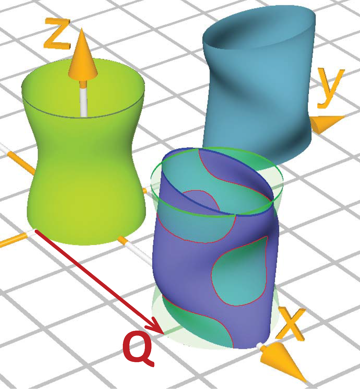
Figure 1: Schematic Fermi surface typical for iron pnictides showing only one hole band and two electron bands. Intersection between the hole Fermi surface displaced by the AF ordering wave vector $\mathbf{Q}$ and the electron Fermi surface marks the hot lines. Scattering by the AF fluctuations is enhanced at these lines.

Rich normal-state properties of iron-based high-temperature superconductors are caused by proximity to antiferromagnetic (AF) transition and multiple-band electronic structure.Paglione and Greene (2010); Stewart (2011); Shibauchi et al. (2014); Hosono and Kuroki (2015) AF fluctuations play important role in these materials and it is likely that superconductivity is mediated by these fluctuations. One can expect also that the spin fluctuations scatter quasiparticles in normal state and therefore influence transport properties. In particular, linear temperature dependence of resistivity near optimal doping Gooch et al. (2009); Kasahara et al. (2010) has been attributed to AF fluctuations near the quantum critical point. Such spin-fluctuations scattering is the strongest when momentum transfers are close to the AF instability vector $\mathbf{Q}$. As a consequence, scattering rate is strongly enhanced near so-called “hot lines” (or “hot spots” in quasi two-dimensional case), corresponding to ideal-nesting conditions for the vector $\mathbf{Q}$, see Fig. 1. The concept of hot spots has been introduced for cuprate high-temperature superconductors and their role in the transport properties has been considered in several theoretical papers Hlubina and Rice (1995); Stojkovic and Pines (1997); Löhneysen et al. (2007); Kontani (2008). For iron pnictides, the effects due to hot-spot scattering also has been discussed Fernandes et al. (2011); Breitkreiz et al. (2014a, b). In particular, the resistivity anisotropy induced by the orthorhombic deformation has been considered in Refs. Fernandes et al. (2011); Breitkreiz et al. (2014b). It was demonstrated that the hot-spot scattering mechanism provides a consistent description of the experimental anisotropy dependences on temperature and dopingBlomberg et al. (2013). In the related work Breitkreiz et al. (2013) the effects caused by interband scattering by AF fluctuations in metals with multiple isotropic bands have been investigated. Even though the hot lines are absent in this situation, it was demonstrated, nevertheless, that strong and anisotropic interband scattering leads to anomalous transport properties which are not described by the simple relaxation-time approximation.

The narrow hot lines do not strongly change conductivity which is determined by the average scattering time and therefore regular “cold” regions with weak scattering dominate.Hlubina and Rice (1995) However, the hot lines give the anomalous behavior of the conductivity in magnetic field Rosch (2000) including possible extended range of linear decrease with field. Such anomalies appear because the regions on the Fermi surface influenced by the hot lines grow with magnetic field. Similar mechanism also leads to unusual magnetic-field dependence of the Hall conductivity.

Electronic transport in the magnetic field has been investigated in detail practically for all families of iron-based superconductors spanning wide ranges of dopings Rullier-Albenque et al. (2009, 2010); Tsukada et al. (2010); Shen et al. (2011); Ohgushi and Kiuchi (2012); Eom et al. (2012); Sun et al. (2014); Li et al. (2014); Analytis et al. (2014); Moseley et al. (2015). The high-field magnetotransport in the paramagnetic state do exhibit several anomalous features such as linear magnetoresistance in Fe_1+yTe_0.6Se_0.4 Sun et al. (2014), nonquadratic magnetoresistance in optimally-doped Ba[As_1-xP_x]₂Fe₂ Analytis et al. (2014); Jia et al. and FeSeWatson et al. (2015), as well as the strongly nonlinear Hall resistance in FeTe_0.5Se_0.5Tsukada et al. (2010), Ba_0.5K_0.5As₂Fe₂ Li et al. (2014), FeSe Watson et al. (2015), and Ba[As_1-xP_x]₂Fe₂Jia et al. . These effects are likely to be caused by the hot-spot scattering due to the AF fluctuations. However, strong anisotropy of the spin-fluctuation scattering is frequently ignored and transport properties of the iron pnictides are interpreted using more conventional multiple-band Fermi-liquid theory Rullier-Albenque et al. (2009, 2010); Shen et al. (2011); Ohgushi and Kiuchi (2012); Watson et al. (2015) assuming that all scattering channels can be fully characterized by the band-dependent scattering rates.

Motivated by a clear relevance of the hot-spot mechanism for the iron pnictides and chalcogenides, we investigate in this paper transport properties of nearly-antiferromagnetic multiple-band metals. We consider in detail derivation of the collision integral for the Boltzmann equation and quasiparticle lifetime due to scattering by spin fluctuations. This allows us to relate the shape and strength of the hot-spot scattering rate with the microscopic parameters of the system. We proceed with analytical solution of the Boltzmann transport equation in the magnetic field using approximate transition rates which reproduce correctly physics of the hot-spot scattering. Our approach fully accounts for the return scattering events and therefore it is more accurate than the widely-used relaxation-time approximation. Based on the derived distribution functions, we compute the magnetic-field dependences of the longitudinal and Hall conductivities. These dependences are characterized by the two very different magnetic-field scales, the lower scale is set by the width of the hot spots and the higher scale is set by the total scattering amplitude. A conventional magnetotransport behavior is limited to the magnetic fields below the lower scale. In the wide field range in between these two scales the longitudinal conductivity has linear dependence on the magnetic field and the Hall conductivity has quadratic dependence. The linear dependence of the diagonal component reflects growth of the Fermi-surface area affected by hot spots proportional to the magnetic field. In the intermediate range the conductivity components are almost independent of the hot-spot parameters.

A somewhat similar behavior of magnetotransport is also realized in the antiferromagnetic state due to the Fermi surface reconstruction near the nesting points caused by opening of the antiferromagnetic gapFenton and Schofield (2005); Lin and Millis (2005); Koshelev (2013). The reconstructed Fermi surface acquires turning points at which the Fermi velocity changes abruptly. As a consequence, the longitudinal conductivity has linear dependence on the magnetic field Fenton and Schofield (2005); Koshelev (2013) and the Hall component has quadratic dependence Lin and Millis (2005) above the field scale set by the antiferromagnetic gap and scattering rate. In contrast to the hot-spot mechanism, for isolated turning points there is no higher magnetic field scale limiting this behavior from above.

This paper is organized as follows. In Sec. II we introduce the microscopic model describing two-band metal interacting with AF fluctuations. Based on this model, we present derivation of the collision integral in the Boltzmann equation in Sec. III. We analytically solve the Boltzmann equation using approximate scattering rates in Sec. IV. In Sec. V we compute conductivity in zero magnetic field. The conductivity components in magnetic field are considered in Sec. VI (longitudinal conductivity in subsection VI.1 and Hall conductivity in subsection VI.2). In Section VII we illustrate typical magnetic-field dependences of the conductivity components for a simple four-band model with two electron bands and two identical hole bands.

II Microscopic Model

For electronic band structure of iron-pnictides, the fluctuating AF magnetization mixes two bands, electron and hole. This means that for the treatment of an isolated hot line, it is sufficient to consider only a pair of interacting bands described by the following Hamiltonian

$$\mathcal{H}=\mathcal{H}_{0}+\mathcal{H}_{\mathrm{AF}},$$ (1)

where the free-electron part is composed of the electron and hole contributions,

$$\mathcal{H}_{0}=\sum_{\mathbf{p},\sigma}\left(\xi_{1,\mathbf{p}}c_{\mathbf{p}\sigma}^{\dagger}c_{\mathbf{p}\sigma}+\xi_{2,\mathbf{p}}d_{\mathbf{p}\sigma}^{\dagger}d_{\mathbf{p}\sigma}\right).$$ (2)

A particular shape of spectrum is not important for further consideration. In the electron part $\xi_{1,\mathbf{p}}$ the momentum $\mathbf{p}$ is measured with respect to the lattice wave vector $\mathbf{Q}$ at which the AF ordering takes place. The Fermi surfaces are determined by $\xi_{s,\mathbf{p}}=\mu$, where $\mu$ is the chemical potential. The hole Fermi surface and displaced electron Fermi surface cross along the hot lines, i.e., where $\xi_{1,\mathbf{p}}=\xi_{2,\mathbf{p}}$.

The antiferromagnetic part of the Hamiltonian is given by

$$\mathcal{H}_{\mathrm{AF}}\!=\!-\frac{g}{2}\!\sum_{\mathbf{p},\mathbf{p}^{\prime},j,\alpha,\beta}\!(M_{j,\mathbf{q}}\sigma_{\alpha\beta}^{j}c_{\mathbf{p}\alpha}^{\dagger}d_{\mathbf{p}^{\prime}\beta}\!+\!M_{j,-\mathbf{q}}\sigma_{\beta\alpha}^{j}d_{\mathbf{p}^{\prime}\beta}^{\dagger}c_{\mathbf{p}\alpha}),$$ (3)

where $M_{j,\mathbf{q}}$ are the magnetization components, $j=(x,y,z)$, $\mathbf{q}\!=\!\mathbf{p}\!-\!\mathbf{p}^{\prime}$ is the shift of the wave vector with respect to the AF-ordering vector $\mathbf{Q}$, and $\sigma_{\alpha\beta}^{j}$ are the Pauli matrices.

In paramagnetic state $\mathbf{M}_{\mathbf{q}}\equiv\tilde{\mathbf{M}}_{\mathbf{q}}(t)$ is the fluctuating magnetization which, in particular, scatters the carriers between the bands. According to the fluctuation-dissipation theorem, the amplitude of fluctuating magnetization $\left\langle\left|\tilde{M}_{j}(\mathbf{q},\omega)\right|^{2}\right\rangle$ is connected with the magnetic susceptibility $\chi_{j}(\mathbf{q},\omega)$ as

$$\left\langle\left|\tilde{M}_{j}(\mathbf{q},\omega)\right|^{2}\right\rangle=\frac{2T}{\omega}\operatorname{Im}\left[\chi_{j}(\mathbf{q},\omega)\right]$$ (4)

for $T\gg\omega$ (classical limit). The commonly used form of the susceptibility

$$\chi_{j}(\mathbf{q},\omega)=\frac{1}{-i\gamma\omega+\alpha_{j}+\eta_{i}q_{i}^{2}}$$ (5)

is valid for weak Gaussian magnetic fluctuations. In this case

$$\left\langle\left|\tilde{M}_{j}(\mathbf{q},\omega)\right|^{2}\right\rangle=\frac{2\gamma T}{\gamma^{2}\omega^{2}+\left(\alpha_{j}+\eta_{i}q_{i}^{2}\right)^{2}}.$$ (6)

The parameters $\alpha_{j}$ with $j=x,y,z$ characterize proximity to the magnetic transition temperature $T_{S}$. For continuous phase transition at least one of these parameters vanish at $T_{S}$. We mention that for continuous phase transitions the simple shape of the susceptibility (5) is not valid in the vicinity of the transition point, in the regime of strong critical fluctuations.

III Collision integral in Boltzmann equation and quasiparticle lifetime

Scattering of carriers are fully characterized by the collision integral in the Boltzmann equation Ziman (1960); Blatt (1968). The collision integral for scattering on the AF antiferromagnetic fluctuations was derived in Refs. Hlubina and Rice, 1995 and Rosch, 2000 for the two-dimensional and three-dimensional cases correspondingly. In this section, for completeness, we repeat its derivation for a three-dimensional multiband metal having in mind application to iron pnictides.

For the Hamiltonian (3) the collision integral due to scattering by the spin fluctuations is related to the dynamic spin susceptibility $\chi_{j}(\mathbf{q},\omega)$ as Hlubina and Rice (1995)

$$\mathcal{I}_{s}(\mathbf{p})\!=\!\frac{g^{2}}{2}\!\int\frac{d\mathbf{p}^{\prime}}{(2\pi)^{3}}\!\int\limits_{-\infty}^{\infty}\!d\omega\!\sum_{j}\operatorname{Im}\chi_{j}(\mathbf{q},\omega)\delta\left(\xi_{\bar{s},\mathbf{p}^{\prime}}\!-\!\xi_{s,\mathbf{p}}\!+\!\omega\right)$$

$$\times\left[-\!f_{s,\mathbf{p}}(1\!-\!f_{\bar{s},\mathbf{p}^{\prime}})(n(\omega)\!+\!1)\!+\!f_{\bar{s},\mathbf{p}^{\prime}}(1\!-\!f_{s,\mathbf{p}})n(\omega)\right],$$ (7)

where $f_{s,\mathbf{p}}$ is the distribution function for the fermions in band $s$, $\bar{s}\!=\!2(1)$ for $s\!=\!1(2)$, $\mathbf{q}=\mathbf{p}^{\prime}\!-\!\mathbf{p}$, and $n(\omega)=\left[\exp(\omega/T)-1\right]^{-1}$ is the Bose-Einstein distribution function. For small deviations from equilibrium, using standard presentation

$$f_{s,\mathbf{p}}=f_{s,\mathbf{p}}^{0}-\frac{\partial f_{s,\mathbf{p}}^{0}}{\partial\xi_{s,\mathbf{p}}}\Phi_{s,\mathbf{p}}=f_{s,\mathbf{p}}^{0}+\frac{f_{s,\mathbf{p}}^{0}\left(1-f_{s,\mathbf{p}}^{0}\right)}{T}\Phi_{s,\mathbf{p}},$$

we obtain

$$\mathcal{I}_{s}(\mathbf{p})\! =\!\frac{g^{2}}{2T}\!\int\frac{d\mathbf{p}^{\prime}}{(2\pi)^{3}}\int\limits_{-\infty}^{\infty}\!d\omega\sum_{j}\operatorname{Im}\chi_{j}(\mathbf{q},\omega)f_{s,\mathbf{p}}^{0}\left(1\!-\!f_{\bar{s},\mathbf{p}^{\prime}}^{0}\right)$$

$$\times \left[n(\omega)\!+\!1\right]\left(\Phi_{\bar{s},\mathbf{p}^{\prime}}-\Phi_{s,\mathbf{p}}\right)\delta\left(\xi_{s,\mathbf{p}}\!-\!\xi_{\bar{s},\mathbf{p}^{\prime}}\!-\!\omega\right),$$ (8)

where $f_{s,\mathbf{p}}^{0}=\left[\exp(\xi_{s,\mathbf{p}}/T)+1\right]^{-1}$ is the Fermi-Dirac distribution function.

The collision integral can be simplified using the standard transformation, $\int d\mathbf{p}^{\prime}\rightarrow\int\frac{dS_{\bar{s}}^{\prime}}{|v_{\bar{s}}^{\prime}|}\int d\xi_{\bar{s},\mathbf{p}^{\prime}}$, where $\int dS_{\bar{s}}^{\prime}\ldots$ means the integral over the Fermi surface of $\bar{s}$ band and $v_{\bar{s}}^{\prime}$ is the Fermi velocity for this band. Assuming that $\Phi_{\bar{s},\mathbf{p}^{\prime}}$ changes weakly on the scale $\xi_{\bar{s},\mathbf{p}^{\prime}}\sim T$, one can perform the energy integration independently, which allows us to reduce $\mathcal{I}_{s}(\mathbf{p})$ to the following form

$$\mathcal{I}_{s}(\mathbf{p}) =-\frac{g^{2}}{2(2\pi)^{3}}\!\frac{\partial f_{s,\mathbf{p}}^{0}}{\partial\xi_{s,\mathbf{p}}}$$

$$\times \int\frac{dS_{\bar{s}}^{\prime}}{|v_{\bar{s}}^{\prime}|}\left(\Phi_{\bar{s},\mathbf{p}^{\prime}}\!-\!\Phi_{s,\mathbf{p}}\right)\sum_{j}K_{j}(\mathbf{q},\xi_{s,\mathbf{p}})$$

with

$$K_{j}(\mathbf{q},\xi)=\int d\xi^{\prime}\operatorname{Im}\chi_{j}(\mathbf{q},\xi-\xi^{\prime})\frac{\cosh(\frac{\beta\xi}{2})}{2\cosh(\frac{\beta\xi^{\prime}}{2})\sinh\left[\frac{\beta\left(\xi\!-\!\xi^{\prime}\right)}{2}\right]},$$

where we used the following relations

$$\left[1\!-\!f^{0}(\xi^{\prime})\right]\left[n\left(\xi\!-\!\xi^{\prime}\right)+1\right]\!=\!\frac{\left[1\!-\!f^{0}(\xi)\right]\cosh(\frac{\beta\xi}{2})}{2\cosh(\frac{\beta\xi^{\prime}}{2})\sinh\left[\frac{\beta\left(\xi\!-\!\xi^{\prime}\right)}{2}\right]}$$

and $df^{0}/d\xi=-f^{0}(1-f^{0})/T$.

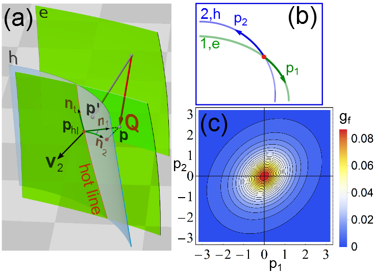
Figure 2: (a) Fermi-surface geometry near the hot line. Projection of the electron Fermi-surface section displaced by the AF wave vector $\mathbf{Q}$ intersects the hole section along the hot line. For scattering event, the initial momentum $\mathbf{p}$ is located at the displaced electron Fermi surface and final momentum $\mathbf{p}^{\prime}$ is located at the hole Fermi surface. The momentum $\mathbf{p}_{\mathrm{hl}}$ marks the location on the hot line closest to $\mathbf{p}$. (b) Cross sections of the hole and electron Fermi surfaces intersecting at the hot spot. The momenta $p_{s}$ with $s=1,2$ measure distances from the hot spot along the corresponding Fermi surfaces. (c) Representative contour plot of the transition rate $g_{\mathrm{f}}(p_{s},p_{\bar{s}})$, Eq. (11). We assumed that all $\alpha_{j}$ are identical and used the following parameters, $\eta_{1}=\eta_{2}$, $\eta_{12}=0.25\eta_{1}$, $(\pi/2)T\gamma=0.25\alpha$. $p_{s}$ and $g_{f}$ are measured in units of $\sqrt{\alpha/\eta_{1}}$ and $(3g^{2}T)/(16\pi\sqrt{\eta_{t}\alpha})$, respectively.

We consider a quasiparticle at the Fermi level, $\xi_{s,\mathbf{p}}=0$. In this case, with the shape of susceptibility given by Eq. (5), the energy integration reduces to calculation of the reduced integral

$$\zeta\left(a\right)=\int_{-\infty}^{\infty}du\frac{u}{a^{2}+u^{2}}\frac{1}{\sinh u}.$$

We can approximate this integral by the interpolation formula

$$\zeta\left(a\right)\approx\frac{\pi}{a(1+2a/\pi)},$$

which correctly reproduces its asymptotics. In this case $K_{j}(\mathbf{q},0)$ takes the following form

$$K_{j}(\mathbf{q},0)\approx\frac{\frac{\pi^{2}}{2}T^{2}\gamma}{\left(\alpha_{j}+\sum_{i}\eta_{i}q_{i}^{2}\right)(\frac{\pi}{2}T\gamma+\alpha_{j}+\sum_{i}\eta_{i}q_{i}^{2})},$$

and we obtain a useful intermediate result for the collision integral

$$\mathcal{I}_{s}(\mathbf{p})\!\approx\!-\frac{g^{2}}{2(2\pi)^{3}}\!\frac{\partial f_{s,\mathbf{p}}^{0}}{\partial\xi_{s,\mathbf{p}}}$$

$$\times\sum_{j}\int\frac{dS_{\bar{s}}^{\prime}}{|v_{\bar{s}}^{\prime}|}\frac{\frac{\pi^{2}}{2}T^{2}\gamma\left(\Phi_{\bar{s},\mathbf{p}^{\prime}}-\Phi_{s,\mathbf{p}}\right)}{\left(\alpha_{j}\!+\!\sum_{i}\eta_{i}q_{i}^{2}\right)(\frac{\pi}{2}T\gamma+\alpha_{j}\!+\!\sum_{i}\eta_{i}q_{i}^{2})},$$ (9)

which contains two-dimensional integration over the Fermi surface. Further simplification can be done observing that $\Phi_{\bar{s},\mathbf{p}^{\prime}}$ strongly depends on the distance between $\mathbf{p}^{\prime}$ and the hot line but varies smoothly along this line. Therefore one can perform integration over the component $\mathbf{p}^{\prime}$ along the hot line neglecting the dependence of $\Phi_{\bar{s},\mathbf{p}^{\prime}}$ on this component Rosch (2000). This integration in general case, however, is somewhat complicated by the anisotropy of the susceptibility characterized by the parameters $\eta_{i}$. To proceed, we introduce the unit vector along the hot line $\mathbf{n}_{t}$ and the unit vectors along the electron and hole Fermi surfaces $\mathbf{n}_{s}$ with $s=1,2$ satisfying the conditions $\sum_{i}\eta_{i}n_{t,i}n_{s,i}=0$, which replace the orthogonality conditions in the isotropic case. Geometry around the hot line is illustrated in Fig. 2(a). We can now decompose the momenta $\mathbf{p}$ and $\mathbf{p}^{\prime}$ as $\mathbf{p}=\mathbf{p}_{\mathrm{hl}}+\mathbf{n}_{s}p_{s}$, $\mathbf{p}^{\prime}=\mathbf{p}_{\mathrm{hl}}+\mathbf{n}_{t}p_{t}+\mathbf{n}_{\bar{s}}p_{\bar{s}}$, where $\mathbf{p}_{\mathrm{hl}}$ is the hot-line momentum closest to $\mathbf{p}$ and $p_{t}$ is the component of $\mathbf{p}^{\prime}$ along the hot-line. The momentum components $p_{s}$ measure distance to the hot line, see Fig. 2(b). With such a decomposition, the sum $\sum_{i}\eta_{i}q_{i}^{2}$ takes the following form

$$\sum_{i}\eta_{i}q_{i}^{2}=\sum_{i}\eta_{i}\left(p_{i}-p_{i}^{\prime}\right)^{2}=\eta_{t}p_{t}^{2}+\eta_{s}p_{s}^{2}+\eta_{\bar{s}}p_{\bar{s}}^{2}-2\eta_{s\bar{s}}p_{s}p_{\bar{s}}$$

with

$$\eta_{t}=\sum_{i}\eta_{i}n_{t,i}^{2},\ \eta_{s}=\sum_{i}\eta_{i}n_{s,i}^{2},\text{and }\eta_{s,\bar{s}}=\sum_{i}\eta_{i}n_{s,i}n_{\bar{s},i}.$$

As the distribution function $\Phi_{\bar{s},\mathbf{p}^{\prime}}$ only weakly depends on the parallel momentum $p_{t}$, we can neglect this dependence, $\Phi_{\bar{s},\mathbf{p}^{\prime}}\rightarrow\Phi_{\bar{s}}(p_{\bar{s}})$, and perform integration over $p_{t}$ in $\mathcal{I}_{s}(\mathbf{p})$ which leads us to the following final presentation of the collision integral

$$\mathcal{I}_{s}(p_{s})\!\approx\!-\!\frac{\partial f_{s,\mathbf{p}}^{0}}{\partial\xi_{s,\mathbf{p}}}\int\frac{dp_{\bar{s}}}{|v_{\bar{s}}|}g_{\mathrm{f}}(p_{s},p_{\bar{s}})\left[\Phi_{\bar{s}}(p_{\bar{s}})-\Phi_{s}(p_{s})\right]$$ (10)

with

$$g_{\mathrm{f}}(p_{s},p_{\bar{s}}) =\frac{g^{2}T}{16\pi\sqrt{\eta_{t}}}\sum_{j}\left(\frac{1}{\sqrt{\alpha_{j}\!+\!u(p_{s},p_{\bar{s}})}}\right.$$

$$- \left.\frac{1}{\sqrt{\frac{\pi}{2}T\gamma\!+\!\alpha_{j}\!+\!u(p_{s},p_{\bar{s}})}}\right),$$ (11)

$$u(p_{s},p_{\bar{s}}) =\eta_{s}p_{s}^{2}+\eta_{\bar{s}}p_{\bar{s}}^{2}-2\eta_{s\bar{s}}p_{s}p_{\bar{s}}.$$

The transition rate $g_{\mathrm{f}}(p_{s},p_{\bar{s}})$ increases as both the initial and final momenta approach the hot line, $p_{s},p_{\bar{s}}\rightarrow 0$. Its shape is determined by the parameters of dynamic susceptibility, $\alpha_{j}$, $\eta_{i}$, and $\gamma$, see Eq. (5). The first term in parentheses in Eq. (11) describes elastic scattering by static “snapshots” of the fluctuating magnetization, while the second term gives dynamic inelastic contribution. The typical behavior of $g_{\mathrm{f}}(p_{s},p_{\bar{s}})$ is illustrated by the contour plot in Fig. 2(c). Equations (10) and (11) give the simplest accurate presentation for the collision integral which can be used for precise numerical calculations of transport properties.

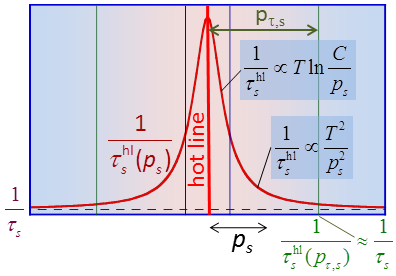
Figure 3: Behavior of the quasiparticle lifetime, Eq. (12), near the hot line.

The intensity of scattering near the hot line can be characterized by the quasiparticle lifetime $\tau_{s}^{\mathrm{hl}}(p_{s})$,

$$\frac{1}{\tau_{s}^{\mathrm{hl}}}(p_{s}) =\int\frac{dp_{\bar{s}}}{|v_{\bar{s}}|}g_{\mathrm{f}}(p_{s},p_{\bar{s}})$$

$$=\frac{g^{2}T}{16\pi\sqrt{\eta_{t}\eta_{\bar{s}}}|v_{\bar{s}}|}\sum_{j}\ln\left(1+\frac{\frac{\pi}{2}T\gamma}{\alpha_{j}+\widetilde{\eta}_{s}p_{s}^{2}}\right)$$ (12)

with

$$\widetilde{\eta}_{s}\equiv\frac{\eta_{s}\eta_{\bar{s}}-\eta_{s\bar{s}}^{2}}{\eta_{\bar{s}}}.$$

Behavior of the quasiparticle lifetime near the hot line is illustrated in Fig. 3. One can see that there are two regimes of scattering, depending on the temperature and proximity to the hot line. For $\gamma T\ll\widetilde{\eta}_{s}p_{s}^{2}$ the scattering rate behaves as $1/\tau_{s}^{\mathrm{hl}}\propto T^{2}/p_{s}^{2}$. For $\gamma T\gg\widetilde{\eta}_{s}p_{s}^{2}$ the scattering rate grows logarithmically $1/\tau_{s}^{\mathrm{hl}}\propto T/\ln(C/|p_{s}|)$ and saturates at $|p_{s}|=\sqrt{\alpha_{j}/\widetilde{\eta}_{s}}$. In the latter regime the frequency dependence of the susceptibility is not essential meaning that this regime corresponds to scattering on static “frozen” AF fluctuations. In general, the $\eta$-parameters depend on local orientation of the hot line. For common particular case of hot line oriented along the $z$ axis and no in-plane anisotropy, $\eta_{x}=\eta_{y}$, we have simple relations $\eta_{t}=\eta_{z}$, $\eta_{s}=\eta_{\bar{s}}=\eta_{x}$, $\eta_{s\bar{s}}=\eta_{x}\cos\alpha_{\mathrm{eh}}$, and $\widetilde{\eta}_{s}=\eta_{x}\sin^{2}\alpha_{\mathrm{eh}}$, where $\alpha_{\mathrm{eh}}$ is the angle between the electron and hole Fermi surfaces. In this case $u(p_{s},p_{\bar{s}})$ in Eq. (11) is just proportional to the momentum change squared, $u(p_{s},p_{\bar{s}})=\eta_{x}(p_{s}\mathbf{n}_{s}-p_{\bar{s}}\mathbf{n}_{\bar{s}})^{2}$.

IV Solution of Boltzmann equation using approximate transition rates.

To obtain conductivity in magnetic field, one has to solve the Boltzmann kinetic equation for the distribution function Ziman (1960); Blatt (1968). We assume that the electric field $\mathbf{E}$ is applied in the $xy$ plane and the magnetic field $H$ applied along $z$ axis. Using simplified collision integral, Eqs. (10) and (11), the two-band Boltzmann equation takes the following approximate form

$$- eE_{\alpha}v_{s,\alpha}-\frac{e}{c}Hv_{s}\frac{d\Phi_{s,\alpha}}{dp_{s}}\!=\!-\frac{\Phi_{s,\alpha}}{\tau_{s}}$$

$$+\int\frac{dp_{s}}{|v_{s}|}g_{\mathrm{f}}(p_{s},p_{\bar{s}})\left[\Phi_{\bar{s},\alpha}(p_{\bar{s}})-\Phi_{s,\alpha}(p_{s})\right],$$ (13)

where $\tau_{s}$ are the background scattering times, which we assume to be isotropic. We remind that in our notations $s=1$ corresponds to the electron band, $v_{1}>0$, and $s=2$ corresponds to the hole band, $v_{2}<0$. Equation (13) represents a system of coupled one-dimensional integro-differential equations for the distribution functions depending on distances from the hot spot $p_{s}$, see Fig. 2(b). These equations do not have exact analytical solution. Therefore, one can either solve them numerically or rely on some approximations. The most common approach is the relaxation-time approximation within which the return scattering events described by the term $\int\frac{dp_{s}}{|v_{s}|}g(p_{s},p_{\bar{s}})\Phi_{\bar{s},\alpha}(p_{\bar{s}})$ are completely neglected. Even though in most cases this approximation gives physically reasonable predictions, for strongly anisotropic scattering, it is not quantitatively accurate Kontani (2008); Breitkreiz et al. (2014a). Alternatively, the precise solution of the kinetic equation can be obtained numerically. We propose a different approximate scheme, which also allows for exact analytical solution and preserves several realistic properties of the system which are lost in the relaxation-time model. We will replace the exact transition rates (11) with the approximate factorizable form

$$g_{\mathrm{f}}(p_{1},p_{2})\!=\!\gamma_{\mathrm{hs}}\psi_{1}(p_{1})\psi_{2}(p_{2}),$$ (14)

where the functions $\psi_{s}(p_{s})$ are normalized as

$$\int_{-\infty}^{\infty}\frac{dp_{s}}{|v_{s}|}\psi_{s}(p_{s})=1$$

and their shapes are chosen to reproduce the hot-line relaxation time (12),

$$\frac{1}{\tau_{s}^{\mathrm{hl}}(p_{s})}=\gamma_{\mathrm{hs}}\psi_{s}(p_{s}).$$ (15)

Therefore, the total amplitude characterizing the strength of hot-spot scattering is given by

$$\gamma_{\mathrm{hs}}=\int\frac{dp_{s}}{|v_{s}|}\frac{1}{\tau_{s}^{\mathrm{hl}}(p_{s})}=\int\frac{dp_{1}}{v_{1}}\int\frac{dp_{2}}{|v_{2}|}g_{\mathrm{f}}(p_{1},p_{2}).$$

The relative strength of the hot spot with respect to background scattering can be conveniently characterized by the reduced parameter $\gamma_{\mathrm{hs}}|v_{s}|\tau_{s}/p_{F,s}$. We will assume that this parameter is small.

Introducing notations

$$\Phi_{s,\alpha}(p_{s})\!=\!eE_{\alpha}\Lambda_{s,\alpha}(p_{s}),$$ (16a)

$$\bar{\Lambda}_{s,\alpha}\!=\!\int\frac{dp_{s}}{|v_{s}|}\psi_{s}(p_{s})\Lambda_{s,\alpha}(p_{s}),$$ (16b)

we obtain from Eq. (13) the following equation for the “vector mean-free path”Taylor (1963) $$\Lambda_{s,\alpha}(p_{s})$$

$$\left[\frac{1}{\tau_{s}}\!+\!\gamma_{\mathrm{hs}}\psi_{s}(p_{s})\right]\Lambda_{s,\alpha}\!-\!\frac{e}{c}Hv_{s}\frac{d\Lambda_{s,\alpha}}{dp_{s}}\!=\!v_{s,\alpha}\!+\!\gamma_{\mathrm{hs}}\psi_{s}(p_{s})\bar{\Lambda}_{\bar{s},\alpha}.$$ (17)

The conductivity tensor is related to $\Lambda_{s,\alpha}(p_{s})$ as

$$\sigma_{\alpha\beta} =\frac{2e^{2}}{(2\pi)^{3}}\int dp_{z}S_{\alpha\beta},$$ (18a)

$$S_{\alpha\beta} \approx\sum_{s}\int\frac{dp_{s}}{|v_{s}|}v_{s,\alpha}\Lambda_{s,\beta}.$$ (18b)

The physical parameters $$v_{s} \gamma_{\mathrm{hs}} z p_{z} p_{z} p_{z} p_{z} \sigma_{\alpha\beta}^{\mathrm{hl}}$$ and entering Eq. (17) depend on axis momentum as an external parameter. Therefore this equation deals with fixed- cross section of the Fermi surface which intersects hot lines at the hot spots. The total conductivity is obtained by integration over . In the following, we will skip an implicit dependence on in all parameters. The hot-line contribution to the conductivity, , is given by

$$\sigma_{\alpha\beta}^{\mathrm{hl}}=\frac{2e^{2}}{(2\pi)^{3}}\int dp_{z}\sum_{\mathrm{hs}}S_{\alpha\beta}^{\mathrm{hs}},$$ (19)

where $S_{\alpha\beta}^{\mathrm{hs}}$ is the contribution to $S_{\alpha\beta}$ from one hot spot and the sum is taken over all hot spots in the given $p_{z}$ cross section. In the following sections we solve Eq. (17) and compute components of conductivity.

V Conductivity in zero magnetic field

For completeness, we consider first the conductivity at zero magnetic field, see also Ref. Stojkovic and Pines, 1997. Rewriting Eq. (17) as

$$\Lambda_{s,\alpha}\!=\!\frac{v_{s,\alpha}}{\frac{1}{\tau_{s}}+\gamma_{\mathrm{hs}}\psi_{s}(p_{s})}+\frac{\gamma_{\mathrm{hs}}\psi_{s}(p_{s})}{\frac{1}{\tau_{s}}+\gamma_{\mathrm{hs}}\psi_{s}(p_{s})}\bar{\Lambda}_{\bar{s},\alpha},$$

we obtain $2\times 2$ linear system for $\bar{\Lambda}_{s,\alpha}$ defined by Eq. (16b)

$$\bar{\Lambda}_{1,\alpha}-\left(1-r_{1}\right)\bar{\Lambda}_{2,\alpha}\! =r_{1}\tau_{1}v_{1,\alpha}^{\mathrm{hs}},$$ (20a)

$$-\left(1-r_{2}\right)\bar{\Lambda}_{1,\alpha}+\bar{\Lambda}_{2,\alpha}\! =r_{2}\tau_{2}v_{2,\alpha}^{\mathrm{hs}},$$ (20b)

where $$v_{s,\alpha}^{\mathrm{hs}} r_{s}$$ are Fermi-velocity components at the hot spot and the dimensionless parameters are defined as

$$r_{s}\equiv\int\!\frac{\psi_{s}(p_{s})dp_{s}/|v_{s}|}{1+\tau_{s}\gamma_{\mathrm{hs}}\psi_{s}(p_{s})}=\frac{1}{\gamma_{\mathrm{hs}}}\int\!\frac{dp_{s}/|v_{s}|}{\tau_{s}+\tau_{s}^{\mathrm{hl}}(p_{s})}.$$ (21)

The solution of these equations is

$$\bar{\Lambda}_{s,\alpha}=\frac{r_{s}\tau_{s}v_{s,\alpha}^{\mathrm{hs}}+r_{\bar{s}}\left(1-r_{s}\right)\tau_{\bar{s}}v_{\bar{s},\alpha}^{\mathrm{hs}}}{r_{1}+r_{2}-r_{1}r_{2}}.$$ (22)

In the case of narrow hot spot, $r_{s}\ll 1$, we obtain the following approximate result for the vector mean-free path

$$\Lambda_{s,\alpha}(p_{s})\!\approx\frac{r_{1}v_{1,\alpha}^{\mathrm{hs}}\tau_{1}+r_{2}v_{2,\alpha}^{\mathrm{hs}}\tau_{2}}{r_{1}+r_{2}}$$

$$+\frac{1}{1\!+\!\tau_{s}/\tau_{s}^{\mathrm{hl}}(p_{s})}\left(v_{s,\alpha}\tau_{s}\!-\frac{r_{1}v_{1,\alpha}^{\mathrm{hs}}\tau_{1}\!+\!r_{2}v_{2,\alpha}^{\mathrm{hs}}\tau_{2}}{r_{1}+r_{2}}\right).$$ (23)

Here the first term approximately gives the vector mean-free path in the hot-spot region. Due to strong equilibration, it is identical for two bands. This result can also be rewritten approximately as

$$\Lambda_{s,\alpha}(p_{s})\!\approx v_{s,\alpha}\tau_{s}\!+\!\frac{\tau_{s}}{\tau_{s}\!+\!\tau_{s}^{\mathrm{hl}}(p_{s})}\frac{\left(v_{\bar{s},\alpha}^{\mathrm{hs}}\tau_{\bar{s}}\!-v_{s,\alpha}^{\mathrm{hs}}\tau_{s}\right)r_{\bar{s}}}{r_{1}+r_{2}}.$$ (24)

We can see that far away from the hot spot where $\tau_{s}^{\mathrm{hl}}(p_{s})\gg\tau_{s}$, the conventional result $\Lambda_{s,\alpha}(p_{s})\approx v_{s,\alpha}\tau_{s}$ is restored. The transition to this asymptotic takes place at the typical momentum $p_{\tau,s}$ where the hot-spot scattering rate drops down to the background, $\tau_{s}^{\mathrm{hl}}(p_{\tau,s})=\tau_{s}$, see Fig. 3. Note that this typical momentum is mostly determined by the tail region in the scattering rate $1/\tau_{s}^{\mathrm{hl}}(p_{s})$ and changes only weakly when the temperature approaches the transition point.

Substituting result from Eq. (24) into Eq. (18b), we obtain

$$S_{\alpha\alpha}=S_{\alpha\alpha}^{(0)}+S_{\alpha\alpha}^{\mathrm{hs}},$$ (25a)

with the background and hot-spot contributions given by

$$S_{\alpha\alpha}^{(0)} =\sum_{s}\int v_{s,\alpha}^{2}\tau_{s}\frac{dp_{s}}{|v_{s}|},$$ (25b)

$$S_{\alpha\alpha}^{\mathrm{hs}} =-\gamma_{\mathrm{hs}}\frac{\left(v_{2,\alpha}^{\mathrm{hs}}\tau_{2}-v_{1,\alpha}^{\mathrm{hs}}\tau_{1}\right)^{2}}{1/r_{1}+1/r_{2}}.$$ (25c)

Remind that $$S_{\alpha\alpha} \sigma_{\alpha\alpha} \tau_{s}^{\mathrm{hl}}(p_{s})$$ directly determines the conductivity by Eq. (18a). Alternatively, the hot-spot contribution can be expressed via the relaxation rates ,

$$S_{\alpha\alpha}^{\mathrm{hs}}=-\left(v_{2,\alpha}^{\mathrm{hs}}\tau_{2}-v_{1,\alpha}^{\mathrm{hs}}\tau_{1}\right)^{2}\left\{\sum_{s}\left[\int\!\frac{dp_{s}/|v_{s}|}{\tau_{s}+\tau_{s}^{\mathrm{hl}}(p_{s})}\right]^{-1}\right\}^{-1}$$

and can be estimated as

$$S_{\alpha\alpha}^{\mathrm{hs}}\approx-\frac{\left(v_{2,\alpha}^{\mathrm{hs}}\tau_{2}-v_{1,\alpha}^{\mathrm{hs}}\tau_{1}\right)^{2}}{\frac{\tau_{1}|v_{1}|}{p_{\tau,1}}+\frac{\tau_{2}|v_{2}|}{p_{\tau,2}}}.$$

Typically, the cold regions dominate in transport and the hot spots give only small corrections Stojkovic and Pines (1997). Moreover, these corrections are not singular at the transition point. As the carriers within the range $\sim p_{\tau}$ from the hot line are almost eliminated from transport, the relative reduction of conductivity is of the order of $\sigma_{\alpha\alpha}^{\mathrm{hs}}/\sigma_{\alpha\alpha}^{(0)}\approx p_{\tau}/p_{F}$. Note, however, that, contrary to the relaxation-time approximation, in the case $r_{1}v_{1,\alpha}^{\mathrm{hs}}\tau_{1}+r_{2}v_{2,\alpha}^{\mathrm{hs}}\tau_{2}\neq 0$, the distribution functions do not vanish in the hot-spot regions and therefore these regions actually give finite contributions to the current and conductivity.

VI Conductivity in magnetic field

In the magnetic field the formal solution of Eq. (17) can be written as

$$\Lambda_{s,\alpha}(p_{s})\!=\!\int\limits_{p_{s}}^{\delta_{s}\infty}\!\frac{dp_{s}^{\backprime}}{v_{s}^{\backprime}}\frac{v_{s,\alpha}^{\backprime}\!+\!\gamma_{\mathrm{hs}}\psi_{s}(p_{s}^{\backprime})\bar{\Lambda}_{\bar{s},\alpha}}{\frac{e}{c}H}\mathcal{L}_{H,s}(p_{s}^{\backprime},p_{s}),$$ (26a)

$$\mathcal{L}_{H,s}(p_{s}^{\backprime},p_{s})\equiv\exp\left[-\int_{p_{s}}^{p_{s}^{\backprime}}\frac{\frac{1}{\tau_{s}}+\gamma_{\mathrm{hs}}\psi_{s}(\tilde{p}_{s})}{\frac{e}{c}H}\frac{d\tilde{p}_{s}}{\tilde{v}_{s}}\right]$$ (26b)

with $$\delta_{s}\equiv\mathrm{sgn}(ev_{s})\equiv-\mathrm{sgn}(v_{s}) p_{s}^{\backprime} p_{s} \bar{\Lambda}_{\bar{s},\alpha}$$. This presentation is similar to so-called Shockley “tube integral”Shockley (1950), see also Ref. Abdel-Jawad et al., 2006 for the recent use of this approach. The exponent in Eq. (26b) is the probability of reaching point from point without scattering during orbital motion of quasiparticle in the magnetic field. The term with in Eq. (26a) describes the contribution from the return-scattering events. Without this term Eq. (26a) would give the relaxation-time-approximation result. Using the identity

$$\int_{p_{s}}^{\delta_{s}\infty}\!\frac{dp_{s}^{\backprime}}{v_{s}^{\backprime}}\frac{\frac{1}{\tau_{s}}+\gamma_{\mathrm{hs}}\psi_{s}(p_{s}^{\backprime})}{\frac{e}{c}H}\mathcal{L}_{H,s}(p_{s}^{\backprime},p_{s})=1,$$

we can also transform this presentation to the following form

$$\Lambda_{s,\alpha}(p_{s})\!=\!\bar{\Lambda}_{\bar{s},\alpha}+\int\limits_{p_{s}}^{\delta_{s}\infty}\!dp_{s}^{\backprime}\frac{\tau_{s}v_{s,\alpha}^{\backprime}-\bar{\Lambda}_{\bar{s},\alpha}}{\frac{e}{c}Hv_{s}^{\backprime}\tau_{s}}\mathcal{L}_{H,s}(p_{s}^{\backprime},p_{s}).$$ (27)

From this result, we derive the linear system for the parameters $\bar{\Lambda}_{s,\alpha}$,

$$\bar{\Lambda}_{s,\alpha}\!-\left(1-R_{s}\right)\bar{\Lambda}_{\bar{s},\alpha}=\!\mathcal{V}_{s,\alpha}\tau_{s},$$ (28)

where the parameters $R_{s}$ and $\mathcal{V}_{s,\alpha}$ are defined by the double integrals,

$$R_{s}=\!\frac{1}{\tau_{s}\gamma_{\mathrm{hs}}}\int\limits_{-\infty}^{\infty}\frac{dp_{s}^{\backprime}}{|v_{s}^{\backprime}|}\!\int\limits_{-\delta_{s}\infty}^{p_{s}^{\backprime}}\!\frac{dp_{s}}{\frac{e}{c}H\tau_{s}v_{s}}\mathcal{M}_{H,s}(p_{s}^{\backprime},p_{s})$$ (29a)

and

$$\mathcal{V}_{s,\alpha}\!=\!\frac{1}{\tau_{s}\gamma_{\mathrm{hs}}}\!\int\limits_{-\infty}^{\infty}\!v_{s,\alpha}^{\backprime}\frac{dp_{s}^{\backprime}}{|v_{s}^{\backprime}|}\!\int\limits_{-\delta_{s}\infty}^{p_{s}^{\backprime}}\!\frac{dp_{s}}{\frac{e}{c}H\tau_{s}v_{s}}\mathcal{M}_{H,s}(p_{s}^{\backprime},p_{s})$$ (29b)

with

$$\mathcal{M}_{H,s} (p_{s}^{\backprime},p_{s})\equiv\exp\left(\!-\!\int_{p_{s}}^{p_{s}^{\backprime}}\frac{d\tilde{p}_{s}}{\frac{e}{c}H\tau_{s}\tilde{v}_{s}}\right)$$

$$\times \left[1-\exp\left(-\frac{\gamma_{\mathrm{hs}}}{\frac{e}{c}H}\int_{p_{s}}^{p_{s}^{\backprime}}\!\psi_{s}(\tilde{p}_{s})\frac{d\tilde{p}_{s}}{\tilde{v}_{s}}\right)\right].$$ (29c)

The solution of Eq. (28) is

$$\bar{\Lambda}_{s,\alpha}=\frac{\!\mathcal{V}_{s,\alpha}\tau_{s}+\mathcal{V}_{\bar{s},\alpha}\tau_{\bar{s}}\left(1-R_{s}\right)}{R_{1}+R_{2}-R_{1}R_{2}}.$$ (30)

This result determines the vector mean-free path by Eq. (27), which, in turn, determines the conductivity components by Eqs. (18a) and (18b). In the following sections we proceed with the derivation of the longitudinal and Hall conductivities.

VI.1 Longitudinal conductivity

For calculation of the longitudinal conductivity, in the integral for $\mathcal{V}_{s,\alpha}$, Eq. (29b), one can replace $v_{s,\alpha}^{\backprime}$ by its value at the hot line, $v_{s,\alpha}^{\mathrm{hs}}$, giving $\mathcal{V}_{s,\alpha}\approx v_{s,\alpha}^{\mathrm{hs}}R_{s}$. To proceed further, we need to obtain a tractable expression for the field-dependent parameter $R_{s}(H)$, Eqs. (29a) and (29c). The essential magnetic field scale in this dependence, $B_{w,s}$, is set by the typical width of the hot spot scattering rate $w_{s}\approx\sqrt{\alpha_{j}/\widetilde{\eta}_{s}}$ (the width of the functions $\psi_{s}(p_{s})$) as

$$B_{w,s}=\frac{c}{|e|}\sqrt{\frac{\pi\gamma_{\mathrm{hs}}w_{s}}{|v_{s}^{\mathrm{hs}}|\tau_{s}}}.$$ (31)

While behavior at very small magnetic fields, $H\ll B_{w,s}$, is sensitive to exact shape of $\psi_{s}(p_{s})$, at higher fields the internal structure of $\psi_{s}(p_{s})$ is not important and it can be treated as $\delta$-functions, $\psi_{s}(p_{s})\rightarrow|v_{s}|\delta(p_{s})$. This allows us to derive relatively simple analytical results for this magnetic field regime. In this case, we obtain that the parameters $R_{s}$, Eq. (29a), are identical for both bands and given by

$$R_{s}\approx\frac{H}{B_{\gamma}}\left[1\!-\!\exp\left(-\frac{B_{\gamma}}{H}\right)\right]$$ (32)

with the field scale

$$B_{\gamma}=\frac{c}{|e|}\gamma_{\mathrm{hs}}$$ (33)

set by the total scattering amplitude. The exponential factor in this result represents probability for a quasiparticle to pass through the hot spot without scattering. For $H\ll B_{\gamma}$ this probability is negligibly small. Substituting result (32) into Eqs. (30), we obtain

$$\bar{\Lambda}_{s,\alpha}\!\approx\!\frac{v_{s,\alpha}^{\mathrm{hs}}\tau_{s}+v_{\bar{s},\alpha}^{\mathrm{hs}}\tau_{\bar{s}}\left\{1-\frac{H}{B_{\gamma}}\left[1\!-\!\exp\left(-\frac{B_{\gamma}}{H}\right)\right]\right\}}{\!2\!-\!\frac{H}{B_{\gamma}}\left[1\!-\!\exp\left(-\frac{B_{\gamma}}{H}\right)\right]}$$

and from Eq. (27) the vector mean-free path

$$\Lambda_{s,\alpha}(p_{s})\!\approx\!v_{s,\alpha}\tau_{s}-\left(v_{s,\alpha}^{\mathrm{hs}}\tau_{s}-v_{\bar{s},\alpha}^{\mathrm{hs}}\tau_{\bar{s}}\right)\theta(-\delta_{s}p_{s})$$

$$\times\exp\left(\frac{p_{s}}{\frac{e}{c}Hv_{s}^{\mathrm{hs}}\tau_{s}}\right)\frac{1\!-\!\exp\left(-\frac{B_{\gamma}}{H}\right)}{2\!-\!\frac{H}{B_{\gamma}}\left[1\!-\!\exp\left(-\frac{B_{\gamma}}{H}\right)\right]},$$ (34)

where $\theta(x)$ is the step function. We can see that the hot spot affects the distribution function only on one side, in the range $\Delta_{H}p_{s}=\frac{e}{c}H|v_{s}^{\mathrm{hs}}|\tau_{s}$, meaning that the affected area of the Fermi surface grows proportionally to the magnetic field. This result also means that the hot spots influence conductivity independently until $\Delta_{H}p_{s}<p_{F,s}$. Substituting derived $\Lambda_{s,\alpha}(p_{s})$ into Eq. (18b), we obtain the magnetic-field dependent part of $S_{\alpha\alpha}^{\mathrm{hs}}(H)$, $\delta S_{\alpha\alpha}^{\mathrm{hs}}(H)\equiv S_{\alpha\alpha}^{\mathrm{hs}}(H)-\!S_{\alpha\alpha}^{\mathrm{hs}}(0)$,

$$\delta S_{\alpha\alpha}^{\mathrm{hs}}(H)\!\approx\!-\left(v_{1,\alpha}^{\mathrm{hs}}\tau_{1}\!-\!v_{2,\alpha}^{\mathrm{hs}}\tau_{2}\right)^{2}\!\frac{\frac{e}{c}H\left[1\!-\!\exp\left(-\frac{B_{\gamma}}{H}\right)\right]}{2\!-\!\frac{H}{B_{\gamma}}\left[1\!-\!\exp\left(-\frac{B_{\gamma}}{H}\right)\right]},$$ (35)

meaning that the reduction of conductivity due hot-line scattering increases linearly with the magnetic field within $B_{w,s}<H<B_{\gamma}$,

$$\delta S_{\alpha\alpha}^{\mathrm{hs}}\approx-\frac{1}{2}\left(v_{1,\alpha}^{\mathrm{hs}}\tau_{1}\!-\!v_{2,\alpha}^{\mathrm{hs}}\tau_{2}\right)^{2}\frac{e}{c}H.$$ (36)

In this linear regime the penetration of a carrier through the hot spot without scattering is negligible and the conductivity is not sensitive to the hot-spot parameters at all. At higher field, $H>B_{\gamma}$, the hot-spot contribution saturates at a finite value,

$$\delta S_{\alpha\alpha}^{\mathrm{hs}}\!\approx\!-\gamma_{\mathrm{hs}}\left(v_{1,\alpha}^{\mathrm{hs}}\tau_{1}\!-\!v_{2,\alpha}^{\mathrm{hs}}\tau_{2}\right)^{2}.$$ (37)

This result is valid assuming that the hot spots still act independently at $H\sim B_{\gamma}$, which is correct if $B_{\gamma}<(c/e)p_{F,s}/|v_{s}|\tau_{s}$ corresponding to the condition for the hot-spot strength $\gamma_{\mathrm{hs}}<p_{F,s}/|v_{s}|\tau_{s}$.

For quantitative description of the behavior in the full field range including $B\sim B_{w,s}$, we assume a simple Lorentzian shape of $\psi_{s}(p_{s})$ valid for $T<\alpha_{j}/\gamma$, see Eq. (12), and close $\alpha_{j}$ for all $j$,

$$\psi_{s}(p_{s})=\frac{|v_{s}^{\mathrm{hs}}|w_{s}/\pi}{p_{s}^{2}+w_{s}^{2}}.$$ (38)

Comparing with microscopic result, Eq. (12), we can express the strength and width of the hot spot via the microscopic parameters as

$$\gamma_{\mathrm{hs}}=\frac{3\pi g^{2}\gamma T^{2}}{32|v_{\bar{s}}||v_{s}|\sqrt{\eta_{t}\left(\eta_{s}\eta_{\bar{s}}-\eta_{s\bar{s}}^{2}\right)\alpha_{x}}},\ w_{s}=\sqrt{\frac{\alpha_{x}}{\tilde{\eta}_{s}}}.$$ (39)

In this case, for $w_{s}\ll\gamma_{\mathrm{hs}}\tau_{s}|v_{s}^{\mathrm{hs}}|/\pi$, the parameter $r_{s}$, Eq. (21), can be evaluated as

$$r_{s}\approx\sqrt{\frac{\pi w_{s}}{\gamma_{\mathrm{hs}}|v_{s}^{\mathrm{hs}}|\tau_{s}}}.$$ (40)

Note that this parameter also determines the ratio of the typical fields $B_{w,s}$ and $B_{\gamma}$, $B_{w,s}=r_{s}B_{\gamma}$. The typical momentum scale $p_{\tau,s}$ defined in the previous section by the condition $\tau_{s}^{\mathrm{hl}}(p_{\tau,s})=\tau_{s}$ becomes $p_{\tau,s}=\sqrt{\gamma_{\mathrm{hs}}|v_{s}^{\mathrm{hs}}|\tau_{s}w_{s}/\pi}=w_{s}/r_{s}$. With such $\psi_{s}(p_{s})$ the function $\mathcal{M}_{H,s}(p_{s}^{\backprime},p_{s})$, Eq. (29c), can be evaluated analytically as

$$\mathcal{M}_{H,s}(p_{s}^{\backprime},p_{s})\approx\exp\left(\!-\!\frac{p_{s}^{\backprime}\!-\!p_{s}}{\frac{e}{c}Hv_{s}\tau_{s}}\right)$$

$$\times\left\{1\!-\!\exp\left[-\frac{\gamma_{\mathrm{hs}}}{\frac{e}{c}\pi H}\left(\arctan\frac{p_{s}^{\backprime}}{w_{s}}\!-\!\arctan\frac{p_{s}}{w_{s}}\right)\right]\right\}.$$ (41)

This allows us to transform the parameters $R_{s}$, Eq. (29a), to the following form

$$R_{s}=r_{s}+\mathcal{F}_{\sigma}(h,r_{s}),$$ (42)

where $h=H/B_{\gamma}$ is the reduced magnetic field. The dimensionless function $\mathcal{F}_{\sigma}(h,r_{s})$ is defined by the following double integral

$$\mathcal{F}_{\sigma}(h,r) \!=\!\frac{r^{2}}{\pi}\int_{-\infty}^{\infty}\!du\int_{0}^{\infty}\!dz\exp\left(-z\right)\left\{\exp\left[-\frac{z/r^{2}}{1+u^{2}}\right]\right.$$

$$\!-\! \left.\exp\left[-\frac{\arctan\left(u+\frac{\pi hz}{r^{2}}\right)\!-\!\arctan u}{\pi h}\right]\right\}$$ (43)

and has the following asymptotics

$$\mathcal{F}_{\sigma}(h,r)\approx\genfrac{\{}{.}{0.0pt}{}{\frac{3\pi^{2}}{32}\frac{h^{2}}{r}\left(1-\frac{15\pi^{2}}{64}\frac{h^{2}}{r^{2}}\right),\text{ for }h\ll r}{h\left[1-\exp\left(-\frac{1}{h}\right)\right]+r,\text{ for }h\gg r}.$$

For the most typical case $r\ll 1$ this function can be transformed to the form with a single integration, see Appendix A,

$$\mathcal{F}_{\sigma}(h,r) =\frac{r}{\pi}\left[1\!-\!\exp\left(-\frac{1}{h}\right)\right]$$

$$\times\int_{0}^{\infty}dx\exp\left(-x\right)G\left(\frac{\pi hx}{4r}\right)\!-\!r,$$ (44)

$$G(a) =4\sqrt{1\!+\!a^{2}}E\left(\frac{a^{2}}{1\!+\!a^{2}}\right)-\frac{2}{\sqrt{1\!+\!a^{2}}}K\left(\frac{a^{2}}{1\!+\!a^{2}}\right),$$

where $E(m)$ and $K(m)$ are the full elliptic integrals. Figure 4 shows dependence of $\mathcal{F}_{\sigma}(h,r)$ on the reduced field $h$ for different values of $r$. The inset shows crossover between the quadratic and linear regimes at $h\sim r$.

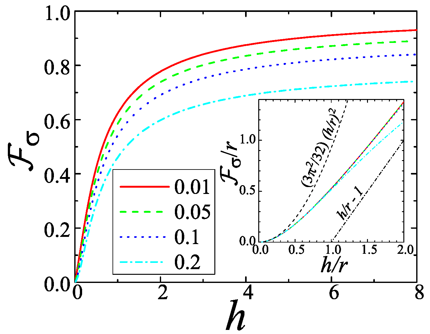
Figure 4: The dependence of the function $\mathcal{F}_{\sigma}(h,r)$ defined by Eqs. (43) and (44) on the reduced field $h$ for different values of $r$ specified in the legend. The inset shows the scaling plot of $\mathcal{F}_{\sigma}/r$ vs $h/r$ describing the crossover between the quadratic and linear regimes at small fields. The dashed and dot-dashed lines show the low-field quadratic and linear asymptotics.

Figure 5: The distribution functions $\Lambda_{s,x}(p_{s})$, Eq. (27), normalized to $v_{1,\alpha}^{\mathrm{hs}}\tau_{1}$ near the hot spot for different magnetic fields and representative parameters shown in the $h=0.1$ plot. For not too large fields, $h<1$, due to strong equilibration near hot spot, $\Lambda_{s,x}$ for two bands are very close at $p_{s}=0$. At zero magnetic field the distribution functions have symmetric dips with width $\sim p_{\tau,s}$. At fields $h>r_{s}$ the hot spot strongly disturbs the distribution function within the range $\Delta_{H}p_{s}\propto H$ on one side ($p_{1}>0$ for the electron band and $p_{2}<0$ for the hole band). As a consequence, the dependences $\Lambda_{s,x}(p_{s})$ have steps at $p_{s}=0$. The height of this step reduces with increasing field for $h>1$.

Calculation of the conductivity is based on the distribution functions $\Lambda_{s,x}(p_{s})$ defined by Eq. (27). Figure 5 illustrates how these functions evolve with increasing magnetic field. We can see that at zero field the functions have symmetric dips with width $p_{\tau,s}$, within which they approach almost identical values at the hot spot, as described in Sec. V. We also note that the hole distribution function changes sign near the hot spot meaning that the partial current due to the quasiparticles in this region flows in the direction opposite to the average transport current. This corresponds to the effect of negative transport times caused by strong interband scattering, as pointed out in Ref. Breitkreiz et al. (2013). At fields $h>r_{s}$ the distribution functions become strongly asymmetric. They are strongly suppressed at the side from which the hot spot can be reached during the orbital motion in the magnetic field, i.e., at $p_{1}>0$( $p_{2}<0$) for the electron (hole) band, see Eq. (34). The range of this suppression $\Delta_{H}p_{s}$ grows proportionally to the magnetic field. Due to such one-side suppression, the distribution functions acquire a steplike features at the hot spot. This sharp drop reflects small probability of quasiparticle penetration through the hot spot without scattering. This probability increases with increasing magnetic field and this corresponds to the step-height decrease.

Using the distribution functions from Eq. (27), we derive from Eq. (18b) the magnetic-field dependent part of $S_{\alpha\alpha}(H)$ as

$$\delta S_{\alpha\alpha}^{\mathrm{hs}}(H)\!=\!-\sum_{s}v_{s,\alpha}^{\mathrm{hs}}\left(v_{s,\alpha}^{\mathrm{hs}}\tau_{s}\!-\!\bar{\Lambda}_{\bar{s},\alpha}\right)\tau_{s}\gamma_{\mathrm{hs}}\mathcal{F}_{\sigma}(h,r_{s}).$$

In Eq. (18b) we again replaced $v_{s,\alpha}$ by its value at the hot spot $v_{s,\alpha}^{\mathrm{hs}}$. Substituting $\bar{\Lambda}_{\bar{s},\alpha}$ from Eq. (30), we obtain the field-dependent part of $S_{\alpha\alpha}$ in the closed form,

$$\delta S_{\alpha\alpha}^{\mathrm{hs}}(H) =-\gamma_{\mathrm{hs}}\left(v_{1,\alpha}^{\mathrm{hs}}\tau_{1}-\!v_{2,\alpha}^{\mathrm{hs}}\tau_{2}\right)$$

$$\times \frac{v_{1,\alpha}^{\mathrm{hs}}\tau_{1}R_{2}\mathcal{F}_{\sigma,1}-v_{2,\alpha}^{\mathrm{hs}}\tau_{2}R_{1}\mathcal{F}_{\sigma,2}}{R_{1}+R_{2}-R_{1}R_{2}},$$ (45)

where we used abbreviation $\mathcal{F}_{\sigma,s}\equiv\mathcal{F}_{\sigma}(h,r_{s})$. This equation determines the field-dependent part of longitudinal conductivity and represents the main result of this section. At high fields, $H\gg B_{w,s}$ ($h\gg r_{s}$), this general formula reproduces Eq. (35). In the linear regime for $B_{w,s}\ll H\ll B_{\gamma}$, we can derive somewhat more accurate result, which takes into account a finite offset,

$$\delta S_{\alpha\alpha}^{\mathrm{hs}}(H)\approx-\frac{1}{2}\left(\tau_{1}v_{1,\alpha}-\!\tau_{2}v_{2,\alpha}\right)^{2}\frac{e}{c}H+S_{\mathrm{off}}$$

with $S_{\mathrm{off}}=\frac{\gamma_{\mathrm{hs}}}{2}\left(\tau_{1}v_{1,\alpha}-\!\tau_{2}v_{2,\alpha}\right)\left(\tau_{1}v_{1,\alpha}r_{1}-\tau_{2}v_{2,\alpha}r_{2}\right)$. Note that this offset has the same order as the zero-field correction, see Eq. (25c). At small fields, $H\ll B_{w,s}$, we obtain

$$\delta S_{\alpha\alpha}^{\mathrm{hs}}(H) \approx-\frac{3\pi^{3/2}}{32}\frac{v_{1,\alpha}^{\mathrm{hs}}\tau_{1}-\!v_{2,\alpha}^{\mathrm{hs}}\tau_{2}}{\sqrt{\gamma_{\mathrm{hs}}}}$$

$$\times \frac{v_{1,\alpha}^{\mathrm{hs}}|v_{1}^{\mathrm{hs}}|\tau_{1}^{2}/w_{1}-v_{2,\alpha}^{\mathrm{hs}}|v_{2}^{\mathrm{hs}}|\tau_{2}^{2}/w_{2}}{\sqrt{|v_{2}^{\mathrm{hs}}|\tau_{2}/w_{2}}+\sqrt{|v_{1}^{\mathrm{hs}}|\tau_{1}/w_{1}}}\left(\frac{e}{c}H\right)^{2}.$$

For comparison, the conventional background contributionZiman (1960); Blatt (1968) is given by

$$\delta S_{s,\alpha\alpha}^{(0)}(H)\approx-\tau_{s}^{3}\int\left(v_{s,\alpha}^{\prime}\right)^{2}v_{s}dp_{s}\left(\frac{e}{c}H\right)^{2}$$ (46)

with $v_{s,\alpha}^{\prime}=dv_{s,\alpha}/dp_{s}$. We can see that, in contrast to the zero-field conductivity, the small-field $H^{2}$-correction is dominated by the hot-spot contribution. It exceeds the background correction by the factor $\sim p_{F,s}/p_{\tau,s}$.

Equations (42), (44), and (45) determine the hot-line contribution to the magnetoconductivity, Eq. (18a), for arbitrary values of band Fermi velocities, background scattering rates, and strength of hot-spot scattering. The qualitative behavior, however, is always the same: quadratic dependence at very small fields, linear magnetoconductivity in the intermediate field range, and approaching a constant value at very high fields. Such behavior was first predicted by Rosch Rosch (2000) for a single-band three-dimensional metal near the antiferromagnetic quantum critical point.

VI.2 Hall conductivity

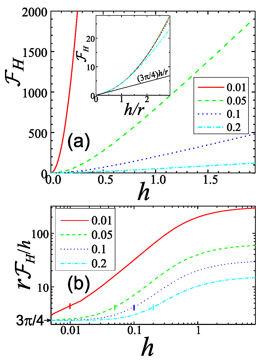
Figure 6: (a) Plots of the function $\mathcal{F}_{H}(h,r)$ defined by Eqs. (51) and (52) versus the reduced field $h$ for different values of $r$ specified in the legend. The inset shows the plot of $\mathcal{F}_{H}$ vs $h/r$ describing the crossover between the linear and quadratic regimes at small fields. (b) Double-logarithmic plots of $r\mathcal{F}_{H}(h,r)/h$ for the same parameters. The vertical bars mark the values $h=r$ at each plot. These plots clearly illustrate two crossovers in $\mathcal{F}_{H}(h,r)$ at $h\sim r$ and $h\sim 1$.

A finite contribution to the Hall conductivity appears due to the curvature of the Fermi surface at the hot spot. This means that the dependence of $v_{s,\alpha}^{\backprime}$ on $p_{s}^{\backprime}$ in Eqs. (27) and (29b) can not be neglected. It is sufficient to keep only the linear-expansion term, $v_{s,\alpha}(p_{s})\approx v_{s,\alpha}^{\mathrm{hs}}+v_{s,\alpha}^{\prime}p_{s}$ with $v_{s,\alpha}^{\prime}=dv_{s,\alpha}/dp_{s}$ at $p_{s}=0$. In this approximation the parameter $\mathcal{V}_{s,\alpha}$, Eq. (29b), can be represented as

$$\mathcal{V}_{s,\alpha}\approx v_{s,\alpha}^{\mathrm{hs}}R_{s}+v_{s,\alpha}^{\prime}\mathcal{B}_{s}$$ (47)

with

$$\mathcal{B}_{s}=\!\frac{1}{\tau_{s}\gamma_{\mathrm{hs}}}\int\limits_{-\infty}^{\infty}p_{s}^{\backprime}\frac{dp_{s}^{\backprime}}{|v_{s}^{\backprime}|}\!\int\limits_{-\delta_{s}\infty}^{p_{s}^{\backprime}}\!\frac{dp_{s}}{\frac{e}{c}H\tau_{s}v_{s}}\mathcal{M}_{H,s}(p_{s}^{\backprime},p_{s}),$$ (48)

where $\mathcal{M}_{H,s}(p_{s}^{\backprime},p_{s})$ is defined by Eq. (29c). The field dependence of this function determines behavior of the Hall conductivity which also has three regimes defined by the field scales $B_{w,s}$, Eq. (31), and $B_{\gamma}$, Eq. (33). For $H>B_{w,s}$ we can again approximate $\psi_{s}(p_{s})$ by $\delta$-function and this yields the following result

$$\mathcal{B}_{s}\approx\frac{1-\exp\left(-B_{\gamma}/H\right)}{\gamma_{\mathrm{hs}}}\left(\frac{e}{c}H\right)^{2}\tau_{s}v_{s}^{\mathrm{hs}},$$ (49)

meaning that $\mathcal{B}_{s}(H)$ increases quadratically with magnetic field in the range $B_{w,s}<H<B_{\gamma}$ and continues to grow linearly for $H>B_{\gamma}$. For smaller fields, $H<B_{w,s}$, the dependence $\mathcal{B}_{s}(H)$ is sensitive to exact shape of $\psi_{s}(p_{s})$, which we again assume to be Lorentzian, Eq. (38). In this case, using Eq. (41), we can derive the following scaling presentation for $\mathcal{B}_{s}(H)$,

$$\mathcal{B}_{s}=\delta_{s}w_{s}\mathcal{F}_{H}(H/B_{\gamma},r_{s}),$$ (50)

where the reduced function $\mathcal{F}_{H}(h,r)$ is defined by the following double integral,

$$\mathcal{F}_{H}(h,r)=\frac{r^{2}}{\pi}\int_{0}^{\infty}\!duu\int_{0}^{\infty}dz\exp\left(-z\right)$$

$$\times\left\{\exp\left[-\frac{\arctan\left(u\!+\!\pi hz/r^{2}\right)\!-\!\arctan u}{\pi h}\right]\right.$$

$$-\left.\exp\left[-\frac{\arctan u\!-\!\arctan\left(u\!-\!\pi hz/r^{2}\right)}{\pi h}\right]\right\},$$ (51)

and has the following asymptotics

$$\mathcal{F}_{H}(h,r)\approx\genfrac{\{}{.}{0.0pt}{}{\frac{3}{4}\pi\frac{h}{r}\left(1+\frac{5\pi^{3}}{32}\frac{h^{3}}{r^{3}}\right)\text{ for }h\ll r}{\pi\frac{h^{2}}{r^{2}}\left[1-\exp\left(-\frac{1}{h}\right)\right]\text{ for }h\gg r}.$$

In particular, the last asymptotics reproduces Eq. (49). In the case $r\ll 1$ we also derive in the appendix B a useful presentation containing only one integration,

$$\mathcal{F}_{H}(h,r) =\frac{h}{r}\int_{0}^{\infty}dxx\exp\left(-x\right)G_{H}\left(\frac{\pi hx}{4r}\right)$$

$$+\pi\frac{h^{2}}{r^{2}}\left[1-\exp\left(-\frac{1}{h}\right)\right]$$ (52)

with

$$G_{H}(a)\!=\!2\sqrt{a^{2}\!+\!1}E\!\left(\frac{a^{2}}{a^{2}\!+\!1}\right)\!-\!\frac{1}{2\sqrt{a^{2}\!+\!1}}K\!\left(\frac{a^{2}}{a^{2}\!+\!1}\right)\!-\!2a.$$

Plots of the function $\mathcal{F}_{H}(h,r)$ for different $r$ are shown in Fig. 6(a). For clearer illustration of the crossover between linear and quadratic regimes at small fields, the inset shows plot of $\mathcal{F}_{H}$ vs $h/r$ for $h<3r$. To demonstrate both crossovers at $h\sim r$ and $h\sim 1$, we show in Fig. 6(b) the double-logarithmic plot of $r\mathcal{F}_{H}(h,r)/h$.

We now proceed with derivation of the Hall conductivity. With corrections to $\mathcal{V}_{s,\alpha}$ given by Eqs. (47) and (50), the solution for $\bar{\Lambda}_{s,\alpha}$, Eq. (30), becomes

$$\bar{\Lambda}_{s,\alpha}=\sum_{l=s,\bar{s}}\left(U_{s,l}v_{l,\alpha}\tau_{l}+W_{s,l}\delta_{l}w_{l}v^{\prime}_{l,\alpha}\tau_{l}\right)$$ (53)

with

$$U_{s,s} =\frac{R_{s}}{R_{1}\!+\!R_{2}\!-\!R_{1}R_{2}},\ U_{s,\bar{s}}=\frac{R_{\bar{s}}\left(1-R_{s}\right)}{R_{1}\!+\!R_{2}\!-\!R_{1}R_{2}},$$

$$W_{s,s} =\frac{\mathcal{F}_{H,s}}{R_{1}\!+\!R_{2}\!-\!R_{1}R_{2}},\ W_{s,\bar{s}}=\frac{\mathcal{F}_{H,\bar{s}}\left(1-R_{s}\right)}{R_{1}\!+\!R_{2}\!-\!R_{1}R_{2}},$$

where we introduced abbreviations $\mathcal{F}_{H,s}\equiv\mathcal{F}_{H}(H/B_{\gamma},r_{s})$. From Eqs. (18b) and (27) we find that the Hall conductivity is determined by $S_{xy}=\sum_{s}S_{s,xy}$ with

$$S_{s,xy} \approx\int\frac{dp_{s}}{|v_{s}|}v_{s,x}$$

$$\times \left(\bar{\Lambda}_{\bar{s},y}+\int\limits_{p_{s}}^{\delta_{s}\infty}\!dp_{s}^{\backprime}\frac{\tau_{s}v_{s,y}^{\backprime}\!-\!\bar{\Lambda}_{\bar{s},y}}{\frac{e}{c}Hv_{s}^{\backprime}\tau_{s}}\mathcal{L}_{H,s}(p_{s}^{\backprime},p_{s})\right),$$ (54)

where $\mathcal{L}_{H,s}(p_{s}^{\backprime},p_{s})$ is defined by Eq. (26b) and for the Lorentzian hot spot can be estimated as

$$\mathcal{L}_{H,s}(p_{s}^{\backprime},p_{s}) \approx\exp\left[-\frac{p_{s}^{\backprime}\!-\!p_{s}}{\frac{e}{c}Hv_{s}\tau_{s}}\right.$$

$$-\left.\frac{\gamma_{\mathrm{hs}}}{\frac{e}{c}\pi H}\left(\arctan\frac{p_{s}^{\backprime}}{w_{s}}\!-\!\arctan\frac{p_{s}}{w_{s}}\right)\right].$$ (55)

First, we separate from $S_{s,xy}$ a conventional background contribution,

$$S_{s,xy}^{(0)} =\int\frac{dp_{s}}{|v_{s}|}v_{s,x}\int\limits_{p_{s}}^{\delta_{s}\infty}\ \frac{dp_{s}^{\backprime}}{v_{s}^{\backprime}}\frac{v_{s,y}^{\backprime}}{\frac{e}{c}H}\exp\left[-\frac{p_{s}^{\backprime}-p_{s}}{\frac{e}{c}Hv_{s}\tau_{s}}\right]$$

$$=-\delta_{s}\frac{e}{c}H\tau_{s}^{2}\int dp_{s}v_{s,x}v_{s,y}^{\prime}.$$ (56)

Subtracting this term, we obtain the hot-spot contribution, $S_{s,xy}^{\mathrm{hs}}=S_{s,xy}-S_{s,xy}^{(0)}$, as

$$S_{s,xy}^{\mathrm{hs}}\!\approx\!\int\frac{dp_{s}}{|v_{s}|}v_{s,x}\!\int\limits_{p_{s}}^{\delta_{s}\infty}\!\frac{dp_{s}^{\backprime}}{\frac{e}{c}Hv_{s}^{\backprime}\tau_{s}}\left(\bar{\Lambda}_{\bar{s},y}\!-\!\tau_{s}v_{s,y}^{\backprime}\right)\mathcal{M}_{H,s}(p_{s}^{\backprime},p_{s}),$$ (57)

where $\mathcal{M}_{H,s}(p_{s}^{\backprime},p_{s})$ is defined by Eq. (41). Substituting $\bar{\Lambda}_{s,\alpha}$ from Eq. (53) and expanding $v_{s,y}$ and $v_{s,x}^{\backprime}$ near the hot spot, after some algebraic transformations, we finally find the total hot-spot Hall term

$$S_{xy}^{\mathrm{hs}} =-\frac{\gamma_{\mathrm{hs}}}{R_{1}+R_{2}-R_{1}R_{2}}\sum_{s}\delta_{s}w_{s}\mathcal{F}_{H,s}R_{\bar{s}}\mathcal{K}_{s},$$ (58)

$$\mathcal{K}_{s} =\tau_{s}\left(\tau_{s}\left[\mathbf{v}_{s}^{\mathrm{hs}}\times\mathbf{v}_{s}^{\prime}\right]_{z}\!+\!\tau_{\bar{s}}\left[\mathbf{v}_{s}^{\prime}\times\mathbf{v}_{\bar{s}}^{\mathrm{hs}}\right]_{z}\right),$$

which determines the Hall conductivity via Eq. (18a). We can see that, in general, $S_{xy}^{\mathrm{hs}}$ contains both intraband and interband contributions.

As follows from Eq. (58), the hot-spot Hall conductivity has three asymptotic regimes: (i) Small-field linear regime, $h\ll r_{s}$,

$$S_{xy}^{\mathrm{hs}} \approx-\frac{3}{4}\pi\frac{\gamma_{\mathrm{hs}}h}{r_{1}+r_{2}}\sum_{s}\delta_{s}w_{s}\frac{r_{\bar{s}}}{r_{s}}\mathcal{K}_{s}$$

$$=\frac{3}{4}\frac{\frac{e}{c}H\sqrt{\pi\gamma_{\mathrm{hs}}}}{\sqrt{|v_{1}^{\mathrm{hs}}|\tau_{1}/w_{1}}+\sqrt{|v_{2}^{\mathrm{hs}}|\tau_{2}/w_{2}}}\sum_{s}v_{s}^{\mathrm{hs}}\tau_{s}\mathcal{K}_{s},$$ (59)

(ii) Intermediate quadratic regime, $r_{s}\ll h\ll 1$,

$$S_{xy}^{\mathrm{hs}} \approx-\frac{\pi}{2}\gamma_{\mathrm{hs}}h^{2}\sum_{s}\frac{\delta_{s}w_{s}}{r_{s}^{2}}\mathcal{K}_{s}$$

$$=-\frac{1}{2}\left(\frac{e}{c}H\right)^{2}\sum_{s}v_{s}^{\mathrm{hs}}\tau_{s}\mathcal{K}_{s},$$ (60)

and (iii) Large-field linear regime, $h>1$,

$$S_{xy}^{\mathrm{hs}} \approx-\pi\gamma_{\mathrm{hs}}h\sum_{s}\frac{\delta_{s}w_{s}}{r_{s}^{2}}\mathcal{K}_{s}$$

$$=\gamma_{\mathrm{hs}}\frac{e}{c}H\sum_{s}v_{s}^{\mathrm{hs}}\tau_{s}\mathcal{K}_{s}.$$ (61)

The latter two asympotics correspond to Eq. (49). Note that in all three asymptotics $S_{xy}^{\mathrm{hs}}$ is proportional to $\sum_{s}v_{s}^{\mathrm{hs}}\tau_{s}\mathcal{K}_{s}$ even though the general result, Eq. (58), does not have this property. Comparing $S_{xy}^{\mathrm{hs}}$, Eq. (58), and its asymptotics with the conventional contribution $S_{xy}^{(0)}$, Eq. (56), we can make several observations. The signs of the hot-spot correction terms are opposite to the corresponding conventional contributions. The correction to the linear Hall conductivity at $H<B_{w,s}$ is typically small. The relative correction is of the order of $p_{\tau}/p_{F}$, similar to the zero-field conductivity. However, the hot-spot correction leads to crossover to quadratic regime at relatively small magnetic fields, $H\sim B_{w,s}$, and this quadratic field dependence persists within a wide range of the magnetic fields. In combination with the linear decrease of the longitudinal conductivity, this behavior provides clear signatures of the hot-spot scattering. Comparing Eqs. (56) and (61), we can see that the overall relative change of slope of the partial Hall conductivity for bands $s$, $\sigma_{xy,s}$, from very small to very large field is determined by the hot-spot strength as

$$\frac{\Delta\sigma_{xy,s}^{\prime}}{\sigma_{xy,s}^{\prime}}\sim\frac{\gamma_{\mathrm{hs}}|v_{s}|\tau_{s}}{p_{F,s}}$$

with $\sigma_{xy,s}^{\prime}=\partial\sigma_{xy,s}/\partial H$ and $\Delta\sigma_{xy,s}^{\prime}=\sigma_{xy,s}^{\prime}(H\gg B_{\gamma})-\sigma_{xy,s}^{\prime}(H\rightarrow 0)$.

VII Representative magnetic field dependences for a simple four-band model

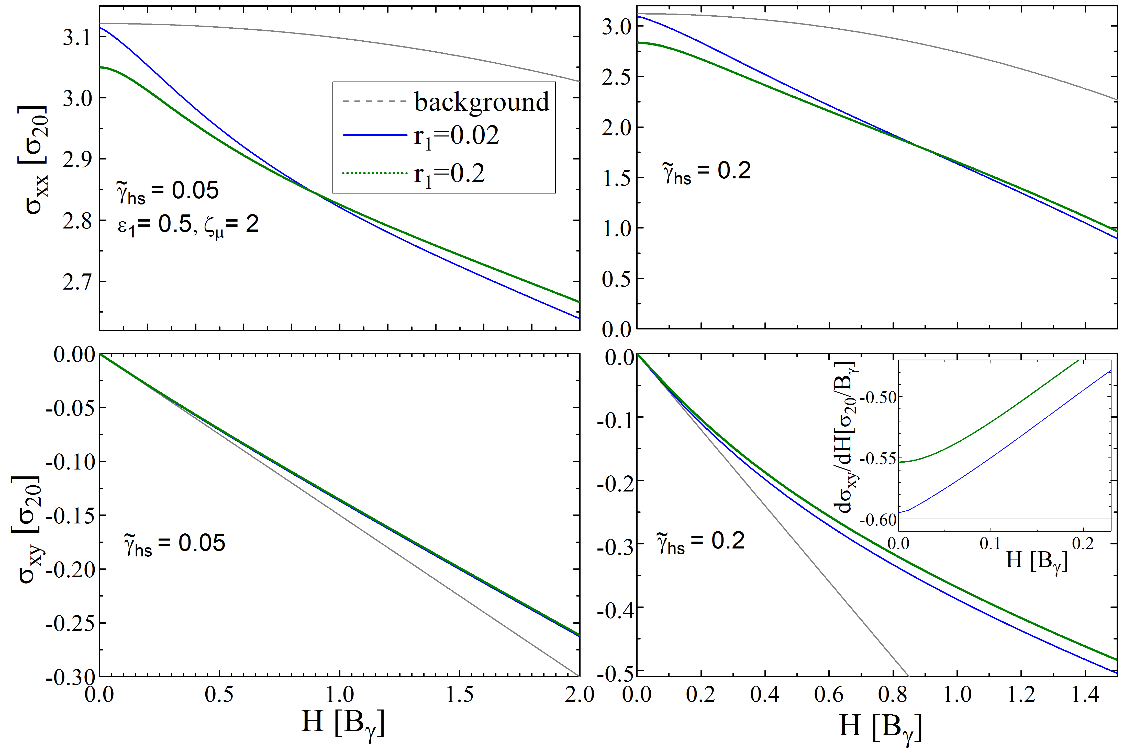
Figure 7: Representative magnetic field dependences of the conductivity components for two values of hot-spot strength $\tilde{\gamma}_{\mathrm{hs}}$, $0.05$ (left column) and $0.2$ (right column) and two values of “sharpness” parameter $r_{1}$, $0.02$ and $0.2$ (solid and dotted lines). For reference, we also show background conductivity without hot-spot scattering (dashed lines). The inset in the lower right plot show the derivative $d\sigma_{xy}/dH$ at low fields to emphasize the difference between two values of $r_{1}$.

In this section we illustrate general trends in the magnetic-field dependences of the conductivity components for different parameters. The iron pnictides and chalcogenides typically have at least two hole bands in the Brillouin zone center and two electron bands at the zone edge. This makes fully realistic analysis rather complicated and requires knowledge of many band-structure and scattering parameters. For illustration, we consider a minimum model of compensated metal with two identical hole and two electron Fermi surfaces. We assume circular and elliptical cross sections for the hole and electron Fermi surfaces respectively,

$$\xi_{1,\mathbf{p}}=\varepsilon_{1,0}-\mu+\frac{p_{x}^{2}}{2m_{x}}+\frac{p_{y}^{2}}{2m_{y}},\ \xi_{2,\mathbf{p}}=\varepsilon_{2,0}-\mu-\frac{p^{2}}{2m_{2}},$$

which are characterized by the Fermi momenta, $p_{F,2}=\sqrt{2m_{2}\varepsilon_{F,2}}$ and $p_{F,\alpha}=\sqrt{2m_{\alpha}\varepsilon_{F,1}}$ with $\alpha=x,y$, $\varepsilon_{F,1}=\mu-\varepsilon_{1,0}$, $\varepsilon_{F,2}=\varepsilon_{2,0}-\mu$. In the further analysis, we will assume that the inequality $p_{F,x}>p_{F,2}>p_{F,y}$ holds. The second electron band is 90^∘-rotated with respect to the first one. Each electron band has four hot spots and each hole band has eight hot spots. Introducing the ratios, $u_{\alpha}=p_{F,2}/p_{F,\alpha}$ with $u_{x}<1$ and $u_{y}>1$, we find the cosine and sine of the hot-spot angle $\theta_{\mathrm{hs}}$ as

$$\cos^{2}\theta_{\mathrm{hs}}=\frac{u_{y}^{2}-1}{u_{y}^{2}-u_{x}^{2}},\ \sin^{2}\theta_{\mathrm{hs}}=\frac{1-u_{x}^{2}}{u_{y}^{2}-u_{x}^{2}}.$$ (62)

For the compensated case $u_{x}u_{y}=1$.

In the previous sections we focused on a single $p_{z}$ cross section of the Fermi surface. Calculation of the conductivity in Eq. (18a) includes the integration over $p_{z}$, which means averaging over all cross sections. For estimate, we will use result for a single representative cross section. As the conductivity unit, we take the partial conductivity of the hole bands at zero magnetic field, $\sigma_{20}\equiv\sigma_{2,xx}(0)\propto S_{2,xx}^{(0)}(0)$. We also introduce notations for the in-plane mass anisotropy of the electron band $\epsilon_{1}=m_{y}/m_{x}$, the average mobility ratio $\zeta_{\mu}=m_{2}\tau_{1}/\bar{m}\tau_{2}$ with $\bar{m}=\sqrt{m_{x}m_{y}}$, and the reduced hot-spot strength

$$\tilde{\gamma}_{\mathrm{hs}}=\gamma_{\mathrm{hs}}|v_{2}|\tau_{2}/p_{F,2}\ll 1.$$

In these notations the ratios of the mobility components are $\tau_{1}v_{F,x}/\tau_{2}|v_{2}|=\xi_{\mu}/u_{y}$, $\tau_{1}v_{F,y}/\tau_{2}|v_{2}|=\xi_{\mu}/u_{x}$.

Using the reduced parameters, we obtain the following presentations for the background zero-field conductivity

$$\sigma_{xx}^{(0)}(0)=\sigma_{20}\left[1+\zeta_{\mu}\left(u_{x}^{-2}+u_{y}^{-2}\right)/2\right],$$

magnetoconductivity

$$\delta\sigma_{xx}^{(0)}(h)=-\sigma_{20}\tilde{\gamma}_{\mathrm{hs}}^{2}h^{2}\left[1+\left(u_{x}^{-2}+u_{y}^{-2}\right)\zeta_{\mu}^{3}/2\right],$$

and Hall conductivity

$$\sigma_{xy}^{(0)}=\sigma_{20}\tilde{\gamma}_{\mathrm{hs}}h\left(1-\frac{\zeta_{\mu}^{2}}{u_{x}u_{y}}\right).$$

Note that the parameter $\tilde{\gamma}_{\mathrm{hs}}$ appears in these presentation only because we use the field scale $B_{\gamma}$ which is proportional to $\gamma_{\mathrm{hs}}$.

The contributions from the four hot spots are determined by the ratios of the local mobilities at these points which can be evaluated as $\tau_{1}v_{1,x}^{\mathrm{hs}}/\tau_{2}|v_{2,x}^{\mathrm{hs}}|\!=\!\xi_{\mu}\sqrt{\epsilon_{1}}$ and $\tau_{1}v_{1,y}^{\mathrm{hs}}/\tau_{2}|v_{2,y}^{\mathrm{hs}}|$ $=\!\xi_{\mu}/\sqrt{\epsilon_{1}}$. We also obtain relation between the parameters $r_{s}$, Eq. (40), $r_{2}^{2}=r_{1}^{2}\frac{w_{2}}{w_{1}}\zeta_{\mu}\sqrt{u_{x}^{-2}+u_{y}^{-2}-1}$ and assume that $w_{1}=w_{2}$. The hot-spot contributions to the zero-field conductivity, Eq. (25c) and longitudinal magnetoconductivity, Eq. (45), can now be presented as

$$\sigma_{xx}^{\mathrm{hs}}(0)=-\frac{4}{\pi}\frac{\sigma_{20}\tilde{\gamma}_{\mathrm{hs}}}{1/r_{1}+1/r_{2}}$$

$$\times\!\left[\cos^{2}\theta_{\mathrm{hs}}\left(1\!+\zeta_{\mu}\sqrt{\epsilon_{1}}\right)^{2}\!+\sin^{2}\theta_{\mathrm{hs}}\left(1\!+\zeta_{\mu}/\sqrt{\epsilon_{1}}\right)^{2}\right],$$ (63)

and

$$\delta\sigma_{xx}^{\mathrm{hs}}(H)=-\frac{4}{\pi}\frac{\sigma_{20}\tilde{\gamma}_{\mathrm{hs}}}{R_{1}+R_{2}-R_{1}R_{2}}$$

$$\times\Big{[}\cos^{2}\theta_{\mathrm{hs}}\left(\zeta_{\mu}\sqrt{\epsilon_{1}}+\!1\right)\left(\zeta_{\mu}\sqrt{\epsilon_{1}}R_{2}\mathcal{F}_{\sigma,1}+R_{1}\mathcal{F}_{\sigma,2}\right)$$

$$+\sin^{2}\theta_{\mathrm{hs}}\left(\frac{\zeta_{\mu}}{\sqrt{\epsilon_{1}}}+\!1\right)\left(\frac{\zeta_{\mu}}{\sqrt{\epsilon_{1}}}R_{2}\mathcal{F}_{\sigma,1}+R_{1}\mathcal{F}_{\sigma,2}\right)\Big{]},$$ (64)

respectively. For the derivation of the Hall term, Eq. (58), we obtain the following relations

$$\frac{\tau_{1}\left[\mathbf{v}_{1}^{\mathrm{hs}}\times\mathbf{v}_{1}^{\prime}\right]_{z}}{\tau_{2}\left[\mathbf{v}_{1}^{\prime}\times\mathbf{v}_{2}^{\mathrm{hs}}\right]_{z}}=\frac{\tau_{1}\left[\mathbf{v}_{2}^{\prime}\times\mathbf{v}_{1}^{\mathrm{hs}}\right]_{z}}{\tau_{2}\left[\mathbf{v}_{2}^{\mathrm{hs}}\times\mathbf{v}_{2}^{\prime}\right]_{z}}=\frac{\tau_{1}\varepsilon_{F,1}}{\tau_{2}\varepsilon_{F,2}}=\frac{\xi_{\mu}}{u_{x}u_{y}},$$

which allow us to present this term as

$$\sigma_{xy}^{\mathrm{hs}}(H)\!=\!\frac{8}{\pi^{2}}\sigma_{20}\tilde{\gamma}_{\mathrm{hs}}^{2}\frac{r_{1}^{2}\zeta_{\mu}^{2}\mathcal{F}_{H,1}R_{2}\!-\!r_{2}^{2}\mathcal{F}_{H,2}R_{1}}{R_{1}+R_{2}-R_{1}R_{2}}\left(1\!+\!\frac{\zeta_{\mu}}{u_{x}u_{y}}\right).$$ (65)

We utilize the derived presentations for illustration of the possibles shapes of $\sigma_{\alpha\beta}(H)$ dependences.

The overall behavior of the conductivity components mostly depends on the two reduced parameters $\tilde{\gamma}_{\mathrm{hs}}$ and $r_{1}$. The first parameter determines the magnitude of the hot-spot correction with respect to background while the second parameter determines the behavior at small magnetic fields. Figure 7 shows the representative magnetic-field dependences of the conductivity components for two values of $\tilde{\gamma}_{\mathrm{hs}}$, $0.05$ and $0.2$ and two values of $r_{1}$, $0.02$ and $0.2$. As a reference, we also show the background longitudinal and Hall conductivities without hot-spot scattering.

We can see that for the weak hot spot, $\tilde{\gamma}_{\mathrm{hs}}=0.05$, the corrections are small while for $\tilde{\gamma}_{\mathrm{hs}}=0.2$ they become comparable with the background. In particular, the slope of the Hall conductivity $|d\sigma_{xy}/dH|$ drops more than twice with increasing magnetic field. The role of the “sharpness” parameter $r_{1}$ is more obvious for the longitudinal conductivity. For the broad hot spot, $r_{1}=0.2$, we can see the region of quadratic magnetoconductivy for $h<0.2$. For the narrow hot spot, $r_{1}=0.02$, this region is practically invisible in the plots and the conductivity has linear magnetic-field dependence in the extended field range. In contrast, for $r_{1}=0.2$ this linear regime is not pronounced and looks more like an inflection point. The parameter $r_{1}$ only weakly influences the shape of $\sigma_{xy}(H)$ because it mostly determines the small correction to the low-field linear slope. This small correction can be more clearly seen in the field dependence of the derivative $d\sigma_{xy}/dH$ at small fields, see the inset in the lower right plot of Fig. (7). Also, the inset plots clearly demonstrate that the hot-spot correction to $\sigma_{xy}$ has quadratic magnetic-field dependence in the intermediate field range.

VIII Summary and discussion

In summary, we analyzed in detail magnetotransport due to the hot-spot scattering on the AF fluctuations in multiple-band metals. The key qualitative features are extended ranges of the linear magnetic-field dependence of longitudinal conductivity and, simultaneously, the quadratic dependence of the Hall component.

This mechanism is very likely responsible for anomalous magnetotransport properties found in some iron pnictides and chalcogenides in paramagnetic state. For example, the linear magnetoresistance and strongly nonlinear Hall resistivity have been found in Fe_1+yTe_0.6Se_0.4Sun et al. (2014). This behavior becomes pronounced after annealing which strongly reduces background scattering. Such behavior roughly corresponds to illustration in Fig. 7 for strong and narrow hot spot, $\tilde{\gamma}_{\mathrm{hs}}\!=\!0.2$ and $r_{1}\!=\!0.02$ for $H<B_{\gamma}$. The absence of saturation at high magnetic fields simply means that the field scale $B_{\gamma}$ for this compound is very high, more than $30$ tesla. In other compound, Ba[As_1-xP_x]₂Fe₂, longitudinal resistance has small but clear deviations from quadratic magnetic-filed dependence Jia et al. ; Analytis et al. (2014) while the Hall resistance has weakly nonlinear field dependence Jia et al. . Such behavior resembles illustration in Fig. 7 for weak and broad hot-spot, $\tilde{\gamma}_{\mathrm{hs}}\!=\!0.05$ and $r_{1}\!=\!0.2$. The corresponding typical magnetic fields seem to be rather large, $B_{w}\sim 35$T and $B_{\gamma}\sim 65$T. Anomalous properties are seen in the optimally-doped compound and they disappear in overdoped compounds. This is consistent with the interpretation based on the spin-fluctuation scattering. In principle, detailed analysis of magnetotransport allows to extract the hot-spot parameters which would give us a valuable microscopic information about properties of spin fluctuations.

It is instructive to compare behavior of magnetotransport in the paramagnetic state due to hot-spot scattering and in the antiferromagnetic state due to Fermi surface reconstruction Fenton and Schofield (2005); Lin and Millis (2005); Koshelev (2013). In both cases the anomalous behavior is caused by the interruption of smooth orbital motion of quasiparticles along the Fermi surface in the magnetic field. In the first case the interruption is caused by the sharp enhancement of scattering and in the second case by the abrupt change of the Fermi velocity. In both cases there is a low-field crossover at which the field dependence of the longitudinal conductivity changes from quadratic to linear while the dependence of the Hall conductivity changes from linear to quadratic. For the hot-spot mechanism the crossover field is determined by the scattering strength and width of the hot spots and for the reconstruction mechanism it is determined be the antiferromagnetic gap. Above the crossover both the hot spots and turning points can be treated as sharp regions and the conductivity components are not sensitive to their internal structure. We can note that for identical background scattering times $\tau_{1}=\tau_{2}$ in the linear regime the longitudinal conductivity due to the hot-spots is two times smaller than one due to the reconstruction mechanism. For the hot-spot mechanism the linear (quadratic) growth of the longitudinal (Hall) conductivity is limited from above by the second magnetic field scale determined by the total scattering strength. Such limit is absent for the reconstruction mechanism.

Appendix A Function $\mathcal{F}_{\sigma}(h,r)$ for $r\ll 1$

In the case $r\ll 1$ the two crossovers in the behavior of the function $\mathcal{F}_{\sigma}(h,r)$ , Eq. (43), are well separated. This allows us to derive a useful presentation for this function containing only single integration. In the region $h\ll 1$ the ratio $\mathcal{F}_{\sigma}(h,r)/r$ depends on the single parameter $h/r$. Therefore, for the analysis of this region, it is convenient to introduce new function $F_{\sigma}(b,r)$ defined by the relation

$$\mathcal{F}_{\sigma}(h,r)=(r/\pi)F_{\sigma}(\pi h/r,r).$$ (66)

This new function is defined as

$$F_{\sigma}(b,r)=\int_{-\infty}^{\infty}dv\int_{0}^{\infty}dz\exp\left(-z\right)\left\{\exp\left[-\frac{z}{r^{2}+v^{2}}\right]-\exp\left[-\frac{\arctan\left(\left(v+\frac{bz}{2}\right)/r\right)-\arctan\left(\left(v-\frac{bz}{2}\right)/r\right)}{rb}\right]\right\},$$ (67)

where $b=\pi h/r$ is the redefined reduced field. For $r\ll 1,\pi/b$, using asympotics $\arctan x\approx\pm\pi/2\mp 1/x$ for $x\rightarrow\pm\infty$, we can approximate

$$\arctan\left(\frac{v+\frac{bz}{2}}{r}\right)-\arctan\left(\frac{v-\frac{bz}{2}}{r}\right)\approx\genfrac{\{}{.}{0.0pt}{}{\frac{rbz}{v^{2}-\frac{\left(bz\right)^{2}}{4}}\;\text{, for}\;|v|-\frac{bz}{2}\gg r}{\pi-\frac{2vr}{v^{2}-\frac{\left(bz\right)^{2}}{4}}\;\text{, for}\;\frac{bz}{2}-|v|\gg r}.$$

We can conclude that the region $|v|<\frac{bz}{2}$ gives very small contribution to the second-term integration in Eq. (67) because it contains exponentially small factor $\exp(-\pi/rb)$. Therefore, we can rewrite $F_{\sigma}(b,r)$ as

$$F_{\sigma}(b) =\int_{0}^{\infty}dz\exp\left(-z\right)\left[\int_{|v|>0}dv\exp\left(-\frac{z}{v^{2}}\right)\right.$$

$$-\left.\int_{|v|>\frac{bz}{2}}dv\exp\left(-\frac{z}{v^{2}-\frac{\left(bz\right)^{2}}{4}}\right)\right].$$

We can see that this function does not depend explicitly on the parameter $r$. It describes the crossover between the quadratic and linear regimes for $b\ll\pi/r$. Performing variable change $v\rightarrow v+bz/2$ in the second term, we obtain

$$\int_{0}^{v_{0}}dv\exp\left(-\frac{z}{v^{2}}\right)-\int_{\frac{bz}{2}}^{v_{0}}dv\exp\left(-\frac{z}{v^{2}-\frac{\left(bz\right)^{2}}{4}}\right)$$

$$=\int_{0}^{v_{0}}dv\exp\left(-\frac{z}{v^{2}}\right)-\int_{0}^{v_{0}-\frac{bz}{2}}dv\exp\left(-\frac{z}{v^{2}+bzv}\right)$$

$$=\int_{0}^{v_{0}}dv\left[\exp\left(-\frac{z}{v^{2}}\right)-\exp\left(-\frac{z}{v^{2}+bzv}\right)\right]+\frac{bz}{2},$$

where $v_{0}\gg 1$ is an arbitrary upper cut off which can be sent to infinity in the last formula. After these transformations, $F_{\sigma}(b)$ takes the following form

$$F_{\sigma}(b) =2\int\limits_{0}^{\infty}dz\int\limits_{0}^{\infty}dv\exp\left(-z\right)$$

$$\times \left[\exp\left(-\frac{z}{v^{2}}\right)-\exp\left(-\frac{z}{v^{2}+bzv}\right)\right]+b$$

$$=2 \int\limits_{0}^{\infty}dv\left[\frac{v^{2}}{v^{2}+1}-\int_{0}^{\infty}dz\exp\left(-z-\frac{z}{v^{2}+bzv}\right)\right]+b.$$

To eliminate a complicated expression in the exponent, we make the variable change

$$x=z+\frac{z}{v^{2}+bzv},$$

$$z =-\frac{\left(v^{2}+1-xbv\right)}{2vb}+\sqrt{\frac{\left(v^{2}+1-xbv\right)^{2}}{4v^{2}b^{2}}+\frac{xv}{b}},$$

which allows us to present $F_{\sigma}(b)$ as

$$F_{\sigma}(b)=\int_{0}^{\infty}dx\exp\left(-x\right)G\left(\frac{bx}{4}\right)-\pi$$ (68)

with

$$G(a)=\int_{0}^{\infty}dv\left(1-\frac{v^{2}-1+4av}{\sqrt{\left(v^{2}\!-1+4av\right)^{2}+4v^{2}}}\right)+4a.$$

Introducing a new variable $\zeta$ defined by $2\zeta=v-1/v+2a$ with the inverse relation $v=\left(\zeta-a\right)+\sqrt{\left(\zeta-a\right)^{2}+1}$, we obtain the presentation

$$G(a)=2\int_{0}^{\infty}d\zeta\left(1-\frac{\zeta^{2}-a^{2}}{\sqrt{\left(\zeta^{2}\!+\!a^{2}\!+\!1\right)^{2}\!-\!4a^{2}\zeta^{2}}}\right).$$ (69)

This integral can be transformed to the elliptic form by the substitution

$$s=\frac{2\sqrt{a^{2}+1}}{\zeta+\left(a^{2}+1\right)/\zeta}.$$

In this case the integration in Eq. (69) splits into two segments: (i) the interval of $\zeta$ between $0$ and $\zeta_{0}=\sqrt{a^{2}+1}$ corresponds to variation of $s$ from $0$ to $1$ with $\zeta=\frac{1}{s}\sqrt{a^{2}+1}\left(1-\sqrt{1-s^{2}}\right)$ and (ii) the interval of $\zeta$ between $\zeta_{0}$ and $\infty$ corresponds to variation of $s$ from $1$ to $0$ with $\zeta=\frac{1}{s}\sqrt{a^{2}+1}\left(1+\sqrt{1-s^{2}}\right)$. The substitution transforms $G(a)$ to the following form

$$G(a) =2\sqrt{a^{2}+1}\int\limits_{0}^{1}\frac{ds}{s^{2}}\sum_{\delta=\pm 1}\delta\left(1+\frac{\delta}{\sqrt{1-s^{2}}}\right)$$

$$\times \left(1-\frac{1-m_{a}+\delta\left(1+m_{a}\right)\sqrt{1-s^{2}}}{2\sqrt{1-m_{a}s^{2}}}\right)$$

$$=2 \sqrt{a^{2}\!+\!1}\int\limits_{0}^{1}\frac{ds}{\sqrt{1\!-\!s^{2}}}\left(2\frac{1\!-\!\sqrt{1\!-\!m_{a}s^{2}}}{s^{2}}+\frac{1-m_{a}}{\sqrt{1-m_{a}s^{2}}}\right)$$

with $m_{a}=\frac{a^{2}}{a^{2}+1}$. The first term in the parenthesis can be reduced to the full elliptic integrals,

$$K(m)\!=\!\int\limits_{0}^{1}\frac{dt}{\sqrt{1\!-\!t^{2}}\sqrt{1\!-\!mt^{2}}}\hbox{ and }E(m)\!=\!\int\limits_{0}^{1}\frac{\sqrt{1\!-\!mt^{2}}}{\sqrt{1-t^{2}}}dt,$$

using integration by parts

$$\int_{0}^{1}\frac{1-\sqrt{1-ms^{2}}}{s^{2}\sqrt{1-s^{2}}}ds=-\int_{0}^{1}\left(1-\sqrt{1-ms^{2}}\right)d\frac{\sqrt{1-s^{2}}}{s}$$

$$=m\int_{0}^{1}ds\frac{\sqrt{1-s^{2}}}{\sqrt{1-ms^{2}}}=-\left(1-m\right)K(m)+E(m).$$

This gives us final result

$$G(a)\!=\!4\sqrt{1\!+\!a^{2}}E\left(\frac{a^{2}}{1\!+\!a^{2}}\right)\!-\!\frac{2}{\sqrt{1\!+\!a^{2}}}K\left(\frac{a^{2}}{1\!+\!a^{2}}\right).$$ (70)

This result together with Eq. (68) describes behavior of $F_{\sigma}(b,r)$ for $b\ll\pi/r$. Namely, it describes a crossover between the low-field quadradic regime, $F(b)\approx(3\pi/32)b^{2}$ for $b\ll 1$ and the linear regime, $F(b)\approx b-\pi$ for $1\ll b\ll\pi/r$. To obtain presentation valid in the whole field range, one can simply add factor $1-\exp(-\pi/rb)$ to the integral term in Eq. (68)

$$F_{\sigma}(b,r)\!=\!\int\limits_{0}^{\infty}dx\exp\left(-x\right)G\left(\frac{bx}{4}\right)\left[1\!-\!\exp\left(-\frac{\pi}{rb}\right)\right]\!-\!\pi.$$ (71)

Transformation back to the function $\mathcal{F}_{\sigma}(h,r)$ using Eq. (66) gives Eq. (44) of the main text.

Appendix B Function $\mathcal{F}_{H}(h,r)$ at $r\ll 1$.

In this appendix we obtain a useful presentation of the function $\mathcal{F}_{H}(h,r)$ defined by Eq. (51) for $r\ll 1$ following the route similar to one in the Appendix A. First, we introduce the new reduced field $b=\pi h/r$ and make variable change $u=v/r$ giving the following presentation

$$\mathcal{F}_{H}(b,r)\! =\!\frac{1}{\pi}\int\limits_{0}^{\infty}dz\exp\left(-z\right)\int\limits_{0}^{\infty}\!dvv$$

$$\times \left\{\exp\left[-\frac{\arctan\left[\left(v\!+\!bz\right)/r\right]\!-\!\arctan\left(v/r\right)}{rb}\right]\right.$$

$$-\left.\!\!\exp\left[-\frac{\arctan\left(v/r\right)\!-\!\arctan\left[\left(v\!-\!bz\right)/r\right]}{rb}\right]\right\}.$$

In the case $r\ll 1,\pi/b$ we can use the asymptotics $\arctan x\approx\pm\pi/2\mp 1/x$ for $x\rightarrow\pm\infty$ in the most part of the integration domain . We note that the region $0<v<bz$ gives negligible contribution to the second-term integration because it contains exponentially small factor $\exp(-\pi/rb)$. Therefore, we can approximate $F_{H}(b,r)$ as

$$\mathcal{F}_{H}(b,r) \approx\frac{1}{\pi}\int\limits_{0}^{\infty}dz\exp\left(-z\right)\left[\int\limits_{0}^{\infty}vdv\exp\left(-\frac{z}{v\left(v\!+\!bz\right)}\right)\right.$$

$$-\left.\int\limits_{bz}^{\infty}vdv\exp\left(-\frac{z}{v\left(v-bz\right)}\right)\right].$$

We see that the dependence on $r$ droped out in this presentation. Shifting the integration in the second term, $v\rightarrow bz+v$, we derive the following presentation

$$\mathcal{F}_{H}(b)\approx\frac{b}{\pi}\int\limits_{0}^{\infty}dv\left[1\!-\!\int\limits_{0}^{\infty}dzz\exp\left(-z\!-\frac{z}{v\left(v\!+\!bz\right)}\right)\right]+\frac{b^{2}}{\pi}.$$

To remove complicated expression in the exponent, we make the variable change

$$x=z+\frac{z}{v^{2}+bzv},$$

$$z =\frac{xvb-v^{2}-1+\sqrt{\left(v^{2}-1+xbv\right)^{2}+4v^{2}}}{2vb},$$

which leads to the following presentation

$$\mathcal{F}_{H}(b)=\frac{b}{\pi}\int_{0}^{\infty}dxx\exp\left(-x\right)G_{H}\left(\frac{bx}{4}\right)+\frac{b^{2}}{\pi}$$ (72)

with

$$G_{H}(a) =\frac{1}{2}\int_{0}^{\infty}dv\left[1-\frac{\left(v^{2}-1+4av\right)}{\sqrt{\left(v^{2}-1+4av\right)^{2}+4v^{2}}}\right.$$

$$+\frac{2}{\sqrt{\left(v^{2}-1+4av\right)^{2}+4v^{2}}}$$

$$+\left.\frac{1}{4av}\left(1-\frac{\left(v^{2}+1+4av\right)}{\sqrt{\left(v^{2}-1+4av\right)^{2}+4v^{2}}}\right)\right],$$

To transform this function, we first introduce new variable $\zeta$ as

$$2\zeta=v-1/v+2a,$$

$$v =\left(\zeta-a\right)+\sqrt{\left(\zeta-a\right)^{2}+1},$$

leading to

$$G_{H}(a)\! =\int_{0}^{\infty}d\zeta\left(1-\frac{\zeta^{2}-a^{2}}{\sqrt{\left(\zeta^{2}+a^{2}+1\right)^{2}-4\zeta^{2}a^{2}}}\right.$$

$$+\left.\frac{1}{2\sqrt{\left(\zeta^{2}+a^{2}+1\right)^{2}-4\zeta^{2}a^{2}}}\right)-2a.$$

This integral reduces to the elliptic form with substitution

$$s =\frac{2\sqrt{a^{2}+1}}{\zeta+\frac{a^{2}+1}{\zeta}},$$

$$\zeta =\frac{\sqrt{a^{2}+1}}{s}\left(1\pm\sqrt{1-s^{2}}\right).$$

The $\zeta$ integrations splits into two domains

$$0 <\zeta<\zeta_{0}\rightarrow\zeta=\frac{1}{s}\sqrt{a^{2}+1}\left(1-\sqrt{1-s^{2}}\right),0<s<1$$

$$\zeta_{0} <\zeta<\infty\rightarrow\zeta=\frac{1}{s}\sqrt{a^{2}+1}\left(1+\sqrt{1-s^{2}}\right),1>s>0$$

with $\zeta_{0}=\sqrt{a^{2}+1}$ and integral for $G_{H}(a)$ becomes

$$G_{H}(a)=\sqrt{a^{2}+1}\int\limits_{0}^{1}\frac{ds}{s^{2}}\sum_{\delta=\pm 1}\delta\left(1+\frac{\delta}{\sqrt{1-s^{2}}}\right)$$

$$\times\left(1-\frac{1-m_{a}}{4\sqrt{1-m_{a}s^{2}}}-\delta\frac{\left(3+m_{a}\right)\sqrt{1-s^{2}}}{4\sqrt{1-m_{a}s^{2}}}\right)-2a$$

$$=\!2\sqrt{a^{2}\!+\!1}\!\int\limits_{0}^{1}\!\frac{ds}{s^{2}}\frac{4\sqrt{1\!-\!m_{a}s^{2}}\!-\!1\!+\!m_{a}-\left(3\!+\!m_{a}\right)\left(1\!-\!s^{2}\right)}{4\sqrt{1-s^{2}}\sqrt{1-m_{a}s^{2}}}$$

$$-2a$$

with $m_{a}=a^{2}/(a^{2}+1)$. This integral can be expressed via the full elliptic integrals $E(m)$ and $K(m)$ as

$$G_{H}(a)=2\sqrt{a^{2}\!+\!1}\left[E(m_{a})-\frac{1\!-\!m_{a}}{4}K(m_{a})\right]\!-\!2a.$$ (73)

Using asymptotics

$$G_{H}(a)\approx\frac{\ln\left(4a\right)+1}{2a}\text{ for }a\gg 1,$$

we obtain more accurate high-field asymptotics of $\mathcal{F}_{H}(b)$

$$\mathcal{F}_{H}(b)\approx\frac{b^{2}}{\pi}+\frac{2}{\pi}\left(\ln b-\gamma_{E}+1\right)\text{ for }b\gg 1.$$

Finally, to extend the presentation (72) to the whole range of fields including $b>\pi/r$, it is sufficient to add the factor $1-\exp(-1/h)=1-\exp(-\pi/br)$ to the last term, i.e.,

$$\mathcal{F}_{H}(b) \approx\frac{b}{\pi}\int_{0}^{\infty}dxx\exp\left(-x\right)G_{H}\left(\frac{bx}{4}\right)$$

$$+\frac{b^{2}}{\pi}\left[1-\exp\left(-\frac{\pi}{br}\right)\right].$$ (74)

Returning back to $h=rb/\pi$, we obtain Eq. (52) of the main text.

References

- Paglione and Greene (2010) J. Paglione and R. L. Greene, Nat. Phys. 6, 645 (2010).
- Stewart (2011) G. R. Stewart, Rev. Mod. Phys. 83, 1589 (2011).
- Shibauchi et al. (2014) T. Shibauchi, A. Carrington, and Y. Matsuda, Annu. Rev. Condens. Matter Phys. 5, 113 (2014).
- Hosono and Kuroki (2015) H. Hosono and K. Kuroki, Physica C 514, 399 (2015).
- Gooch et al. (2009) M. Gooch, B. Lv, B. Lorenz, A. M. Guloy, and C.-W. Chu, Phys. Rev. B 79, 104504 (2009).
- Kasahara et al. (2010) S. Kasahara, T. Shibauchi, K. Hashimoto, K. Ikada, S. Tonegawa, R. Okazaki, H. Shishido, H. Ikeda, H. Takeya, K. Hirata, T. Terashima, and Y. Matsuda, Phys. Rev. B 81, 184519 (2010).
- Hlubina and Rice (1995) R. Hlubina and T. M. Rice, Phys. Rev. B 51, 9253 (1995).
- Stojkovic and Pines (1997) B. P. Stojkovic and D. Pines, Phys. Rev. B 55, 8576 (1997).
- Löhneysen et al. (2007) H. v. Löhneysen, A. Rosch, M. Vojta, and P. Wölfle, Rev. Mod. Phys. 79, 1015 (2007).
- Kontani (2008) H. Kontani, Rep. Prog. Phys. 71, 026501 (2008).
- Fernandes et al. (2011) R. M. Fernandes, E. Abrahams, and J. Schmalian, Phys. Rev. Lett. 107, 217002 (2011).
- Breitkreiz et al. (2014a) M. Breitkreiz, P. M. R. Brydon, and C. Timm, Phys. Rev. B 89, 245106 (2014a).
- Breitkreiz et al. (2014b) M. Breitkreiz, P. M. R. Brydon, and C. Timm, Phys. Rev. B 90, 121104 (2014b).
- Blomberg et al. (2013) E. C. Blomberg, M. A. Tanatar, R. M. Fernandes, I. I. Mazin, B. Shen, H.-H. Wen, M. D. Johannes, J. Schmalian, and R. Prozorov, Nat. Commun. 4, 1914 (2013).
- Breitkreiz et al. (2013) M. Breitkreiz, P. M. R. Brydon, and C. Timm, Phys. Rev. B 88, 085103 (2013).
- Rosch (2000) A. Rosch, Phys. Rev. B 62, 4945 (2000).
- Rullier-Albenque et al. (2009) F. Rullier-Albenque, D. Colson, A. Forget, and H. Alloul, Phys. Rev. Lett. 103, 057001 (2009).
- Rullier-Albenque et al. (2010) F. Rullier-Albenque, D. Colson, A. Forget, P. Thuéry, and S. Poissonnet, Phys. Rev. B 81, 224503 (2010).
- Tsukada et al. (2010) I. Tsukada, M. Hanawa, S. Komiya, T. Akiike, R. Tanaka, Y. Imai, and A. Maeda, Phys. Rev. B 81, 054515 (2010).
- Shen et al. (2011) B. Shen, H. Yang, Z.-S. Wang, F. Han, B. Zeng, L. Shan, C. Ren, and H.-H. Wen, Phys. Rev. B 84, 184512 (2011).
- Ohgushi and Kiuchi (2012) K. Ohgushi and Y. Kiuchi, Phys. Rev. B 85, 064522 (2012).
- Eom et al. (2012) M. J. Eom, S. W. Na, C. Hoch, R. K. Kremer, and J. S. Kim, Phys. Rev. B 85, 024536 (2012).
- Sun et al. (2014) Y. Sun, T. Taen, T. Yamada, S. Pyon, T. Nishizaki, Z. Shi, and T. Tamegai, Phys. Rev. B 89, 144512 (2014).
- Li et al. (2014) J. Li, J. Yuan, M. Ji, G. Zhang, J.-Y. Ge, H.-L. Feng, Y.-H. Yuan, T. Hatano, W. Hu, K. Jin, T. Schwarz, R. Kleiner, D. Koelle, K. Yamaura, H.-B. Wang, P.-H. Wu, E. Takayama-Muromachi, J. Vanacken, and V. V. Moshchalkov, Phys. Rev. B 90, 024512 (2014).
- Analytis et al. (2014) J. G. Analytis, H.-H. Kuo, R. D. McDonald, M. Wartenbe, P. M. C. Rourke, N. E. Hussey, and I. R. Fisher, Nat. Phys. 10, 194 (2014).
- Moseley et al. (2015) D. A. Moseley, K. A. Yates, N. Peng, D. Mandrus, A. S. Sefat, W. R. Branford, and L. F. Cohen, Phys. Rev. B 91, 054512 (2015).
- (27) Y. Jia, U. Welp, C. Marcenat, and T. Klein, Unpublished.
- Watson et al. (2015) M. D. Watson, T. Yamashita, S. Kasahara, W. Knafo, M. Nardone, J. Béard, F. Hardy, A. McCollam, A. Narayanan, S. F. Blake, T. Wolf, A. A. Haghighirad, C. Meingast, A. J. Schofield, H. v. Löhneysen, Y. Matsuda, A. I. Coldea, and T. Shibauchi, Phys. Rev. Lett. 115, 027006 (2015).
- Fenton and Schofield (2005) J. Fenton and A. J. Schofield, Phys. Rev. Lett. 95, 247201 (2005).
- Lin and Millis (2005) J. Lin and A. J. Millis, Phys. Rev. B 72, 214506 (2005).
- Koshelev (2013) A. E. Koshelev, Phys. Rev. B 88, 060412 (2013).
- Note (1) We use system of units with and throughout the paper.
- Ziman (1960) J. Ziman, Electrons and Phonons (Clarendon, Oxford, 1960).
- Blatt (1968) F. J. Blatt, Physics of electronic conduction in solids (New York, McGraw-Hill, 1968).
- Taylor (1963) P. L. Taylor, Proc. Royal Soc. A 275, 200 (1963).
- Note (2) Note that, in contrast to the relaxation-time approximation, the distribution function does not vanish in the hot-spot region.
- Note (3) As the second term vanishes away from the hot spot, in its derivation we neglected dependence of and replaced .
- Shockley (1950) W. Shockley, Phys. Rev. 79, 191 (1950).
- Abdel-Jawad et al. (2006) M. Abdel-Jawad, M. P. Kennett, L. Balicas, A. Carrington, A. P. Mackenzie, R. H. McKenzie, and N. E. Hussey, Nat. Phys. 2, 821 (2006).