Chapter 11
Mass Spectrometry Analysis Using MALDIquant

Sebastian Gibb and Korbinian Strimmer

Version 20th November 2015

Abstract MALDIquant and associated R packages provide a versatile and completely free open-source platform for analyzing 2D mass spectrometry data as generated for instance by MALDI and SELDI instruments. We first describe the various methods and algorithms available in MALDIquant. Subsequently, we illustrate a typical analysis workflow using MALDIquant by investigating an experimental cancer data set, starting from raw mass spectrometry measurements and ending at multivariate classification.

11.1 Introduction

Mass Spectrometry (MS), a high-throughput technology commonly used in proteomics, enables the measurement of the abundance of proteins, metabolites, peptides and amino acids in biological samples. The study of changes in protein expression across subgroups of samples and through time provides valuable insights into cellular mechanisms and offers a means to identify relevant biomarkers, e.g, to distinguish among tissue types, or for predicting health status. In practice, however, there still remain many analytic and computational challenges to be addressed, especially in clinical diagnostics (Leichtle et al.,, 2013). Among these challenges the availability of open and easy-to-extent processing and analysis software is highly important (Aebersold and Mann,, 2003; Lilley et al.,, 2011).

Here, we present MALDIquant (Gibb and Strimmer,, 2012), a complete open-source analysis pipeline for the R platform (R Core Team,, 2015). In the first half of this chapter we describe the methodology implemented and available in MALDIquant. In the second half we illustrate the versatility of MALDIquant by application to an experimental data set, showing, how raw intensity measurements are preprocessed and how peaks relevant for a specific outcome can be identified.

Current documentation of specific version of MALDIquant can be found on its homepage at http://strimmerlab.org/software/maldiquant/ where we also provide instructions for installing the software. In addition, we provide a number of example R scripts on the MALDIquant homepage. Direct download of the MALDIquant software is also possible from the CRAN server at http://cran.r-project.org/package=MALDIquant.

11.2 Methodology Available in MALDIquant

11.2.1 General Workflow

The purpose of MALDIquant is to provide a complete workflow to facilitate the complex preprocessing tasks needed to convert raw two-dimensional MS data, as generated for example by MALDI or SELDI instruments, into a matrix of feature intensities required for high-level analysis. A typical workflow is depicted in figure 11.1.

Each analysis with MALDIquant  consists of all or some of the following steps (see also Norris et al., (2007); Morris et al., (2010) for related analysis pipelines): First, the raw data is imported into the R environment. Subsequently, the data are smoothed to remove noise and also transformed for variance stabilization. Next, to remove chemical background noise a baseline correction is applied. This is followed by a calibration step to allow comparison of intensity values across different baseline-corrected spectra. As a next step a peak detection algorithm is employed to identify potential features and also to reduce the dimensionality of the data. After peaks have been identified a peak alignment procedure is applied as the mass-to-charge ratios typically differ across different measurements and need to be adjusted accordingly. Finally, after feature binning an intensity matrix is produced that can be used as starting point for further statistical analysis, for example for variable selection or classification.

In the following subsections we discuss each of these steps in more detail.

Figure 11.1: Preprocessing workflow for MS data using MALDIquantForeign and MALDIquant.

11.2.2 Import of Raw Data

A prerequisite of any analysis is to import the raw data into the R environment. Unfortunately, nearly every vendor of mass spectrometry machinery has its own native and often proprietary data format. This complicates the exchange of experimental data between laboratories, the use of analysis software and the comparison of results. Fortunately, there is now much effort to create generic and open formats, such as mzXML (Pedrioli et al.,, 2004) and its successor mzML (Martens et al.,, 2011) or imzML (Schramm et al.,, 2012) for Mass Spectrometry Imaging (MSI) data. Nevertheless, the support of these formats is still limited and often conversion is needed to get the data into a suitable format for subsequent analysis (Chambers et al.,, 2012).

Importing of raw data in MALDIquant is performed by its sister R package MALDIquantForeign. It offers import routines for numerous native and public data formats. In addition to the open XML formats (mzXML, mzML) it supports Ciphergen XML, ASCII, CSV, NetCDF, and Bruker Daltonics *flex Series files. It can also read MSI formats like imzML and ANALYZE 7.5 (Robb et al.,, 1989).

A very useful feature of MALDIquantForeign is that it reads and traverses whole directory trees containing supported file formats so that simultaneous import of many spectra is straightforward. Furthermore, MALDIquantForeign allows to import data from remote resources so the spectral data can be read over an Internet connection from a website or database.

After importing the raw spectra an important step is quality control. This includes checking the mass range, the length of each spectra and also visual exploration of spectra to find and remove potentially defective measurements. MALDIquant provides functions to facilitate this often neglected task.

11.2.3 Intensity Transformation and Smoothing

The raw data obtained from mass spectrometry experiments are counts of ionized molecules, with intensity values approximately following a Poisson distribution (Sköld et al.,, 2007; Du et al.,, 2008). Consequently, the variance depends on the mean, as mean and variance are identical for a Poisson distribution. However, by applying a square root transformation ($f(x)=\sqrt{x}$) we can convert the Poisson distributed data to approximately normal data, with constant variance independent of mean, which is an important requirement for many statistical tests (Purohit and Rocke,, 2003). In the preprocessing noise models other than the Poisson may be also assumed, which lead to different variance-stabilizing functions such as the logarithmic transformation (Tibshirani et al.,, 2004; Coombes et al.,, 2005). These can be easily applied in MALDIquant as well.

Subsequently, the transformed spectral data is smoothed to reduce small and high-frequent variations and noise. For this purpose MALDIquant offers the moving average smoother and the Savitzky-Golay-filter (Savitzky and Golay,, 1964). The latter is based on polynomial regressions in a moving window. In contrast to the moving average, the Savitzky-Golay filter preserves the shape of the local maxima.

Note that both algorithms require the specification of window size, which according to Bromba and Ziegler, (1981) should be chosen to be smaller than twice the Full Width at Half Maximum (FWHM) of the peaks.

11.2.4 Baseline Correction

The elevation of the intensity values in a typical Matrix-Assisted Laser Desorption/Ionization – Time-Of-Flight Mass Spectrometer (MALDI-TOF) spectrum is called baseline and is caused by chemical noise such as matrix-effects and pollution. It is recommended to remove these background effects to reduce their influence in quantification of the peak intensities.

In the last few years many algorithms to adjust for the baseline have been developed, ranging from simple methods like the subtraction of the absolute minimum (Gammerman et al.,, 2008) or the moving minimum or median (Liu et al.,, 2010) to more elaborate methods such as fitting a LOWESS curve, a spline or an exponential function against the moving minima respectively median values (Tibshirani et al.,, 2004; Williams et al.,, 2005; Li,, 2005; Liu et al.,, 2009; He et al.,, 2011; House et al.,, 2011). Other authors prefer morphological filters such as TopHat (Sauve and Speed,, 2004), iterative methods as the Statistics-sensitive Non-linear Iterative Peak-clipping algorithm (SNIP) (Ryan et al.,, 1988) or the convex hull approach (Liu et al.,, 2003).

Unfortunately, there is no automatic way to select among the available procedures to find the baseline correction method that is most suitable for a given spectrum at hand. Instead, it is recommended to investigate multiple baseline estimations by visual inspection (Williams et al.,, 2005). As shown in Fig. 11.2 the algorithms can indeed differ substantially.

MALDIquant provides three complex baseline correction algorithms that have been selected for inclusion in MALDIquant because of their favorable properties, such as respecting peak form and non-negativity of intensity values:

1. The convex hull algorithm (Andrew,, 1979) doesn’t need a tuning parameter and is often very effective to find the baseline. Unfortunately, for concave matrix effects as common in MALDI-TOF spectra this algorithm cannot be applied — see Fig. 11.2B ($\acs{mz}\approx 1500Da$).

2. TopHat (van Herk,, 1992; Gil and Kimmel,, 2002) is a morphological filter combining a moving minimum (erosion filter) followed by a moving maximum (dilation filter). In contrast to the convex hull approach it has an additional tuning parameter, the window size of the moving window, that controls the smoothness of the estimated baseline. The narrower the window the more of the baseline is removed but also of the peak heights. A wider window will preserve the peak intensities and produce a smoother baseline but will also cause some local background variation to remain (Fig. 11.2C).

3. The default baseline correction algorithm in MALDIquant is SNIP (Ryan et al.,, 1988). Essentially, this is a local window-based algorithm in which a baseline is reconstructed by replacing the intensities in a window by the mean of the surrounding points, if the mean is smaller than the local intensity, with window size decreasing iteratively starting from a specified upper limit (Morhác,, 2009).

In addition to the above MALDIquant also supports the moving-median algorithm (Fig. 11.2A) which is commonly used in the literature but may lead to negative intensity values after baseline subtraction.

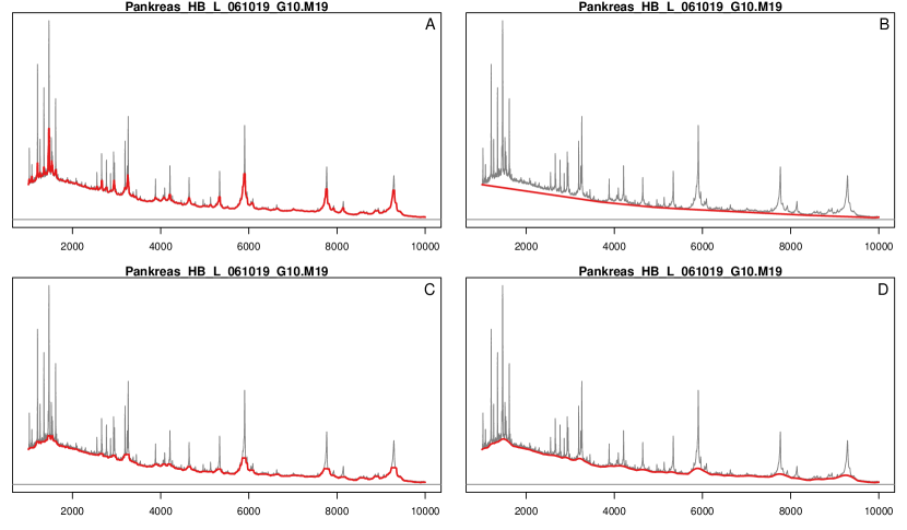
Figure 11.2: Estimated baselines for an raw MALDI-TOF spectrum from Fiedler et al., (2009). The following algorithms were applied: (A) moving median, (B) convex hull, (C) TopHat, (D) SNIP.

11.2.5 Intensity Calibration

The intensity values in mass spectrometry data represent the relative amount of analytes, such as peptides. The measured intensity strongly depends on preanalytical and environmental factors like sample collection, sample storing, room temperature, air humidity, crystallization etc. (Baggerly et al.,, 2004; Leek et al.,, 2010; Leichtle et al.,, 2013).

Further confounders are introduced by so-called batch effects. These are systematical differences that hide the true biological effect and that are caused by different experimental conditions, for instance a different preanalytical processing, measurements on different days by different operators in different laboratories on different devices (Hu et al.,, 2005; Leek et al.,, 2010; Gregori et al.,, 2012).

The systematic errors can be stronger than the real biological effect, and are best minimized already at the stage of data acquisition by strictly adhering to a standardized preanalytical and experimental protocol (Baggerly et al.,, 2004).

Note that unlike in other omics data, such as gene expression data, batch effects and other systematic errors can be the source of shifts both on the $x$-axis (m/z values) and on the $y$-axis (intensity values). Hence, to ensure the validity of any subsequent statistical analysis, great care must be taken to address both of these shift in preprocessing, by intensity calibration (often called normalization) and by peak alignment/warping (see also 11.2.7).

Methods to calibrate peak intensities can be divided into local and global approaches (Meuleman et al.,, 2008). In a local calibration each single spectrum is calibrated on its own, by matching a specified characteristic such as the median, the mean or the Total Ion Current (TIC) (Callister et al.,, 2006; Meuleman et al.,, 2008; Borgaonkar et al.,, 2010). In contrast, global approaches use information across multiple spectra, e.g. employing linear regression normalization (Callister et al.,, 2006), quantile normalization (Bolstad et al.,, 2003), or Probabilistic Quotient Normalization (PQN) (Dieterle et al.,, 2006).

MALDIquant supports two local and one global method. Specifically, it implements the TIC and median calibration as well as PQN. In PQN all spectra are calibrated using the TIC calibration first. Subsequently, a median reference spectrum is created and the intensities in all spectra are standardized using the reference spectrum and a spectrum-specific median is calculated for each spectrum. Finally, each spectrum is rescaled by the median of the ratios of its intensity values and that of the reference spectrum (Dieterle et al.,, 2006).

It has been shown that applying intensity calibration is an essential step in preprocessing (Meuleman et al.,, 2008). Despite its simplicity TIC is often the best choice, especially to account for effects between technical replicates (Shin and Markey,, 2006; Meuleman et al.,, 2008).

11.2.6 Peak Detection

Peak detection is a further step in processing mass spectrometry data, serving both to identify potential relevant features as well as to reduce the dimensionality of the data.

MALDIquant provides the most commonly used peak detection method based on finding local maxima (Yasui et al., 2003a, ; Tibshirani et al.,, 2004; Li,, 2005; Morris et al.,, 2005; Smith et al.,, 2006; Tracy et al.,, 2008). First a window is moved across the spectra and local maxima are detected. Subsequently these local maxima are compared against a noise baseline which is estimated by the Median Absolute Deviation (MAD) or alternatively Friedman’s SuperSmoother (Friedman,, 1984). If a local maximum is above a given Signal-to-Noise Ratio (SNR) it is considered a peak, whereas local maxima below the SNR threshold are discarded (Fig 11.3).

Some authors advocate peak detection methods based on on wavelets (Du et al.,, 2006; Lange et al.,, 2006). These methods are implemented in the Bioconductor R packages MassSpecWavelet and xcms (Smith et al.,, 2006) and thus are readily available if needed.

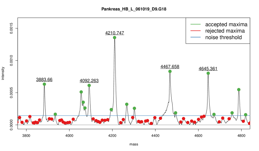
Figure 11.3: Detail view of a MALDI-TOF spectrum from Fiedler et al., (2009). Local maxima are marked with points (red: rejected maxima, green: peaks). The blue line represents the estimated noise baseline as estimated by MAD.

11.2.7 Peak Alignment

As already noted above in Section 11.2.5 not only the intensities but also the m/z values differ across spectra, as result of the many possible sources of variation in the acquisition of mass spectrometry data. Methods to recalibrate the m/z values of the spectra are referred to as peak alignment or warping.

A simple approach is the Correlation Optimized Warping (COW) algorithm (Veselkov et al.,, 2009; Morris et al.,, 2010; Wang et al.,, 2010). COW is based on pairwise comparisons of spectra and maximizes the correlation to find an optimal shift. The advantage of this approach is that correlation is fast to compute and with the use of a reference spectrum the method is also applicable to simultaneous alignment of multiple spectra. However, in actual data the location shifts are typically of a nonlinear nature (He et al.,, 2011), thus methods based on global linear shifts will often be ineffective in achieving an optimal alignment. A possible workaround is to divide the spectrum into several parts and perform local linear alignment instead.

An alternative, and much more flexible approach, is Dynamic Time Warping (DTW) which is based on dynamic programming (Torgrip et al.,, 2003; Toppoo et al.,, 2008; Clifford et al.,, 2009; Kim et al.,, 2011). DTW is a pairwise alignment approach that is guaranteed to find the optimal alignment by comparing each point in the first spectrum to every other point in the second spectrum, and optimizing a distance score. Dynamic programming techniques are used to substantially shortcut computational time by means of an underlying decision tree (e.g. Sakoe and Chiba,, 1978). Still, DTW is a computationally very expensive algorithm that also requires substantial computer memory, especially for multiple alignment.

As a compromise, recently the Parametric Time Warping (PTW) approach has been suggested (Jeffries,, 2005; Lin et al.,, 2005; Bloemberg et al.,, 2010; He et al.,, 2011; Wehrens et al.,, 2015) where a polynomial functions is used to stretch or shrink a spectrum to increase the similarity between them. PTW is a very fast method that is also able to correct for non-linear shifts. As in all previously mentioned method a reference spectrum is necessary for multiple alignment. Note that the use of a reference spectrum requires prior calibration of the intensity values (Smith et al.,, 2013).

Finally, another simple strategy to align peaks is based on clustering respectively creation of bins of similar m/z values (Yasui et al., 2003b, ; Tibshirani et al.,, 2004; Tracy et al.,, 2008). This is a fast and easy to implement approach, and in contrast to DTW, COW and PTW it offers the possibility to align all spectra simultaneously. However, the clustering approach is valid only when there are relatively small shifts around the true peak position, hence this approach is only applicable if there are only mild distortions in the m/z values.

In MALDIquant we use nonlinear warping of peaks (He et al.,, 2011; Wehrens et al.,, 2015). First we align the m/z values of the peaks using PTW and subsequently we employ binning to identify common peak positions across spectra. Note that in contrast to the standard version of PTW we work on peak level rather than on the whole spectrum.

Our peak alignment algorithm in MALDIquant starts by looking for stable peaks, which are defined as high peaks in defined, coarse m/z ranges that are present in most spectra. The m/z of the peaks is averaged and used as reference peak list (also known as anchor or landmark peaks — see Wang et al., (2010). Next, MALDIquant computes a LOcally WEighted Scatterplot Smoothing (LOWESS) curve or polynomial-based function to warp the peaks of each spectra against the reference peaks (Fig. 11.4). As not all reference peaks are found in each spectrum, the number of matched peaks out of all reference peaks is reported by MALDIquant for information.

Due to using the peaks instead of the whole spectral data the alignment approach implemented in MALDIquant is much faster than traditional PTW, still the results are comparable (Fig. 11.5). Another important advantage of our approach is that only m/z values are used for calibration, which implies that our approach does not require perfectly calibrated intensity values as is the case for full spectrum-based alignment methods.

After performing alignment, peak positions of identical features across spectra will become very similar but in general not numerically identical. Thus, as final step grouping of m/z values into bins is needed. For this purpose MALDIquant uses the following simple clustering algorithm: The m/z values are sorted in ascending order and split recursively at the largest gap until all m/z values in the resulting bins are from different samples and their individual m/z values are in a small user-defined tolerance range around their mean. The latter becomes the new m/z value for all corresponding peaks in the associated bin.

Figure 11.4: Example warping function for four different peak lists. The x-axis represents the peak position and the y-axis the difference from the reference peak list. The red line shows the calculated warping function. The number of matched peaks out of all reference peaks is also shown for each spectrum.

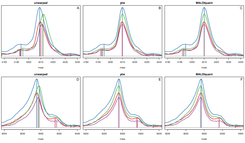
Figure 11.5: Comparison of two peaks (top row and bottom row) present in four MALDI-TOF spectra from Fiedler et al., (2009). (A, D) unaligned; (B, E) warped using the PTW algorithm; (C, F) warped using MALDIquant’s peak based PTW.

11.2.8 Subsequent Statistical Analysis

With peak alignment the task of MALDIquant to transform raw mass spectrometry data into a matrix containing intensity measurements of potentially useful m/z values is complete.

Subsequently, the resulting feature intensity matrix can be used with any preferred univariate or multivariate analysis technique, e.g. to identify peaks that are useful for predicting a desired outcome, or simply to rank features with regard to group separation (e.g. Gibb and Strimmer,, 2015).

In the following section we will describe in detail how such an analysis may be conducted. For more examples please see the MALDIquant homepage.

11.3 Case Study

11.3.1 Dataset

For illustration how to use MALDIquant in practical data analysis we now show in detail how to use the software by application to the mass spectromety data published in Fiedler et al., (2009). The aim of this study was to determine proteomic biomarkers to discriminate patients with pancreas cancer from healthy persons. As part of their study the authors collected serum samples of 40 patients with diagnosed pancreas cancer as well as 40 healthy controls as training dataset. For each sample 4 technical replicates were obtained. These 320 samples were processed following a standardized protocol for serum peptidomics and subsequently analyzed in a linear MALDI-TOF mass spectrometer. For details on the experimental setup we refer to the original study.

Half of the patients and controls were recruited at the University Hospital Heidelberg and the University Hospital Leipzig. Due to the presence of strong batch effects we restrict ourselves to the samples from Heidelberg, leading to a raw data set containing 160 spectra for 40 probands, of which 20 were diagnosed with pancreatic cancer and 20 are healthy controls. Fiedler et al., (2009) found marker peaks at m/z 3884 (double charged) and 7767 (single charged) and correspondingly suggested Platelet Factor 4 (PF4) as potential marker, arguing that PF4 is down-regulated in blood serum of patients with pancreatic cancer.

11.3.2 Preparations

Prior to preprocessing the data we first need to set up our R environment by install the necessary packages, namely MALDIquant (Gibb and Strimmer,, 2012), MALDIquantForeign, sda and crossval, and also download the data set:

install.packages(c("MALDIquant", "MALDIquantForeign",
                   "sda", "crossval"))

## load packages
library("MALDIquant")

Loading required package: methods

This is MALDIquant version 1.13
Quantitative Analysis of Mass Spectrometry Data
See ’?MALDIquant’ for more information about this package.

library("MALDIquantForeign")

## download the raw spectra data (approx. 90 MB)
githubUrl <- paste0("https://raw.githubusercontent.com/sgibb/",
                    "MALDIquantExamples/master/inst/extdata/",
                    "fiedler2009/")
downloader::download(paste0(githubUrl, "spectra.tar.gz"),
                     "fiedler2009spectra.tar.gz")
## download metadata
downloader::download(paste0(githubUrl, "spectra_info.csv"),
                     "fiedler2009info.csv")

11.3.3 Import Raw Data and Quality Control

The first step in the analysis comprises importing the raw data into the R environment. As the raw data set contains both the samples from Heidelberg and Leipzig we filter out the samples from Leipzig, so that our final data set only contains the Heidelberg patients and controls:

## import the spectra
spectra <- import("fiedler2009spectra.tar.gz", verbose=FALSE)

## import metadata
spectra.info <- read.csv("fiedler2009info.csv")

## keep data from Heidelberg
isHeidelberg <- spectra.info$location == "heidelberg"

spectra <- spectra[isHeidelberg]
spectra.info <- spectra.info[isHeidelberg,]

After importing the raw data it is recommend to perform basic sanity checks for quality control. Below, we test whether all spectra contain the same number of data points, are not empty and are regular, i.e. whether the differences between subsequent m/z values are constant:

table(lengths(spectra))

42388
  160

any(sapply(spectra, isEmpty))

[1] FALSE

all(sapply(spectra, isRegular))

[1] TRUE

Next, we ensure that all spectra cover the same m/z range. The ‘trim‘ function automatically determines a suitable common m/z range if it is called without any additional arguments:

spectra <- trim(spectra)

Finally, it is advised to inspect the spectra visually to discover any obviously distorted measurements. Here, for reasons of space we only plot a single spectrum:

plot(spectra[[47]], sub="")

Figure 11.6: Example of a raw, uncalibrated mass spectrum.

11.3.4 Transformation and Smoothing

Next, we perform variance stabilization by applying the square root transformation to the raw data, and subsequently use a 41 point Savitzky-Golay-Filter (Savitzky and Golay,, 1964) to smooth the spectra:

spectra <- transformIntensity(spectra, method="sqrt")

spectra <- smoothIntensity(spectra, method="SavitzkyGolay",
                           halfWindowSize=20)

11.3.5 Baseline Correction

In the next step we address the problem of matrix-effects and chemical noise that result in an elevated baseline. In our analysis we use the SNIP algorithm (Ryan et al.,, 1988) to estimate the baseline for each spectrum. Subsequently, the estimated baseline is subtracted to yield baseline-adjusted spectra:

baseline <- estimateBaseline(spectra[[1]], method="SNIP",
                             iterations=150)
plot(spectra[[1]], sub="")
lines(baseline, col="red", lwd=2)

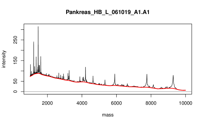
Figure 11.7: Baseline estimated using the SNIP method (red line).

spectra <- removeBaseline(spectra, method="SNIP",
                          iterations=150)
plot(spectra[[1]], sub="")

Figure 11.8: Mass spectrum after baseline correction.

11.3.6 Intensity Calibration and Alignment

After baseline correction we calibrate each spectrum by equalizing the TIC across spectra. After normalizing the intensities we also need to adjust the mass values. This is done by the peak based warping algorithm implemented in MALDIquant. In the example code the function alignSpectra acts as a simple wrapper around more complicated procedures. For a finer control of the underlying procedures the function determineWarpingFunctions may be used alternatively:

spectra <- calibrateIntensity(spectra, method="TIC")
spectra <- alignSpectra(spectra)

Next, we average the technical replicates before we search for peaks and update our meta information accordingly:

avgSpectra <-
  averageMassSpectra(spectra, labels=spectra.info$patientID)
avgSpectra.info <-
  spectra.info[!duplicated(spectra.info$patientID), ]

11.3.7 Peak Detection and Computation of Intensity Matrix

Peak detection is the crucial step to identify features and to reduce the dimensionality of the data. Before performing peak detection we first estimate the noise of selected spectra to investigate suitable settings for the signal-to-noise ratio (SNR):

noise <- estimateNoise(avgSpectra[[1]])
plot(avgSpectra[[1]], xlim=c(4000, 5000), ylim=c(0, 0.002))
lines(noise, col="red")                     # SNR == 1
lines(noise[, 1], 2*noise[, 2], col="blue") # SNR == 2

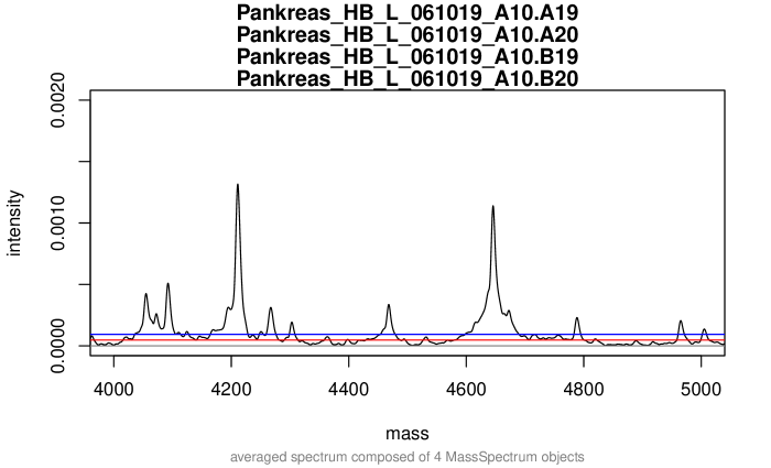
Figure 11.9: Thresholds based on signal to noise ratio (SNR): SNR=1 (red line) and SNR=2 (blue line).

In this case we decide to set a SNR of 2 (blue line) and then run the peak detection algorithm:

peaks <- detectPeaks(avgSpectra, SNR=2, halfWindowSize=20)

plot(avgSpectra[[1]], xlim=c(4000, 5000), ylim=c(0, 0.002))
points(peaks[[1]], col="red", pch=4)

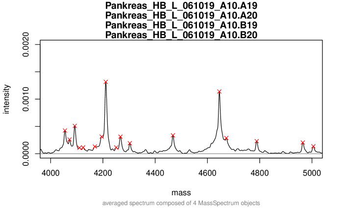
Figure 11.10: Peaks indentified above SNR=2 threshold.

After the alignment the peak positions (mass) are very similar but not numerically identical. Consequently, binning is required to achieve identity:

peaks <- binPeaks(peaks)

In peak detection we choose a very low signal-to-noise ratio to keep as many features as possible. Using the information about class labels we can now filter out false positive peaks, by removing peaks that appear in less than 50 % of all spectra in each group:

peaks <- filterPeaks(peaks, minFrequency=c(0.5, 0.5),
                     labels=avgSpectra.info$health,
                     mergeWhitelists=TRUE)

As final step in MALDIquant we create the feature intensity matrix, and for convenience label the rows with the corresponding patient ID:

featureMatrix <- intensityMatrix(peaks, avgSpectra)
rownames(featureMatrix) <- avgSpectra.info$patientID
dim(featureMatrix)

[1]  40 166

This matrix is the final output of MALDIquant and contains the calibrated intensity values for identified features across all spectra. It forms the basis for higher-level statistical analysis.

11.3.8 Feature Ranking and Classification

The Fiedler et al., (2009) data set contains class labels for each spectrum (healthy versus cancer), hence it is natural to perform a standard classification and feature ranking analysis. A commonly used approach is Fisher’s linear discriminant analysis (LDA), see Mertens et al., (2006) for details and applications to mass spectrometry analysis. Many other classification approaches may also be applied, such as based on Random Forests (Breiman,, 2001) or peak discretization (Gibb and Strimmer,, 2015).

Here, we use a variant of LDA implemented in the R package sda (Ahdesmäki and Strimmer,, 2010). In particular, we use diagonal discriminant analysis (DDA), a special case of LDA with the assumption that the correlation among features (peaks) is negligible. Despite this simplification this approach to classification is very effective, especially in high dimensions (Tibshirani et al.,, 2003). In order to identify the most important class discriminating peaks we use standard $t$-scores, which are the natural variable importance measure in DDA.

As a first step in our analysis we therefore compute the ranking of features by $t$-scores, and list the 10 top-ranking features in Table 11.1:

library("sda")
colnames(featureMatrix) <-
   round(as.double(colnames(featureMatrix)),2)
Ytrain <- avgSpectra.info$health
ddar <- sda.ranking(Xtrain=featureMatrix, L=Ytrain, fdr=FALSE,
                    diagonal=TRUE, verbose=FALSE)

	idx	score	t.cancer	t.control
8936.97	158.00	90.69	9.52	-9.52
4468.07	116.00	80.80	8.99	-8.99
8868.27	157.00	80.06	8.95	-8.95
4494.8	117.00	67.00	8.19	-8.19
8989.2	159.00	66.19	8.14	-8.14
5864.49	135.00	37.56	-6.13	6.13
5906.17	136.00	34.43	-5.87	5.87
2022.94	49.00	33.30	5.77	-5.77
5945.57	137.00	32.66	-5.71	5.71
1866.17	44.00	32.12	5.67	-5.67

Table 11.1: The ten top-ranking peaks as identified in the analysis.

To illustrate that feature selection based on the above feature ranking is indeed beneficial for subsequent analysis we apply hierarchical cluster analysis based on the euclidean distance first to the data set containing all features:

distanceMatrix <- dist(featureMatrix, method="euclidean")

hClust <- hclust(distanceMatrix, method="complete")

plot(hClust, hang=-1)

Figure 11.11: Hierarchical clustering of patient samples using all features.

Next, we repeat the above clustering on the data set containing only the best two top-ranking peaks:

top <- ddar[1:2, "idx"]

distanceMatrixTop <- dist(featureMatrix[, top],
                          method="euclidean")

hClustTop <- hclust(distanceMatrixTop, method="complete")

plot(hClustTop, hang=-1)

Figure 11.12: Hierarchical clustering of patient samples using only the best two top-ranking peaks.

As can be seen by comparison of the two trees, as a result of the feature selection we obtain a nearly perfect split between the Heidelberg pancreas cancer samples (labeled "HP") and the Heidelberg control group (labeled "HC").

The strong predictive capabilities of the first two discovered peaks can be further quantified by conducting a cross-validation analysis to estimate the prediction error. We use the crossval (Strimmer,, 2014) package to perform a 10-fold cross validation using the predictor containing only the two selected peaks:

library("crossval")
# create a prediction function for the cross validation
predfun.dda <- function(Xtrain, Ytrain, Xtest, Ytest,
                        negative) {
  dda.fit <- sda(Xtrain, Ytrain, diagonal=TRUE, verbose=FALSE)
  ynew <- predict(dda.fit, Xtest, verbose=FALSE)$class
  return(confusionMatrix(Ytest, ynew, negative=negative))
}

# set seed to get reproducible results
set.seed(1234)

cv.out <- crossval(predfun.dda,
                   X=featureMatrix[, top],
                   Y=avgSpectra.info$health,
                   K=10, B=20,
                   negative="control",
                   verbose=FALSE)
diagnosticErrors(cv.out$stat)

      acc      sens      spec       ppv       npv       lor
0.9500000 0.9000000 1.0000000 1.0000000 0.9090909       Inf

As a result of the above analysis, we conclude that the identified peaks with mass m/z $8937$ and $4467$ allow for the construction of a very low-dimensional predictor function that is highly effective in separating cancer and control group with both high accuracy as well as high sensitivity.

11.4 Conclusion

The large-scale acquisition of mass spectrometry data is becoming routine in many experimental settings. In MALDIquant we have put together a robust R pipeline for preprocessing these data to allow subsequent high-level statistical analysis. All methods implemented in MALDIquant have been selected both for computational efficiency and for biological validity. In this chapter we have given an overview over the most commonly used procedures of MALDIquant as well as demonstrated their application in detail.

A topic that has not been covered here is Mass Spectrometry Imaging (MSI), which combines spectral measurements with spatial information (Cornett et al.,, 2007). MALDIquant also enables some simple MSI analysis, for practical examples in R we refer to the homepage of MALDIquant at http://strimmerlab.org/software/maldiquant/ as well as the associated web page https://github.com/sgibb/MALDIquantExamples/.

References

- Aebersold and Mann, (2003) Aebersold, R. and Mann, M. (2003). Mass spectrometry-based proteomics. Nature, 422:198–207.
- Ahdesmäki and Strimmer, (2010) Ahdesmäki, M. and Strimmer, K. (2010). Feature selection in omics prediction problems using cat scores and false nondiscovery rate control. The Annals of Applied Statistics, 4(1):503–519.
- Andrew, (1979) Andrew, M. A. (1979). Another Efficient Algorithm for Convex Hulls in Two Dimensions. In Information Processing Letters 9, pages 216–219. Elsevier.
- Baggerly et al., (2004) Baggerly, K. A., Morris, J. S., and Coombes, K. R. (2004). Reproducibility of SELDI-TOF protein patterns in serum: comparing datasets from different experiments. Bioinformatics, 20:777–785.
- Bloemberg et al., (2010) Bloemberg, T. G., Gerretzen, J., Wouters, H. J. P., Gloerich, J., van Dael, M., Wessels, H. J. C. T., van den Heuvel, L. P., Eilers, P. H. C., Buydens, L. M. C., and Wehrens, R. (2010). Improved parametric time warping for proteomics. Chemometrics and Intelligent Laboratory Systems, 104:65–74.
- Bolstad et al., (2003) Bolstad, B. M., Irizarry, R. A., Astrand, M., and Speed, T. P. (2003). A comparison of normalization methods for high density oligonucleotide array data based on variance and bias. Bioinformatics, 19:185–193.
- Borgaonkar et al., (2010) Borgaonkar, S. P., Hocker, H., Shin, H., and Markey, M. K. (2010). Comparison of normalization methods for the identification of biomarkers using MALDI-TOF and SELDI-TOF mass spectra. OMICS, 14:115–126.
- Breiman, (2001) Breiman, L. (2001). Random forests. Machine Learning, 45:5–32.
- Bromba and Ziegler, (1981) Bromba, M. U. A. and Ziegler, H. (1981). Application hints for savitzky-golay digital smoothing filters. Analytical Chemistry, 53(11):1583–1586.
- Callister et al., (2006) Callister, S. J., Barry, R. C., Adkins, J. N., Johnson, E. T., Qian, W.-J., Webb-Robertson, B.-J. M., Smith, R. D., and Lipton, M. S. (2006). Normalization Approaches for Removing Systematic Biases Associated with Mass Spectrometry and Label-Free Proteomics. Journal of Proteome Research, 5:277–286.
- Chambers et al., (2012) Chambers, M. C., Maclean, B., Burke, R., Amodei, D., Ruderman, D. L., Neumann, S., Gatto, L., Fischer, B., Pratt, B., Egertson, J., Hoff, K., Kessner, D., Tasman, N., Shulman, N., Frewen, B., Baker, T. A., Brusniak, M., Paulse, C., Creasy, D., Flashner, L., Kani, K., Moulding, C., Seymour, S. L., Nuwaysir, L. M., Lefebvre, B., Kuhlmann, F., Roark, J., Paape, R., Suckau, D., Hemenway, T., Huhmer, A., Langridge, J., Connolly, B., Chadick, T., Holly, K., Eckels, J., Deutsch, E. W., amnd Katz Moritz, R. L., Agus, D. B., MacCoss, M., Tabb, D. L., and Mallick, P. (2012). A cross-platform toolkit for mass spectrometry and proteomics. Nature biotechnology, 30(10):918–920.
- Clifford et al., (2009) Clifford, D., Montoliu, G. S. I., Rezzi, S., Martin, F.-P., Guy, P., Bruce, S., and Kochhar, S. (2009). Alignment Using Variable Penalty Dynamic Time Warping. Analytical Chemistry, 81:1000–1007.
- Coombes et al., (2005) Coombes, K. R., Tsavachidis, S., Morris, J. S., Baggerly, K. A., Hung, M.-C., and Kuerer, H. M. (2005). Improved peak detection and quantification of mass spectrometry data acquired from surface-enhanced laser desorption and ionization by denoising spectra with the undecimated discrete wavelet transform. Proteomics, 5:4107–4117.
- Cornett et al., (2007) Cornett, D. S., Reyzer, M. L., Chaurand, P., and Caprioli, R. M. (2007). MALDI imaging mass spectrometry: molecular snapshots of biochemical systems. Nat. Meth., 4:828–833.
- Dieterle et al., (2006) Dieterle, F., Ross, A., Schlotterbeck, G., and Senn, H. (2006). Probabilistic quotient normalization as robust method to account for dilution of complex biological mixtures. Application in 1H NMR metabonomics. Analytical Chemistry, 78:4281–4290.
- Du et al., (2006) Du, P., Kibbe, W. A., and Lin, S. M. (2006). Improved peak detection in mass spectrum by incorporating continuous wavelet transform-based pattern matching. Bioinformatics, 22:2059–2065.
- Du et al., (2008) Du, P., Stolovitzky, G., Horvatovich, P., Bischoff, R., Lim, J., and Suits, F. (2008). A noise model for mass spectrometry based proteomics. Bioinformatics, 24:1070–1077.
- Fiedler et al., (2009) Fiedler, G. M., Leichtle, A. B., Kase, J., Baumann, S., Ceglarek, U., Felix, K., Conrad, T., Witzigmann, H., Weimann, A., Schütte, C., Hauss, J., Büchler, M., and Thiery, J. (2009). Serum peptidome profiling revealed platelet factor 4 as a potential discriminating peptide associated with pancreatic cancer. Clinical Cancer Research, 15:3812–3819.
- Friedman, (1984) Friedman, J. H. (1984). A variable span smoother. Technical report, DTIC Document.
- Gammerman et al., (2008) Gammerman, A., Nouretdinov, I., Burford, B., Chervonenkis, A., Vovk, V., and Luo, Z. (2008). Clinical mass spectrometry proteomic diagnosis by conformal predictors. Statistical Applications in Genetics and Molecular Biology, 7.
- Gibb and Strimmer, (2012) Gibb, S. and Strimmer, K. (2012). MALDIquant: a versatile R package for the analysis of mass spectrometry data. Bioinformatics, 28:2270–2271.
- Gibb and Strimmer, (2015) Gibb, S. and Strimmer, K. (2015). Differential protein expression and peak selection in mass spectrometry data by binary discriminant analysis. Bioinformatics, 31:3156–3162.
- Gil and Kimmel, (2002) Gil, J. Y. and Kimmel, R. (2002). Efficient dilation, erosion, opening, and closing algorithms. Pattern Analysis and Machine Intelligence, IEEE Transactions on, 24:1606–1617.
- Gregori et al., (2012) Gregori, J., Villarreal, L., Méndez, O., Sánchez, A., Baselga, J., and Villanueva, J. (2012). Batch effects correction improves the sensitivity of significance tests in spectral counting-based comparative discovery proteomics. Journal of Proteomics, 75(13):3938–3951.
- He et al., (2011) He, Q. P., Wang, J., Mobley, J. A., Richman, J., and Grizzle, W. E. (2011). Self-calibrated warping for mass spectra alignment. Cancer Informatics, 10:65–82.
- House et al., (2011) House, L. L., Clyde, M. A., and Wolpert, R. L. (2011). Bayesian nonparametric models for peak identification in MALDI-TOF mass spectroscopy. The Annals of Applied Statistics, 5:1488–1511.
- Hu et al., (2005) Hu, J., Coombes, K. R., Morris, J. S., and Baggerly, K. A. (2005). The importance of experimental design in proteomic mass spectrometry experiments: some cautionary tales. Briefings in Functional Genomics and Proteomics, 3:322–331.
- Jeffries, (2005) Jeffries, N. (2005). Algorithms for alignment of mass spectrometry proteomic data. Bioinformatics, 21:3066–3073.
- Kim et al., (2011) Kim, S., Koo, I., Fang, A., and Zhang, X. (2011). Smith-Waterman peak alignment for comprehensive two-dimensional gas chromatography-mass spectrometry. BMC Bioinformatics, 12:235.
- Lange et al., (2006) Lange, E., Gröpl, C., Reinert, K., Kohlbacher, O., and Hildebrandt, A. (2006). High-Accuracy Peak Picking of Proteomics Data Using Wavelet Techniques. In Pacific Symposium on Biocomputing, volume 11, pages 243–254.
- Leek et al., (2010) Leek, J. T., Scharpf, R. B., Bravo, H. C., Simcha, D., Langmead, B., Johnson, W. E., Geman, D., Baggerly, K., and Irizarry, R. A. (2010). Tackling the widespread and critical impact of batch effects in high-throughput data. Nature Reviews Genetics, 11:733–739.
- Leichtle et al., (2013) Leichtle, A. B., Dufour, J.-F., and Fiedler, G. M. (2013). Potentials and pitfalls of clinical peptidomics and metabolomics. Swiss Medical Weekly, 143:w13801.
- Li, (2005) Li, X. (2005). PROcess: Ciphergen SELDI-TOF Processing. R package version 1.44.0.
- Lilley et al., (2011) Lilley, K. S., Deery, M. J., and Gatto, L. (2011). Challenges for proteomics core facilities. Proteomics, 11(6):1017–1025.
- Lin et al., (2005) Lin, S. M., Haney, R. P., Campa, M. J., Fitzgerald, M. C., and Patz, E. F. (2005). Characterising phase variations in MALDI-TOF data and correcting them by peak alignment. Cancer Informatics, 1:32–40.
- Liu et al., (2010) Liu, L. H., Shan, B. E., Tian, Z. Q., Sang, M. X., Ai, J., Zhang, Z. F., Meng, J., Zhu, H., and Wang, S. J. (2010). Potential biomarkers for esophageal carcinoma detected by matrix-assisted laser desorption/ionization time-of-flight mass spectrometry. Clinical Chemistry and Laboratory Medicine, pages 855–861.
- Liu et al., (2003) Liu, Q., Krishnapuram, B., Pratapa, P., Liao, X., Hartemink, A., and Carin, L. (2003). Identification of Differentially Expressed Proteins Using MALDI-TOF Mass Spectra. Signals, Systems and Computers, 2003. Conference Record, 2:1323–1327.
- Liu et al., (2009) Liu, Q., Sung, A. H., Qiao, M., Chen, Z., Yang, J. Y., Yang, M. Q., Huang, X., and Deng, Y. (2009). Comparison of feature selection and classification for MALDI-MS data. BMC Genomics, 10(Suppl 1):S3.
- Martens et al., (2011) Martens, L., Chambers, M., Sturm, M., Kessner, D., Levander, F., Shofstahl, J., Tang, W. H., Römpp, A., Neumann, S., Pizarro, A. D., Montecchi-Palazzi, L., Tasman, N., Coleman, M., Reisinger, F., Souda, P., Hermjakob, H., Binz, P.-A., and Deutsch, E. W. (2011). mzML–a community standard for mass spectrometry data. Molecular & Cellular Proteomics, 10:R110.000133.
- Mertens et al., (2006) Mertens, B. J. A., de Noo, M. E., Tollenaar, R. A. E. M., and Deelder, A. M. (2006). Mass spectrometry proteomic diagnosis: enacting the double cross-validatory paradigm. J. Comp. Biol., 13:1591–1605.
- Meuleman et al., (2008) Meuleman, W., Engwegen, J. Y., Gast, M.-C. W., Beijnen, J. H., Reinders, M. J., and Wessels, L. F. (2008). Comparison of normalisation methods for surface-enhanced laser desorption and ionisation (SELDI) time-of-flight (TOF) mass spectrometry data. BMC Bioinformatics, 9:88.
- Morhác, (2009) Morhác, M. (2009). An algorithm for determination of peak regions and baseline elimination in spectroscopic data. Nuclear Instruments and Methods in Physics Research Section A: Accelerators, Spectrometers, Detectors and Associated Equipment, 600:478–487.
- Morris et al., (2010) Morris, J. S., Baggerly, K. A., Gutstein, H. B., and Coombes, K. R. (2010). Statistical contributions to proteomic research. Methods in Molecular Biology, 641:143–166.
- Morris et al., (2005) Morris, J. S., Coombes, K. R., Koomen, J., Baggerly, K. A., and Kobayashi, R. (2005). Feature extraction and quantification for mass spectrometry in biomedical applications using the mean spectrum. Bioinformatics, 21:1764–1775.
- Norris et al., (2007) Norris, J. L., Cornett, D. S., Mobley, J. A., Andersson, M., Seeley, E. H., Chaurand, P., and Caprioli, R. M. (2007). Processing MALDI Mass Spectra to Improve Mass Spectral Direct Tissue Analysis. International Journal of Mass Spectrometry, 260:212–221.
- Pedrioli et al., (2004) Pedrioli, P. G. A., Eng, J. K., Hubley, R., Vogelzang, M., Deutsch, E. W., Raught, B., Pratt, B., Nilsson, E., Angeletti, R. H., Apweiler, R., Cheung, K., Costello, C. E., Hermjakob, H., Huang, S., Julian, R. K., Kapp, E., McComb, M. E., Oliver, S. G., Omenn, G., Paton, N. W., Simpson, R., Smith, R., Taylor, C. F., Zhu, W., and Aebersold, R. (2004). A common open representation of mass spectrometry data and its application to proteomics research. Nature Biotechnology, 22:1459–1466.
- Purohit and Rocke, (2003) Purohit, P. V. and Rocke, D. M. (2003). Discriminant models for high-throughput proteomics mass spectrometer data. Proteomics, 3:1699–1703.
- R Core Team, (2015) R Core Team (2015). R: A Language and Environment for Statistical Computing. R Foundation for Statistical Computing, Vienna, Austria.
- Robb et al., (1989) Robb, R. A., Hanson, D. P., Karwoski, R. A., Larson, A. G., Workman, E. L., and Stacy, M. C. (1989). Analyze: a comprehensive, operator-interactive software package for multidimensional medical image display and analysis. Computerized Medical Imaging and Graphics, 13:433–454.
- Ryan et al., (1988) Ryan, C. G., Clayton, E., Griffin, W. L., Sie, S. H., and Cousens, D. R. (1988). SNIP, a statistics-sensitive background treatment for the quantitative analysis of PIXE spectra in geoscience applications. Nuclear Instruments and Methods in Physics Research Section B: Beam Interactions with Materials and Atoms, 34:396–402.
- Sakoe and Chiba, (1978) Sakoe, H. and Chiba, S. (1978). Dynamic programming algorithm optimization for spoken word recognition. Acoustics, Speech and Signal Processing, IEEE Transactions on, 26:43–49.
- Sauve and Speed, (2004) Sauve, A. C. and Speed, T. P. (2004). Normalization, baseline correction and alignment of high-throughput mass spectrometry data. Proceedings Gensips.
- Savitzky and Golay, (1964) Savitzky, A. and Golay, M. J. E. (1964). Smoothing and Differentiation of Data by Simplified Least Squares Procedures. Analytical Chemistry, 36:1627–1639.
- Schramm et al., (2012) Schramm, T., Hester, A., Klinkert, I., Both, J.-P., Heeren, R. M. A., Brunelle, A., Laprévote, O., Desbenoit, N., Robbe, M.-F., Stoeckli, M., Spengler, B., and Römpp, A. (2012). imzML–a common data format for the flexible exchange and processing of mass spectrometry imaging data. Journal of Proteomics, 75:5106–5110.
- Shin and Markey, (2006) Shin, H. and Markey, M. K. (2006). A machine learning perspective on the development of clinical decision support systems utilizing mass spectra of blood samples. Journal of Biomedical Informatics, 39:227–248.
- Sköld et al., (2007) Sköld, M., Rydén, T., Samuelsson, V., Bratt, C., Ekblad, L., Olsson, H., and Baldetorp, B. (2007). Regression analysis and modelling of data acquisition for SELDI-TOF mass spectrometry. Bioinformatics, 23:1401–1409.
- Smith et al., (2006) Smith, C. A., Want, E. J., O’Maille, G., Abagyan, R., and Siuzdak, G. (2006). XCMS: processing mass spectrometry data for metabolite profiling using nonlinear peak alignment, matching, and identification. Analytical Chemistry, 78:779–787.
- Smith et al., (2013) Smith, R., Ventura, D., and Prince, J. T. (2013). LC-MS alignment in theory and practice: a comprehensive algorithmic review. Briefings in Bioinformatics.
- Strimmer, (2014) Strimmer, K. (2014). crossval: Generic Functions for Cross Validation. R package version 1.0.1.
- Tibshirani et al., (2004) Tibshirani, R., Hastie, T., Narasimhan, B., Soltys, S., Shi, G., Koong, A., and Le, Q.-T. (2004). Sample classification from protein mass spectrometry, by ’peak probability contrasts’. Bioinformatics, 20:3034–3044.
- Tibshirani et al., (2003) Tibshirani, R., Hastie, T., Narsimhan, B., and Chu, G. (2003). Class prediction by nearest shrunken centroids, with applications to DNA microarrays. Statist. Sci., 18:104–117.
- Toppoo et al., (2008) Toppoo, S., Roveri, A., Vitale, M. P., Zaccarin, M., Serain, E., Apostolidis, E., Gion, M., Maiorino, M., and Ursini, F. (2008). MPA: A multiple peak alignment algorithm to perform multiple comparisons of liquid-phase proteomic profiles. Proteomics, 8:250–253.
- Torgrip et al., (2003) Torgrip, R. J. O., Åberg, M., Karlberg, B., and Jacobsson, S. P. (2003). Peak alignment using reduced set mapping. Journal of Chemometrics, 17:573–582.
- Tracy et al., (2008) Tracy, M. B., Chen, H., Weaver, D. M., Malyarenko, D. I., Sasinowski, M., Cazares, L. H., Drake, R. R., Semmes, O. J., Tracy, E. R., and Cooke, W. E. (2008). Precision enhancement of MALDI-TOF MS using high resolution peak detection and label-free alignment. Proteomics, 8:1530–1538.
- van Herk, (1992) van Herk, M. (1992). A fast algorithm for local minimum and maximum filters on rectangular and octagonal kernels. Pattern Recognition Letters, 13:517–521.
- Veselkov et al., (2009) Veselkov, K. A., Lindon, J. C., Ebbels, T. M. D., Crockford, D., Volynkin, V. V., Holmes, E., Davies, D. B., and Nicholson, J. K. (2009). Recursive segment-wise peak alignment of biological (1)h NMR spectra for improved metabolic biomarker recovery. Analytical Chemistry, 81:56–66.
- Wang et al., (2010) Wang, B., Fang, A., Heim, J., Bogdanov, B., Pugh, S., Libardoni, M., and Zhang, X. (2010). DISCO: distance and spectrum correlation optimization alignment for two-dimensional gas chromatography time-of-flight mass spectrometry-based metabolomics. Analytical Chemistry, 82:5069–5081.
- Wehrens et al., (2015) Wehrens, R., Bloemberg, T., and Eilers, P. (2015). Fast parametric time warping of peak lists. Bioinformatics, 15:3063–3065.
- Williams et al., (2005) Williams, B., Cornett, S., Dawant, B., Crecelius, A., Bodenheimer, B., and Caprioli, R. (2005). An Algorithm for Baseline Correction of MALDI Mass Spectra. In Proceedings of the 43rd Annual Southeast Regional Conference - Volume 1, ACM-SE 43, pages 137–142.
- (70) Yasui, Y., McLerran, D., Adam, B., Winget, M., Thornquist, M., and Feng, Z. (2003a). An automated peak-identification/calibration procedure for high-dimensional protein measures from mass spectrometers. Journal of Biomedicine and Biotechnology, 4:242–248.
- (71) Yasui, Y., Pepe, M., Thompson, M. L., Adam, B.-L., Wright, G. L., Qu, Y., Potter, J. D., Winget, M., Thornquist, M., and Feng, Z. (2003b). A data-analytic strategy for protein biomarker discovery: profiling of high-dimensional proteomic data for cancer detection. Biostatistics, 4:449–463.