On comparison of the estimators of the Hurst index and the diffusion coefficient of the fractional Gompertz diffusion process

Abstract

We study some estimators of the Hurst index and the diffusion coefficient of the fractional Gompertz diffusion process and prove that they are strongly consistent and most of them are asymptotically normal. Moreover, we compare the asymptotic behavior of these estimators with the aid of computer simulations.

Keywords: fractional Gompertz diffusion process, Hurst index, diffusion coefficient

¹ Vilnius University, Institute of Mathematics and Informatics, Akademijos 4,

LT-08663 Vilnius, Lithuania

² Vilnius Gediminas Technical University, Faculty of Fundamental Sciences, Saulėtekio al. 11,

LT-10223, Vilnius, Lithuania

1 Introduction

Many applications make use of processes that are described by stochastic differential equations (SDEs). Recently, much attention has been paid to SDEs driven by the fractional Brownian motion (fBm) and to the problems of statistical estimation of model parameters. Statistical aspects of the models driven by the fBm have been studied in many articles. Especially much attention has been paid to the estimation of the parameters of drift. We focus on estimators of the Hurst index and the diffusion coefficient. Recently some new estimators of the Hurst index and of the diffusion coefficient have been proposed (see [1], [3], [14], [13]). This paper aims to compare them using discrete observations of the sample paths of the solution of the SDE.

As the test process we will consider the fractional Gompertz diffusion process (fGd)

$$X_{t}=\int_{0}^{t}(\alpha X_{s}-\beta X_{s}\ln X_{s})\,ds+\sigma\int_{0}^{t}X_{s}\,dB^{H}_{s},\qquad X_{0}=x_{0}>0,\quad 0\leqslant t\leqslant T,$$ (1)

where $\alpha$, $\beta\neq 0$, and $\sigma$ are real parameters and $B^{H}$ is a fBm with the Hurst index $H\in(1/2,1)$. Almost all sample paths of $B^{H}$ have bounded $p$-variation for each $p>1/H$ on $[0,T]$ for every $T>0$. The second integral in (1) is the pathwise Riemann-Stieltjes integral with respect to the process having finite $p$-variation.

The reasons we have chosen fGd as the test process are as follows. Firstly, it is a non-linear process. To the equation (1) it is possible to apply a pathwise approach and use a chain rule for the composition of a smooth function and a function of bounded $p$-variation with $1<p<2$. This approach allows to easily obtain the unique explicit solution of the equation (1) for $H\in(1/2,1)$ in the class of processes, almost all sample paths of which have bounded $p$-variation with $1<p<2$. Secondly, the structure of the increments of fGd allows us to apply a wider class of estimators without imposing additional restrictions on the process. The normalization of quadratic variation by the square of the process value at a fixed point allows us to derive the asymptotic normality of these estimators. The application of this approach allows to consider similar statistics for the equations with time-dependent coefficients. Moreover, in case of the standard Brownian motion, i.e. for $H=1/2$, this process plays an important role in the modeling of population growth.

Dung [7] proved that a class of fractional geometric mean reversion processes expressed by a fractional SDE of the form

$$X_{t}=\int_{0}^{t}(\alpha_{s}X_{s}-\beta_{s}X_{s}\ln X_{s})\,ds+\int_{0}^{t}\sigma_{s}X_{s}\,dW^{H}_{s},\qquad X_{0}=x_{0}>0,\quad 0\leqslant t\leqslant T,$$

where $W^{H}$ is a fractional Brownian motion of the Liouville form, has a unique solution. It follows from his results that, if the coefficients in the equation above are constant, its solution will be of the form

$$X_{t}=\exp\bigg{\{}e^{-\beta t}\ln x_{0}+\alpha\int_{0}^{t}e^{-\beta(t-s)}ds+\sigma\int_{0}^{t}e^{-\beta(t-s)}\,dW^{H}_{s}\bigg{\}}.$$ (2)

In the Appendix it will be shown that the equation (1) has the solution of the same form even without the assumption required by Dung.

In case of the fractional Ornstein-Uhlenbeck process and the geometric Brownian motion a comparison of various estimators of the Hurst index was presented in [11]. The behavior of the estimators based on quadratic variations was compared with that of some of the other known estimators. It should be noted that these estimators are not asymptotically normal. Moreover, only one of the estimators considered in the aforementioned paper is included in the comparison presented in this article.

A reader interested in the existence of the solution of the Gompertz diffusion process with respect to the standard Brownian motion and the estimation of its parameters is encouraged to read [15], [9], [8] and the references therein.

The structure of the paper is as follows. Section 2 presents the estimators considered in the rest of the paper. Section 3 contains the numerical comparison of the estimators’ performance. Sections 4-6 are dedicated to proofs of strong consistency of the considered estimators in case of the fractional Gompertz diffusion process. In the Appendix the existence and uniqueness of the solution of equation (1) is proved.

2 Estimators

In the rest of the paper we will deal with the problem of estimating the Hurst index and the diffusion coefficient of the fractional Gompertz diffusion process based on discrete observations of its sample paths. The estimation of the trend parameters $\alpha$ and $\beta$, although not included in the present paper, can be performed using the least squares method. Using the change of variable $Z_{t}=\ln X_{t}$ the equation (1) can be reduced to the fractional Vasicek model, to which the least squares method is then applied (see, e.g., [17]).

2.1 Hurst index estimators

Let $\pi_{n}=\{\tau^{m_{n}}_{k},\ k=0,\dots,m_{n}\}$, $n\geq 1$, $\mathbb{N}\ni m_{n}\uparrow\infty$, be a sequence of partitions of the interval $[0,T]$. If partition $\pi_{n}$ is uniform then $\tau^{m_{n}}_{k}=\frac{kT}{m_{n}}$ for all $k\in\{0,\ldots,m_{n}\}$. If $m_{n}\equiv n$, we write $t_{k}^{n}$ instead of $\tau_{k}^{m_{n}}$. Let $(X_{t})_{t\in[0,T]}$ be a stochastic process and

$$\Delta^{(1)}X(\tau^{m_{n}}_{k})=X(\tau^{m_{n}}_{k})-X(\tau^{m_{n}}_{k-1}),\qquad\Delta^{(2)}X(\tau^{m_{n}}_{k})=X(\tau^{m_{n}}_{k+1})-2X(\tau^{m_{n}}_{k})+X(\tau^{m_{n}}_{k-1}),$$

$$\qquad k=1,\ldots,m_{n}-(i-1),\quad i=1,2.$$

Denote

$${V^{(i)}_{m_{n},T}=\sum_{k=1}^{m_{n}-(i-1)}\left(\frac{\Delta^{(i)}X(\tau^{m_{n}}_{k})}{X(\tau^{m_{n}}_{k-1})}\right)^{2},}\qquad i=1,2,$$

and

$$W_{n,k}=\sum_{j=-k_{n}+1}^{k_{n}-1}{\big{(}\Delta^{(2)}X_{s^{n}_{j}+t^{n}_{k}}\big{)}^{2}}=\sum_{j=-k_{n}+1}^{k_{n}-1}\left(X_{s^{n}_{j+1}+t^{n}_{k}}-2X_{s^{n}_{j}+t^{n}_{k}}+X_{s^{n}_{j-1}+t^{n}_{k}}\right)^{2},$$

where $s^{n}_{j}=\frac{jT}{m_{n}}$, $m_{n}=nk_{n}$, and $k_{n}=n^{2}$.

Theorem 1

Assume that $X$ is a solution of the fractional Gompertz SDE and $1/2<H<1$. Then

$$\widehat{H}^{(j)}_{n}\xrightarrow{a.s.}{}H,\qquad j=1,2,3,4,$$

and

$$2\ln 2\,\sqrt{n}(\widehat{H}^{(1)}_{n}-H) \xrightarrow{\ d\ }\mathcal{N}(0,\sigma_{*}^{2}),\qquad\sigma_{*}^{2}(H)=\frac{3}{2}\sigma^{2}(H)-2\sigma_{1,2}(H),$$

$$2\sqrt{n}\,\ln\frac{n}{T}\,(\widehat{H}^{(2)}_{n}-H) \xrightarrow{\ d\ }N(0;\sigma^{2}_{H}),$$

$$\sqrt{n}(\widehat{H}^{(3)}_{n}-H) \xrightarrow{\ d\ }\mathcal{N}\bigg{(}0,\sigma_{\ell}^{2}\bigg{(}\mathbf{r},\frac{1}{2}(\mathbf{z}/\sqrt{\mathbf{r}}\,)\bigg{)}\bigg{)}$$

with known variances $\sigma^{2}_{H}$, $\sigma_{1,2}(H)$, $\sigma_{\ell}^{2}\big{(}\mathbf{r},\frac{1}{2}(\mathbf{z}/\sqrt{\mathbf{r}}\,)\big{)}$ defined in section 4.2, where

$$\widehat{H}^{(1)}_{n}= \frac{1}{2}-\frac{1}{2\ln 2}\ln\left(\frac{V^{(2)}_{2n,T}}{V^{(2)}_{n,T}}\right),$$ (3)

$$\widehat{H}_{n}^{(2)}= \frac{1}{2}+\frac{1}{2\ln k_{n}}\ln\left(\frac{2}{n}\sum_{k=2}^{n}\frac{\big{(}\Delta^{(2)}X(t^{n}_{k})\big{)}^{2}}{W_{n,k-1}}\right),$$ (4)

$$\widehat{H}_{n}^{(3)}= -\frac{1}{2}\sum_{j=1}^{\ell}z_{j}\ln\bigg{(}\frac{V^{(2)}_{n_{j},T}}{n_{j}-1}\bigg{)},\qquad n_{j}=r_{j}n,\ r_{j}\in\mathbb{N},\ j=1,\ldots,\ell,\ \ell\neq 1,$$ (5)

$$z_{i}= \frac{y_{i}}{\sum_{i=1}^{\ell}y_{i}^{2}}\quad\mbox{and}\quad y_{i}=\ln r_{i}-\frac{1}{\ell}\sum_{i=1}^{\ell}\ln r_{i},$$

$$\widehat{H}_{n}^{(4)}= \frac{1}{0.1468}\left(\frac{1}{n^{4}-2}\sum_{k=1}^{n^{4}-2}\frac{\left|\Delta^{(2)}X(t^{n^{4}}_{k})+\Delta^{(2)}X(t^{n^{4}}_{k+1})\right|}{\left|\Delta^{(2)}X(t^{n^{4}}_{k})\right|+\left|\Delta^{(2)}X(t^{n^{4}}_{k+1})\right|}-0.5174\right).$$ (6)

Remark 2

The estimators $\widehat{H}^{(i)}_{n}$, $i=1,2,3,4$, were considered in [13], [12], [3], and [1]. The estimator $\widehat{H}^{(2)}_{n}$ can be used to estimate the Hurst index of the generic form of the SDE with an additional restriction on the diffusion coefficient.

2.2 Diffusion coefficient estimators

In this section, we describe four estimators of the diffusion coefficient. The application of the fourth is not explicitly justified, however this can be performed. It was proposed in [3] for the fractional geometric Brownian motion. The aforementioned paper shows it to be a weakly consistent estimator of the diffusion coefficient $\sigma^{2}$.

Theorem 3

Assume that $X$ is a solution of the fractional Gompertz SDE, $1/2<H<1$, and $\widehat{H}_{n}=H+o_{\omega}(\phi(n))$, where $o_{\omega}$ is defined in subsection 5. If $\phi(n)=o\left(\frac{1}{\ln n}\right)$ then

$$\widehat{\sigma}^{\,2}_{1,n}= \frac{n^{2\widehat{H}_{n}-1}}{T^{2\widehat{H}_{n}}}\,V^{(1)}_{n,T}\xrightarrow{a.s.}{}\sigma^{2},$$

$$\widehat{\sigma}^{\,2}_{2,n}= \frac{n^{2\widehat{H}_{n}-1}}{T^{2\widehat{H}_{n}}(4-2^{2\widehat{H}_{n}})}\,V^{(2)}_{n,T}\xrightarrow{a.s.}{}\sigma^{2},$$

$$\widehat{\sigma}^{\,2}_{3,n}= \frac{\sum_{k=1}^{n}\big{(}\Delta^{(1)}X(t^{n}_{k})\big{)}^{2}}{(\tfrac{T}{n})^{2\widehat{H}_{n}}\sum_{k=1}^{n}X^{2}(t^{n}_{k-1})}\xrightarrow{a.s.}{}\sigma^{2}.$$

If $\phi(n)=o\left(\frac{1}{\sqrt{n}\ln n}\right)$ then

$$\sqrt{n}(\widehat{\sigma}^{\,2}_{2,n}-\sigma^{2})\xrightarrow{\ d\ }{\mathcal{N}\big{(}0;\sigma^{4}\sigma^{2}(H)\big{)}},\qquad\mbox{for}\quad 0<H<1,$$

where variance $\sigma^{2}(H)$ are defined in section 4.2.

For the purposes of comparison we shall also consider

$$\widehat{\sigma}_{4,n}=\frac{\exp(\widehat{B})}{(4-2^{2\widehat{H}_{n}^{(3)}})}\,,\qquad\widehat{B}=\frac{1}{2}\bigg{(}\frac{1}{\ell}\sum_{i=1}^{\ell}\ln\bigg{(}\frac{V^{(2)}_{n_{i},T}}{n_{i}-1}\bigg{)}\bigg{)}+\widehat{H}^{(3)}_{n}\bigg{(}\frac{1}{\ell}\sum_{i=1}^{\ell}\ln(n_{i})\bigg{)},$$

where $n_{i}$ and $\widehat{H}^{(3)}_{n}$ are defined in Theorem 1.

Remark 4

The estimators $\widehat{\sigma}^{\,2}_{i,n}$, $i=1,2$, are similar to the estimators used in the book [3] for the evaluation of the diffusion coefficient $\sigma$ of the solutions of linear SDE when $H$ is known. The estimator $\widehat{\sigma}^{\,2}_{3,n}$ is used to estimate the diffusion coefficient of the fractional Ornstein-Uhlenbeck process when $H$ is known (see [17]). We have shown that this restriction can be lifted.

3 Modeling of the estimators

The goal of this section is to describe the numerical simulations that were performed in order to compare the behavior of the estimators considered in this paper.

The sample paths of the fractional Brownian motion, which were further used to construct the sample paths of the fractional Gompertz diffusion process, were simulated using the Wood-Chan circulant matrix embedding method [16]. The values of the constants involved in these simulations were, unless explicitly stated otherwise, $X_{0}=3$, $\alpha=0.5$, $\beta=2$, and $\sigma=1.5$. We considered these sample paths on the unit interval, hence $T=1$. The number of replicates was 300 in all of the considered cases. In what follows we present the dependencies of the estimators both on the true parameter values ($H$, $\sigma$) and on the sample size ($n$). We have also checked for possible dependencies of the estimators of the Hurst index and the diffusion coefficient on the values of the other parameters of the considered equation, namely the drift coefficients $\alpha$ and $\beta$ and the initial condition $X_{0}$. No such dependencies of significant impact have been observed.

3.1 Modeling of the Hurst index estimators

Figures 1 and 2 display, respectively, the dependence of the four estimators of the Hurst index $H$ on its true value and on the sample size (length of the sample path) $n$. In Figure 1, the same sample sizes $n=2^{10}$ were used for all of the considered estimators, which does suggest that the estimators $\widehat{H}^{(4)}_{n}$ and $\widehat{H}^{(2)}_{n}$ would be a-priori less efficient. However, in practical applications the sample size is usually fixed, hence the motivation was to see what kind of performance the considered estimators would show given the exact same number of observations. In Figure 2, the value of the Hurst index was chosen as $H=0.75$. The values of $r_{j}$ were taken to be powers of 2 (more precisely, $r_{j}=2^{j-1}$, $j=1,\,\ldots,\,l$) and, further, the values of $n_{i}$ were taken as $n_{i}=n/r_{i}$ where $n$ denotes the (fixed) maximum sample size length. The value of $l$ was (arbitrarily) taken to be $4$, as simulation results suggested that both considerably smaller (f.e., $2$) and considerably larger (f.e., $log_{2}{n}-1$) values yielded inferior performance. It does appear plausible that for much bigger sample sizes it might be beneficial to increase this value further, however in this study sample sizes exceeding 6400 points were not considered. It can be seen that the performance of the estimator $\widehat{H}_{n}^{(4)}$ is slightly lacking compared to that of the other estimators, which, despite imposing rather different requirements on the sample sizes, show similar precision.

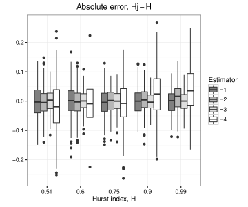
Figure 1: Dependence of the absolute error on $H$

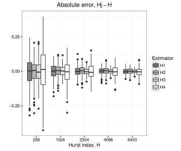
Figure 2: Dependence of the absolute error on $n$

3.2 Modeling of the diffusion coefficient estimators

In order to calculate the estimators $\widehat{\sigma}^{\,2}_{1,n}$, $\widehat{\sigma}^{\,2}_{2,n}$ and $\widehat{\sigma}^{\,2}_{3,n}$ we need to supply them with the estimated values of the Hurst index. In the Figures 3 and 4 presented below, the diffusion coefficient estimator $\widehat{\sigma}^{\,2}_{i,n}$, using the Hurst index estimator $\widehat{H}_{n}^{(j)}$, is denoted as ‘si_hj’, $i,\,j=1,\,2,\,3$. The estimator $\widehat{\sigma}^{\,2}_{4,n}$ is denoted as ‘s4’. The graphs present the relative differences, namely $(\widehat{\sigma}_{i,n}-\sigma)/\sigma$. In Figure 3, the sample size was chosen to be $n=2^{10}$ for all of the considered estimators. In Figure 4, the value of the diffusion coefficient was chosen as $\sigma=1$. It can be seen that the performance of all the considered estimators is roughly similar. The convergence rate of $\widehat{\sigma}^{\,2}_{4,n}$ appears slower, although it seems to perform better for the values of $\sigma$ close to zero. For the other estimators, it appears that using $\widehat{H}_{n}^{(3)}$ yields better numerical characteristics.

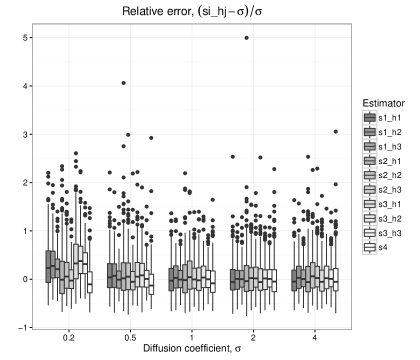
Figure 3: Dependence of the relative error on $\sigma$

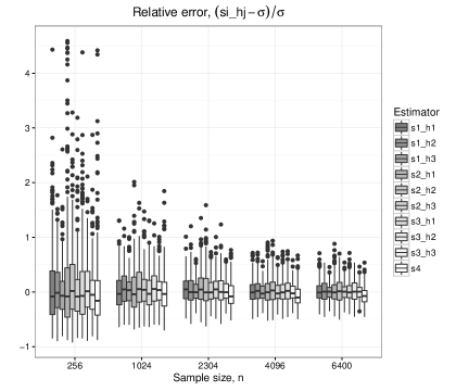
Figure 4: Dependence of the relative error on $n$

4 Preliminaries

4.1 Variation

Let $p>0,-\infty<a<b<\infty$ be fixed and $\mathcal{K}=\{\{x_{0},\dots,x_{n}\}\mid a=x_{0}<x_{1}<\dots<x_{n}=b,n\geq 1\}$ denotes the set of all possible partitions of $[a,b]$. For any $f:[a,b]\to\mathbb{R}$ define

$$v_{p}(f;[a,b])=\sup_{\varkappa\in\mathcal{K}}\sum_{k=1}^{n}\lvert f(x_{k})-f(x_{k-1})\rvert^{p},\qquad V_{p}(f;[a,b])=v_{p}^{\frac{1}{p}}(f;[a,b]).$$

If $v_{p}(f;[a,b])<\infty,$ $f$ is said to have a bounded $p$-variation on $[a,b]$.

In the rest of the paper $\mathcal{W}_{p}([a,b])$ denotes the class of functions on $[a,b]$ with bounded $p$–variation and $C\mathcal{W}_{p}([a,b])=\{f\in\mathcal{W}_{p}([a,b])\mid f$ is continuous$\}$. In case of a fixed interval $[a,b]$ we abbreviate the notations and write $v_{p}(f)$, $V_{p}(f)$, etc. instead of $v_{p}(f;[a,b])$, $V_{p}(f;[a,b])$.

Below we list several facts used in the sequel. For details we refer the reader to [6].

• $p\geq 1\Rightarrow f\mapsto V_{p}(f)$ is a semi-norm on $\mathcal{W}_{p}$.

• $f=const.\Longleftrightarrow V_{p}(f)=0$.

• $f\in\mathcal{W}_{p}\Rightarrow\sup_{x\in[a,b]}\lvert f(x)\rvert<\infty$.

• $p\geq 1,f\in\mathcal{W}_{p}\Rightarrow f\in\mathcal{W}_{q}$ for all $q\geq p$.

• $f,g\in\mathcal{W}_{p}\Rightarrow fg\in\mathcal{W}_{p}$.

• Let $f\in\mathcal{W}_{q}$ and $h\in\mathcal{W}_{p}$ with $p,q\in(0,\infty):1/p+\allowbreak 1/q>1.$ Then an integral $\int_{a}^{b}f\,\mathrm{d}h$ exists as the Riemann–Stieltjes integral provided $f$ and $h$ have no common discontinuities. If the integral exists, the Love–Young inequality

  $$\Bigg{|}\int\limits_{a}^{b}f\,\hbox{\rm d}h-f(y)\big{[}h(b)-h(a)\big{]}\Bigg{|}\leqslant C_{p,q}V_{q}\big{(}f\big{)}V_{p}\big{(}h\big{)}$$ (7)

  holds for all $y\in[a,b]$, where $C_{p,q}=\zeta(p^{-1}+q^{-1})$ and $\zeta(s)=\sum_{n\geqslant 1}n^{-s}$. Moreover,

  $$V_{p}\Bigg{(}\int\limits_{a}^{\hbox{$\bf\cdot$}}f\,\hbox{\rm d}h\Bigg{)}\leq C_{p,q}V_{q,\infty}\big{(}f\big{)}V_{p}\big{(}h\big{)},$$

  where $V_{q,\infty}(f)=V_{q}(f)+\sup_{a\leqslant x\leqslant b}|f(x)|$. Note that $f\mapsto V_{q,\infty}(f)$ is a norm on ${\mathcal{W}}_{q},q\geqslant 1$.

• $h\in C{\mathcal{W}}_{p}\Rightarrow g(y)=\int_{a}^{y}f\,\hbox{\rm d}h$, $y\in[a,b]$, is continuous.

• Let $\phi$ be a locally Lipschitz function and let $f\in\mathcal{W}_{p}([a,b])$. Then the composite function $\phi\circ f$ has bounded $p$-variation, that is, $\phi\circ f\in\mathcal{W}_{p}([a,b])$, where $(\phi\circ f)(x)=\phi(f(x))$.

The chain rule is based on the Riemann–Stieltjes integrals.

Theorem 5 (Chain rule (see [6]))

Let $p\in[1;2)$ and $f=(f_{1},\ldots,f_{d}):[a,b]\to\mathbb{R}^{d}$ be such a function that for each $k=1,\ldots,d$, $f_{k}\in C\mathcal{W}_{p}([a,b])$. Let $g:\mathbb{R}^{d}\to\mathbb{R}$ be a differentiable function with locally Lipschitz partial derivatives $g^{\prime}_{k}$, $k=1,\ldots,d$. Then each $g^{\prime}_{l}\circ f$ is Riemann-Stieltjes integrable with respect to $f_{k}$ and

$$(g\circ f)(b)-(g\circ f)(a)=\sum_{k=1}^{d}\int_{a}^{b}(g_{k}^{\prime}\circ f)\,df_{k}.$$

Proposition 6 (Substitution rule (see [6]))

Let $f,g,h\in C\mathcal{W}_{p}([a,b])$, $1\leqslant p<2$. Then

$$\int_{a}^{b}f(x)\,d\bigg{(}\int_{a}^{x}g(y)\,dh(y)\bigg{)}=\int_{a}^{b}f(x)g(x)\,dh(x).$$

4.2 Several results on fBm

Recall that the fBm $(B^{H}_{t})_{t\in[0,T]}$ with the Hurst index $H\in(0,1)$ is a real-valued continuous centered Gaussian process with the covariance given by

$$\hbox{\bf E}(B^{H}_{t}B^{H}_{s})=\frac{1}{2}\big{(}s^{2H}+t^{2H}-|t-s|^{2H}\big{)}.$$

In order to consider the strong consistency and asymptotic normality of the given estimators we need several facts about $B^{H}$ (see [2], [3], [4], [10]).

Limit results. For consideration of the asymptotic properties of the estimators $\widehat{H}^{(i)}_{n}$, $i=1,2$, we shall use the following results. Let

$$\widehat{V}^{(i)B^{H}}_{n,T}=\frac{n^{2H-1}}{c_{i}}\sum_{k=1}^{n-1}\big{(}T^{-H}{\Delta^{(i)}B^{H}(t^{n}_{k})}\big{)}^{2},\qquad H\neq\frac{1}{2}\,,\quad i=1,2.$$

where $c_{1}=1,c_{2}=4-2^{2H}$. Then

$$\widehat{V}^{(i)B^{H}}_{n,T}\xrightarrow[n\to\infty]{}1\qquad\text{ a.s.}\quad i=1,2;$$

$${\sqrt{n}\left(\widehat{V}^{(1)B^{H}}_{n,T}-1\right)\xrightarrow{\ d\ }\mathcal{N}(0,\sigma^{2}_{*}(H)),\qquad H\in(0,3/4),}$$

$$\sqrt{n}\left(\begin{array}[]{c}\widehat{V}^{(2)B^{H}}_{n,T}-1\\ \widehat{V}^{(2)B^{H}}_{2n,T}-1\\ \end{array}\right)\xrightarrow{\ d\ }\mathcal{N}\left(\left(\begin{array}[]{c}0\\ 0\\ \end{array}\right),\left(\begin{array}[]{cc}\sigma^{2}(H)&\sigma_{1,2}(H)\\ \sigma_{1,2}(H)&\sigma^{2}(H)/2\\ \end{array}\right)\right)$$

with

$${\sigma^{2}_{*}(H)=2\bigg{(}1+2\sum_{j=1}^{\infty}\widehat{\rho}_{H}^{2}(j)\bigg{)},\qquad\widehat{\rho}_{H}(j)=-\frac{1}{2}\big{[}-\lvert j-1\rvert^{2H}+2\lvert j\rvert^{2H}-\lvert j+1\rvert^{2H}\big{]},}$$

$$\sigma^{2}(H)=2\bigg{(}1+2\sum_{j=1}^{\infty}\rho_{H}^{2}(j)\bigg{)},\qquad\sigma_{1,2}(H)=\sum_{j\in\mathbb{Z}}\widetilde{\rho}_{H}^{2}(j)\,,$$

$$\rho_{H}(j)=\frac{-6\lvert j\rvert^{2H}-(\lvert j-2\rvert^{2H}+\lvert j+2\rvert^{2H})+4(\lvert j-1\rvert^{2H}+\lvert j+1\rvert^{2H})}{2(4-2^{2H})},$$

$$\widetilde{\rho}_{H}(j)=\frac{-\lvert j-2\rvert^{2H}+2\lvert j-1\rvert^{2H}+\lvert j\rvert^{2H}-4\lvert j+1\rvert^{2H}+\lvert j+2\rvert^{2H}+2\lvert j+3\rvert^{2H}-\lvert j+4\rvert^{2H}}{2(4-2^{2H})2^{H}}\,.$$

In order to prove the asymptotic normality of the estimator $\widehat{H}^{(3)}_{n}$ we need the following result obtained in [3]. Let $n_{i}=r_{i}n$, $i=1,\ldots,\ell$, where $r_{i},n\in\mathbb{N}$, and $z_{i}$, $i=1,\ldots,\ell$, are defined in Theorem 1. Then

$$\frac{1}{2}\sum_{i=1}^{\ell}\frac{z_{i}}{\sqrt{r_{i}}}\sqrt{n_{i}}\Big{(}\widehat{V}^{(i)B^{H}}_{n_{i},T}-1\Big{)}\xrightarrow{\ d\ }{}\mathcal{N}\bigg{(}0,\sigma_{2,\ell}^{2}\Big{(}\mathbf{r},\frac{1}{2}(\mathbf{z}/\sqrt{\mathbf{r}}\,)\Big{)}\bigg{)},$$

where $\mathbf{r}=(r_{1},\ldots,r_{\ell})$, $\mathbf{z}=(z_{1},\ldots,z_{\ell})$,

$$\sigma_{2,\ell}^{2}(\mathbf{k},\mathbf{d})= \sum_{i=1}^{\ell}\sum_{j=1}^{\ell}d_{i}d_{j}\rho_{2}(k_{i},k_{j}),\qquad\mathbf{k}=(k_{1},\ldots,k_{\ell})\in\mathbb{N}^{\ell},\quad\mathbf{d}=(d_{1},\ldots,d_{\ell})\in\mathbb{R}^{\ell},$$

$$\rho_{2}(k_{i},k_{j})= \frac{1}{\sqrt{k_{i}k_{j}}}\sum_{p=1}^{+\infty}c_{2p,2}^{2}\cdot(2p)!\bigg{(}\sum_{s=0}^{k_{i}-1}\sum_{r=-\infty}^{+\infty}\rho_{k_{i},k_{j}}^{2p}(k_{i}r+k_{j}s)\bigg{)},\qquad c_{2p,2}=\frac{1}{(2p)!}\prod_{i=0}^{p-1}(2-2i),$$

$$\rho_{b,c}(x)= \frac{1}{2(4-2^{2H})}\,(bc)^{-H}\big{[}-\lvert x\rvert^{2H}+2\lvert x-b\rvert^{2H}-\lvert x-2b\rvert^{2H}+2\lvert x+c\rvert^{2H}-4\lvert x+c-b\rvert^{2H}$$

$$+2\lvert x+c-2b\rvert^{2H}-\lvert x+2c\rvert^{2H}+2\lvert x+2c-b\rvert^{2H}-\lvert x+2c-2b\rvert^{2H}\big{]}.$$

If $k_{i}=k_{j}$ then

$$\rho_{2}(k,k)=2\sum_{r=-\infty}^{+\infty}\rho_{H}^{2}(r)=2\bigg{(}1+2\sum_{j=1}^{\infty}\rho_{H}^{2}(j)\bigg{)}.$$

Variation of $B^{H}$. It is known that almost all sample paths of $B^{H}$ are locally Hölder of order strictly less than $H$, $0<H<1$. To be more precise, for all $0<\varepsilon<H$ and $T>0$, there exists a nonnegative random variable $G_{\varepsilon,T}$ such that $\mathbb{E}(|G_{\varepsilon,T}|^{p})<\infty$ for all $p\geq 1$ and

$$sup_{s,t\in[0;T]}|B^{H}_{t}-B^{H}_{s}|\leqslant G_{\varepsilon,T}|t-s|^{H-\varepsilon}\qquad a.s.$$ (8)

Thus $B^{H}\in C\mathcal{W}_{H_{\varepsilon}}([0,T])$, ${H_{\varepsilon}}=\frac{1}{H-\varepsilon}$.

The rate of convergence of the Hurst index.

Theorem 7 ([12], Theorem 3)

For any $t\in[0;T]$ define $r_{nt}=\left[\frac{tn}{T}\right],\rho_{nt}=\frac{r_{nt}}{n}T$ and

$${\widehat{V}_{nt}^{(2)B^{H}}=\frac{n^{2H-1}}{T^{2H-1}(4-2^{2H})}\sum_{k=i}^{r_{nt}}\big{(}\Delta^{(2)}B^{H}(t^{n}_{k})\big{)}^{2}.}$$

Then

$${\sup_{t\in[0;T]}\lvert\widehat{V}_{nt}^{(2)B^{H}}-\rho_{nt}\rvert=O_{\omega}(n^{-1/2}\ln^{1/2}n),}$$ (9)

where $O_{\omega}$ is defined in subsection 5.

5 Properties of the increments of the Gompertz diffusion process

The fractional Gompertz diffusion process $X$ has the explicit solution given by

$$X_{t}=\exp\bigg{\{}e^{-\beta t}\ln x_{0}+\frac{\alpha}{\beta}\big{(}1-e^{-\beta t}\big{)}+\sigma\int_{0}^{t}e^{-\beta(t-s)}dB^{H}_{s}\bigg{\}},\qquad 0\leqslant t\leqslant T.$$

Moreover, it is unique in $C{\mathcal{W}}_{\frac{1}{H-\varepsilon}}([0,T])$ for all $\varepsilon\in\left(0,H-\frac{1}{2}\right)$. The proof of this can be found in the Appendix. Now we will consider the structure of increments of the Gompertz diffusion process.

To avoid cumbersome expressions, we introduce the symbols $O_{\omega}$ and $o_{\omega}$. Let $(Y_{n})$ be a sequence of r. v.s, $\varsigma$ is an a. s. non-negative r. v. and $(a_{n})\subset(0,\infty)$ vanishes. $Y_{n}=O_{\omega}(a_{n})$ means that $|Y_{n}|\leq\varsigma\cdot a_{n}$; $Y_{n}=o_{\omega}(a_{n})$ means that $|Y_{n}|\leq\varsigma\cdot b_{n}$ with $b_{n}=o(a_{n})$. In particular, $Y_{n}=o_{\omega}(1)$ corresponds to the sequence $(Y_{n})$ which tends to $0$ a. s. as $n\to\infty$.

Lemma 8

Suppose that $X$ satisfies $(\ref{e:diflygt})$, $\varepsilon\in(0,H-\frac{1}{2})$ and partition $\pi_{n}$ of the interval $[0,T]$ is uniform. Then the following relations hold:

$$\Delta X_{\tau^{m_{n}}_{k}}= X_{\tau^{m_{n}}_{k-1}}\Big{[}\sigma\Delta B^{H}_{\tau^{m_{n}}_{k}}+O_{\omega}(d_{n})\Big{]}=X_{\tau^{m_{n}}_{k-1}}O_{\omega}\big{(}d_{n}^{H-\varepsilon}\big{)},\qquad k=1,\dots,m_{n},$$ (10)

$$\Delta^{(2)}X_{\tau^{m_{n}}_{k}}= X_{\tau^{m_{n}}_{k-1}}\big{[}\sigma\Delta^{(2)}B^{H}_{\tau^{m_{n}}_{k}}+O_{\omega}\big{(}d_{n}^{2(H-\varepsilon)}\big{)}\big{]},\qquad k=2,\dots,m_{n},$$ (11)

where $d_{n}=\tau^{m_{n}}_{k}-\tau^{m_{n}}_{k-1}$ and $d_{n}\to 0$ as $n\to\infty$. Moreover, $\hbox{\bf E}O_{\omega}(1)<\infty$.

Proof. For the sake of simplicity we will omit the index $m_{n}$ for the points $\tau^{m_{n}}_{k}$. Let the sample path $t\mapsto X_{t}$ be continuous. We first prove (10). Note that

$$\Delta X_{\tau_{k}}=X_{\tau_{k}}-X_{\tau_{k-1}}\quad\mbox{and}\quad X_{\tau_{k}}=X_{\tau_{k-1}}\exp\{\Delta Y_{\tau_{k}}\},$$

where

$$Y_{t}=e^{-\beta t}\ln x_{0}+\frac{\alpha}{\beta}\big{(}1-e^{-\beta t}\big{)}+\sigma\int_{0}^{t}e^{-\beta(t-s)}dB^{H}_{s}.$$

It is clear that

$$\Delta Y_{\tau_{k}}= e^{-\beta\tau_{k-1}}\big{(}e^{-\beta(\tau_{k}-\tau_{k-1})}-1\big{)}\bigg{(}\ln x_{0}-\frac{\alpha}{\beta}+\sigma\int_{0}^{\tau_{k-1}}e^{\beta s}dB^{H}_{s}\bigg{)}$$

$$+\sigma e^{-\beta\tau_{k}}\int^{\tau_{k}}_{\tau_{k-1}}\big{[}e^{\beta s}-e^{\beta\tau_{k}}\big{]}dB^{H}_{s}+\sigma\int^{\tau_{k}}_{\tau_{k-1}}dB^{H}_{s}.$$

From the Chain rule it follows that

$$\int_{0}^{t}e^{\beta s}dB^{H}_{s}=e^{\beta t}B^{H}_{t}-\beta\int_{0}^{t}e^{\beta s}B^{H}_{s}ds.$$

Thus

$$\bigg{|}\int_{0}^{\tau_{k-1}}e^{\beta s}dB^{H}_{s}\bigg{|}=\bigg{|}e^{\beta\tau_{k-1}}B^{H}_{\tau_{k-1}}-\beta\int_{0}^{\tau_{k-1}}e^{\beta s}B^{H}_{s}\,ds\bigg{|}\leqslant e^{|\beta|T}(|\beta|T+1)\sup_{t\leqslant T}\big{|}B^{H}_{t}\big{|}\,.$$

Provided

$${e^{-\beta(\tau_{k}-\tau_{k-1})}=1+O(d_{n}),}$$

it follows that

$$Z_{k-1}:=e^{-\beta\tau_{k-1}}\big{(}e^{-\beta(\tau_{k}-\tau_{k-1})}-1\big{)}\bigg{[}\ln x_{0}-\frac{\alpha}{\beta}+\sigma\int_{0}^{\tau_{k-1}}e^{\beta s}dB^{H}_{s}\bigg{]}=O_{\omega}(d_{n}).$$

Further

$$\bigg{|}\int_{\tau_{k-1}}^{\tau_{k}}\big{[}e^{\beta s}-e^{\beta\tau_{k}}\big{]}dB^{H}_{s}\bigg{|}\leqslant C_{1,H_{\varepsilon}}V_{1}\big{(}e^{\beta\mathbf{\operatorname*{\boldsymbol{\cdot}\rule[0.0pt]{0.0pt}{0.0pt}}}};[\tau_{k-1},\tau_{k}]\big{)}V_{H_{\varepsilon}}\big{(}B^{H};[\tau_{k-1},\tau_{k}]\big{)}$$

$$\leqslant C_{1,H_{\varepsilon}}e^{2|\beta|T}|\beta|(\tau_{k}-\tau_{k-1})V_{H_{\varepsilon}}\big{(}B^{H};[\tau_{k-1},\tau_{k}]\big{)}$$

$$\leqslant C_{1,H_{\varepsilon}}G_{\varepsilon,T}e^{2|\beta|T}|\beta|(\tau_{k}-\tau_{k-1})^{1+H-\varepsilon}=O_{\omega}\big{(}d_{n}^{1+H-\varepsilon}\big{)},$$

since $|e^{x}-1|\leqslant|x|e^{|x|}$ for all $x\in\mathbb{R}$. Consequently,

$$X_{\tau_{k}}= X_{\tau_{k-1}}\exp\Big{\{}Z_{k-1}+O_{\omega}\big{(}d_{n}^{1+H-\varepsilon}\big{)}+\sigma\Delta B^{H}_{\tau^{n}_{k}}\Big{\}}$$

$$= X_{\tau_{k-1}}\Big{[}1+Z_{k-1}+O_{\omega}\big{(}d_{n}^{1+H-\varepsilon}\big{)}+\sigma\Delta B^{H}_{\tau^{n}_{k}}+O_{\omega}\big{(}d_{n}^{2(H-\varepsilon)}\big{)}\Big{]}$$ (12)

and

$${\Delta X_{\tau_{k}}=X_{\tau_{k-1}}\Big{[}Z_{k-1}+O_{\omega}\big{(}d_{n}^{2(H-\varepsilon)}\big{)}+\sigma\Delta B^{H}_{\tau^{n}_{k}}\Big{]}=X_{\tau_{k-1}}O_{\omega}\big{(}d_{n}^{H-\varepsilon}\big{)}.}$$ (13)

Since (see subsection 4.2 and [5])

$$\hbox{\bf E}\Big{(}\sup_{t\leqslant T}\big{|}B^{H}_{t}\big{|}\Big{)}^{p}<\infty\quad\mbox{and}\quad\hbox{\bf E}|G_{\varepsilon,T}|^{p}<\infty$$

for all $p\geqslant 1$, then $\hbox{\bf E}O_{\omega}(1)<\infty$.

Next we prove (11). Taking into account (5) and (13) we get

$$\Delta^{(2)}X_{\tau_{k}}= X_{\tau_{k}}\Big{[}Z_{k}+O_{\omega}\big{(}d_{n}^{2(H-\varepsilon)}\big{)}+\sigma\Delta B^{H}_{\tau^{n}_{k+1}}\Big{]}-X_{\tau_{k-1}}\Big{[}Z_{k-1}+O_{\omega}\big{(}d_{n}^{2(H-\varepsilon)}\big{)}+\sigma\Delta B^{H}_{\tau^{n}_{k}}\Big{]}$$

$$= X_{\tau_{k-1}}\Big{[}1+Z_{k-1}+O_{\omega}\big{(}d_{n}^{2(H-\varepsilon)}\big{)}+\sigma\Delta B^{H}_{\tau^{n}_{k}}\Big{]}\cdot\Big{[}Z_{k}+O_{\omega}\big{(}d_{n}^{2(H-\varepsilon)}\big{)}+\sigma\Delta B^{H}_{\tau^{n}_{k+1}})\Big{]}$$

$$-X_{\tau_{k-1}}\Big{[}Z_{k-1}+O_{\omega}\big{(}d_{n}^{2(H-\varepsilon)}\big{)}+\sigma\Delta B^{H}_{\tau^{n}_{k}}\Big{]}$$

$$= X_{\tau_{k-1}}\Big{[}(Z_{k}-Z_{k-1})+O_{\omega}\big{(}d_{n}^{2(H-\varepsilon)}\big{)}+\sigma\Delta^{(2)}B^{H}_{\tau^{n}_{k}}\Big{]}+X_{\tau_{k-1}}O_{\omega}\big{(}d_{n}^{2(H-\varepsilon)}\big{)}.$$

Since

$$Z_{k}-Z_{k-1}= \big{(}e^{-\beta\tau_{k}}-e^{-\beta\tau_{k-1}}\big{)}\big{(}e^{-\beta d_{n}}-1\big{)}\bigg{[}\ln x_{0}-\frac{\alpha}{\beta}+\sigma\int_{0}^{\tau_{k-1}}e^{\beta s}dB^{H}_{s}\bigg{]}$$

$$+\sigma e^{-\beta\tau_{k}}\big{(}e^{-\beta d_{n}}-1\big{)}\int^{\tau_{k}}_{\tau_{k-1}}e^{\beta s}dB^{H}_{s}=O_{\omega}\big{(}d_{n}^{2(H-\varepsilon)}\big{)},$$

then

$$\bigg{|}\int_{\tau_{k-1}}^{\tau_{k}}e^{\beta s}\,dB^{H}_{s}\bigg{|}\leqslant C_{1,H_{\varepsilon}}V_{1,\infty}\big{(}e^{\beta\mathbf{\operatorname*{\boldsymbol{\cdot}\rule[0.0pt]{0.0pt}{0.0pt}}}};[\tau_{k-1},\tau_{k}]\big{)}V_{H_{\varepsilon}}\big{(}B^{H};[\tau_{k-1},\tau_{k}]\big{)}$$

$$\leqslant 2C_{1,H_{\varepsilon}}e^{|\beta|T}V_{H_{\varepsilon}}\big{(}B^{H};[\tau_{k-1},\tau_{k}]\big{)}$$

$$\leqslant 2C_{1,H_{\varepsilon}}G_{\varepsilon,T}e^{|\beta|T}|\beta|(\tau_{k}-\tau_{k-1})^{H-\varepsilon}=O_{\omega}\big{(}d_{n}^{H-\varepsilon}\big{)}.$$

Thus

$$\Delta^{(2)}X_{\tau_{k}}=X_{\tau_{k-1}}\big{[}\sigma\Delta^{(2)}B^{H}_{\tau^{n}_{k}}+O_{\omega}\big{(}d_{n}^{2(H-\varepsilon)}\big{)}\big{]}.$$

6 Proofs of the main Theorems

6.1 Proof of Theorem 1

1. The convergence of the statistics $\widehat{H}_{n}^{(1)}$ and $\widehat{H}_{n}^{(2)}$ considered in Theorem 1 follows from Lemma 8. Indeed, the asymptotics of the increments of the solution $X$ of the equation (1) are the same as the asymptotics of the increments of the solution of the equation with polynomial drift in [13]. Thus in order to establish the convergence of the estimator $\widehat{H}_{n}^{(1)}$ it suffices to repeat the proof of Theorem 2 in [13]. Further, note that hypotheses $(H)$ and $(H_{1})$ in [14] are satisfied for the solution of the equation (1), i.e.

$$\Delta X_{\tau^{m_{n}}_{k}}= O_{\omega}\big{(}d_{n}^{H-\varepsilon}\big{)},\qquad k=1,\dots,m_{n},$$

$$\Delta^{(2)}X_{\tau^{m_{n}}_{k}}= \sigma X_{\tau^{m_{n}}_{k-1}}\Delta^{(2)}B^{H}_{\tau^{m_{n}}_{k}}+O_{\omega}\big{(}d_{n}^{2(H-\varepsilon)}\big{)},\qquad k=2,\dots,m_{n}.$$

It follows from Lemma 8 and the a.s. continuity of $t\mapsto X_{t}$. Thus it suffices to apply Theorem 2.2 in [14].

2. Now we prove the convergence of the statistic $\widehat{H}_{n}^{(3)}$. The proof presented below follows the outline of the proof of Theorem 3.18 in [3]. By Lemma 8 we get

$$\bigg{(}\frac{n^{H}}{\sigma T^{H}\sqrt{4-2^{2H}}}\bigg{)}^{2}\frac{V^{(2)}_{n,T}}{n-1}= \bigg{(}\frac{n^{H}}{T^{H}\sqrt{4-2^{2H}}}\bigg{)}^{2}\frac{1}{n-1}\sum_{i=1}^{n-1}\bigg{[}\big{(}\Delta^{(2)}_{n}B^{H}_{i}\big{)}^{2}+O_{\omega}\big{(}n^{-3(H-\varepsilon)}\big{)}\bigg{]}$$

$$= \frac{n}{n-1}\,\widehat{V}^{(2)B^{H}}_{n,T}+\frac{1}{4-2^{2H}}\,O_{\omega}\big{(}n^{-H+3\varepsilon}\big{)}\xrightarrow{a.s.}1.$$ (14)

Assume that $3\varepsilon<H-1/2$. By (6.1) and Theorem 7 we get

$$\ln\frac{V^{(2)}_{n,T}}{n-1}= -2H\ln\frac{n}{T}+2\ln\big{(}\sigma\sqrt{4-2^{2H}}\big{)}+\ln\frac{n}{n-1}$$

$$+\ln\bigg{[}\big{(}\widehat{V}^{(2)B^{H}}_{n,T}-1\big{)}+1+\frac{n-1}{n(4-2^{2H})}\,O_{\omega}\big{(}n^{-H+3\varepsilon}\big{)}\bigg{]}$$

$$= -2H\ln\frac{n}{T}+2\ln\big{(}\sigma\sqrt{4-2^{2H}}\big{)}+\ln\frac{n}{n-1}$$

$$+\ln\bigg{[}O_{\omega}(n^{-1/2}\ln^{1/2}n)+1+O_{\omega}\big{(}n^{-H+3\varepsilon}\big{)}\bigg{]}$$

$$= -2H\ln\frac{n}{T}+2\ln\big{(}\sigma\sqrt{4-2^{2H}}\big{)}+O_{\omega}(n^{-1/2}\ln^{1/2}n).$$

Thus

$$\widehat{H}^{(3)}_{n}=-\frac{1}{2}\sum_{i=1}^{\ell}z_{i}\Big{[}-2H\ln\Big{(}\frac{n_{i}}{T}\Big{)}+2\ln\big{(}\sigma\sqrt{4-2^{2H}}\big{)}\Big{]}+O_{\omega}(n^{-1/2}\ln^{1/2}n).$$

We will notice the following properties:

$$\sum_{i=1}^{\ell}y_{i}=0,\qquad\sum_{i=1}^{\ell}z_{i}y_{i}=1,\qquad\sum_{i=1}^{\ell}z_{i}=\frac{\sum_{i=1}^{\ell}y_{i}}{\sum_{i=1}^{\ell}y_{i}^{2}}=0.$$

Using those we get

$$\widehat{H}^{(3)}_{n}= H\sum_{i=1}^{\ell}z_{i}\ln(r_{i}n)-\ln\big{(}\sigma\sqrt{4-2^{2H}}\big{)}\sum_{i=1}^{\ell}z_{i}+O_{\omega}(n^{-1/2}\ln^{1/2}n)$$

$$= H\sum_{i=1}^{\ell}z_{i}\ln(r_{i}n)+O_{\omega}(n^{-1/2}\ln^{1/2}n)$$

$$= H\sum_{i=1}^{\ell}z_{i}\big{[}y_{i}-y_{i}+\ln(r_{i}n)\big{]}+O_{\omega}(n^{-1/2}\ln^{1/2}n)$$

$$= H+H\sum_{i=1}^{\ell}z_{i}\bigg{[}\ln n+\frac{1}{\ell}\sum_{i=1}^{\ell}\ln r_{i}\bigg{]}+O_{\omega}(n^{-1/2}\ln^{1/2}n)=H+O_{\omega}(n^{-1/2}\ln^{1/2}n).$$ (15)

So the estimator $\widehat{H}^{(3)}_{n}$ is strongly consistent.

Now we prove the asymptotic normality of the estimator $\widehat{H}^{(3)}_{n}$. From (6.1) and (6.1) it follows that

$$\widehat{H}^{(3)}_{n}= H-\frac{1}{2}\sum_{i=1}^{\ell}z_{i}\big{(}\widehat{V}^{(2)B^{H}}_{n_{i},T}-1\big{)}+O_{\omega}\big{(}n^{-H+3\varepsilon}\big{)}.$$

Thus

$$\sqrt{n}\big{(}\widehat{H}^{(3)}_{n}-H\big{)}= -\frac{1}{2}\sum_{i=1}^{\ell}\frac{z_{i}}{\sqrt{r_{i}}}\bigg{[}\frac{1}{\sqrt{r_{i}n}}\sum_{k=1}^{r_{i}n-1}\bigg{(}\bigg{(}\frac{(r_{i}n)^{H}}{T^{H}\sqrt{4-2^{2H}}}\,\Delta^{(2)}B^{H}(t^{r_{i}n}_{k})\bigg{)}^{2}-1\bigg{)}\bigg{]}$$

$$+O_{\omega}\big{(}n^{1/2-H+3\varepsilon}\big{)}$$

and we obtain the asymptotic normality of the estimator $\widehat{H}^{(3)}_{n}$ by the application of the limit results from subsection 4.2.

3. It remains to determine the convergence of $\widehat{H}_{n}^{(4)}$. Denote

$$R^{2,n}(X)=\frac{1}{n^{4}-2}\sum_{k=1}^{n^{4}-2}\frac{|\Delta^{(2)}X(\tau^{m_{n}}_{k})+\Delta^{(2)}X(\tau^{m_{n}}_{k+1})|}{|\Delta^{(2)}X(\tau^{m_{n}}_{k})|+|\Delta^{(2)}X(\tau^{m_{n}}_{k+1})|}\,,\qquad\Lambda_{2}(H)=\hbox{\bf E}\frac{|\Delta^{(2)}B^{H}_{1}+\Delta^{(2)}B^{H}_{2}|}{|\Delta^{(2)}B^{H}_{1}|+|\Delta^{(2)}B^{H}_{2}|}\,,$$

where $\Delta^{(2)}B^{H}_{j}=B^{H}(j+1)-2B^{H}(j)+B^{H}(j-1)$, $j=1,2$. This statistic was introduced in [1]. Further on, we will require the following lemma which is a simple modification of Lemma 3.1 in [1]. In this lemma we have lifted the requirement for the random variables $Z_{1}$ and $Z_{2}$ to be independent. This became possible due to the application of less precise estimators of the partial derivatives.

Lemma 9

Let $\psi(x_{1},x_{2})=\frac{|x_{1}+x_{2}|}{|x_{1}|+|x_{2}|}$, $x_{1},x_{2}\in\mathbb{R}$, and let $(Z_{1},Z_{2})$ be a Gaussian vector with zero mean and variance $\hbox{\bf E}Z_{i}^{2}=1$, $i=1,2$. Then for any r. v. $\xi_{i}$, $i=1,2$ with finite second moments we have

$$\hbox{\bf E}\big{|}\psi(Z_{1}+\xi_{1},Z_{2}+\xi_{2})-\psi(Z_{1},Z_{2})\big{|}\leqslant 23\max_{i=1,2}\root 3 \of{\hbox{\bf E}\xi_{i}^{2}}.$$ (16)

Let us proceed to the following claim.

Proposition 10

Let $X$ be the solution of the fractional Gompertz SDE observed at times $\tau^{m_{n}}_{k}=\frac{k}{n^{4}}T$, $k=0,1,\ldots,n^{4}$. Then

$$R^{2,n}(X)\xrightarrow{a.s.}\Lambda_{2}(H)\quad\mbox{as }n\to\infty\quad\mbox{for }H\in(1/2,1)\,.$$

Proof. For the sake of simplicity we will omit the index $m_{n}$ for the points $\tau^{m_{n}}_{k}$ and denote $d_{n}=\frac{T}{n^{4}}$. From Lemma 8 it follows that

$$\Delta^{(2)}X_{\tau_{k}}+\Delta^{(2)}X_{\tau_{k+1}}=\sigma X_{\tau_{k}}\big{[}\Delta^{(2)}B^{H}_{\tau_{k}}+\Delta^{(2)}B^{H}_{\tau_{k+1}}+\zeta_{1}+\zeta_{2}\big{]}$$

for every $\varepsilon\in(0,H-\frac{1}{2})$, where

$$\zeta_{1}=O_{\omega}\big{(}d_{n}^{2(H-\varepsilon)}\big{)},\qquad\zeta_{2}=O_{\omega}\big{(}d_{n}^{H-\varepsilon}\big{)}\big{[}\sigma\Delta^{(2)}B^{H}_{\tau_{k+1}}+O_{\omega}\big{(}d_{n}^{2(H-\varepsilon)}\big{)}\big{]}=O_{\omega}\big{(}d_{n}^{2(H-\varepsilon)}\big{)}.$$

Therefore

$$R^{2,n}(X)=\frac{1}{n^{4}-2}\sum_{k=1}^{n^{4}-2}\frac{|Z_{1}+Z_{2}+\xi_{1}+\xi_{2}|}{|Z_{1}+\xi_{1}|+|Z_{2}+\xi_{2}|}\,,$$

where

$$Z_{1}= \frac{1}{d_{n}^{H}\sqrt{4-2^{2H}}}\,\Delta^{(2)}B^{H}_{\tau_{k}}\,,\qquad Z_{2}=\frac{1}{d_{n}^{H}\sqrt{4-2^{2H}}}\,\Delta^{(2)}B^{H}_{\tau_{k+1}}\,,$$

$$\xi_{1}= \frac{\zeta_{1}}{d_{n}^{H}\sqrt{4-2^{2H}}}\,,\qquad\xi_{2}=\frac{\zeta_{2}}{d_{n}^{H}\sqrt{4-2^{2H}}}$$

and

$$\hbox{\bf E}Z^{2}_{1}=\frac{n^{8H}}{T^{2H}(4-2^{2H})}\,\hbox{\bf E}\big{(}\Delta^{(2)}B^{H}_{\tau_{k}}\big{)}^{2}=1.$$

Let us apply Lemma 9. From the inequality (16) it follows that

$$\hbox{\bf E}\big{|}R^{2,n}(X)-R^{2,n}(B^{H})\big{|}=\bigg{(}\frac{d_{n}^{2(H-2\varepsilon)}}{4-2^{2H}}\bigg{)}^{1/3}\root 3 \of{\hbox{\bf E}O_{\omega}(1)}=d_{n}^{2(H-2\varepsilon)/3}\root 3 \of{\hbox{\bf E}O_{\omega}(1)}.$$

Then the Chebyshev’s inequality yields

$$\hbox{\bf P}\big{(}\big{|}R^{2,n}(X)-R^{2,n}(B^{H})\big{|}>n^{-\beta}\big{)}\leqslant n^{\beta}d_{n}^{2(H-2\varepsilon)/3}\root 3 \of{\hbox{\bf E}O_{\omega}(1)}$$

$$< T^{2(H-2\varepsilon)/3}n^{{\beta-8(H-2\varepsilon)/3}}\root 3 \of{\hbox{\bf E}O_{\omega}(1)}$$

for $\varepsilon\in(0,(H-\frac{1}{2})/2)$, $0<\beta<1/3$ and

$$\sum_{n=1}^{\infty}\hbox{\bf P}\big{(}\big{|}R^{2,n}(X)-R^{2,n}(B^{H})\big{|}>n^{-\beta}\big{)}\leqslant\root 3 \of{\hbox{\bf E}O_{\omega}(1)}\sum_{n=1}^{\infty}n^{\beta-8(H-2\varepsilon)/3}<\infty.$$

According to the Borel–Cantelli Lemma,

$$\hbox{\bf P}\Big{(}\limsup_{n\to\infty}\big{\{}\big{|}R^{2,n}(X)-R^{2,n}(B^{H})\big{|}>n^{-\beta}\big{\}}\Big{)}=0$$

which implies that $R^{2,n}(X)\xrightarrow{a.s.}R^{2,n}(B^{H})$, $n\to\infty$.

The convergence $R^{2,n}(B^{H})\xrightarrow{a.s.}{}\Lambda_{2}(H)$, $n\to\infty$ is established in [1] and holds for $H\in(0;1)$. Clearly, provided $R^{2,n}(X)\xrightarrow{a.s.}R^{2,n}(B^{H})$ and $R^{2,n}(B^{H})\xrightarrow{a.s.}\Lambda_{2}(H)$, $n\to\infty$, it follows that $R^{2,n}(X)\xrightarrow{a.s.}\Lambda_{2}(H)$, $n\to\infty$, which completes the proof.  $\square$

The estimator $\widehat{H}^{(4)}_{n}$ based on $R^{2,n}(X)$ can be obtained using the approximation formula provided in Remark 4.3 [1].

6.2 Proof of Theorem 3

The proof of the convergence of $\widehat{\sigma}^{\,2}_{2,n}$ is analogous to that of $\widehat{c}^{\,2}_{n}$ in [13]. Let us prove that $\widehat{\sigma}^{\,2}_{1,n}\xrightarrow{a.s.}\sigma^{2}$, as $n\to\infty$. Suppose that $d_{n}=\frac{T}{n}$. From Lemma 8 it follows that

$$d_{n}^{-2H}n^{-1}V^{(1)}_{n,T}= \sigma^{2}d_{n}^{-2H}n^{-1}\sum_{i=1}^{n}\big{(}\Delta B^{H}_{t^{n}_{k}}\big{)}^{2}+d_{n}^{-2H}O_{\omega}\big{(}d_{n}^{1+H-\varepsilon)}\big{)}$$

$$= \sigma^{2}\widehat{V}^{(1)B^{H}}_{n,T}+O_{\omega}\big{(}d_{n}^{1-H-\varepsilon}\big{)}.$$

Since

$$\widehat{V}^{(1)B^{H}}_{n,T}\xrightarrow{a.s.}1\quad\mbox{and}\quad\frac{n^{2(H-\widehat{H}_{n})}}{T^{2(H-\widehat{H}_{n})}}=\exp\left\{o_{\omega}(\phi(n))\ln\left(\frac{n}{T}\right)^{2}\right\}\longrightarrow 1,$$ (17)

it can be concluded that

$$\widehat{\sigma}^{\,2}_{1,n}=\frac{n^{2\widehat{H}_{n}-1}}{T^{2\widehat{H}_{n}}}\,V^{(1)}_{n,T}\xrightarrow{a.s.}{}\sigma^{2}\,.$$

Further, let us prove that $\widehat{\sigma}^{\,2}_{3,n}\xrightarrow{a.s.}\sigma^{2}$. Denote $d_{n}=\tfrac{T}{n}$. By (17) it suffices to show that

$$\widetilde{\sigma}^{\,2}_{n}=\frac{\sum_{k=1}^{n}\big{(}\Delta^{(1)}X_{t^{n}_{k}}\big{)}^{2}}{d_{n}^{2H}\sum_{k=1}^{n}X^{2}_{t^{n}_{k-1}}}\xrightarrow{a.s.}{}\sigma^{2}.$$

Notice that

$$\frac{\sum_{k=1}^{n}\big{(}\Delta^{(1)}X_{t^{n}_{k}}\big{)}^{2}}{d_{n}^{2H}\sum_{k=1}^{n}X^{2}_{t^{n}_{k-1}}}=\frac{d_{n}^{1-2H}\sum_{k=1}^{n}\big{(}\Delta^{(1)}X_{t^{n}_{k}}\big{)}^{2}}{d_{n}\sum_{k=1}^{n}X^{2}_{t^{n}_{k-1}}}$$

and

$$d_{n}^{1-2H}\sum_{k=1}^{n}\big{(}\Delta^{(1)}X_{t^{n}_{k}}\big{)}^{2}=\sigma^{2}d_{n}^{1-2H}\sum_{k=1}^{n}X^{2}_{t^{n}_{k-1}}\big{(}\Delta B^{H}_{t^{n}_{k}}\big{)}^{2}+O_{\omega}\big{(}d_{n}^{1-H-\varepsilon}\big{)}.$$ (18)

In order to estimate (18), observe that

$$d_{n}^{1-2H}\sum_{k=1}^{n}X^{2}_{t^{n}_{k-1}}\big{(}\Delta B^{H}_{t^{n}_{k}}\big{)}^{2}=\int_{0}^{T}X^{2}_{t}\,d\widehat{V}^{(1)B^{H}}_{nt}$$

and (see Theorem 7 in [12])

$${d_{n}^{1-2H}\sum_{k=1}^{n}X^{2}_{t^{n}_{k-1}}\big{[}\big{(}\Delta B^{H}_{t^{n}_{k}}\big{)}^{2}-\hbox{\bf E}\big{(}\Delta B^{H}_{t^{n}_{k}}\big{)}^{2}\big{]}}=\int_{0}^{T}X^{2}_{t}\,d\big{(}V^{(1)B^{H}}_{nt}-\hbox{\bf E}V^{(1)B^{H}}_{nt}\big{)}\xrightarrow{a.s.}0.$$

Since

$$d_{n}^{1-2H}\sum_{k=1}^{n}X^{2}_{t^{n}_{k-1}}\hbox{\bf E}\big{(}\Delta B^{H}_{t^{n}_{k}}\big{)}^{2}=d_{n}\sum_{k=1}^{n}X^{2}_{t^{n}_{k-1}}\xrightarrow{a.s.}\int_{0}^{T}X^{2}_{t}\,dt,$$

then

$$\widetilde{\sigma}^{2}_{n}\xrightarrow{a.s.}\sigma^{2}.$$

6.3 The convergence rate of $\widehat{H}_{n}^{(i)},$ $i=1,2,3.$

Theorem 3 makes use of the conditions $\widehat{H}_{n}=H+o_{\omega}(\phi(n))$, $\phi(n)=o\left(\frac{1}{\ln n}\right)$ for strong consistency. Let us show that this indeed holds for $\widehat{H}_{n}^{(i)}$, $i=1,2,3$.

The convergence rate of $\widehat{H}_{n}^{(1)}$. From Lemma 8 and the proof of Theorem 2 in [13] it follows that

$$\widehat{H}_{n}^{(1)}=\widetilde{H}_{n}+O_{\omega}\big{(}n^{-H+3\varepsilon}\big{)},$$

where

$$\widetilde{H}_{n}=\frac{1}{2}-\frac{1}{2\ln 2}{\ln\left(\frac{\widehat{V}^{(2)B^{H}}_{2n,T}}{2^{2H-1}\widehat{V}^{(2)B^{H}}_{n,T}}\right)}=H-\frac{1}{2\ln 2}{\ln\left(\frac{\widehat{V}^{(2)B^{H}}_{2n,T}}{\widehat{V}^{(2)B^{H}}_{n,T}}\right).}$$ (19)

It suffices to consider the convergence rate of the logarithmic term in the equation (19). Using Theorem 7 we get

$${\ln\left(\frac{\widehat{V}^{(2)B^{H}}_{2n,T}}{\widehat{V}^{(2)B^{H}}_{n,T}}\right)}=\ln\bigg{(}\frac{1+O_{\omega}((2n)^{-1/2}\ln^{1/2}(2n))}{1+O_{\omega}(n^{-1/2}\ln^{1/2}n)}\bigg{)}=\ln\big{(}1+o_{\omega}(n^{-1/2}\ln n)\big{)}=o_{\omega}\big{(}n^{-1/2}\ln n\big{)}.$$

Then the statistic $\widetilde{H}_{n}$ has the convergence rate of $o_{\omega}(n^{-1/2}\ln n)$. Consequently, $\widehat{H}_{n}^{(1)}$ satisfies the required condition if $\varepsilon<(H-1/2)/3$.

The convergence rate of $\widehat{H}_{n}^{(2)}$. Denote

$$S_{n,T}:=\frac{2}{nk_{n}^{2H-1}}\sum_{k=2}^{n}\frac{\big{(}\Delta^{(2)}X_{t^{n}_{k}}\big{)}^{2}}{W_{n,k-1}}\,.$$

Then

$$\widehat{H}^{(2)}_{n}=H+\frac{\ln S_{n,T}}{2\ln k_{n}}=H+\frac{\ln S_{n,T}}{4\ln n}\,.$$

Proceeding along the lines of the proof of Theorem 2.2 from [14], it can be concluded that

$$S_{n,T}= \frac{\widetilde{V}^{B^{H}}_{n,T}+O_{\omega}\big{(}n^{-(H-3\varepsilon)}\big{)}}{1+O_{\omega}\left(\sqrt{\frac{\ln n}{k_{n}}}\,\right)+O_{\omega}\left(\frac{m_{n}^{2\varepsilon}}{n^{H-\varepsilon}}\right)}=\frac{\widetilde{V}^{B^{H}}_{n,T}+O_{\omega}\big{(}n^{-(H-3\varepsilon)}\big{)}}{1+O_{\omega}\left(\sqrt{\frac{\ln n}{n^{2}}}\,\right)+O_{\omega}\left(\frac{1}{n^{H-7\varepsilon}}\right)}\,.$$

If $\varepsilon<(H-1/2)/7$, then

$$S_{n,T}=\frac{1+O_{\omega}\Big{(}\sqrt{\frac{\ln n}{n}}\,\Big{)}}{1+O_{\omega}\left(\frac{1}{n^{H-7\varepsilon}}\right)}=1+{O_{\omega}\bigg{(}\frac{\ln n}{\sqrt{n}}\,\bigg{)}.}$$

Hence $\widehat{H}_{n}^{(2)}=H+o_{\omega}(\frac{1}{\ln n})$, if $\varepsilon<(H-1/2)/7$.

The convergence rate of $\widehat{H}_{n}^{(3)}$ was obtained in the proof of Theorem 1.

Appendix

Auxiliary results

Firstly, we consider a non-random integral equation

$$x_{t}=x_{0}+\int_{0}^{t}(\alpha x_{s}-\beta x_{s}\ln x_{s})\,ds+\sigma\int_{0}^{t}x_{s}\,dh_{s},\qquad x_{0}\geqslant 0,\quad\beta\neq 0,\quad 0\leqslant t\leqslant T,$$ (20)

where $h\in C\mathcal{W}_{p}([0,T])$, $1<p<2$, and prove two auxiliary theorems used in the sequel.

Theorem 11

The function

$$x_{t}=\exp\bigg{\{}e^{-\beta t}\ln x_{0}+\frac{\alpha}{\beta}\big{(}1-e^{-\beta t}\big{)}+\sigma\int_{0}^{t}e^{-\beta(t-s)}dh_{s}\bigg{\}},\qquad t\in[0,T],$$ (21)

is an element of $C\mathcal{W}_{p}([0,T])$, $1<p<2$, and satisfies the equation (20).

Proof. We show that $x\in C\mathcal{W}_{p}([0,T])$, $1<p<2$. Let

$$z_{t}=e^{-\beta t}\ln x_{0}+\frac{\alpha}{\beta}\big{(}1-e^{-\beta t}\big{)}+\sigma\int_{0}^{t}e^{-\beta(t-s)}dh_{s}.$$

It is evident that $z\in C\mathcal{W}_{p}([0,T])$, $1<p<2$. Thus by the property of composition of functions (see subsection 4.1) we get $x\in C\mathcal{W}_{p}([0,T])$, $1<p<2$.

Now we verify that the function (21) satisfies (20). This statement can be checked by the application of the Chain rule and the Substitution rule. Namely, let $F(t,x,y)=\exp\{e^{-\beta t}(\ln x_{0}+\alpha x+\sigma y)\}$ and denote

$$A_{t}=\int_{0}^{t}e^{\beta s}ds,\qquad C_{t}=\int_{0}^{t}e^{\beta s}dh_{s}.$$

Note that $x_{t}=F(t,A_{t},C_{t})$ and

$$F(t,A_{t},C_{t})= F(0;0;0)+\int_{0}^{t}\partial_{t}F(s,A_{s},C_{s})dA_{s}+\int_{0}^{t}\partial_{x}F(s,A_{s},C_{s})dC_{s}$$

$$+\int_{0}^{t}\partial_{y}F(s,A_{s},C_{s})ds.$$ (22)

It follows from (Auxiliary results) and Proposition 6

$$x_{t}= x_{0}-\beta\int_{0}^{t}x_{s}\ln x_{s}\,ds+\alpha\int_{0}^{t}x_{s}e^{-\beta s}dA_{s}+\sigma\int_{0}^{t}x_{s}e^{-\beta s}dC_{s}$$

$$= x_{0}-\beta\int_{0}^{t}x_{s}\ln x_{s}\,ds+\alpha\int_{0}^{t}x_{s}\,ds+\sigma\int_{0}^{t}x_{s}\,dh_{s},$$

since

$$dA_{s}=e^{\beta s}ds,\qquad dC_{s}=e^{\beta s}dh_{s}.$$

Theorem 12

The integral equation (20) has a unique solution in $C\mathcal{W}_{p}([0,T])$, $1<p<2$.

Proof. We have already shown that at least one solution $x\in C\mathcal{W}_{p}([0,T])$ exists. Assume it is not unique and $y\in C\mathcal{W}_{p}([0,T])$ is a different one.

Further, one can find a set of points $0=\tau_{0}<\tau_{1}<\tau_{2}<\cdots<\tau_{n}=T$ which satisfies

$$V_{p}(h;[\tau_{k-1},\tau_{k}])\leqslant\big{(}4|\sigma|C_{p,p}\big{)}^{-1}$$

for all $k$. Assume we have proved that $x_{\tau_{k-1}}=y_{\tau_{k-1}}$.

Using the well known inequality $\ln(1+x)\leqslant x$, $x>0$, we get

$$|\ln x_{s}-\ln y_{s}|=\bigg{|}\ln\left(1+\frac{y_{t}-x_{t}}{x_{t}}\right)\bigg{|}\leqslant\bigg{|}\frac{y_{t}-x_{t}}{x_{t}}\bigg{|}\leqslant L_{x,T}\lvert y_{t}-x_{t}\rvert$$

and

$$|\ln x_{s}|\leqslant\Big{|}\ln\Big{(}\max_{0\leqslant t\leqslant T}x_{s}\Big{)}\Big{|}=:\widehat{L}_{x,T}$$

where $L_{x,T}=(\min_{0\leqslant t\leqslant T}\lvert x_{t}\rvert)^{-1}>0$. Then

$$V_{p,\infty}(x-y;[\tau_{k-1},\tau_{k}])= V_{p,\infty}(x-y-(x_{\tau_{k-1}}-y_{\tau_{k-1}});[\tau_{k-1},\tau_{k}])$$

$$\leqslant 2|\alpha|\int_{\tau_{k-1}}^{\tau_{k}}|x_{t}-y_{t}|\,dt+2|\beta|\int_{\tau_{k-1}}^{\tau_{k}}|x_{t}\ln x_{t}-y_{t}\ln y_{t}|\,dt$$

$$+2|\sigma|C_{p,p}V_{p,\infty}(x-y;[\tau_{k-1},\tau_{k}])V_{p}(h;[\tau_{k-1},\tau_{k}])$$

$$\leqslant 2\big{(}|\alpha|+|\beta|\widehat{L}_{x,T}+|\beta|L_{x,T}\big{)}\int_{\tau_{k-1}}^{\tau_{k}}|x_{t}-y_{t}|\,dt$$

$$+2|\sigma|C_{p,p}V_{p,\infty}(x-y;[\tau_{k-1},\tau_{k}])V_{p}(h;[\tau_{k-1},\tau_{k}])$$

and

$$V_{p,\infty}(x-y;[\tau_{k-1},\tau_{k}])\leqslant 4\big{(}|\alpha|+|\beta|\widehat{L}_{x,T}+|\beta|L_{x,T}\big{)}\int_{\tau_{k-1}}^{\tau_{k}}|x_{t}-y_{t}|\,dt$$

$$\leqslant 4\big{(}|\alpha|+|\beta|\widehat{L}_{x,T}+|\beta|L_{x,T}\big{)}\int_{\tau_{k-1}}^{\tau_{k}}V_{p,\infty}(x-y;[\tau_{k-1},t])\,dt.$$

Therefore by Gronwall’s inequality $V_{p,\infty}(x-y;[\tau_{k-1},\tau_{k}])=0$ and we can conclude that $x=y$ on $[\tau_{k-1},\tau_{k}]$. Since $x_{\tau_{0}}=x_{0}=y_{\tau_{0}}$ the claim of the theorem follows from the repetitive application of the reasoning explained above.

The solution of SDE

Since almost all sample paths of $B^{H}$, $1/2<H<1$, are continuous and have bounded $H_{\varepsilon}=\frac{1}{H-\varepsilon}$-variation, $\varepsilon\in(0,H-1/2)$, the pathwise Riemann-Stieltjes integral $\int_{0}^{t}X_{s}\,dB^{H}_{s}$ exists for $X\in C\mathcal{W}_{H_{\varepsilon}}([0,T])$. So SDE (1) is well defined for almost all $\omega$ and the obtained result for a non-random integral equation can be applied to an equation driven by fBm.

Theorem 13

Suppose that $X_{0}>0$ and $m\geqslant 2$. The stochastic process

$$X_{t}=\exp\bigg{\{}e^{-\beta t}\ln x_{0}+\frac{\alpha}{\beta}\big{(}1-e^{-\beta t}\big{)}+\sigma\int_{0}^{t}e^{-\beta(t-s)}dB^{H}_{s}\bigg{\}},\qquad\beta\neq 0,\quad 0\leqslant t\leqslant T.$$

for almost all $\omega$ belongs to $C\mathcal{W}_{H_{\varepsilon}}([0,T])$ and is the unique solution of (1).

Acknowledgment. The authors would like to thank the referees for many valuable comments which allowed us to improve this paper.

References

• [1] J.-M. Bardet, D. Surgailis, Measuring the roughness of random paths by increment ratios. // Bernoulli, 17(2), 2011, 749-780
• [2] A. Bégyn, Asymptotic development and central limit theorem for quadratic variations of Gaussian processes, Bernoulli, 13(3) (2007), 712-753.
• [3] C. Berzin, A. Latour, J.R. León, Inference on the Hurst Parameter and the Variance of Diffusions Driven by Fractional Brownian Motion, Lecture Notes in Statistics 216, Springer (2014).
• [4] J.F. Coeurjolly, Estimating the parameters of a fractional Brownian motion by discrete variations of its sample paths, Statistical Inference for Stochastic Processes, 4 (2001), 199-227.
• [5] K. Dȩbicki, A. Tomanek, Estimates for moments of supremum of reflected fractional Brownian motion. // arXiv preprint arXiv:0912.3117, 2009.
• [6] R.M. Dudley, R. Norvaiša, Concrete Functional Calculus. Springer Monographs in Mathematics. New York, Springer (2011).
• [7] N.T. Dung, Fractional Geometric Mean Reversion Processes, J. Math. Anal. Appl., vol. 330. pp. 396-402, 2011.
• [8] Ferrante L, Bompadre S., Possati L., Leone L., Parameter estimation in a Gompertzian Stochastic Model for tumor growth, Biometrics 56(4) (2000) 1076-1081.
• [9] R. Gutiérrez, A. Nafidi and R. Gutiérrez Sánchez, Inference in the stochastic Gompertz diffusion model with continuous sampling. In VIII Journées Zaragoza-Pau de Mathématiques Appliquées et de Statistiques: Jaca, Spain, September 15-17, 2003, 347-353. Prensas Universitarias de Zaragoza 2003.
• [10] J. Istas, G. Lang, Quadratic variations and estimation of the local Hölder index of a Gaussian process. Ann. Inst. Henri Poincaré, Probab. Stat., 33 (1997), 407-436.
• [11] K. Kubilius, D. Melichov, On comparison of the estimators of the Hurst index of the solutions of stochastic differential equations driven by the fractional Brownian motion, Informatica 22(1) (2011) 97-114.
• [12] K. Kubilius, Y. Mishura. The rate of convergence of estimate for Hurst index of fractional Brownian motion involved into stochastic differential equation. // Stochastic processes and their applications, 122(11), 2012, p. 3718-3739.
• [13] K. Kubilius, V. Skorniakov, D. Melichov, Estimation of parameters of SDE driven by fractional Brownian motion with polynomial drift, Journal of Statistical Computation and Simulation, http://dx.doi.org/10.1080/00949655.2015.1095301 (online).
• [14] K. Kubilius, V. Skorniakov, On some estimators of the Hurst index of the solution of SDE driven by a fractional Brownian motion. // Statistics and Probability Letters, 109, 2016, p. 159-167
• [15] C.H. Skiadas, Exact Solutions of Stochastic Differential Equations: Gompertz, Generalized Logistic and Revised Exponential, Methodol Comput Appl Probab (2010) 12:261-270.
• [16] A. Wood, G. Chan, Simulation of Stationary Gaussian Processes in $[0,1]^{d}$. // Journal of Computational and Graphical Statistics, 4(3), 1994, p. 409-432.
• [17] W. Xiao, W. Zhang, X. Zhang, and X. Chen, The valuation of equity warrants under the fractional Vasicek process of the short-term interest rate, Physica A: Statistical Mechanics and its Applications, 394, 2014, p. 320-337.