The two-jet rate in $e^{+}e^{-}$ at next-to-next-to-leading-logarithmic order

Abstract

We present the first next-to-next-to-leading logarithmic resummation for the two-jet rate in $e^{+}e^{-}$ annihilation in the Durham and Cambridge algorithms. The results are obtained by extending the ARES method to observables involving any global, recursively infrared and collinear safe jet algorithm in $e^{+}e^{-}$ collisions. As opposed to other methods, this approach does not require a factorization theorem for the observables. We present predictions matched to next-to-next-to-leading order, and a comparison to LEP data.

Jet rates and event shapes in electron-positron collisions played a crucial role in establishing QCD as the theory of strong interactions, see e.g. Altarelli:1989ue ; Bethke:1992gh . Nowadays, these observables are still among the most precise tools used for accurate extractions of the main parameter of the theory, the strong coupling constant $\alpha_{s}$. These fits rely on comparing precise measurements of distributions to accurate perturbative predictions supplemented with a modelling of non-perturbative effects. Fixed order predictions up to next-to-next-to-leading order (NNLO) for $e^{+}e^{-}\to$ 3 jets are available GehrmannDeRidder:2007hr ; GehrmannDeRidder:2008ug ; Weinzierl:2008iv ; Weinzierl:2009ms ; DelDuca:2016ily . However, they are not reliable in the two-jet limit, where the cross section is dominated by multiple soft-collinear emissions. In this region, terms as large as ${\cal O}(\alpha_{s}^{n}L^{2n})$ (where $L=\ln(1/v)$) appear to all orders in the integrated distributions of an observable $v$ that vanishes in the two-jet limit. These large logarithms invalidate fixed-order expansions in the coupling constant and reliable predictions can only be obtained by resumming the logarithmically enhanced terms to all orders in $\alpha_{s}$. Double logarithmic terms ${\cal O}(\alpha_{s}^{n}L^{2n})$ are known to exponentiate (see e.g. ref. Catani:1991hj ) and give rise to a well-known Sudakov peak in differential distributions, where most of the data lies. For exponentiating observables, it is customary to define leading logarithms (LL) as terms of the form $\alpha_{s}^{n}L^{n+1}$ for the logarithm of the cross section, next-to-leading logarithms (NLL) as $\alpha_{s}^{n}L^{n}$, next-to-next-to-leading logarithms (NNLL) as $\alpha_{s}^{n}L^{n-1}$. For several $e^{+}e^{-}$ observables, NNLL predictions (in some cases even beyond) are nowadays available deFlorian:2004mp ; Becher:2008cf ; Chien:2010kc ; Becher:2012qc ; Hoang:2014wka ; Banfi:2014sua ; Becher:2015lmy ; Frye:2016okc ; Frye:2016aiz . On the contrary, two-jet rates have been described only at NLL accuracy so far Banfi:2001bz . The lack of precise theory predictions close to the peak of the distribution limits the fit range that can be used to extract $\alpha_{s}$ and results in larger perturbative uncertainties in the latter. Among the existing fits, extractions from the thrust and $C$-parameter Abbate:2010xh ; Hoang:2015hka ; Gehrmann:2012sc that rely on the most precise theory predictions show a tension with the world average determination of the coupling Bethke:2015etp . One of the issues is that at LEP energies non-perturbative corrections are sizeable, and the separation between perturbative and non-perturbative effects is subtle. Fits of $\alpha_{s}$ from the two-jet rate have been so far performed based on pure NNLO Dissertori:2009qa , or NNLO+NLL Bethke:2008hf ; Dissertori:2009ik ; OPAL:2011aa results. Owing to the different sensitivity to non-perturbative effects, an extraction of $\alpha_{s}$ from NNLO+NNLL predictions for the two-jet rate and from the vast amount of high-precision LEP data Heister:2003aj ; Abdallah:2003xz ; Adeva:1992gv ; Achard:2004sv ; Abbiendi:2004qz can shed light on this disturbing tension. The aim of this letter is to present the first NNLL+NNLO results for this observable.

The two-jet rate is defined through a clustering algorithm based on an ordering $v_{ij}$ and a test variable $y_{ij}$. In the Durham algorithm Catani:1991hj the two variables coincide

$$y_{ij}^{(D)}=v_{ij}^{(D)}=2\frac{{\rm min}\{E_{i},E_{j}\}^{2}}{Q^{2}}\left(1-\cos\theta_{ij}\right)\,,$$ (1)

where $\theta_{ij}$ is the angle between (pseudo-)particles $i$ and $j$, $E_{i}$ is the energy of the (pseudo-)particle $i$, and $Q$ is the center-of-mass energy. The clustering procedure selects the pair with the smallest $y_{ij}^{(D)}$. If the latter is smaller than a given $y_{\rm cut}$, the two particles are recombined into a pseudo-particle according to some recombination scheme. Otherwise, the clustering sequence stops, and the number of jets is defined as the number of pseudo-particles left. In the Cambridge algorithm Dokshitzer:1997in ; Bentvelsen:1998ug , the test and ordering variables differ, and are defined by

$$y_{ij}^{(C)}=y_{ij}^{(D)}\,,\qquad v_{ij}^{(C)}=2\left(1-\cos\theta_{ij}\right)\,.$$ (2)

The clustering procedure selects the pair with the smallest $v_{ij}^{(C)}$. If the corresponding $y_{ij}^{(C)}$ is smaller than $y_{\rm cut}$, the two particles are recombined into a pseudo-particle, otherwise the softer particle becomes a jet. This is commonly referred to as the soft freezing mechanism. The procedure stops when no pseudo-particles are left. The angular-ordered (AO) version of the Durham algorithm Dokshitzer:1997in works identically to the Cambridge algorithm, but without the freezing mechanism. The three-jet resolution parameter $y_{3}$ is defined as the minimum $y_{\rm cut}$ that produces two jets. The two-jet rate is the cumulative integral of the $y_{3}$ distribution, normalized to the total cross section $\sigma$:

$$\Sigma(y_{\rm cut})=\frac{1}{\sigma}\int_{0}^{y_{\rm cut}}dy_{3}\frac{d\sigma(y_{3})}{dy_{3}}\,.$$ (3)

The resummation technique formulated in ref. Banfi:2014sua for event shapes does not require the factorization of the singular soft and collinear modes in the observable’s definition, but it rather relies on a property known as recursive infrared and collinear (rIRC) safety Banfi:2004yd . In this sense, the all-order treatment does not require a factorization theorem for the observable. In the following, we present an extension of the above method to jet observables and apply it to the two-jet rate in the Durham and Cambridge algorithm.

Let $y_{3}(\{\tilde{p}\},k_{1},\dots,k_{n})$ denote a three-jet resolution which depends on all $n+2$ final-state momenta, where $\{\tilde{p}\}$ indicates the two Born momenta recoiling against the secondary emissions $k_{1},\dots,k_{n}$. Each parton $k_{i}$ is emitted off leg $\ell_{i}=1,2$. The essence of the procedure described in ref. Banfi:2014sua is that the NLL cross section is given by all-order configurations made of partons independently emitted off the Born legs and widely separated in angle Banfi:2001bz . The NNLL corrections are obtained by correcting a single parton of the above ensemble to account for all kinematic configurations that give rise to NNLL effects Banfi:2014sua . The two-jet rate at NNLL can be written as

$$\Sigma(y_{\rm cut})=\,e^{-R_{\text{NNLL}}(y_{\rm cut})}\left[\mathcal{F}_{\text{NLL}}(y_{\rm cut})\right.$$

$$\left.+\frac{\alpha_{s}(\mu_{R})}{\pi}\delta{\mathcal{F}}_{\rm NNLL}(y_{\rm cut})\right],$$

$$\delta{\mathcal{F}}_{\rm NNLL}(y_{\rm cut})=\,\delta\mathcal{F}_{\rm clust}+\delta\mathcal{F}_{\rm correl}+\delta\mathcal{F}_{\rm sc}$$

$$\hskip 59.75095pt+\delta\mathcal{F}_{\rm hc}+\delta\mathcal{F}_{\rm rec}+\delta\mathcal{F}_{\rm wa}\,,$$ (4)

where $\mu_{R}$ is the renormalization scale, and the physical origin of the various contributions is discussed in the following. The NNLL Sudakov radiator $R_{\text{NNLL}}(y_{\rm cut})$ expresses the no-emission probability above $y_{\rm cut}$ and hence embodies the cancellation of infrared and collinear divergences between the virtual corrections to the Born process and the unresolved real emissions as defined in ref. Banfi:2014sua . As such, it is inclusive over QCD radiation and it is universal for all observables featuring the same scaling in the presence of a single soft and collinear emission. Since, in the soft-collinear limit, $y_{3}(\{\tilde{p}\},k)=(k_{t}/Q)^{2}$, where $k_{t}$ is the emission’s transverse momentum with respect to the emitting quark-antiquark pair, one can obtain $R_{\text{NNLL}}(y_{\rm cut})$ from appendix B of ref. Banfi:2014sua by setting $a=2$ and taking the limit $b_{\ell}\to 0$. All remaining contributions in eq. (The two-jet rate in $e^{+}e^{-}$ at next-to-next-to-leading-logarithmic order) arise from resolved real radiation in different kinematical regions. In particular, the terms $\mathcal{F}_{\text{NLL}},\delta\mathcal{F}_{\rm sc},\delta\mathcal{F}_{\rm clust},\delta\mathcal{F}_{\rm correl}$ originate from soft and collinear emissions. The function $\mathcal{F}_{\text{NLL}}$ is the only NLL correction to the radiator, and it is defined in terms of soft and collinear gluons independently emitted off the hard legs, and widely separated in rapidity. At NLL, the upper rapidity bound is the same for all emissions and approximated by $\ln(1/\sqrt{y_{\rm cut}})$. The soft-collinear term $\delta\mathcal{F}_{\rm sc}$ arises from considering the NNLL effects of the running coupling in the soft matrix element, as well as restoring the exact rapidity bound for a single soft-collinear emission. The two functions $\delta\mathcal{F}_{\rm clust}$ and $\delta\mathcal{F}_{\rm correl}$ account for configurations in which at most two emissions are close in rapidity, and produce a pure abelian clustering correction ($\delta\mathcal{F}_{\rm clust}$) and a non-abelian correlated ($\delta\mathcal{F}_{\rm correl}$) one. The hard-collinear ($\delta\mathcal{F}_{\rm hc}$) and recoil ($\delta\mathcal{F}_{\rm rec}$) corrections describe configurations where one emission of the ensemble is collinear, but hard. In particular, $\delta\mathcal{F}_{\rm hc}$ takes into account the correct approximation of matrix elements in this region, while $\delta\mathcal{F}_{\rm rec}$ describes NNLL kinematical recoil effects in the observable. Finally, the wide-angle correction $\delta\mathcal{F}_{\rm wa}$ encodes configurations in which a single emission of the ensemble is soft and emitted at wide angles.

All of the above corrections are obtained following a method close in spirit to an expansion by regions, i.e. by taking the proper kinematical limits in the squared amplitudes, the phase space and the observable constraint $\Theta\left(y_{\rm cut}-y_{3}(\{\tilde{p}\},k_{1},\dots,k_{n})\right)$. This leads to the definition of a tailored and simplified version of the observable - in our case a clustering algorithm - obtained from the exact one by taking the appropriate asymptotic limit in each kinematic region. The NNLL corrections that appear in eq. (The two-jet rate in $e^{+}e^{-}$ at next-to-next-to-leading-logarithmic order) have already been derived in the context of event-shapes resummations Banfi:2014sua , with the exception of the clustering correction $\delta\mathcal{F}_{\rm clust}$ which is absent for event-shapes, and the soft-collinear correction $\delta\mathcal{F}_{\rm sc}$ which is generalized in this letter. In the following we discuss the algorithms necessary to compute the NLL multiple emission function $\mathcal{F}_{\text{NLL}}$ and the new correction $\delta\mathcal{F}_{\rm clust}$. The remaining algorithms are obtained following the same strategy of taking the asymptotic limit in the region considered in each correction. They are reported in ref. BMMZadditional both for the Durham and for the Cambridge. We will first discuss the case of the Durham algorithm, and we will eventually obtain the Cambridge result as a trivial case of the discussion that follows.

We start by recalling the calculation of $\mathcal{F}_{\text{NLL}}$, which is determined by an ensemble of soft-collinear, strongly angular-ordered partons emitted independently off the Born legs. For soft emissions, recoil effects are negligible and all transverse momenta can be computed with respect to the emitting quark-antiquark pair. For each emission $k_{i}$ we define the rapidity fraction with respect to the emitting leg $\ell_{i}$ as $\xi_{i}^{(\ell_{i})}=|\eta_{i}|/\ln(1/\sqrt{y_{\rm cut}})$, where $\ln(1/\sqrt{y_{\rm cut}})$ is the NLL rapidity bound, common to all emissions at this order. For this ensemble, the Durham algorithm is approximated by the following simplified version, $\overline{y}_{3}^{\rm sc}(\{\tilde{p}\},k_{1},\dots,k_{n})$ Banfi:2001bz :

• Find the pseudo-particle $k_{I}$ with the smallest value of $\overline{y}_{3}^{\rm sc}(\{\tilde{p}\},k_{I})=(k_{tI}/Q)^{2}$.

• Considering only pseudo-particles $k_{j}$ collinear to the same leg $\ell$ as $k_{I}$, find the pseudo-particle $k_{J}$ which satisfies $\vec{k}_{tJ}\cdot\vec{k}_{tI}>0$ and has the smallest positive value of $\xi_{J}^{(\ell)}-\xi_{I}^{(\ell)}$.

• If $k_{J}$ is found, recombine $k_{I}$ and $k_{J}$ into a new pseudo-particle $k_{P}$ with $\vec{k}_{tP}=\vec{k}_{tI}+\vec{k}_{tJ}$ and $\xi_{P}^{(\ell)}=\xi_{J}^{(\ell)}$. Otherwise, $k_{I}$ is clustered with a Born leg, and removed from the list of pseudo-particles.

• If only one pseudo-particle $k_{P}$ remains, then $\overline{y}_{3}^{\rm sc}(\{\tilde{p}\},k_{1},\dots,k_{n})=(k_{tP}/Q)^{2}$, otherwise go back to step 1.

Because of the assumption of strong rapidity ordering between the emissions, this algorithm ensures that $\mathcal{F}_{\text{NLL}}$ is free from subleading effects. We point out that as long as emissions are strongly ordered in rapidity, the clustering history only depends on the rapidity ordering among emissions, and not on the actual rapidities.

The above algorithm is used whenever emissions are soft-collinear and widely separated in angle, even beyond NLL order. In particular it can be used to compute the NNLL soft-collinear correction $\delta\mathcal{F}_{\rm sc}$. This function is made of two contributions with different physical origins:

$$\delta\mathcal{F}_{\rm sc}=\delta\mathcal{F}_{\rm sc}^{\rm rc}+\delta\mathcal{F}_{\rm sc}^{\rm rap}.$$ (5)

The term $\delta\mathcal{F}_{\rm sc}^{\rm rc}$ accounts for NNLL effects in the coupling which have been neglected in $\mathcal{F}_{\text{NLL}}$, while the term $\delta\mathcal{F}_{\rm sc}^{\rm rap}$ contains NNLL corrections due to implementing the exact rapidity bound ($|\eta|<\ln(Q/k_{t})$) for a single emission $k$ of the soft-collinear ensemble. While the running-coupling correction $\delta\mathcal{F}_{\rm sc}^{\rm rc}$ can be computed using the strongly-ordered algorithm defined above, in complete analogy with event-shape observables Banfi:2014sua , the rapidity correction $\delta\mathcal{F}_{\rm sc}^{\rm rap}$ requires some care. Since the exact rapidity bound for the emission $k$ ($|\eta|<\ln(Q/k_{t})$) is larger than the NLL bound shared by the other emissions $k_{i}$ ($|\eta_{i}|<\ln(1/\sqrt{y_{\rm cut}})$), the rapidity correction will be non-zero only if the rapidity of emission $k$ is, in magnitude, the largest of all. The rapidity correction is then computed by using the strongly-ordered algorithm defined above, with emission $k$ fixed to be the most forward/backward of all BMMZadditional . Note that this issue is irrelevant for event shapes since they are independent of the rapidity fractions, and that the derivation of the rapidity correction given here can be equally applied in that case.

We now turn to the discussion of the NNLL clustering correction $\delta\mathcal{F}_{\rm clust}$, which describes configurations in which at most two of the independently-emitted, soft-collinear partons have similar rapidities. We denote by $k_{a}$ and $k_{b}$ these two emissions. The function $\delta\mathcal{F}_{\rm clust}$ accounts for the difference between the observable $y_{3}^{\rm sc}(\{\tilde{p}\},k_{a},k_{b},k_{1},\dots,k_{n})$ in which $k_{a}$ and $k_{b}$ are close in rapidity, and the NLL observable $\overline{y}_{3}^{\rm sc}(\{\tilde{p}\},k_{a},k_{b},k_{1},\dots,k_{n})$ in which they are assumed to be far apart. This correction appears whenever the observable depends on the emissions’ rapidity fractions, hence it is absent in the case of event shapes. Its formulation is analogous to the corresponding correction derived for the jet-veto resummation in ref. Banfi:2012jm , and is reported in BMMZadditional .

The algorithm that defines $y_{3}^{\rm sc}(\{\tilde{p}\},k_{1},\dots,k_{n})$ proceeds as the NLL one, with an additional condition to be checked after step 1:

• Let $k_{J_{a}}$ and $k_{J_{b}}$ be the pseudo-particles containing the partons $k_{a}$ and $k_{b}$. If these pseudo-particles are close in rapidity (i.e. if neither $k_{a}$ nor $k_{b}$ have been recombined with a pseudo-particle with larger $\xi^{(\ell)}$), check whether $k_{J_{a}}$ and $k_{J_{b}}$ cluster, i.e. if

  $$\min\{E_{J_{a}},E_{J_{b}}\}^{2}|\vec{\theta}_{J_{a}}-\vec{\theta}_{J_{b}}|^{2}<\min\{k_{tJ_{a}},k_{tJ_{b}}\}^{2}\,$$ (6)

  is satisfied, where $\vec{\theta}_{i}=\vec{k}_{ti}/E_{i}$. If so, recombine $k_{J_{a}}$ and $k_{J_{b}}$ by adding transverse momenta vectorially, and setting the rapidity fraction of the resulting pseudo-particle $k_{J}$ to $\xi_{J}^{(\ell)}\simeq\xi_{J_{a}}^{(\ell)}\simeq\xi_{J_{b}}^{(\ell)}$.

The same algorithm is employed in the computation of the NNLL correlated correction $\delta\mathcal{F}_{\rm correl}$ Banfi:2014sua (see BMMZadditional for details).

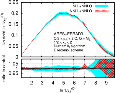
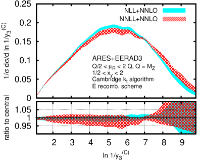
Figure 1: Differential distributions for the three-jet resolution in the Durham (left) and Cambridge (right) algorithms. The plots show both the NLL+NNLO (blue/solid) and the NNLL+NNLO (red/hatched) results.

In a similar way we approximate the original algorithm to compute the remaining NNLL corrections whose definition follows exactly the one given for event shapes Banfi:2014sua .

The considerations made so far for the Durham case can be straightforwardly adapted to any other rIRC jet algorithm. In particular, for the Cambridge algorithm the NNLL logarithmic structure is much simpler. In this case the ordering variable (2) only depends on the angular distance between emissions. Since at NLL all partons are well separated in rapidity, there will be no clustering between the emissions, and each of them will be recombined with one of the Born legs in an angular-ordered way. One therefore obtains the trivial result ${\cal F}_{\rm NLL}(\lambda)=1$. The same arguments imply that the NNLL corrections $\delta\mathcal{F}_{\rm sc}=\delta\mathcal{F}_{\rm hc}=0$ BMMZadditional . Moreover, both the recoil and the wide-angle corrections admit a simple analytic form given that the emission emitted either at wide angles or collinearly will never cluster with any of the other soft-collinear emissions. As a consequence the contribution from this emission factorizes with respect to the remaining ensemble BMMZadditional . The same property applies to the clustering and correlated corrections which can be entirely formulated in terms of the clustering condition between two soft-collinear emissions BMMZadditional , analogously to the jet veto resummation Banfi:2012jm . We note that the freezing condition present in the Cambridge algorithm does not play a role at NNLL. Therefore the AO version of the Durham algorithm coincides with the Cambridge algorithm at this order, while the two differ at NNLO.

We tested our results by subtracting the derivative of the second-order expansion of eq. (The two-jet rate in $e^{+}e^{-}$ at next-to-next-to-leading-logarithmic order) from the ${\cal O}(\alpha_{s}^{2})$ distributions obtained with the generator Event2 Catani:1996vz , finding agreement BMMZadditional . Moreover, we applied the method to both the inclusive-$k_{t}$ Weinzierl:2010cw ; Cacciari:2011ma and the flavor-$k_{t}$ Banfi:2006hf algorithms, finding also perfect agreement with Event2 at ${\cal O}(\alpha_{s}^{2})$.

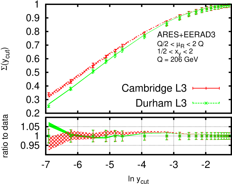
Figure 2: Comparison of NNLL+NNLO predictions for the two-jet rates to data from the L3 collaboration Achard:2004sv .

We illustrate the impact of our calculation by matching the NNLL two-jet rate (The two-jet rate in $e^{+}e^{-}$ at next-to-next-to-leading-logarithmic order) to the ${\cal O}(\alpha_{s}^{3})$ result obtained with the program EERAD3 Ridder:2014wza for both the Durham and the Cambridge algorithms. Figure 1 shows the matched differential distributions for the three-jet resolution parameter, defined in (3), at NNLL+NNLO and NLL+NNLO. The results are obtained at $Q=M_{Z}$, using the coupling $\alpha_{s}(M_{Z})=0.118$, and the $E$ recombination scheme. To impose unitarity, following ref. Banfi:2014sua , we employ the modified logarithms

$$\ln\frac{1}{y_{3}}\to\ln\left(1+\left(\frac{x_{y}}{y_{3}}\right)-\left(\frac{x_{y}}{y_{\rm 3,max}}\right)\right)\,,$$ (7)

in such a way that the $x_{y}$ dependence is N³LL. This also ensures that the distribution vanishes at the kinematical endpoint $y_{\rm 3,max}$, taken from the NNLO result. Furthermore, the variation of $x_{y}$ probes the size of subleading logarithmic effects. Our theoretical uncertainties are obtained by varying, one at the time, $x_{y}$ and the renormalization scale $\mu_{R}$ by a factor of two in either direction around the central values $x_{y}=1$ and $\mu_{R}=Q$, and taking the envelope of these variations.

For the Durham algorithm, as expected, we observe a significant reduction of the theory error when going from NLL to NNLL. On the contrary, for the Cambridge algorithm, NNLL corrections are quite large, and the NNLL uncertainty is larger than the NLL one, which in turn seems to be underestimated. This effect can be understood by observing that the NLL prediction for the Cambridge algorithm does not contain any information about multiple emissions effects since no clustering occurs at this order and ${\cal F}_{\rm NLL}=1$. These effects appear only at NNLL, explaining the sizable numerical corrections. It follows that the NLL theory uncertainty as estimated in figure 1 is unable to capture large subleading effects. A similar phenomenon was already observed in the resummation for the jet-veto efficiency Banfi:2012jm .

To conclude, in figure 2 we compare our NNLL+NNLO prediction to the data taken by the L3 collaboration at LEP2 Achard:2004sv at $Q=206$ GeV. At this high center-of-mass energy the impact of hadronization effects, which are not included in our calculation, is moderate. Overall, we find good agreement with data down to the lowest values of $y_{\rm cut}$. Owing to the small residual perturbative uncertainties, our calculation shows promise for a precise determination of the strong coupling using $e^{+}e^{-}$ data measured at LEP.

In this paper we have presented a general method for final-state resummation at NNLL order for global rIRC safe observables that vanish in the two-jet limit, where a single family of large logarithms is resummed. We derived explicit results for the two-jet rate in $e^{+}e^{-}$. The computer code ARES used to obtain the results presented here can be made available upon request to the authors.

Supplemental material

We provide here explicit formulae that complete the discussion of the letter. Furthermore analytic results for the case of the Cambridge algorithm are derived explicitly.

.1 Next-to-next-to-leading-logarithmic real corrections

.1.1 Resolved real corrections at NLL

At NLL accuracy the details of the resolved real radiation are described by the multiple emission function $\mathcal{F}_{\rm NLL}$. $\mathcal{F}_{\rm NLL}$ is defined on an ensemble of independently-emitted soft and collinear partons, widely separated in rapidity. Moreover, all emissions have the same rapidity bound $|\eta_{i}|<\ln(1/\sqrt{y_{\rm cut}})$. The multiple emission function depends on $\lambda=\alpha_{s}(\mu_{R})\beta_{0}\ln(1/y_{\rm cut})$ ($\mu_{R}$ being the renormalization scale) with $\beta_{0}=\frac{11C_{A}-2n_{f}}{12\pi}$, and is defined as

$$\mathcal{F}_{\rm NLL}(\lambda)=\int d{\cal Z}[\{R^{\prime}_{\mathrm{NLL},\ell_{i}},k_{i}\}]\,\Theta\left(1-\lim_{y_{\rm cut}\to 0}\frac{\overline{y}_{3}^{\rm sc}(\{\tilde{p}\},\{k_{i}\})}{y_{\rm cut}}\right)\,.$$ (8)

In the above equation, $d{\cal Z}[\{R^{\prime}_{\mathrm{NLL},\ell_{i}},k_{i}\}]$ is the soft-collinear measure, which is defined for any arbitrary function $G(\{\tilde{p}\},k_{1},\dots,k_{n})$ as

$$\begin{split}\int d{\cal Z}[\{R^{\prime}_{\mathrm{NLL},\ell_{i}},k_{i}\}]G(\{\tilde{p}\},\{k_{i}\})=\epsilon^{R^{\prime}_{\mathrm{NLL}}}\sum_{n=0}^{\infty}\frac{1}{n!}\prod_{i=1}^{n}\int_{\epsilon}^{\infty}\frac{d\zeta_{i}}{\zeta_{i}}\int_{0}^{2\pi}\frac{d\phi_{i}}{2\pi}\sum_{\ell_{i}=1,2}\int_{0}^{1}d\xi_{i}^{(\ell_{i})}\,R^{\prime}_{\mathrm{NLL},\ell_{i}}G(\{\tilde{p}\},k_{1},\dots,k_{n})\,.\end{split}$$ (9)

Here $\zeta_{i}=\frac{k_{ti}^{2}}{Q^{2}y_{\rm cut}}$, $\xi_{i}^{(\ell_{i})}=|\eta_{i}|/\eta_{\max}$, and $R^{\prime}_{\mathrm{NLL},\ell}$ is defined in appendix B of ref. Banfi:2014sua . For each emission $k_{i}$ the sum is over the two emitting legs $\ell_{i}=1,2$, and $\ell_{i}=1$ ($\ell_{i}=2$) when $\eta_{i}$ is positive (negative). The measure (9) differs from that used in the case of event shapes, because of the presence of the integrals over the rapidity fractions $\xi_{i}^{(\ell_{i})}$, where in this case $\eta_{\max}=\ln(1/\sqrt{y_{\rm cut}})$. In the case of event-shapes, one could integrate inclusively over the rapidity fractions. This is not the case for $y_{3}$ since it depends explicitly on the particles’ $\xi_{i}^{(\ell_{i})}$. $d{\cal Z}[\{R^{\prime}_{\mathrm{NLL},\ell_{i}},k_{i}\}]$ satisfies the normalization condition

$$\int d{\cal Z}[\{R^{\prime}_{\mathrm{NLL},\ell_{i}},k_{i}\}]\prod_{i}\Theta\left(1-\lim_{y_{\rm cut}\to 0}\frac{\overline{y}_{3}^{\rm sc}(\{\tilde{p}\},k_{i})}{y_{\rm cut}}\right)=1\,.$$ (10)

Note that in the presence of a single soft-collinear emission $\overline{y}_{3}^{\rm sc}(\{\tilde{p}\},k_{i})=y_{3}^{\rm sc}(\{\tilde{p}\},k_{i})$.

• Durham algorithm: when emissions are both soft and collinear, and strongly ordered in rapidity, the observable, denoted by $\overline{y}_{3}^{\rm sc}(\{\tilde{p}\},k_{1},\dots,k_{n})$, can be computed with the following simplified algorithm:

  • Find the index $I$ of the smallest $\overline{y}_{3}^{\rm sc}(\{\tilde{p}\},k_{I})=y_{3}^{\rm sc}(\{\tilde{p}\},k_{I})=(k_{tI}/Q)^{2}$.

  • Considering only pseudo-particles $k_{j}$ collinear to the same leg $\ell$ as $I$, find parton $k_{J}$ which satisfies $\vec{k}_{tJ}\cdot\vec{k}_{tI}>0$ and has the smallest positive value of $\xi_{J}^{(\ell)}-\xi_{I}^{(\ell)}$.

  • If $k_{J}$ is found, recombine partons $I$ and $J$ into a new pseudo-particle $k_{P}$ with $\vec{k}_{tP}=\vec{k}_{tI}+\vec{k}_{tJ}$ and $\xi_{P}^{(\ell)}=\xi_{J}^{(\ell)}$. Otherwise, $k_{I}$ is clustered with a Born leg, and removed from the list of pseudo-particles.

  • If only one pseudo-particle $k_{P}$ remains, then $\overline{y}_{3}^{\rm sc}(\{\tilde{p}\},k_{1},\dots,k_{n})=(k_{tP}/Q)^{2}$, otherwise go back to step 1.

• Cambridge algorithm: since for the Cambridge algorithm no recombinations occur if all emissions are widely separated in rapidity, we have:

  $$\Theta\left(1-\lim_{y_{\rm cut}\to 0}\frac{\overline{y}_{3}^{\rm sc}(\{\tilde{p}\},k_{1},\dots,k_{n})}{y_{\rm cut}}\right)=\prod_{i=1}^{n}\Theta\left(1-\lim_{y_{\rm cut}\to 0}\frac{y_{3}^{\rm sc}(\{\tilde{p}\},k_{i})}{y_{\rm cut}}\right)\,.$$ (11)

  Therefore, for this algorithm, $\mathcal{F}_{\rm NLL}(\lambda)=1$.

.1.2 Soft-collinear correction

The soft-collinear NNLL correction takes into account the correct rapidity bound for one of the soft-collinear emissions that give rise to the NLL multiple emission function, as well as NNLL contributions arising from the running of the QCD coupling in the soft-collinear matrix elements. We denote by $k$ the emission for which we account for either effect, and introduce $\zeta$ such that $y_{3}^{\rm sc}(\{\tilde{p}\},k)=k_{t}^{2}/Q^{2}=\zeta y_{\rm cut}$. If $y_{3}$ were an event shape, we could integrate inclusively over the rapidity fraction of each emission. As a result, the emission probability for $k$, collinear to the Born leg $\ell$, would be proportional to the function $R^{\prime}_{\ell}\left(\zeta y_{\rm cut}\right)$ defined in Section 2 of ref. Banfi:2014sua . In this case both NNLL effects could be accounted for by expanding $R^{\prime}_{\ell}\left(\zeta y_{\rm cut}\right)$ as follows:

$$R^{\prime}_{\ell}\left(\zeta y_{\rm cut}\right)\simeq R^{\prime}_{\rm NLL,\ell}(y_{\rm cut})+\delta R^{\prime}_{\rm NNLL,\ell}(y_{\rm cut})+R^{\prime\prime}_{\ell}(y_{\rm cut})\ln\frac{1}{\zeta}\,.$$ (12)

The full expressions for $\delta R^{\prime}_{\rm NNLL,\ell}(y_{\rm cut})$ and $R^{\prime\prime}_{\ell}(y_{\rm cut})$ are given in ref. Banfi:2014sua . In the present case, this correction must be formulated in a slightly more general way than the corresponding one defined for event-shape observables Banfi:2014sua . The NNLL term proportional to $\delta R^{\prime}_{\rm NNLL,\ell}(y_{\rm cut})$ in eq. (12) contains the contribution from the one-loop cusp anomalous dimension as well as from the two-loop running of the QCD coupling. In this term, the rapidity of all emissions is bounded by the NLL limit $\ln(1/\sqrt{y_{\rm cut}})$. Therefore this correction is unchanged with respect to event shapes, and gives rise to

$$\begin{split}&\frac{\pi}{\alpha_{s}(\mu_{R})}\int_{0}^{\infty}\frac{d\zeta}{\zeta}\int_{0}^{2\pi}\frac{d\phi}{2\pi}\sum_{\ell=1,2}\int_{0}^{1}d\xi^{(\ell)}\delta R^{\prime}_{{\rm NNLL},\ell}\int d{\cal Z}[\{R^{\prime}_{\mathrm{NLL},\ell_{i}},k_{i}\}]\times\\ &\times\left[\Theta\left(1-\lim_{y_{\rm cut}\to 0}\frac{\overline{y}_{3}^{\rm sc}(\{\tilde{p}\},k,\{k_{i}\})}{y_{\rm cut}}\right)-\Theta(1-\zeta)\Theta\left(1-\lim_{y_{\rm cut}\to 0}\frac{\overline{y}_{3}^{\rm sc}(\{\tilde{p}\},\{k_{i}\})}{y_{\rm cut}}\right)\right]\,,\end{split}$$ (13)

where the soft-collinear observable $\overline{y}_{3}^{\rm sc}(\{\tilde{p}\},k,\{k_{i}\})$ is computed by means of the NLL algorithms given in the previous section.

The remaining term in the r.h.s. of eq. (12) is proportional to the function $R^{\prime\prime}_{\ell}(y_{\rm cut})$ given by

$$R^{\prime\prime}_{\ell}(y_{\rm cut})=\frac{\alpha_{s}(\sqrt{y_{\rm cut}}Q)}{2\pi}C_{F}\left(\beta_{0}\alpha_{s}(\sqrt{y_{\rm cut}}Q)\ln\left(\frac{1}{y_{\rm cut}}\right)+1\right)\,.$$ (14)

The above function is made of two contributions: the term proportional to $\beta_{0}$ arises from expanding $\alpha_{s}(k_{t})$ around $\alpha_{s}(\sqrt{y_{\rm cut}}Q)$ in the soft emission matrix element as follows

$$\alpha_{s}(k_{t})\simeq\alpha_{s}(\sqrt{y_{\rm cut}}Q)+\beta_{0}\alpha_{s}^{2}(\sqrt{y_{\rm cut}}Q)\ln\frac{1}{\zeta}\,.$$ (15)

The term proportional to $\ln(1/\zeta)$ is purely NNLL. Therefore, when integrating over the emissions’ phase space, we can set all rapidity bounds to the NLL limit $\ln(1/\sqrt{y_{\rm cut}})$, neglecting subleading logarithmic terms. This approximation is identical to the one defining eq. (13), therefore the two corrections can be put together to define the running-coupling part $\delta\mathcal{F}_{\rm sc}^{\rm\,rc}$ of the soft-collinear correction as follows:

$$\begin{split}\delta\mathcal{F}_{\rm sc}^{\rm\,rc}(\lambda)&=\frac{\pi}{\alpha_{s}(\mu_{R})}\int_{0}^{\infty}\frac{d\zeta}{\zeta}\int_{0}^{2\pi}\frac{d\phi}{2\pi}\sum_{\ell=1,2}\int_{0}^{1}d\xi^{(\ell)}\left(\delta R^{\prime}_{{\rm NNLL},\ell}+\lambda R^{\prime\prime}_{\ell}\ln\frac{1}{\zeta}\right)\int d{\cal Z}[\{R^{\prime}_{\mathrm{NLL},\ell_{i}},k_{i}\}]\times\\ &\times\left[\Theta\left(1-\lim_{y_{\rm cut}\to 0}\frac{\overline{y}_{3}^{\rm sc}(\{\tilde{p}\},k,\{k_{i}\})}{y_{\rm cut}}\right)-\Theta(1-\zeta)\Theta\left(1-\lim_{y_{\rm cut}\to 0}\frac{\overline{y}_{3}^{\rm sc}(\{\tilde{p}\},\{k_{i}\})}{y_{\rm cut}}\right)\right]\,,\end{split}$$ (16)

where

$$\lambda R^{\prime\prime}_{\ell}=\frac{C_{F}}{2\pi}\beta_{0}\alpha_{s}^{2}(\sqrt{y_{\rm cut}}Q)\ln\frac{1}{y_{\rm cut}}\,.$$ (17)

The second term in eq. (14) is associated with the correct rapidity bound for emission $k$. Given that the observable in this case depends on the rapidity fractions of the emissions, unlike for event shapes the latter correction is not accounted for by eq. (12).

To study how the form of this correction is modified, let us consider a given ensemble of $n$ emissions $k_{1},\dots,k_{n}$ strongly ordered in rapidity, collinear to the same hard leg, say $\ell=1$ which corresponds to positive rapidities. All of the emissions have the NLL rapidity bound $\ln(1/\sqrt{y_{\rm cut}})$ except for the emission $k_{j}$ which has the exact rapidity bound $\ln(Q/k_{tj})>\ln(1/\sqrt{y_{\rm cut}})$. The latter relation can be proven by observing that for all emissions $k_{i}$ one has that $k_{ti}\leq\sqrt{y_{\rm cut}}Q$. This statement is trivial if no clustering occurs. If pseudo-particles $k_{I}$ and $k_{J}$ are recombined, the transverse momentum of the resulting jet $|\vec{k}_{tI}+\vec{k}_{tJ}|$ will be larger than $k_{tI}$ and $k_{tJ}$. This is because a clustering occurs only if $\vec{k}_{tI}\cdot\vec{k}_{tJ}>0$ in the NLL algorithm. By induction, in all configurations which end up with two jets (i.e. $\overline{y}_{3}^{\rm sc}(\{\tilde{p}\},\{k_{i}\})<y_{\rm cut}$), one has $k_{ti}\leq\sqrt{y_{\rm cut}}Q$ for all particles $k_{i}$.

Let us consider a given ordering of transverse momenta $\{k_{ti}\}$ of the $n$ emissions. For such a configuration of transverse momenta, $n!$ rapidity orderings are available. Each rapidity ordering corresponds to a different value for the observable in its NLL version (see the algorithm given in the previous section). We now assume that all emissions but $k_{j}$ have the NLL rapidity bound $\ln(1/\sqrt{y_{\rm cut}})$, whereas $\eta_{j}<\ln(Q/k_{tj})$. Without loss of generality, we start by considering the generic ordering $\eta_{1}>\eta_{2}>\dots>\eta_{j}>\dots>\eta_{n}$. We can identify two possible scenarios: when the most forward emission has rapidity $\eta_{1}<\ln(1/\sqrt{y_{\rm cut}})$, and when $\ln(1/\sqrt{y_{\rm cut}})<\eta_{1}<\ln(Q/k_{t1})$. In the first case, after including running couplings and color factors, the corresponding rapidity integral is

$$I_{1}^{(n)}= \left(\frac{C_{F}}{\pi}\right)^{n}\prod_{i=1}^{n}\alpha_{s}(k_{ti})\int^{\ln(1/\sqrt{y_{\rm cut}})}d\eta_{1}\int^{\eta_{1}}d\eta_{2}\dots\int^{\eta_{j-1}}\!\!d\eta_{j}\dots\int^{\eta_{n-1}}\!\!d\eta_{n}=\left(\frac{C_{F}}{\pi}\right)^{n}\prod_{i=1}^{n}\alpha_{s}(k_{ti})\frac{1}{n!}\ln^{n}\frac{1}{\sqrt{y_{\rm cut}}}\,.$$ (18)

We stress that this result is the same regardless of the rapidity bound of emissions $k_{2},\cdots,k_{n}$. Note that the integral in eq. (18) is correct under the assumption of strong rapidity ordering. The extra NNLL correction originating from configurations in which two emissions are close in rapidity, for which the NLL version of the observable cannot be applied, is taken into account in the clustering corrections derived below. It is manifest that the integral (18) contributes to a given kinematic configuration starting at NLL. To neglect subleading effects, we can expand the strong coupling in eq. (18) as in eq. (15). This leads to

$$I_{1}^{(n)} =\left(\frac{C_{F}}{\pi}\right)^{n}\alpha_{s}^{n}(\sqrt{y_{\rm cut}}Q)\frac{1}{n!}\ln^{n}\frac{1}{\sqrt{y_{\rm cut}}}+\beta_{0}\alpha_{s}^{n+1}(\sqrt{y_{\rm cut}}Q)\left(\frac{C_{F}}{\pi}\right)^{n}\frac{1}{n!}\ln^{n}\frac{1}{\sqrt{y_{\rm cut}}}\sum_{i=1}^{n}\ln\frac{1}{\zeta_{i}}+{\cal O}({\rm N^{3}LL})$$

$$\simeq\frac{(R^{\prime}_{\ell}(y_{\rm cut}))^{n}}{n!}+\lambda R^{\prime\prime}_{\ell}(y_{\rm cut})\frac{(R^{\prime}_{\ell}(y_{\rm cut}))^{n-1}}{n!}\sum_{i=1}^{n}\ln\frac{1}{\zeta_{i}}\,,$$ (19)

where we used

$$\ln\frac{Q}{k_{ti}}=\ln\frac{1}{\sqrt{y_{\rm cut}}}+\ln\frac{1}{\sqrt{\zeta_{i}}}\,,$$ (20)

and $\zeta_{i}=(k_{ti}/Q)^{2}/y_{\rm cut}$.

Analogously, the configurations in which $\ln(1/\sqrt{y_{\rm cut}})<\eta_{1}<\ln(Q/k_{t1})$ lead to

$$I_{2}^{(n)}=\left(\frac{C_{F}}{\pi}\right)^{n}\prod_{i=1}^{n}\alpha_{s}(k_{ti})\int^{\ln(Q/k_{t1})}_{\ln(1/\sqrt{y_{\rm cut}})}d\eta_{1}\int^{\eta_{1}}d\eta_{2}\dots\int^{\eta_{j-1}}\!\!d\eta_{j}\dots\int^{\eta_{n-1}}\!\!d\eta_{n}\,.$$ (21)

The bound in $\eta_{2}$ can be replaced with $\ln(1/\sqrt{y_{\rm cut}})$ since the region where $\eta_{2}>\ln(1/\sqrt{y_{\rm cut}})$ gives rise to a subleading correction. Moreover, the argument of the running coupling can be replaced with $\sqrt{y_{\rm cut}}Q$ for all emissions at NNLL. With these replacements we have

$$I_{2}^{(n)}=\left(\frac{C_{F}}{\pi}\right)^{n}\alpha_{s}^{n}(Q\sqrt{y_{\rm cut}})\frac{1}{(n-1)!}\ln^{n-1}\frac{1}{\sqrt{y_{\rm cut}}}\ln\frac{1}{\sqrt{\zeta_{1}}}=(1-\lambda)R^{\prime\prime}_{\ell}(y_{\rm cut})\frac{(R^{\prime}_{\ell}(y_{\rm cut}))^{n-1}}{(n-1)!}\ln\frac{1}{\zeta_{1}}\,.$$ (22)

Eq. (22) gives a pure NNLL contribution, and it is obtained in the limit of strong rapidity ordering. The configuration in which two emissions are close in rapidity here gives a subleading correction, proving that there is no overlap with the configurations contributing to the clustering correction.

In eq. (.1.2) we can recognise the NLL contribution (first term in the r.h.s.) that gives rise to the function ${\cal F}_{\rm NLL}$, and the NNLL correction proportional to $\lambda R^{\prime\prime}_{\ell}$ in eq. (16), that starts at ${\cal O}(\alpha_{s}^{3})$. Eq. (22) gives rise to a pure NNLL correction which accounts for the exact rapidity bound for a single emission. At NNLL accuracy, this bound matters only for the most forward/backward emission. We denote this correction by $\delta\mathcal{F}_{\rm sc}^{\rm\,rap}$.

In order to compute the latter to all orders, we set emission $k$, the one with the correct bound, to be the most forward/backward, and we generate randomly the rapidity fractions of the remaining emissions. This gives the following correction

$$\begin{split}\delta\mathcal{F}_{\rm sc}^{\rm\,rap}(\lambda)&=\frac{\pi}{\alpha_{s}(\mu_{R})}\int_{0}^{\infty}\frac{d\zeta}{\zeta}\int_{0}^{2\pi}\frac{d\phi}{2\pi}\sum_{\ell=1,2}(1-\lambda)R^{\prime}_{\ell}\ln\frac{1}{\zeta}\int d{\cal Z}[\{R^{\prime}_{\mathrm{NLL},\ell_{i}},k_{i}\}]\times\\ &\times\left[\Theta\left(1-\lim_{y_{\rm cut}\to 0}\frac{\overline{y}_{3}^{\rm sc}(\{\tilde{p}\},k,\{k_{i}\})}{y_{\rm cut}}\right)-\Theta(1-\zeta)\Theta\left(1-\lim_{y_{\rm cut}\to 0}\frac{\overline{y}_{3}^{\rm sc}(\{\tilde{p}\},\{k_{i}\})}{y_{\rm cut}}\right)\right]_{\xi^{(\ell)}=1}\,,\end{split}$$ (23)

where now $\zeta,\xi^{(\ell)},\phi$ refer to the emission $k$ with exact rapidity bound, and $(1-\lambda)R^{\prime\prime}_{\ell}=C_{F}\alpha_{s}(\sqrt{y_{\rm cut}}Q)/(2\pi)$ Banfi:2014sua . The condition $\xi^{(\ell)}=1$ indicates the rapidity fraction of $k$ has been fixed to $1$ reflecting the fact that the emission with the correct rapidity bound must be the most forward/backward in rapidity.

In the case of the event shapes, the integrals over the rapidity fractions can be evaluated inclusively, and the sum

$$\delta\mathcal{F}_{\rm sc}^{\rm\,rc}(\lambda)+\delta\mathcal{F}_{\rm sc}^{\rm\,rap}(\lambda)$$ (24)

reproduces the soft-collinear correction formulated in ref. Banfi:2014sua . Therefore, the formulation given here can be easily adapted to other observables, including event shapes.

• Cambridge algorithm: the form of the soft-collinear corrections $\delta\mathcal{F}_{\rm sc}$ can be simplified using eq. (11) as

  $$\Theta\left(1-\lim_{y_{\rm cut}\to 0}\frac{\overline{y}_{3}^{\rm sc}(\{\tilde{p}\},k,\{k_{i}\})}{y_{\rm cut}}\right)-\Theta(1-\zeta)\Theta\left(1-\lim_{y_{\rm cut}\to 0}\frac{\overline{y}_{3}^{\rm sc}(\{\tilde{p}\},\{k_{i}\})}{y_{\rm cut}}\right)$$

  $$=\left[\Theta\left(1-\lim_{y_{\rm cut}\to 0}\frac{\overline{y}_{3}^{\rm sc}(\{\tilde{p}\},k)}{y_{\rm cut}}\right)-\Theta(1-\zeta)\right]\prod_{i=1}^{n}\Theta\left(1-\lim_{y_{\rm cut}\to 0}\frac{y_{3}^{\rm sc}(\{\tilde{p}\},k_{i})}{y_{\rm cut}}\right)=0\,,$$ (25)

  where we made use of the definition of $\zeta=y_{3}^{\rm sc}(\{\tilde{p}\},\{k\})=\zeta y_{\rm cut}$. This result trivially leads to $\delta\mathcal{F}_{\rm sc}(\lambda)=0$ for the Cambridge algorithm.

.1.3 Clustering corrections

This correction describes an ensemble of soft-collinear partons emitted off the Born legs of which at most two are close in rapidity and the remaining ones are strongly separated in angle. For rIRC safe observables, this kinematical configuration contributes only at NNLL order and beyond. The clustering correction $\delta\mathcal{F}_{\rm clust}$ encodes the abelian contribution to the above configuration, where the two partons which are close in rapidity have been emitted independently. Its expression reads

$$\begin{split}\delta\mathcal{F}_{\rm clust}(\lambda)&=\frac{1}{2!}\int_{0}^{\infty}\frac{d\zeta_{a}}{\zeta_{a}}\int_{0}^{2\pi}\frac{d\phi_{a}}{2\pi}\sum_{\ell_{a}=1,2}\int_{0}^{1}d\xi_{a}^{(\ell_{a})}\left(\frac{2C_{F}\lambda}{\beta_{0}}\frac{R^{{}^{\prime\prime}}_{\ell_{a}}(y_{\rm cut})}{\alpha_{s}(\mu_{R})}\right)\int_{0}^{\infty}\frac{d\kappa}{\kappa}\int_{-\infty}^{\infty}\!\!\!d\eta\int_{0}^{2\pi}\frac{d\phi}{2\pi}\times\\ &\times\int d{\cal Z}[\{R^{\prime}_{\mathrm{NLL},\ell_{i}},k_{i}\}]\left[\Theta\left(1-\lim_{y_{\rm cut}\to 0}\frac{y_{3}^{\rm sc}(\{\tilde{p}\},k_{a},k_{b},\{k_{i}\})}{y_{\rm cut}}\right)-\Theta\left(1-\lim_{y_{\rm cut}\to 0}\frac{\overline{y}_{3}^{\rm sc}(\{\tilde{p}\},k_{a},k_{b},\{k_{i}\})}{y_{\rm cut}}\right)\right]\,,\end{split}$$ (26)

where $y_{3}^{\rm sc}(\{\tilde{p}\},k_{a},k_{b},\{k_{i}\})$ is obtained with the clustering procedures outlined below for this type of kinematical configuration, while $\overline{y}_{3}^{\rm sc}(\{\tilde{p}\},k_{a},k_{b},\{k_{i}\})$ is the NLL version of the algorithm. We have parameterized the phase space of the emission $k_{b}$ in terms of the variables

$$\kappa=k_{t,b}/k_{t,a}\,\qquad\eta=\eta_{b}-\eta_{a}\,,\qquad\phi=\phi_{b}-\phi_{a}\,.$$ (27)

In terms of these variables $k_{b}$ can be written as

$$k_{b}=\kappa\,Q\,\sqrt{\zeta_{a}y_{\rm cut}}(\cosh(\eta_{a}+\eta),\cos(\phi_{a}+\phi),\sin(\phi_{a}+\phi),\sinh(\eta_{a}+\eta))\,.$$ (28)

In order to eliminate subleading effects, in the calculation of the observable we impose that $k_{b}$ belongs to the same hemisphere as $k_{a}$. In practice, this is accomplished by setting $\ell_{b}=\ell_{a}$ and $\xi_{b}^{(\ell_{a})}=\xi_{a}^{(\ell_{a})}+\mathrm{sign}(\eta)\delta\xi$, with $\delta\xi$ an arbitrarily small quantity. Unlike for the jet rates, event shapes are independent of the rapidity fractions of the emissions, therefore this correction is absent for such observables.

• Durham algorithm: the resulting algorithm goes along the lines of the strongly-ordered one, with an additional condition to be checked after step 1.

  • Let $k_{J_{a}}$ and $k_{J_{b}}$ be the pseudo-particles containing the partons $k_{a}$ and $k_{b}$. If the latter pseudo-particles are close in rapidity (i.e. if neither $k_{a}$ nor $k_{b}$ have been recombined with a pseudo-particle with larger $\xi^{(\ell)}$), check whether $k_{J_{a}}$ and $k_{J_{b}}$ cluster, i.e. if

    $$\min\{E_{J_{a}},E_{J_{b}}\}^{2}|\vec{\theta}_{J_{a}}-\vec{\theta}_{J_{b}}|^{2}<\min\{k_{tJ_{a}},k_{tJ_{b}}\}^{2}\,$$ (29)

    is satisfied, where $\vec{\theta}_{i}=\vec{k}_{ti}/E_{i}$. If so, recombine $k_{J_{a}}$ and $k_{J_{b}}$ by adding transverse momenta vectorially, and setting the rapidity fraction of the resulting pseudo-particle $k_{J}$ to $\xi_{J}^{(\ell)}\simeq\xi_{J_{a}}^{(\ell)}\simeq\xi_{J_{b}}^{(\ell)}$.

  We denote by $y_{3}^{\rm sc}(\{\tilde{p}\},k_{1},\dots,k_{n})$ the resulting value of $y_{3}$, to distinguish it from $\overline{y}_{3}^{\rm sc}(\{\tilde{p}\},k_{1},\dots,k_{n})$ used to compute $\mathcal{F}_{\rm NLL}$. Both algorithms have to be employed to compute the functions $\delta\mathcal{F}_{\rm clust}$ and $\delta\mathcal{F}_{\rm correl}$.

• Cambridge algorithm: in the case of the Cambridge algorithm, no recombination occurs whenever emissions are widely separated in angle. Therefore the clustering correction simply reduces to a clustering of two independently-emitted soft-collinear partons. In eq. (26), one can make the usual replacement

  $$\Theta\left(1-\lim_{y_{\rm cut}\to 0}\frac{y_{3}^{\rm sc}(\{\tilde{p}\},k_{a},k_{b},k_{1},\dots,k_{n})}{y_{\rm cut}}\right)=\Theta\left(1-\lim_{y_{\rm cut}\to 0}\frac{y_{3}^{\rm sc}(\{\tilde{p}\},k_{a},k_{b})}{y_{\rm cut}}\right)\prod_{i=1}^{n}\Theta\left(1-\lim_{y_{\rm cut}\to 0}\frac{y_{3}^{\rm sc}(\{\tilde{p}\},k_{i})}{y_{\rm cut}}\right)\,,$$ (30)

  and observe that the contribution of any number of widely separated emissions gives one, due to the normalization property of the measure $d{\cal Z}[\{R^{\prime}_{\mathrm{NLL},\ell_{i}},k_{i}\}]$ (10). As a consequence, the expression in eq. (26) simplifies to

  $$\begin{split}\delta\mathcal{F}_{\rm clust}(\lambda)&=\frac{1}{2!}\int_{0}^{\infty}\frac{d\zeta_{a}}{\zeta_{a}}\int_{0}^{2\pi}\frac{d\phi_{a}}{2\pi}\sum_{\ell_{a}=1,2}\int_{0}^{1}d\xi_{a}^{(\ell_{a})}\left(\frac{2C_{F}\lambda}{\beta_{0}}\frac{R^{{}^{\prime\prime}}_{\ell_{a}}(y_{\rm cut})}{\alpha_{s}(\mu_{R})}\right)\int_{0}^{\infty}\frac{d\kappa}{\kappa}\int_{-\infty}^{\infty}\!\!\!d\eta\int_{0}^{2\pi}\frac{d\phi}{2\pi}\times\\ &\times\left[\Theta\left(1-\lim_{y_{\rm cut}\to 0}\frac{y_{3}^{\rm sc}(\{\tilde{p}\},k_{a},k_{b})}{y_{\rm cut}}\right)-\Theta\left(1-\lim_{y_{\rm cut}\to 0}\frac{\overline{y}_{3}^{\rm sc}(\{\tilde{p}\},k_{a},k_{b})}{y_{\rm cut}}\right)\right]\,,\end{split}$$ (31)

  which is non-zero only if the two emissions are clustered by the NNLL algorithm, yielding

  $$\begin{split}\delta\mathcal{F}_{\rm clust}(\lambda)&=\frac{1}{2!}\int_{0}^{\infty}\frac{d\zeta_{a}}{\zeta_{a}}\int_{0}^{2\pi}\frac{d\phi_{a}}{2\pi}\sum_{\ell_{a}=1,2}\int_{0}^{1}d\xi_{a}^{(\ell_{a})}\left(\frac{2C_{F}\lambda}{\beta_{0}}\frac{R^{{}^{\prime\prime}}_{\ell_{a}}(y_{\rm cut})}{\alpha_{s}(\mu_{R})}\right)\int_{0}^{\infty}\frac{d\kappa}{\kappa}\int_{-\infty}^{\infty}\!\!\!d\eta\int_{0}^{2\pi}\frac{d\phi}{2\pi}\times\\ &\times\left[\Theta\left(1-\lim_{y_{\rm cut}\to 0}\frac{y_{3}^{\rm sc}(\{\tilde{p}\},k_{a}+k_{b})}{y_{\rm cut}}\right)-\Theta\left(1-\lim_{y_{\rm cut}\to 0}\frac{\max(y_{3}^{\rm sc}(\{\tilde{p}\},k_{a}),y_{3}^{\rm sc}(\{\tilde{p}\},k_{b}))}{y_{\rm cut}}\right)\right]\Theta_{\rm clust}\,,\end{split}$$ (32)

  where $\Theta_{\rm clust}$ restricts the allowed phase space to the region where the two emissions $k_{a}$ and $k_{b}$ cluster. Using the ordering variable for the Cambridge algorithm (eq. (2)) in the small-angle approximation, emissions $a$ and $b$ will cluster if

  $$\begin{split}|\vec{\theta_{a}}-\vec{\theta_{b}}|^{2}&<\min\left\{\theta_{a},\theta_{b}\right\}^{2}\qquad\Leftrightarrow\qquad\Theta_{\rm clust}=\Theta\left(\ln(2\cos\phi)-|\eta|\right)\Theta\left(\frac{\pi}{3}-|\phi|\right)\,.\end{split}$$ (33)

  Applying these constraints gives

  $$\begin{split}\delta\mathcal{F}_{\rm clust}(\lambda)&=\sum_{\ell_{a}=1,2}\left(\frac{2C_{F}\lambda}{\beta_{0}}\frac{R^{{}^{\prime\prime}}_{\ell_{a}}(y_{\rm cut})}{\alpha_{s}(\mu_{R})}\right)\int_{0}^{\infty}\frac{d\kappa}{\kappa}\int_{-\frac{\pi}{3}}^{\frac{\pi}{3}}\frac{d\phi}{2\pi}\ln(2\cos\phi)\ln\left(\frac{\max\left\{1,\kappa^{2}\right\}}{1+\kappa^{2}+2\kappa\cos\phi}\right)\\ &\approx\sum_{\ell_{a}=1,2}\left(\frac{2C_{F}\lambda}{\beta_{0}}\frac{R^{{}^{\prime\prime}}_{\ell_{a}}(y_{\rm cut})}{\alpha_{s}(\mu_{R})}\right)(-0.493943)\,.\end{split}$$ (34)

.1.4 Correlated corrections

The correlated correction describes an ensemble of independently-emitted soft-collinear partons of which one branches into either a quark or a gluon pair, denoted by $k_{a}$ and $k_{b}$. The property of rIRC safety ensures that the splitting can be treated inclusively at NLL, and at this order it contributes to the Sudakov radiator Banfi:2014sua . At NNLL the splitting must be resolved, and this is taken into account by correcting the inclusive approximation. This leads to

$$\begin{split}\delta\mathcal{F}_{\rm correl}(\lambda)&=\int_{0}^{\infty}\frac{d\zeta_{a}}{\zeta_{a}}\int_{0}^{2\pi}\frac{d\phi_{a}}{2\pi}\sum_{\ell_{a}=1,2}\int_{0}^{1}d\xi_{a}^{(\ell_{a})}\left(\frac{2C_{F}\lambda}{\beta_{0}}\frac{R^{{}^{\prime\prime}}_{\ell_{a}}(y_{\rm cut})}{\alpha_{s}(\mu_{R})}\right)\int_{0}^{\infty}\frac{d\kappa}{\kappa}\int_{-\infty}^{\infty}\!\!\!d\eta\int_{0}^{2\pi}\frac{d\phi}{2\pi}\frac{1}{2!}C_{ab}(\kappa,\eta,\phi)\times\\ &\times\int d{\cal Z}[\{R^{\prime}_{\mathrm{NLL},\ell_{i}},k_{i}\}]\left[\Theta\left(1-\lim_{y_{\rm cut}\to 0}\frac{y_{3}^{\rm sc}(\{\tilde{p}\},k_{a},k_{b},\{k_{i}\})}{y_{\rm cut}}\right)-\Theta\left(1-\lim_{y_{\rm cut}\to 0}\frac{\overline{y}_{3}^{\rm sc}(\{\tilde{p}\},k_{a}+k_{b},\{k_{i}\})}{y_{\rm cut}}\right)\right]\,,\end{split}$$ (35)

where

$$C_{ab}(\kappa,\eta,\phi)=\frac{\tilde{M}^{2}(k_{a},k_{b})}{M_{sc}^{2}(k_{a})M_{sc}^{2}(k_{b})}\,,$$ (36)

is the ratio of the correlated soft matrix element $\tilde{M}^{2}(k_{a},k_{b})=M^{2}(k_{a},k_{b})-M^{2}(k_{a})M^{2}(k_{b})$ (i.e. the difference between the full two-parton matrix element in the soft limit and the independent emission contribution) to the product of the two independent soft-collinear matrix elements for the emissions $k_{a}$ and $k_{b}$. Notice that $C_{ab}$ depends only on the correlation variables $\kappa,\eta,\phi$ defined in eq. (27). The observable $y_{3}^{\rm sc}(\{\tilde{p}\},k_{a},k_{b},\{k_{i}\})$ is computed with the same algorithm used for the clustering correction. In the inclusive approximation $y_{3}^{\rm sc}(\{\tilde{p}\},k_{a}+k_{b},\{k_{i}\})$ reduces to the NLL value $\overline{y}_{3}^{\rm sc}(\{\tilde{p}\},k_{a}+k_{b},\{k_{i}\})$. As done for the clustering correction, we impose that $k_{b}$ belongs to the same hemisphere as $k_{a}$ in order to neglect undesired subleading effects. While for the Durham the observable $y_{3}^{\rm sc}(\{\tilde{p}\},k_{a},k_{b},\{k_{i}\})$ is computed using the algorithm given above for the clustering corrections, in the case of the Cambridge the final expression simplifies considerably.

• Cambridge algorithm: in the case of the Cambridge algorithm we can integrate out the harmless rapidity-separated soft-collinear ensemble and write

  $$\begin{split}\delta\mathcal{F}_{\rm correl}(\lambda)&=\int_{0}^{\infty}\frac{d\zeta_{a}}{\zeta_{a}}\int_{0}^{2\pi}\frac{d\phi_{a}}{2\pi}\sum_{\ell_{a}=1,2}\int_{0}^{1}d\xi_{a}^{(\ell_{a})}\left(\frac{2C_{F}\lambda}{\beta_{0}}\frac{R^{{}^{\prime\prime}}_{\ell_{a}}(y_{\rm cut})}{\alpha_{s}(\mu_{R})}\right)\int_{0}^{\infty}\frac{d\kappa}{\kappa}\int_{-\infty}^{\infty}\!\!\!d\eta\int_{0}^{2\pi}\frac{d\phi}{2\pi}\frac{1}{2!}C_{ab}(\kappa,\eta,\phi)\times\\ &\times\left[\Theta\left(1-\lim_{y_{\rm cut}\to 0}\frac{\max\left\{y_{3}^{\rm sc}(\{\tilde{p}\},k_{a}),y_{3}^{\rm sc}(\{\tilde{p}\},k_{b})\right\}}{y_{\rm cut}}\right)-\Theta\left(1-\lim_{y_{\rm cut}\to 0}\frac{y_{3}^{\rm sc}(\{\tilde{p}\},k_{a}+k_{b})}{y_{\rm cut}}\right)\right](1-\Theta_{\rm clust})\,,\end{split}$$ (37)

  where $\Theta_{\rm clust}$ is defined in eq. (33). It is clear in fact that $\delta\cal{F}_{\rm correl}$ is non-zero only when $k_{a}$ and $k_{b}$ are not clustered in the first $\Theta$ function. This leads to

  $$\begin{split}\delta\mathcal{F}_{\rm correl}(\lambda)&=\sum_{\ell_{a}=1,2}\left(\frac{2C_{F}\lambda}{\beta_{0}}\frac{R^{{}^{\prime\prime}}_{\ell_{a}}(y_{\rm cut})}{\alpha_{s}(\mu_{R})}\right)\int_{0}^{\infty}\frac{d\kappa}{\kappa}\int_{0}^{2\pi}\frac{d\phi}{2\pi}\frac{1}{2!}\int_{-\infty}^{\infty}\!\!\!d\eta\,C_{ab}(\kappa,\eta,\phi)\ln\left(\frac{1+\kappa^{2}+2\kappa\cos\phi}{\max\left\{1,\kappa^{2}\right\}}\right)(1-\Theta_{\rm clust})\,.\\ \end{split}$$ (38)

  This integral can be evaluated numerically giving

  $$\begin{split}\delta\mathcal{F}_{\rm correl}(\lambda)&\approx\sum_{\ell_{a}=1,2}\left(\frac{\lambda}{\beta_{0}}\frac{R^{{}^{\prime\prime}}_{\ell_{a}}(y_{\rm cut})}{\alpha_{s}(\mu_{R})}\right)(2.1011(2)C_{A}+1.496(1)\times 10^{-2}n_{f})\,,\end{split}$$ (39)

  where the number in round brackets is the uncertainty in the last digit.

.1.5 Hard-collinear and recoil corrections

The hard-collinear and recoil corrections describe configurations in which a parton of the ensemble is emitted collinearly to one of the Born legs and carries a significant fraction $z$ of the emitter’s momentum.

The hard-collinear correction takes into account the exact matrix element for this hard-collinear emission:

$$\begin{split}&\delta\mathcal{F}_{\rm hc}(\lambda)=\sum_{\ell=1,2}\frac{\alpha_{s}(\sqrt{y_{\rm cut}}Q)}{2\alpha_{s}(\mu_{R})}\int_{0}^{\infty}\frac{d\zeta}{\zeta}\int_{0}^{2\pi}\frac{d\phi}{2\pi}\int d{\cal Z}[\{R^{\prime}_{\mathrm{NLL},\ell_{i}},k_{i}\}]\times\\ &\times\int_{0}^{1}\!\frac{dz}{z}\,(zp_{qg}(z)-2C_{F})\left[\Theta\left(1-\lim_{y_{\rm cut}\to 0}\frac{\overline{y}_{3}^{\rm sc}(\{\tilde{p}\},k,\{k_{i}\})}{y_{\rm cut}}\right)-\Theta\left(1-\lim_{y_{\rm cut}\to 0}\frac{\overline{y}_{3}^{\rm sc}(\{\tilde{p}\},\{k_{i}\})}{y_{\rm cut}}\right)\Theta(1-\zeta)\right]\,,\end{split}$$ (40)

where $zp_{qg}=C_{F}(1+(1-z)^{2})$.

Similarly, the recoil correction implements the effect of the hard-collinear emission on the observable by taking into account the exact recoil kinematics in this regime. In fact, for a hard-collinear parton $k$, the approximation $\overline{y}_{3}^{\rm sc}(\{\tilde{p}\},k)=(k_{t}/Q)^{2}$ is no longer valid. In order to compute $\overline{y}_{3}^{\rm sc}(\{\tilde{p}\},k)$ it is convenient to express the final transverse momenta with respect to the thrust axis of the event. In the above configuration, we have to distinguish between the transverse momentum $k_{t}$ of $k$ with respect to the final thrust axis and its transverse momentum $k_{t}^{\prime}$ with respect to the emitter prior to the hard-collinear emission, as discussed in ref. Banfi:2014sua . In turn this will give the correct transverse momentum of the collinear emission with respect to the final direction of the emitter, which enters the definition of $y_{3}$. Denoting by $z$ the momentum fraction carried away from the emitter by the hard collinear parton $k$ emitted off the Born leg $\tilde{p}_{\ell}$, we have Banfi:2014sua

$$\vec{k}_{t}\simeq\vec{k}^{\prime}_{t}+z\vec{p}^{\,\prime}_{\ell,t}\,,\qquad\vec{p}^{\,\prime}_{\ell,t}\equiv-\sum_{i\,\in\,{\cal H}^{(\ell)}}\vec{k}_{ti}\,,$$ (41)

where the sum runs over all of the remaining soft-collinear emissions emitted off $\tilde{p}_{\ell}$, for which $z_{i}\to 0$ (for these emissions the transverse momentum w.r.t. the thrust axis coincides with the one computed w.r.t. the emitter). The corresponding expression for the $y_{3}^{\rm hc}(\{\tilde{p}\},k)$ becomes

$$\begin{split}y_{3}^{\rm hc}(\{\tilde{p}\},k)=&\frac{\min\left\{z,1-z\right\}^{2}}{Q^{2}}\left|\frac{\vec{k}_{t}}{z}-\frac{\vec{p}_{\ell,t}}{1-z}\right|^{2}=\min\left\{\frac{1}{1-z},\frac{1}{z}\right\}^{2}\left(\frac{k^{\prime}_{t}}{Q}\right)^{2}\,,\end{split}$$ (42)

where $\vec{p}_{\ell,t}=\vec{p}^{\,\prime}_{\ell,t}-\vec{k}_{t}$ is the transverse momentum of the Born emitter $\tilde{p}_{\ell}$ with respect to the thrust axis. Note that, since $k$ is the most energetic parton of the ensemble, its rapidity fraction is by construction the largest of all given that all transverse momenta are of the same order in virtue of rIRC safety. The recoil correction then takes the form Banfi:2014sua

$$\begin{split}\delta\mathcal{F}_{\rm rec}(\lambda)&=\sum_{\ell=1,2}\frac{\alpha_{s}(\sqrt{y_{\rm cut}}Q)}{2\alpha_{s}(\mu_{R})}\int_{0}^{\infty}\frac{d\zeta}{\zeta}\int_{0}^{2\pi}\frac{d\phi}{2\pi}\int d{\cal Z}[\{R^{\prime}_{\mathrm{NLL},\ell_{i}},k_{i}\}]\times\\ &\times\int_{0}^{1}\!dz\,p_{qg}(z)\left[\Theta\left(1-\lim_{y_{\rm cut}\to 0}\frac{y_{3}^{\rm hc}(\{\tilde{p}\},k^{\prime},\{k_{i}\})}{y_{\rm cut}}\right)-\Theta\left(1-\lim_{y_{\rm cut}\to 0}\frac{\overline{y}_{3}^{\rm sc}(\{\tilde{p}\},k,\{k_{i}\})}{y_{\rm cut}}\right)\right]\,,\end{split}$$ (43)

where $\zeta y_{\rm cut}Q^{2}=(k_{t}^{\prime})^{2}$, and the momentum of the hard-collinear gluon $k^{\prime}$ is a function of $\zeta$, $\vec{{p}}_{\ell,t}^{\prime}$, and $z$. The momentum $k$ in the second theta-function is obtained from $k^{\prime}$ by taking the limit $z\to 0$. The observable $y_{3}^{\rm hc}(\{\tilde{p}\},k^{\prime},\{k_{i}\})$ appearing in the first theta-function is computed in the hard-collinear limit by means of the algorithms defined below.

• Durham algorithm: in the considered kinematic configuration, the NLL algorithm is modified as follows:

  • Find the index $I$ of the parton with the smallest $y_{3}(\{\tilde{p}\},k_{i})(=\overline{y}_{3}^{\rm sc}(\{\tilde{p}\},k_{i})$ for the soft-collinear partons and $y_{3}^{\rm hc}(\{\tilde{p}\},k)$ of eq. (42) for the hard-collinear one).

  • Find $k_{J}$ as in step 2 of the NLL algorithm.

  • If $k_{J}$ is found, recombine partons $I$ and $J$ into a new pseudo-particle $k_{P}$ with $\vec{k}_{tP}=\vec{k}_{tI}+\vec{k}_{tJ}$ and $\xi_{P}^{(\ell)}=\xi_{J}^{(\ell)}$. Otherwise, $k_{I}$ is clustered with the Born leg $\tilde{p}_{\ell}$ it was emitted off as $\vec{p}_{\ell,t}=\vec{k}_{tI}+\vec{p}_{\ell,t}$, and removed from the list of pseudo-particles. If $k_{P}$ contains the hard-collinear parton (say parton $k_{I}=k$ is the hard-collinear one) the corresponding $y_{3}(\{\tilde{p}\},k_{P})$ will be

    $$y_{3}^{\rm hc}(\{\tilde{p}\},k_{P})=\frac{\min\left\{z,1-z\right\}^{2}}{Q^{2}}\left|\frac{\vec{k}_{tP}}{z}-\frac{\vec{p}_{\ell,t}}{1-z}\right|^{2}\,.$$

    This quantity will be used in step 1 of the next iteration.

  • Repeat until only one pseudo-particle $k_{P}$ remains, and set $y_{3}(\{\tilde{p}\},k_{1},\dots,k_{n})=y_{3}(\{\tilde{p}\},k_{P})$.

  This algorithm is applied to the computation of the observable $y_{3}^{\rm hc}(\{\tilde{p}\},k^{\prime},\{k_{i}\})$.

• Cambridge algorithm: for the Cambridge algorithm, one can perform the same replacements used for the other corrections above, and notice that the measure $d{\cal Z}[\{R^{\prime}_{\mathrm{NLL},\ell_{i}},k_{i}\}]$ integrates to one. We then have

  $$\begin{split}&\delta\mathcal{F}_{\rm hc}(\lambda)=\sum_{\ell=1,2}\frac{\alpha_{s}(\sqrt{y_{\rm cut}}Q)}{2\alpha_{s}(\mu_{R})}\int_{0}^{\infty}\frac{d\zeta}{\zeta}\int_{0}^{2\pi}\frac{d\phi}{2\pi}\times\\ &\times\int_{0}^{1}\!\frac{dz}{z}\,(zp_{qg}(z)-2C_{F})\left[\Theta\left(1-\lim_{y_{\rm cut}\to 0}\frac{\overline{y}_{3}^{\rm sc}(\{\tilde{p}\},k)}{y_{\rm cut}}\right)-\Theta(1-\zeta)\right]=0\,,\end{split}$$ (44)

  where in the last step we used the definition of $\zeta=y_{3}^{\rm sc}(\{\tilde{p}\},\{k\})/y_{\rm cut}$.

  For the recoil correction, the same argument leads to a simplified formula where the contribution from the hard-collinear emission factorizes with respect to the soft-collinear ones. Since the hard-collinear emission $k^{\prime}$ propagates at very high rapidity, it is widely separated in rapidity from the soft-collinear ensemble. This leads to

  $$\Theta\left(1-\lim_{y_{\rm cut}\to 0}\frac{y_{3}^{\rm hc}(\{\tilde{p}\},k^{\prime},\{k_{1},\dots,k_{n}\})}{y_{\rm cut}}\right)=\Theta\left(1-\lim_{y_{\rm cut}\to 0}\frac{y_{3}^{\rm hc}(\{\tilde{p}\},k^{\prime})}{y_{\rm cut}}\right)\prod_{i=1}^{n}\Theta\left(1-\lim_{y_{\rm cut}\to 0}\frac{y_{3}^{\rm sc}(\{\tilde{p}\},k_{i})}{y_{\rm cut}}\right)\,,$$ (45)

  which shows that the recoil correction is non-zero only if $y_{3}^{\rm hc}(\{\tilde{p}\},k^{\prime},\{k_{i}\})>y_{3}^{\rm sc}(\{\tilde{p}\},\{k_{i}\})$ for all $i$. With this condition one obtains

  $$\begin{split}\delta\mathcal{F}_{\rm rec}(\lambda)&=\sum_{\ell=1,2}\frac{\alpha_{s}(\sqrt{y_{\rm cut}}Q)}{2\alpha_{s}(\mu_{R})}\int_{0}^{\infty}\frac{d\zeta}{\zeta}\int_{0}^{2\pi}\frac{d\phi}{2\pi}\times\\ &\times\int_{0}^{1}\!dz\,p_{qg}(z)\left[\Theta\left(1-\lim_{y_{\rm cut}\to 0}\frac{y_{3}^{\rm hc}(\{\tilde{p}\},k^{\prime})}{y_{\rm cut}}\right)-\Theta\left(1-\lim_{y_{\rm cut}\to 0}\frac{\overline{y}_{3}^{\rm sc}(\{\tilde{p}\},k)}{y_{\rm cut}}\right)\right]\,.\end{split}$$ (46)

  Using eq. (42) one gets

  $$\frac{y_{3}^{\rm hc}(\{\tilde{p}\},k^{\prime})}{y_{\rm cut}}=\min\left\{\frac{1}{1-z},\frac{1}{z}\right\}^{2}\zeta=\frac{1}{\max(z^{2},(1-z)^{2})}\zeta\,,$$ (47)

  which can be plugged in eq. (46) to obtain

  $$\begin{split}\delta\mathcal{F}_{\rm rec}(\lambda)&=\frac{\alpha_{s}(\sqrt{y_{\rm cut}}Q)}{\alpha_{s}(\mu_{R})}\int_{0}^{1}\!dz\,p_{qg}(z)\ln\left[\max(z^{2},(1-z)^{2})\right]=C_{F}\frac{\alpha_{s}(\sqrt{y_{\rm cut}}Q)}{\alpha_{s}(\mu_{R})}\left(3-\frac{\pi^{2}}{3}-3\ln 2\right)\,.\end{split}$$ (48)

.1.6 Soft-wide-angle corrections

This correction describes the contribution from configurations where an ensemble of soft-collinear partons is accompanied by a soft emission $k$ at wide angles with respect to the hard legs. It takes the form Banfi:2014sua

$$\begin{split}\delta\mathcal{F}_{\rm wa}(\lambda)&=C_{F}\frac{\alpha_{s}(\sqrt{y_{\rm cut}}Q)}{\alpha_{s}(\mu_{R})}\int_{0}^{\infty}\frac{d\zeta}{\zeta}\int_{-\infty}^{\infty}\!\!d\eta\int_{0}^{2\pi}\!\frac{d\phi}{2\pi}\int d{\cal Z}[\{R^{\prime}_{\mathrm{NLL},\ell_{i}},k_{i}\}]\\ &\times\left[\Theta\left(1-\lim_{y_{\rm cut}\to 0}\frac{y_{3}^{\rm wa}(\{\tilde{p}\},k,\{k_{i}\})}{y_{\rm cut}}\right)-\Theta\left(1-\lim_{y_{\rm cut}\to 0}\frac{\overline{y}_{3}^{\rm sc}(\{\tilde{p}\},k,\{k_{i}\})}{y_{\rm cut}}\right)\right]\,,\end{split}$$ (49)

with $\zeta y_{\rm cut}Q^{2}=k_{t}^{2}$, and $\eta$ the emission’s rapidity with respect to the thrust axis. The observable $y_{3}^{\rm wa}(\{\tilde{p}\},k,\{k_{i}\})$ in the soft, wide-angle configuration can be computed as described below for the various algorithms.

• Durham algorithm: since, by definition, the wide-angle emission has the smallest rapidity fraction amongst all emissions, if it recombines with any of the other collinear partons, it will be pulled at larger rapidity fractions (see step 3 of the NLL algorithm). Therefore, the result of the recombination will be the same as if $k$ were soft and collinear. It follows that the soft-wide angle contribution is non-zero only if $k$ does not cluster with any of the soft-collinear emissions. For this emission, the expression of $y_{3}$ becomes

  $$y_{3}(\{\tilde{p}\},k)=2\frac{E^{2}}{Q^{2}}\left(1-|\cos\theta|\right)\,,$$ (50)

  where $\theta$ is the angle with respect to the direction identified by the Born momenta, which remain back-to-back in the presence of soft emissions, and practically coincides with the thrust axis. The corresponding observable $y_{3}^{\rm wa}(\{\tilde{p}\},k,\{k_{i}\})$ can be computed by means of the NLL algorithm for strongly-ordered emissions, where one uses eq. (50) to express $y_{3}(\{\tilde{p}\},k)$ for the soft-wide-angle emission $k$. As soon as the latter is clustered with any of the remaining soft-collinear emissions, the algorithm simply reduces to the NLL one in its original form.

• Cambrige algorithm: since the Cambridge algorithm does not cluster objects widely separated in rapidity, in this case the only non-trivial contribution comes when the soft wide-angle emission is the last particle to be recombined, namely if $y_{3}^{\rm wa}(\{\tilde{p}\},k)>\overline{y}_{3}^{\rm sc}(\{\tilde{p}\},\{k_{i}\})$. We then obtain

  $$\begin{split}\delta\mathcal{F}_{\rm wa}(\lambda)&=C_{F}\frac{\alpha_{s}(\sqrt{y_{\rm cut}}Q)}{\alpha_{s}(\mu_{R})}\int_{0}^{\infty}\frac{d\zeta}{\zeta}\int_{-\infty}^{\infty}\!\!d\eta\int_{0}^{2\pi}\!\frac{d\phi}{2\pi}\int d{\cal Z}[\{R^{\prime}_{\mathrm{NLL},\ell_{i}},k_{i}\}]\\ &\times\left[\Theta\left(1-\lim_{y_{\rm cut}\to 0}\frac{y_{3}^{\rm wa}(\{\tilde{p}\},k)}{y_{\rm cut}}\right)-\Theta\left(1-\lim_{y_{\rm cut}\to 0}\frac{y_{3}^{\rm sc}(\{\tilde{p}\},k)}{y_{\rm cut}}\right)\right]\,.\end{split}$$ (51)

  Rephrasing eq. (50) in terms of $\zeta$ and $\eta$, the three-jet resolution parameter for emission $k$ is given by

  $$\frac{y_{3}^{\rm wa}(\{\tilde{p}\},k)}{y_{\rm cut}}=\zeta\left(1+e^{-2|\eta|}\right)\,,$$ (52)

  from which it follows that

  $$\begin{split}\delta\mathcal{F}_{\rm wa}(\lambda)=-C_{F}\frac{\alpha_{s}(\sqrt{y_{\rm cut}}Q)}{\alpha_{s}(\mu_{R})}\int_{-\infty}^{\infty}\!\!\!d\eta\,\ln\left(1+e^{-2|\eta|}\right)=-C_{F}\frac{\pi^{2}}{12}\frac{\alpha_{s}(\sqrt{y_{\rm cut}}Q)}{\alpha_{s}(\mu_{R})}\,.\end{split}$$ (53)

.2 Check of logarithmic expansion against the ${\cal O}(\alpha_{s}^{2})$ fixed-order prediction.

In this section we report on the check of the resummation formula by comparing its expansion to ${\cal O}(\alpha_{s}^{2})$ to the exact fixed-order result provided by the generator EVENT2 Catani:1996vz . In particular, we compare the normalized differential distributions

$$\frac{1}{\sigma_{0}}\frac{d\sigma}{d\ln(1/y_{3})}\,,$$ (54)

with $\sigma_{0}$ being the Born cross section for $e^{+}e^{-}\to 2$ jets. Figure 1 shows the comparison for the Durham and the Cambridge algorithm. As expected from a NNLL result, the difference between the two predictions approaches zero for asymptotically large values of $\ln(1/y_{3})$.

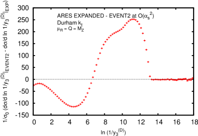
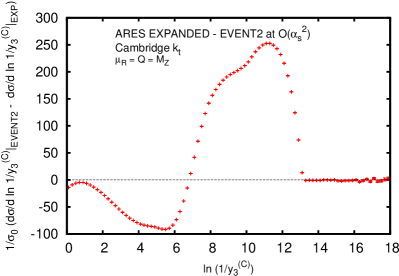
Figure 1: Difference of the three-jet resolution differential distributions between Event2 and the ${\cal O}(\alpha_{s}^{2})$ expansion of the resummation performed in this letter.

Since the two observables in this case are identical for a single emission, it is useful to perform a similar check on the difference

$$\frac{1}{\sigma_{0}}\left(\frac{d\sigma}{d\ln(1/y_{3}^{(D)})}-\frac{d\sigma}{d\ln(1/y_{3}^{(C)})}\right)\,.$$ (55)

Taking the difference in eq. (55) leads to numerically more stable fixed-order results. The corresponding check is shown in fig. 2.

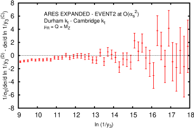
Figure 2: Difference of the three-jet resolution differential distribution between the Durham and the Cambridge algorithm as computed in Event2 minus the ${\cal O}(\alpha_{s}^{2})$ expansion of the resummation performed in this letter.

References

• (1) G.Β Altarelli, Ann.Β Rev.Β Nucl.Β Part.Β Sci.Β  39 (1989) 357.
• (2) S.Β Bethke and J.Β E.Β Pilcher, Ann.Β Rev.Β Nucl.Β Part.Β Sci.Β  42 (1992) 251.
• (3) A.Β Gehrmann-De Ridder, T.Β Gehrmann, E.Β W.Β N.Β Glover and G.Β Heinrich, JHEP 0712 (2007) 094 [arXiv:0711.4711 [hep-ph]].
• (4) A.Β Gehrmann-De Ridder, T.Β Gehrmann, E.Β W.Β N.Β Glover and G.Β Heinrich, Phys.Β Rev.Β Lett.Β  100 (2008) 172001 [arXiv:0802.0813 [hep-ph]].
• (5) S.Β Weinzierl, Phys.Β Rev.Β Lett.Β  101 (2008) 162001 [arXiv:0807.3241 [hep-ph]].
• (6) S.Β Weinzierl, JHEP 0906 (2009) 041 [arXiv:0904.1077 [hep-ph]].
• (7) V.Β Del Duca, C.Β Duhr, A.Β Kardos, G.Β Somogyi, Z.Β Szor, Z.Β Trocsanyi and Z.Β Tulipant, arXiv:1606.03453 [hep-ph].
• (8) S.Β Catani, Y.Β L.Β Dokshitzer, M.Β Olsson, G.Β Turnock and B.Β R.Β Webber, Phys.Β Lett.Β B 269 (1991) 432.
• (9) D.Β de Florian and M.Β Grazzini, Nucl.Β Phys.Β B 704 (2005) 387 [hep-ph/0407241].
• (10) T.Β Becher and M.Β D.Β Schwartz, JHEP 0807 (2008) 034 [arXiv:0803.0342 [hep-ph]].
• (11) Y.Β T.Β Chien and M.Β D.Β Schwartz, JHEP 1008 (2010) 058 [arXiv:1005.1644 [hep-ph]].
• (12) T.Β Becher and G.Β Bell, JHEP 1211 (2012) 126 [arXiv:1210.0580 [hep-ph]].
• (13) A.Β H.Β Hoang, D.Β W.Β Kolodrubetz, V.Β Mateu and I.Β W.Β Stewart, Phys.Β Rev.Β D 91 (2015) no.9, 094017 [arXiv:1411.6633 [hep-ph]].
• (14) A.Β Banfi, H.Β McAslan, P.Β F.Β Monni and G.Β Zanderighi, JHEP 1505 (2015) 102 [arXiv:1412.2126 [hep-ph]].
• (15) T.Β Becher, X.Β Garcia i Tormo and J.Β Piclum, Phys.Β Rev.Β D 93 (2016) no.5, 054038 Erratum: [Phys.Β Rev.Β D 93 (2016) no.7, 079905] [arXiv:1512.00022 [hep-ph]].
• (16) C.Β Frye, A.Β J.Β Larkoski, M.Β D.Β Schwartz and K.Β Yan, arXiv:1603.06375 [hep-ph].
• (17) C.Β Frye, A.Β J.Β Larkoski, M.Β D.Β Schwartz and K.Β Yan, arXiv:1603.09338 [hep-ph].
• (18) A.Β Banfi, G.Β P.Β Salam and G.Β Zanderighi, JHEP 0201 (2002) 018 [hep-ph/0112156].
• (19) R.Β Abbate, M.Β Fickinger, A.Β H.Β Hoang, V.Β Mateu and I.Β W.Β Stewart, Phys.Β Rev.Β D 83 (2011) 074021 [arXiv:1006.3080 [hep-ph]].
• (20) A.Β H.Β Hoang, D.Β W.Β Kolodrubetz, V.Β Mateu and I.Β W.Β Stewart, Phys.Β Rev.Β D 91 (2015) no.9, 094018 [arXiv:1501.04111 [hep-ph]].
• (21) T.Β Gehrmann, G.Β Luisoni and P.Β F.Β Monni, Eur.Β Phys.Β J.Β C 73 (2013) no.1, 2265 [arXiv:1210.6945 [hep-ph]].
• (22) S.Β Bethke, G.Β Dissertori and G.Β P.Β Salam, EPJ Web Conf.Β  120 (2016) 07005.
• (23) G.Β Dissertori, A.Β Gehrmann-De Ridder, T.Β Gehrmann, E.Β W.Β N.Β Glover, G.Β Heinrich and H.Β Stenzel, Phys.Β Rev.Β Lett.Β  104 (2010) 072002 [arXiv:0910.4283 [hep-ph]].
• (24) S.Β Bethke et al. [JADE Collaboration], Eur.Β Phys.Β J.Β C 64 (2009) 351 [arXiv:0810.1389 [hep-ex]].
• (25) G.Β Dissertori, A.Β Gehrmann-De Ridder, T.Β Gehrmann, E.Β W.Β N.Β Glover, G.Β Heinrich, G.Β Luisoni and H.Β Stenzel, JHEP 0908 (2009) 036 [arXiv:0906.3436 [hep-ph]].
• (26) G.Β Abbiendi et al. [OPAL Collaboration], Eur.Β Phys.Β J.Β C 71 (2011) 1733 [arXiv:1101.1470 [hep-ex]].
• (27) A.Β Heister et al. [ALEPH Collaboration], Eur.Β Phys.Β J.Β C 35 (2004) 457.
• (28) J.Β Abdallah et al. [DELPHI Collaboration], Eur.Β Phys.Β J.Β C 29 (2003) 285 [hep-ex/0307048].
• (29) B.Β Adeva et al. [L3 Collaboration], Z.Β Phys.Β C 55 (1992) 39.
• (30) P.Β Achard et al. [L3 Collaboration], Phys.Β Rept.Β  399 (2004) 71 [hep-ex/0406049].
• (31) G.Β Abbiendi et al. [OPAL Collaboration], Eur.Β Phys.Β J.Β C 40 (2005) 287 [hep-ex/0503051].
• (32) Y.Β L.Β Dokshitzer, G.Β D.Β Leder, S.Β Moretti and B.Β R.Β Webber, JHEP 9708 (1997) 001 [hep-ph/9707323].
• (33) S.Β Bentvelsen and I.Β Meyer, Eur.Β Phys.Β J.Β C 4 (1998) 623 [hep-ph/9803322].
• (34) A.Β Banfi, G.Β P.Β Salam and G.Β Zanderighi, JHEP 0503 (2005) 073 [hep-ph/0407286].
• (35) A.Β Banfi, H.Β McAslan, P.Β F.Β Monni and G.Β Zanderighi, supplemental material, available at the end of the arXiv version of this article.
• (36) A.Β Banfi, P.Β F.Β Monni, G.Β P.Β Salam and G.Β Zanderighi, Phys.Β Rev.Β Lett.Β  109 (2012) 202001 [arXiv:1206.4998 [hep-ph]].
• (37) S.Β Weinzierl, Eur.Β Phys.Β J.Β C 71 (2011) 1565 Erratum: [Eur.Β Phys.Β J.Β C 71 (2011) 1717] [arXiv:1011.6247 [hep-ph]].
• (38) M.Β Cacciari, G.Β P.Β Salam and G.Β Soyez, Eur.Β Phys.Β J.Β C 72 (2012) 1896 doi:10.1140/epjc/s10052-012-1896-2 [arXiv:1111.6097 [hep-ph]].
• (39) A.Β Banfi, G.Β P.Β Salam and G.Β Zanderighi, Eur.Β Phys.Β J.Β C 47 (2006) 113 [hep-ph/0601139].
• (40) A.Β Gehrmann-De Ridder, T.Β Gehrmann, E.Β W.Β N.Β Glover and G.Β Heinrich, Comput.Β Phys.Β Commun.Β  185 (2014) 3331 [arXiv:1402.4140 [hep-ph]].
• (41) S.Β Catani and M.Β H.Β Seymour, Nucl.Β Phys.Β B 485 (1997) 291 [Erratum-ibid.Β B 510 (1998) 503] [hep-ph/9605323].