Proximal Quasi-Newton Methods for Regularized Convex Optimization with Linear and Accelerated Sublinear Convergence Rates

Abstract

A general, inexact, efficient proximal quasi-Newton algorithm for composite optimization problems has been proposed by Scheinberg and Tang [Math. Program., 160 (2016), pp. 495-529] and a sublinear global convergence rate has been established. In this paper, we analyze the global convergence rate of this method, both in the exact and inexact setting, in the case when the objective function is strongly convex. We also investigate a practical variant of this method by establishing a simple stopping criterion for the subproblem optimization. Furthermore, we consider an accelerated variant, based on FISTA of Beck and Teboulle [SIAM J. Optim., 2 (2009), pp. 183-202], to the proximal quasi-Newton algorithm. Jiang, Sun, and Toh [SIAM J. Optim., 22 (2012), pp. 1042-1064] considered a similar accelerated method, where the convergence rate analysis relies on very strong impractical assumptions on Hessian estimates. We present a modified analysis while relaxing these assumptions and perform a numerical comparison of the accelerated proximal quasi-Newton algorithm and the regular one. Our analysis and computational results show that acceleration may not bring any benefit in the quasi-Newton setting.

1 Introduction

We address the convex optimization problem of the form

$$\min_{x}\{F(x):=f(x)+g(x),~{}x\in\mathbb{R}^{n}\},$$ (1)

where $g:\mathbb{R}^{n}\rightarrow\mathbb{R}$ is a continuous convex function which is possibly nonsmooth and $f:\mathbb{R}^{n}\rightarrow\mathbb{R}$ is a convex continuously differentiable function with Lipschitz continuous gradient, i.e.

$$\|\nabla f(x)-\nabla f(y)\|_{2}\leq L\|x-y\|_{2}~{}~{}~{}\text{for every}~{}~{}x,y\in\mathbb{R}^{n},$$

where $L$ is the global Lipschitz constant of the gradient $\nabla f$. This class of problems, when $g(x)=\lambda\|x\|_{1}$, contains some of the most common machine learning models such as sparse logistic regression lin ; shalev , sparse inverse covariance selection hsieh ; olsen ; rish , and unconstrained Lasso tibshirani .

The Proximal Gradient Algorithm (PGA) is a variant of the proximal methods and is a well-known first-order method for solving optimization problem (1). Although classical subgradient methods can be applied to problem (1) when $g$ is nonsmooth, they can only achieve the rate of convergence of $\mathcal{O}(1/\sqrt{k})$ nesterov2 , while PGA converges at a rate of $\mathcal{O}(1/k)$ in both smooth and nonsmooth cases nesterov4 ; beck . In order to improve the global sublinear rate of convergence of PGA further, the Accelerated Proximal Gradient Algorithm (APGA) has been originally proposed by Nesterov in nesterov3 , and refined by Beck and Teboulle in beck . It has been shown that the APGA provides a significant improvement compared to PGA, both theoretically, with a rate of convergence of $\mathcal{O}({1}/{k^{2}})$, and practically beck . This rate of convergence is known to be the best that can be obtained using only first-order information yudin ; nesterov2 ; goldfarb , causing APGA to be known as an optimal first-order method. The class of accelerated methods contains many variants that share the same convergence rates and use only first-order information nesterov2 ; nesterov5 ; tseng . The main known drawback of most of the variants of APGA is that the sequence of the step-size $\{\mu_{k}\}$ has to be nonincreasing. This theoretical restriction sometimes has a big impact on the performance of this algorithm in practice. In goldfarb , in order to overcome this difficulty, a new version of APGA has been proposed. This variant of APGA allows to increase step-sizes from one iteration to the next, but maintain the same rate of convergence of $\mathcal{O}({1}/{k^{2}})$. In particular, the authors have shown that a full backtracking strategy can be applied in APGA and that the resulting complexity of the algorithm depends on the average value of step-size parameters, which is closely related to local Lipschitz constants, rather than the global one.

To make PGA and APGA practical, for some complicated instances of (1), one needs to allow for inexact computations in the algorithmic steps. In mark , inexact variants of PGA and APGA have been analyzed with two possible sources of error: one in the calculation of the gradient of the smooth term and the other in the proximal operator with respect to the nonsmooth part. The convergence rates are preserved if the sequence of errors converges to zero sufficiently fast. Moreover, it has been shown that both of these algorithms obtain a linear rate of convergence, when the smooth term $f$ is strongly convex. Recently, in dmitri , the linear convergence of PGA has been shown under the quadratic growth condition, which is weaker than a strong convexity assumption. In particular, their analysis relies on the fact that PGA linearly bounds the distance to the solution set by the step lengths. This property, called an error bound condition, has been proved to be equivalent to the standard quadratic growth condition. More precisely, a strong convexity assumption is a sufficient, but not a necessary condition for this error bound property.

While PGA and APGA can be efficient in solving (1), it has been observed that using (partial) second-order information often significantly improves the performance of the algorithms. Hence, Newton type proximal algorithms, also known as the proximal Newton methods, have become popular sra ; olsen ; lee ; nocedal3 ; tang and are often the methods of choice. When accurate (or nearly accurate) second-order information is used, the method no longer falls in the first-order category and faster convergence rates are expected, at least locally. Indeed, the global convergence and the local superlinear rate of convergence of the Proximal Quasi-Newton Algorithm (PQNA) are presented in lee and nocedal3 , respectively for both the exact and inexact settings. However, in the case of limited memory BFGS method nocedal1 ; nocedal2 , the method is still essentially a first-order method. While practical performance may be by far superior, the rates of convergence are at best the same as those of the pure first-order counterparts. In tang , an inexact PQNA with global sublinear rate of $\mathcal{O}({1}/{k})$ is proposed. While the algorithm can use any positive definite Hessian estimates, as long as their eigenvalues are uniformly bounded above and away from zero, the practical implementation proposed in tang used a limited memory BFGS Hessian approximation. The inexact setting of the algorithm allows for a relaxed sufficient decrease condition as well as an inexact subproblem optimization, for example via coordinate descent.

In this work, we show that PQNA, as proposed in tang , using general Hessian estimates $H_{k}$, has the linear convergence rate in the case of strongly convex smooth term $f$. Moreover, we consider an inexact variant, similar to the ones in nocedal3 ; tang , allowing inexact subproblem solutions as well as a relaxed sufficient decrease condition. In order to control the errors in the inexact subproblem optimization, we establish a simple stopping criterion for the subproblem solver, based on the iteration count, which guarantees that the inner subproblem is solved to the required accuracy. In contrast, in related works toh ; villa , it is assumed that an approximate subproblem solver yields an approximate subdifferential, which is a strong assumption on the subproblem solver which also does not clearly result in a simple stopping criterion.

Next, we apply Nesterov’s acceleration scheme to PQNA as proposed in tang , with a view of developing a version of this algorithm with faster convergence rates in the general convex case. In toh , the authors have introduced the Accelerated Proximal Quasi-Newton Algorithm (APQNA) with rate of convergence of $\mathcal{O}({1}/{k^{2}})$. However, this rate of convergence is achieved under condition $0\prec H_{k}\preceq H_{k-1}$, on the Hessian estimate $H_{k}$, at each iteration $k$. At the same time, this sequence of matrices has to be chosen so that $H_{k}$ is sufficiently positive definite to provide an overapproximation of $f$. Hence, these two conditions may contradict with each other unless the sequence of $\{H_{k}\}$ consists of unnecessarily large matrices. Moreover, in a particular case, when $H_{k}$ is set to be a scalar multiple of the identity, i.e., $H_{k}=\frac{1}{\mu_{k}}I$, then assumption $0\prec H_{k}\preceq H_{k-1}$ enforces $\mu_{k}\geq\mu_{k-1}$, implying nondecreasing step-size parameters, which contradicts the standard condition of APGA, which is $\mu_{k}\leq\mu_{k-1}$.

In this work, we introduce a new variant of APQNA, where we relax the restrictive assumptions imposed in toh . We use the scheme, originally introduced in goldfarb , which allows for the increasing and decreasing step-size parameters. We show that our version of APQNA achieves the convergence rate of $\mathcal{O}(1/k^{2})$ under some assumptions on the Hessian estimates. While we show that this assumption is rather strong and may not be satisfied by general matrices, it is not contradictory. Firstly, our result applies under the same restrictive condition from toh . We also show that our condition on the matrices holds in the case when the approximate Hessian at each iteration is a scaled version of the same “fixed” matrix $H$, which is a generalization of APGA. We investigate the performance of this algorithm in practice, and discover that this restricted version of a proximal quasi-Newton method is quite effective in practice. We also demonstrate that the general L-BFGS based PQNA does not benefit from the acceleration, which supports our analysis of the theoretical limitations.

This paper is organized as follows. In the next section, we describe the basic definitions and existing algorithms, PGA, APGA and PQNA, that we refer to later in the paper. In Section 3, we analyze PQNA in the strongly convex case. In Section 4, we propose, state and analyze a general APQNA and its simplified version. We present computational results in Section 5. Finally, we state our conclusions in Section 6.

2 Notation and Preliminaries

In this work, the Euclidean norm $\|a\|^{2}:=a^{T}a$, and the inner product $\langle a,b\rangle:=a^{T}b$, are also defined in the scaled setting such that, $\|a\|^{2}_{H}:=a^{T}Ha$, and $\langle a,b\rangle_{H}:=a^{T}Hb$. We denote the identity matrix by $I\in\mathbb{R}^{n\times n}$. The vector $e_{j}$ stands for a unit vector along the $j$-th coordinate. We use $x_{k}$ to denote the approximate minimizer (the iterate), computed at iteration $k$ of an appropriate algorithm, and $x_{*}$ to denote an exact minimizer of $F$. Finally, $(\partial F(x))_{\text{min}}$ denotes the minimum norm subgradient of function $F$ at point $x$.

The proximal mapping of a convex function $g$ at a given point $v$, with parameter $\mu$ is defined as

$$prox_{g}^{\mu}(v):=\arg\min_{u\in\mathbb{R}^{n}}\{g(u)+\frac{1}{2\mu}\|u-v\|^{2}\},~{}~{}~{}\text{where}~{}~{}\mu>0.$$ (2)

The proximal mapping is the base operation of the proximal methods. In order to solve the composite problem (1), each iteration of PGA computes the proximal mapping of the function $g$ at point $x_{k}-\mu_{k}\nabla f(x_{k})$ as follows:

$$p_{\mu_{k}}(x_{k}) :=prox_{g}^{\mu_{k}}(x_{k}-\mu_{k}\nabla f(x_{k}))$$ (3)

$$:=\arg\min_{u\in\mathbb{R}^{n}}\{g(u)+f(x_{k})+\langle\nabla f(x_{k}),u-x_{k}\rangle+\frac{1}{2\mu_{k}}\|u-x_{k}\|^{2}\}.$$

We will call the objective function, that is minimized in (3), a composite quadratic approximation of the convex function $F(x):=f(x)+g(x)$. This approximation at a given point $v$, for a given $\mu$ is defined as

$$Q_{\mu}(u,v):=f(v)+\nabla f(v)^{T}(u-v)+\frac{1}{2\mu}\|u-v\|^{2}+g(u).$$ (4)

Then, the proximal operator can be written as

$$p_{\mu}(v):=\arg\min_{u\in\mathbb{R}^{n}}Q_{\mu}(u,v).$$

Using this notation we first present the basic PGA framework with backtracking over $\mu$ in Algorithm 1. The simple backtracking scheme enforces that the sufficient decrease condition

$$F(x_{k+1})\leq Q_{\mu_{k}}(x_{k+1},x_{k})\leq Q_{\mu_{k}}(x_{k},x_{k})=F(x_{k}),$$ (5)

holds. This condition is essential in the convergence rate analysis of PGA and is easily satisfied when $\mu\leq{1}/{L}$. The backtracking is used for two reasons–because the constant $L$ may not be known and because $\mu\leq{1}/{L}$ may be too pessimistic, i.e., condition (5) may be satisfied for much larger values of $\mu$ allowing for larger steps.

Algorithm 1 Proximal Gradient Algorithm

1: 

2:Initialize $x_{0}\in\mathbb{R}^{n}$, and choose $\beta\in(0,1)$.

3:for $k=1,2,\cdots$ do

4:    Choose $\mu_{k}^{0}$ and define $\mu_{k}:=\mu_{k}^{0}$.

5:    Compute $p_{\mu_{k}}(x_{k}):=\arg\min_{u\in\mathbb{R}^{n}}Q_{\mu_{k}}(u,x_{k})$.

6:    while $F\left(p_{\mu_{k}}(x_{k})\right)>Q_{\mu_{k}}\left(p_{\mu_{k}}(x_{k}),x_{k}\right)$ do

7:         Set $\mu_{k}\leftarrow\beta\mu_{k}$.

8:         Compute $p_{\mu_{k}}(x_{k}):=\arg\min_{u\in\mathbb{R}^{n}}Q_{\mu_{k}}(u,x_{k})$.     

9:    Set $x_{k+1}\leftarrow p_{\mu_{k}}(x_{k})$.

We now present the accelerated variant of PGA stated as APGA, where at each iteration $k$, instead of constructing $Q_{\mu_{k}}$ at the current minimizer $x_{k}$, it is constructed at a different point $y_{k}$, which is chosen as a specific linear combination of the latest two or more minimizers, e.g.

$$y_{k+1}=x_{k}+\alpha_{k}(x_{k}-x_{k-1}),$$

where the sequence $\{\alpha_{k}\}$ is chosen in such a way to guarantee an accelerated convergence rate as compared to the original PGA. Algorithm 2 is a variant of APGA framework, often referred to as FISTA, presented in beck , where $\alpha_{k}=({t_{k}-1})/({t_{k+1}})$. In this work, we choose to focus on FISTA algorithm specifically. The choice of the accelerated parameter $t_{k+1}$ in (6a) is dictated by the analysis of the complexity of FISTA beck and the condition $\mu_{k+1}\leq\mu_{k}$ that is imposed by the initialization of the backtracking procedure with $\mu_{k+1}^{0}:=\mu_{k}$. In goldfarb , the definition of $t_{k+1}$ was generalized to allow $\mu_{k+1}^{0}>\mu_{k}$, while retaining the convergence rate. We will use a similar technique in our proposed APQNA.

Algorithm 2 Accelerated Proximal Gradient Algorithm

1: 

2:Initialize $t_{1}=1$, $\mu_{1}^{0}>0$, and $y_{1}=x_{0}\in\mathbb{R}^{n}$, and choose $\beta\in(0,1)$.

3:for $k=1,2,\cdots$ do

4:    Define $\mu_{k}:=\mu_{k}^{0}$.

5:    Compute $p_{\mu_{k}}(y_{k}):=\arg\min_{u\in\mathbb{R}^{n}}Q_{\mu_{k}}(u,y_{k})$.

6:    while $F\left(p_{\mu_{k}}(y_{k})\right)>Q_{\mu_{k}}\left(p_{\mu_{k}}(y_{k}),y_{k}\right)$ do

7:         Set $\mu_{k}\leftarrow\beta\mu_{k}$.

8:         Compute $p_{\mu_{k}}(y_{k}):=\arg\min_{u\in\mathbb{R}^{n}}Q_{\mu_{k}}(u,y_{k})$.     

9:    Set $x_{k}\leftarrow p_{\mu_{k}}(y_{k})$.

10:    Define $\mu_{k+1}^{0}:=\mu_{k}$ and compute $t_{k+1}$ and $y_{k+1}$, so that

$$t_{k+1}=\frac{1}{2}\left(1+\sqrt{1+4t_{k}^{2}}\right)$$ (6a)

and $$y_{k+1}=x_{k}+\frac{t_{k}-1}{t_{k+1}}\left(x_{k}-x_{k-1}\right).$$ (6b)

In this work, we are interested in the extensions of the above proximal methods, which utilize an approximation function $Q_{\mu}$, using partial second-order information about $f$. These quasi-Newton type proximal algorithms use a generalized form of the proximal operator (2), known as the scaled proximal mapping of $g$, which are defined for a given point $v$ as

$$prox_{g}^{H}(v):=\arg\min_{u\in\mathbb{R}^{n}}\{g(u)+\frac{1}{2}\|u-v\|_{H}^{2}\},$$

where matrix $H$ is a positive definite matrix. In particular, the following operator

$$p_{H_{k}}(x_{k}) :=prox_{g}^{H_{k}}\left(x_{k}-H_{k}^{-1}\nabla f(x_{k})\right),$$ (7)

computes the minimizer, over $u$, of the following composite quadratic approximation of function $F$

$$Q_{H}(u,v):=f(v)+\langle\nabla f(v),u-v\rangle+\frac{1}{2}\|u-v\|_{H}^{2}+g(u),$$ (8)

when $v=x_{k}$. Matrix $H$ is the approximate Hessian of $f$ and its choice plays the key role in the quality of this approximation. Clearly, when $H=\frac{1}{\mu}I$, approximation (8) converts to (4), which is used throughout PGA. If we set $H=\nabla^{2}f(v)$, then (8) is the second-order Taylor approximation of $F$. At each iteration of PQNA the following optimization problem needs to be solved

$$p_{H}(v):=\arg\min_{u\in\mathbb{R}^{n}}Q_{H}(u,v),$$ (9)

which we assume to be computationally inexpensive relative to solving (1) for any $v\in\mathbb{R}^{n}$ and some chosen class of positive definite approximate Hessian $H$. Our assumption is motivated by tang , where it is shown that for L-BFGS Hessian approximation, problem (9) can be solved efficiently and inexactly via coordinate descent method. Specifically, the proximal operator (7) does not have closed form solution for most types of Hessian estimates $H_{k}$ and most nonsmooth terms $g$, such as $g=\lambda\|x\|_{1}$, when (7) is a convex quadratic optimization problem. Hence, it may be too expensive to seek the exact solution of subproblem (7) on every iteration. In tang , an efficient version of PQNA is proposed that constructs Hessian estimates based on the L-BFGS updates, resulting in $H_{k}$ matrices that are sum of a diagonal and a low rank matrix. The resulting subproblem, structured as (7), is then solved up to some expected accuracy via randomized coordinate descent, which effectively exploits the special structure of $H_{k}$. The analysis in tang shows that the resulting inexact PQNA converges sublinearly if the Hessian estimates remain positive definite and bounded, without assuming any other structure. In this paper, all the theory is derived for arbitrary positive definite Hessian estimates, without any assumption on their structure, or how closely they are representing the true Hessian. In our implementation, however, we will construct the Hessian estimates via L-BFGS as it is done in tang . The framework of the inexact variant of PQNA for general approximate Hessian is stated in Algorithm 3. In this algorithm, the inexact solution of (9) is denoted by $p_{H,\epsilon}(v)$, as an $\epsilon-$minimizer of the subproblem that satisfies

$$g(p_{H,\epsilon}(v))+\frac{1}{2}\|p_{H,\epsilon}(v)-z\|_{H}^{2}\leq\min_{u\in\mathbb{R}^{n}}\{g(u)+\frac{1}{2}\|u-z\|_{H}^{2}\}+\epsilon,$$ (10)

where $z:=v-H^{-1}\nabla f(v)$. Obtaining such an inexact solution can be achieved by applying any linearly convergent algorithm, as will be discussing in detail at the end of this section.

In addition, for a given $\eta\in(0,1]$, the typical condition (5), used in beck and bach , is relaxed by using a trust-region like sufficient decrease condition

$$\left(F\left(p_{H,\epsilon}(v)\right)-F(v)\right)\leq\eta\left(Q_{H}\left(p_{H,\epsilon}(v),v\right)-F(v)\right).$$ (11)

This relaxed condition was proposed and tested in tang for PQNA and was shown to lead to superior numerical performance, saving multiple backtracking steps during the earlier iterations of the algorithm. Note that, one can obtain the exact version of Algorithm 3 by replacing $p_{H_{k},\epsilon_{k}}$ with $p_{H_{k}}$, and setting $\eta=1$.

Algorithm 3 Inexact Proximal Quasi-Newton Algorithm

1: 

2:Initialize $x_{0}\in\mathbb{R}^{n}$, and choose $\beta\in(0,1)$ and $\eta\in(0,1]$.

3:for $k=1,2,\cdots$ do

4:    Choose $\mu_{k}>0$ and bounded $G_{k}\succeq 0$.

5:    Define $H_{k}:=G_{k}+\frac{1}{2\mu_{k}}I$.

6:    Compute $p_{H_{k},\epsilon_{k}}(x_{k})$ such that (10) is satisfied.

7:    while $\left(F\left(p_{H_{k},\epsilon_{k}}(x_{k})\right)-F(x_{k})\right)>\eta\left(Q_{H_{k}}\left(p_{H_{k},\epsilon_{k}}(x_{k}),x_{k}\right)-F(x_{k})\right)$ do

8:         Set $\mu_{k}\leftarrow{\beta}\mu_{k}$.

9:         Update $H_{k}$ via $H_{k}:=G_{k}+\frac{1}{2\mu_{k}}I$.

10:         Compute $p_{H_{k},\epsilon_{k}}(x_{k})$ such that (10) is satisfied.     

11:    Set $x_{k+1}\leftarrow p_{H_{k},\epsilon_{k}}(x_{k})$.

Throughout our analysis, we make the following assumptions.

Assumption 2.1

• $f$ is convex with Lipschitz continuous gradient with constant $L$.

• $g$ is a lower semi-continuous proper convex function.

• There exists an $x_{*}\in\mathbb{R}^{n}$, which is a minimizer of $F$.

• There exists positive constants $m$ and $M$ such that, for all $k>0$,

  $$mI\preceq H_{k}\preceq MI.$$ (12)

Remark 1

In Algorithm 3, as long as the sequence of positive definite matrices $G_{k}$ has uniformly bounded eigenvalues, condition (12) is satisfied. In fact, since the sufficient decrease condition in Step 3 is satisfied for $H_{k}\succeq LI$, then it is satisfied when $\mu_{k}\leq{1}/{L}$. Hence, at each iteration we have a finite and bounded number of backtracking steps and the resulting $H_{k}$ has bounded eigenvalues. The lower bound on the eigenvalues of $H_{k}$ is simply imposed either by choosing a positive definite $G_{k}$ or bounding $\mu_{k}^{0}$ from above.

In the next section, we analyze the convergence properties of PQNA when $f$ in (1) is strongly convex.

3 Analysis of the Proximal Quasi-Newton Algorithm under Strong Convexity

In this section, we analyze the convergence properties of PQNA to solve problem (1), in the case when the smooth function $f$ is $\gamma-$strongly convex. In particular, the following assumption is made throughout this section.

Assumption 3.1

For all $x$ and $y$ in $\mathbb{R}^{n}$, and any $t\in[0,1]$, the following two equivalent conditions hold.

$$\gamma\|x-y\|^{2}\leq\langle\nabla f(x)-\nabla f(y),x-y\rangle$$ (13a)

and $$f\left(tx+(1-t)y\right)\leq tf(x)+(1-t)f(y)-\frac{1}{2}\gamma t(1-t)\|x-y\|^{2}.$$ (13b)

To establish a linear convergence rate of PQNA, we consider extending two different approaches used to show a similar result for PGA. The first approach we consider can be found in phd , and is based on the proof techniques used in dmitri for PGA. The reason we chose the approach in dmitri is due to the fact that the linear rate of convergence is shown under the quadratic growth condition, which is a relaxation of the strong convexity. Hence, extending this analysis to PQNA, as a subject of a future work, may allow us to relax the strong convexity assumption for this algorithm as well. However, there appears to be some limitations in the extension of this analysis phd , in particular in the inexact case. This observation motivates us to present the approach used in nesterov4 to analyze convergence properties of inexact PQNA. As we see below, this analysis readily extends to our case and allows us to establish simple rules for subproblem solver termination to achieve the desired subproblem accuracy.

3.1 Convergence Analysis

Let us consider Algorithm 3 for which (10) holds for some sequence of errors $\epsilon_{k}\geq 0$. The relaxed sufficient decrease condition

$$F(x_{k+1})-F(x_{k})\leq\eta(Q_{H_{k}}(x_{k+1},x_{k})-F(x_{k})),$$

for a given $\eta\in(0,1]$, can be written as

$$F(x_{k+1}) \leq Q_{H_{k}}(x_{k+1},x_{k})-(1-\eta)\left(Q_{H_{k}}(x_{k+1},x_{k})-F(x_{k})\right)$$

$$\leq Q_{H_{k}}(x_{k+1},x_{k})-\frac{1-\eta}{\eta}\left(F(x_{k+1})-F(x_{k})\right).$$

Thus, at each iteration we have

$$F(x_{k+1})\leq Q_{H_{k}}(x_{k+1},x_{k})+\xi_{k},$$ (14)

where the sequence of the errors $\xi_{k}$ is defined as

$$\xi_{k}\leq(1-\frac{1}{\eta})\left(F(x_{k+1})-F(x_{k})\right).$$ (15)

In particular, setting $\eta=1$ results in $\xi_{k}=0$, for all $k$ and enforces the algorithm to accept only those steps that achieve full (predicted) reduction. However, using $\eta<1$ allows the algorithm to take steps satisfying only a fraction of the predicted reduction, which may lead to larger steps and faster progress.

Under the above inexact condition, we can show the following result.

Theorem 3.2

Suppose that Assumptions 2.1 and 3.1 hold. At each iteration of the inexact PQNA, stated in Algorithm 3, we have

$$F(x_{k})-F(x_{*})\leq\rho^{k}\left(F(x_{0})-F(x_{*})+A_{k}\right),$$ (16)

when $\rho=1-{(\eta\gamma)}/{(\gamma+M)}$, and

$$A_{k}:=\eta\sum_{i=1}^{k}\left({\epsilon_{i}}/{\rho^{i}}\right).$$

Proof

Applying (14), with $v=x_{k}$ and consequently $p_{H_{k},\epsilon_{k}}(x_{k})=x_{k+1}$, we have

$$F(x_{k+1}) \leq Q_{H_{k}}(x_{k+1},x_{k})+\xi_{k}$$

$$=f(x_{k})+\langle\nabla f(x_{k}),x_{k+1}-x_{k}\rangle+\frac{1}{2}\|x_{k+1}-x_{k}\|_{H_{k}}^{2}+g(x_{k+1})+\xi_{k}$$

$$=\min_{u\in\mathbb{R}^{n}}~{}f(x_{k})+\langle\nabla f(x_{k}),u-x_{k}\rangle+\frac{1}{2}\|u-x_{k}\|_{H_{k}}^{2}+g(u)+\epsilon_{k}+\xi_{k}$$

$$\leq\min_{u\in\mathbb{R}^{n}}~{}f(u)+\frac{1}{2}\|u-x_{k}\|_{H_{k}}^{2}+g(u)+(\epsilon_{k}+\xi_{k})~{}~{}~{}~{}~{}\left(\text{convexity of $f$}\right)$$

$$=\min_{u\in\mathbb{R}^{n}}~{}F(u)+\frac{1}{2}\|x_{k}-u\|_{H_{k}}^{2}+(\epsilon_{k}+\xi_{k})$$

$$\leq\min_{t\in[0,1]}~{}F(tx_{*}+(1-t)x_{k})+\frac{1}{2}\|x_{k}-tx_{*}-(1-t)x_{k}\|_{H_{k}}^{2}$$

$$~{}+(\epsilon_{k}+\xi_{k})$$

$$\leq\min_{t\in[0,1]}~{}tF(x_{*})+(1-t)F(x_{k})-\frac{1}{2}\gamma t(1-t)\|x_{*}-x_{k}\|^{2}$$

$$~{}+\frac{1}{2}t^{2}\|x_{*}-x_{k}\|_{H_{k}}^{2}+(\epsilon_{k}+\xi_{k})~{}~{}~{}~{}(\text{using \eqref{def.strong}})$$

$$\leq\min_{t\in[0,1]}~{}tF(x_{*})+(1-t)F(x_{k})-\frac{1}{2}\gamma t(1-t)\|x_{*}-x_{k}\|^{2}$$

$$~{}+\frac{1}{2}Mt^{2}\|x_{*}-x_{k}\|^{2}+(\epsilon_{k}+\xi_{k})$$

$$\leq t^{\prime}F(x_{*})+(1-t^{\prime})F(x_{k})+(\epsilon_{k}+\xi_{k}).~{}~{}~{}~{}~{}~{}~{}~{}\left(\text{where $t^{\prime}=\frac{\gamma}{\gamma+M}$}\right)$$

Therefore, we have

$$F(x_{k+1})\leq t^{\prime}F(x_{*})+(1-t^{\prime})F(x_{k})+(\epsilon_{k}+\xi_{k}),$$

which implies

$$F(x_{k+1})-F(x_{*}) \leq(1-t^{\prime})(F(x_{k})-F(x_{*}))+(\epsilon_{k}+\xi_{k}).$$

Now, by substituting the expression for $\xi_{k}$, as stated in (15), we will have

$$F(x_{k+1})-F(x_{*})\leq\rho(F(x_{k})-F(x_{*}))+\eta\epsilon_{k},$$

where $\rho=1-\eta t^{\prime}$. Now, we can conclude the final result as

$$F(x_{k})-F(x_{*}) \leq\rho^{k}(F(x_{0})-F(x_{*}))+\sum_{i=1}^{k}\eta\rho^{k-i}\epsilon_{i}$$

$$=\rho^{k}\left(F(x_{0})-F(x_{*})+\eta\sum_{i=1}^{k}\left({\epsilon_{i}}/{\rho^{i}}\right)\right),$$

where $\rho=1-{(\eta\gamma)}/{(\gamma+M)}$. ∎

Remark 2

In Theorem 3.2, by setting $\epsilon_{k}=0$ and $\eta=1$, which implies $\xi_{k}=0$, we achieve the linear convergence rate of the exact variant of PQNA.

Remark 3

We have shown that the linear rate of PQNA is $\rho=1-{(\eta\gamma)}/{(\gamma+M)}$. As argued in Remark 1, $M$ is of the same order as $L$ in the worst case, hence in that case the linear rate of PQNA is the same as that of the simple PGA. However, it is easy to see that in the proof of Theorem 3.2, the linear rate is derived using the upper bound on $\|x_{*}-x_{k}\|_{H_{k}}^{2}$, where $H_{k}$ is the approximate Hessian on step $k$. Clearly, the idea of using the partial second-order information is to reduce the worst case bound of $H_{k}$ in general and consequently on $\|x_{*}-x_{k}\|_{H_{k}}^{2}$. In particular, obtaining a smaller bound $M_{k}$ on each iteration yields a larger convergence coefficient $\rho_{k}=1-{(\eta\gamma)}/{(\gamma+M_{k})}$. While for general $H_{k}$, we do not expect to improve upon the regular PGA in theory, this remark serves to explain the better performance of PQNA in practice.

Based on the result of Theorem 3.2, it follows that the boundedness of the sequence $\{A_{k}\}$ is a sufficient condition to achieve the linear convergence rate. Hence, the required condition on the sequence of errors is $\sum_{i=1}^{k}\left({\epsilon_{i}}/{\rho^{i}}\right)<\infty$. For all $i\leq k$, suppose that $\epsilon_{i}\leq C\rho^{i\cdot\delta}$, for some $\delta>1$ and some $C>0$. Then, we have $\sum_{i=1}^{k}\left({\epsilon_{i}}/{\rho^{i}}\right)\leq C\sum_{i=1}^{k}\rho^{i(\delta-1)}$, which is uniformly bounded for all $k$. Recall that the $k$-th subproblem $Q_{k}^{*}:=\min_{u\in\mathbb{R}^{n}}Q_{H_{k}}(u,x_{k})$ is a strongly convex function with strong convexity parameter at least $m$–the lower bound on the eigenvalues of $H_{k}$. Let us assume now that each subproblem is solved via an algorithm with a linear convergence rate for strongly convex problems. In particular, if the subproblem solver is applied for $r(k)$ iterations to the $k$-th subproblem, we have

$$\left(Q_{H_{k}}(u_{r(k)},x_{k})-Q_{k}^{*}\right)\leq\alpha\left(Q_{H_{k}}(u_{{r(k)}-1},x_{k})-Q_{k}^{*}\right),$$ (17)

where $\alpha\in(0,1)$. Our goal is to ensure that $\epsilon_{k}\leq C\rho^{k\cdot\delta}$, which can be achieved by applying sufficient number of iterations of the subproblem algorithm. To be specific, the following theorem characterizes this required bound on the number of inner iterations.

Theorem 3.3

Suppose that at the $k$-th iteration of Algorithm 3, after applying the subproblem solver satisfying (17) for $r(k)$ iterations, starting with $u_{0}=x_{k}$, we obtain solution $x_{k+1}=u_{r(k)}$. Let $r(k)$ satisfy

$${r(k)}\geq k\log_{1/\alpha}(1/\rho^{\delta}),$$ (18)

for some $\delta>1$, and $\rho$ defined in Theorem 3.2. Then

$$Q_{H_{k}}(x_{k+1},x_{k})-Q_{k}^{*}\leq C\rho^{k\cdot\delta},$$

holds for all $k$, with $C$ being the uniform bound on $Q_{H_{k}}(x_{k},x_{k})-Q_{k}^{*}$, and the linear convergence of Algorithm 3 is achieved.

Proof

First, assume that at the $k-$th iteration we have applied the subproblem solver for ${r(k)}$ iterations to minimize strongly convex function $Q_{H_{k}}$. Now, by combining $Q_{H_{k}}(u_{0},u_{0})-Q_{k}^{*}\leq C$ and (17), we can conclude the following upper bound, so that

$$Q_{H_{k}}(u_{r(k)},u_{0})-Q_{k}^{*}\leq\alpha^{r(k)}C.$$

Now, if $\alpha^{r(k)}C\leq\epsilon_{k}$, we can guarantee that $u_{r(k)}$ is an $\epsilon_{k}$-solution of the $k$-th subproblem, so that $Q_{H_{k}}(u_{r(k)},u_{0})\leq Q_{k}^{*}+\epsilon_{k}$. Now, assuming that $\rho$ is known, we can set the error rate of the $k$-th iteration as $\epsilon_{k}\leq C\rho^{k\cdot\delta}$, for a fixed $\delta>1$. In this case, the number of inner iterations which guarantees the $\epsilon_{k}$-minimizer will be

$${r(k)}\geq k\log_{1/\alpha}(1/\rho^{\delta}).$$

∎

Remark 4

Since subproblems are strongly convex, the required linear convergence rate for the subproblem solver, stated in (17), can be guaranteed via some basic first-order algorithms or their accelerated variants. However, one difficulty in obtaining lower bound (18) is that it depends on the prior knowledge of $\rho$ and $\alpha$. Consider the following simple modification of Theorem 3.3; instead of condition (18), consider $r(k)$ satisfying

$${r(k)}\geq k\log_{1/\alpha^{\prime}}({k}/{\ell}),$$ (19)

for any given $\ell>0$ and $\alpha^{\prime}\in(0,1)$. Then $\epsilon_{k}\leq C\left({\ell}/{k}\right)^{k}$ implies $\epsilon_{k}\leq C\rho^{k\cdot\delta}$, for sufficiently large $k$.

In the next subsection, we extend our analysis to the case of solving subproblems via the randomized coordinate descent, where at each iteration the desired error bound related to $\epsilon_{k}$ is only satisfied in expectation.

3.2 Solving Subproblems via Randomized Coordinate Descent

As we mentioned before, in order to achieve linear convergence rate of the inexact PQNA, any simple first-order method (such as PGA) can be applied. However, as discussed in tang , in the case when $g(x)=\lambda\|x\|_{1}$ and $H_{k}$ is sum of a diagonal and a low rank matrix, as in the case of L-BFGS approximations, the coordinate descent method is the most efficient approach to solve the strongly convex quadratic subproblems. In this case, each iteration of coordinate descent has complexity of $\mathcal{O}(m)$, where $m$ is the memory size of L-BFGS, which is usually chosen to be less than $20$, while each iteration of a proximal gradient method has complexity of $\mathcal{O}(nm)$ and each iteration of the Newton type proximal method has complexity of $\mathcal{O}(nm^{2})$. While more iterations of coordinate descent may be required to achieve the same accuracy, it tends to be the most efficient approach. To extend our theory of the previous section and to establish the bound on the number of coordinate descent steps needed to solve each subproblem, we utilize convergence results for the randomized coordinate descent martin , as is done in tang .

Algorithm 4 shows the framework of the randomized coordinate descent method, which can be used as a subproblem solver of Algorithm 3 and is identical to the method used in tang . In Algorithm 4, function $Q_{H}$ is iteratively minimized over a randomly chosen coordinate, while the other coordinates remain fixed.

Algorithm 4 Randomized Coordinate Descent Algorithm

1: 

2:Initialize point $v\in\mathbb{R}^{n}$ and required number of iterations $r>0$.

3:Set ${u_{0}}\leftarrow v$.

4:for $l=1,2,\cdots,r-1$ do

5:    Choose $j$ uniformly from $\{1,2,\cdots,n\}$.

6:    Compute $z^{*}:=\arg\min_{z\in\mathbb{R}^{n}}Q_{H}(u_{l}+ze_{j},v)$.

7:    Set $u_{l+1}\leftarrow u_{l}+z^{*}e_{j}$.

8:Return $u_{r}$.

In what follows, we restate Theorem 6 in martin , which establishes linear convergence rate of the randomized coordinate descent algorithm, in expectation, to solve strongly convex problems.

Theorem 3.4

Suppose we apply randomized coordinate descent for $r$ iterations, to minimize the $m$-strongly convex function $Q$ with $M$-Lipschitz gradient, to obtain the random point $u_{r}$.

When $u_{0}$ is the initial point and $Q^{*}:=\min_{u\in\mathbb{R}^{n}}Q_{H}(u,u_{0})$, for any $r$, we have

$$\mathbb{E}\left(Q_{H}(u_{r},u_{0})-Q^{*}\right)\leq\left(1-\frac{1-\phi_{m,M}}{n}\right)^{r}\left(Q_{H}(u_{0},u_{0})-Q^{*}\right),$$ (20)

where $\phi_{m}$ is defined as

$$\phi_{m,M}=\begin{cases}1-{m}/{4M}&\text{if}~{}~{}m\leq 2M,\\ {M}/{m}&\text{otherwise.}\end{cases}$$ (21)

Proof

The proof can be found in martin . ∎

Now, we want to analyze how we can utilize the result of Theorem 3.4 to achieve the linear convergence rate of inexact PQNA, in expectation. Toward this end, first we need the following theorem as the probabilistic extension of Theorem 3.2.

Theorem 3.5

Suppose that Assumptions 2.1 and 3.1 hold. At each iteration $k$ of the inexact PQNA, stated in Algorithm 3, assume that the error $\epsilon_{k}$ is a nonnegaitve random variable defined on some probability space with an arbitrary distribution. Then, we have

$$\mathbb{E}\left(F(x_{k})-F(x_{*})\right)\leq\rho^{k}\left(F(x_{0})-F(x_{*})+B_{k}\right),$$ (22)

when $\rho=1-{(\eta\gamma)}/{(\gamma+M)}$, and

$$B_{k}:=\eta\sum_{i=1}^{k}\left(\mathbb{E}({\epsilon_{i}})/{\rho^{i}}\right).$$

Proof

The proof is a trivial modification of that of Theorem 3.2. ∎

In what follows, we describe how the randomized coordinate descent method ensures the required accuracy of subproblems and consequently guarantees linear convergence of the inexact PQNA.

Theorem 3.6

Suppose that at the $k$-th iteration of Algorithm 3, after applying Algorithm 4 for $r(k)$ iterations, starting with $u_{0}=x_{k}$, we obtain solution $x_{k+1}=u_{r(k)}$. If

$${r(k)}\geq k\log_{1/\alpha_{n}}({k}/{\ell}),$$

where $\ell$ is any positive constant, $\alpha_{n}=\left(1-\frac{1-\phi_{m,M}}{n}\right)$ with $\phi_{m,M}$ defined in (21), and $C$ is the uniform bound on $Q_{H_{k}}(x_{k},x_{k})-Q_{k}^{*}$, then Algorithm 3, converges linearly with constant $\rho=1-{(\eta\gamma)}/{(\gamma+M)}$, in expectation.

Proof

Suppose that at the $k$-th iteration of Algorithm 3, we apply $r(k)$ steps of Algorithm 4 to minimize the strongly convex function $Q_{H_{k}}$. If $u_{r(k)}$ denotes the resulting random point, when $u_{0}$ is the initial point and $Q_{k}^{*}:=\min_{u\in\mathbb{R}^{n}}Q_{H_{k}}(u,u_{0})$, then based on Theorem 3.4 we have

$$\mathbb{E}\left(Q_{H_{k}}(u_{r(k)},u_{0})-Q_{k}^{*}\right)\leq\alpha_{n}^{r(k)}C,$$ (23)

where $\alpha_{n}=\left(1-\frac{1-\phi_{m,M}}{n}\right)$, with $\phi_{m,M}$ defined in (21), $Q_{H_{k}}(u_{0},u_{0})-Q_{k}^{*}$ is bounded from above by $C$. Now, based on the result of Theorem 3.5, if $\mathbb{E}(\epsilon_{k})\leq C(\ell/k)^{k}$ for some given positive constant $\ell$, then for sufficiently large $k$, we can guarantee that $B_{k}$ is uniformly bounded for all $k$, and consequently the linear convergence rate of Algorithm 3, in expectation is established. Now, by using (23), $E(\epsilon_{k})\leq C(\ell/k)^{k}$ simply follows from

$${r(k)}\geq k\log_{1/\alpha_{n}}({k}/{\ell}).$$

∎

Remark 5

The bound on the number of steps $r(k)\geq k\log_{1/\alpha_{n}}({k}/{\ell})$ for randomized coordinate descent differs from the bound $r(k)\geq k\log_{1/\alpha}({k}/{\ell})$ on the number of steps of a deterministic linear convergence method, such as PGA by the difference in constants $\alpha$ and $\alpha_{n}$. It can be easily shown that in the worst case $\alpha_{n}\approx\alpha/n$, and hence, the number of coordinate descent steps is around $n$ times larger than that of a proximal gradient method. On the other hand, each coordinate descent step is $n$ times less expensive and in many practical cases a modest number of iterations of randomized coordinate descent is sufficient. Discussions on this can be found in martin and tang as well as in Section 5.

4 Accelerated Proximal Quasi-Newton Algorithm

We now turn to an accelerated variant of PQNA. As we described in the introduction section, the algorithm proposed in toh is a proximal quasi-Newton variant of FISTA, described in Algorithm 2. In toh , the convergence rate of $\mathcal{O}({1}/{k^{2}})$ is shown under the condition that the Hessian estimates satisfy $0\prec H_{k}\preceq H_{k-1}$, at each iteration. On the other hand, the sequence $\{H_{k}\}$ is chosen so that the quadratic approximation of $f$ is an over approximation. This leads to an unrealistic setting where two possible contradictory conditions need to be satisfied and as mentioned earlier, this condition contradicts the assumptions of the original APGA, stated in Algorithm 2. We propose a more general version, henceforth referred to as APQNA, which allows a more general sequence of $H_{k}$ and is based on the relaxed version of FISTA, proposed in goldfarb , which does not impose monotonicity of the step-size parameters. Moreover, our algorithm allows more general Hessian estimates as we explain below.

4.1 Algorithm Description

The main framework of APQNA as stated in Algorithm 5 is similar to that of Algorithm 2, where the simple composite quadratic approximation $Q_{\mu}$ was replaced by the scaled version $Q_{H}$, as is done in Algorithm 3, using (partial) Hessian information. As in the case of Algorithm 3, we assume that the approximate Hessian $H_{k}$ is a positive definite matrix such that $mI\preceq H_{k}\preceq MI$, for some positive constants $m$ and $M$. As discussed in Remark 1, it is simple to show that this condition can be satisfied for any positive $m$ and for any large enough $M$. Here, however, we will need additional much stronger assumptions on the sequence $\{H_{k}\}$. The algorithm, thus, has some additional steps compared to Algorithm 2 and the standard FISTA type proximal quasi-Newton algorithm proposed in toh . Below, we present Algorithm 5 and discuss the steps of each iteration in detail.

Algorithm 5 Accelerated Proximal Quasi-Newton Algorithm

1: 

2:Initialize $t_{1}=1,\theta_{0}=1,\sigma_{1}^{0}>0$, $y_{1}=x_{-1}=x_{0}\in\mathbb{R}^{n}$, and positive definite matrix $H_{0}\in\mathbb{R}^{n\times n}$, and choose $\beta\in(0,1)$.

3:for $k=1,2,\cdots$ do

4:    Define $\sigma_{k}:=\sigma_{k}^{0}$.

5:    Compute $p_{H_{k}}(y_{k}):=\arg\min_{u\in\mathbb{R}^{n}}Q_{H_{k}}(u,y_{k})$.

6:    while $F\left(p_{H_{k}}(y_{k})\right)>Q_{H_{k}}\left(p_{H_{k}}(y_{k}),y_{k}\right)$ do

7:         Set $H_{k}\leftarrow\frac{1}{\beta}H_{k}$.

8:         Modify $\sigma_{k}$ so that $\sigma_{k}H_{k}\preceq\sigma_{k-1}H_{k-1}$.

9:         Update $\theta_{k-1}=\sigma_{k-1}/\sigma_{k}$ and recompute $t_{k}$ and $y_{k}$ using (24a)-(24b).

10:         Compute $p_{H_{k}}(y_{k}):=\arg\min_{u\in\mathbb{R}^{n}}Q_{H_{k}}(u,y_{k})$.     

11:    Set $x_{k}\leftarrow p_{H_{k}}(y_{k})$.

12:    Choose $\sigma_{k+1}^{0}>0$ and $H_{k+1}$ so that $\sigma_{k+1}^{0}H_{k+1}\preceq\sigma_{k}H_{k}$.

13:    Define $\theta_{k}:=\sigma_{k}/\sigma_{k+1}^{0}$ and compute $t_{k+1}$ and $y_{k+1}$, so that

$$t_{k+1}=\frac{1}{2}\left(1+\sqrt{1+4{\theta_{k}}t_{k}^{2}}\right)$$ (24a)

and $$y_{k+1}=x_{k}+\frac{t_{k}-1}{t_{k+1}}\left(x_{k}-x_{k-1}\right).$$ (24b)

The key requirement imposed by Algorithm 5 on the sequence $\{H_{k}\}$ is that $\sigma_{k+1}H_{k+1}\preceq\sigma_{k}H_{k}$, while $\theta_{k}:={\sigma_{k}}/{\sigma_{k+1}}$ is used to evaluate the accelerated parameter $t_{k+1}$ through (24a). During Steps 4 and 5 of iteration $k$, initial guesses for $\sigma_{k+1}^{0}$ and $H_{k+1}$ are computed and used to define $\theta_{k}$, which is then used to compute $t_{k+1}$ and $y_{k+1}$. Since the approximate Hessian $H_{k+1}$ may change during Step 2 of iteration $k+1$, $\sigma_{k+1}$ may need to change as well in order to satisfy condition $\sigma_{k+1}H_{k+1}\preceq\sigma_{k}H_{k}$. In particular, we may shrink the value of $\sigma_{k+1}$ and consequently will need to recompute $\theta_{k}$ and, thus, $t_{k+1}$ and $y_{k+1}$. Therefore, the backtracking process in Step 2 of Algorithm 5 involves a loop which may require repeated computations of $y_{k}$ and hence $\nabla f(y_{k})$.

Remark 6

We do not specify how to compute $H_{k}$ in Algorithm 5, as long as it satisfies (12) and condition $\sigma_{k+1}H_{k+1}\preceq\sigma_{k}H_{k}$. Note that Algorithm 5 does not allow the use of exact Hessian information at $y_{k+1}$, i.e., $H_{k+1}=\nabla^{2}f(y_{k+1})$, because it is assumed that $H_{k+1}$ is computed before $y_{k+1}$ (since $y_{k+1}$ uses the value of $\sigma_{k+1}$, whose value may have to be dependent on $H_{k+1}$). However, it is possible to use $H_{k+1}=\nabla^{2}f(x_{k})$ in Algorithm 5. To use $H_{k+1}=\nabla^{2}f(y_{k+1})$, one would need to be able to compute $\sigma_{k+1}$ before $H_{k+1}$ and somehow ensure that condition $\sigma_{k+1}H_{k+1}\preceq\sigma_{k}H_{k}$ is satisfied. This condition can eventually be satisfied by applying similar technique to Step 2, but in that case $H_{k+1}$ will not be equal to the Hessian, but to some multiple of the Hessian, i.e., $\frac{1}{\beta^{i}}\nabla^{2}f(y_{k+1})$, for some $i$.

In our numerical results, we construct $H_{k}$ via L-BFGS and ignore condition $\sigma_{k+1}H_{k+1}\preceq\sigma_{k}H_{k}$, since enforcing it in this case causes a very rapid decrease in $\sigma$. It is unclear, however, if a practical version of Algorithm 5, based on L-BFGS Hessian approximation can be derived, which may explain why the accelerated version of our algorithm does not represent any significant advantage.

One trivial choice of the matrix sequence is $H_{k}=\frac{1}{\mu_{k}}I$. In this case, the sequence of scalars $\sigma_{k}=\mu_{k}$, satisfies $\sigma_{k+1}H_{k+1}\preceq\sigma_{k}H_{k}$, for all $k$. This choice of Hessian reduces Algorithm 5 to the version of APGA with full backtracking of the step-size parameters, proposed in goldfarb , hence Algorithm 5 is the generalization of that algorithm. Another choice for the matrix sequence is $H_{k}=\frac{1}{\sigma_{k}}H$, where the matrix $H$ is any fixed positive definite matrix. This setting of $H_{k}$ automatically satisfies condition $\sigma_{k+1}H_{k+1}\preceq\sigma_{k}H_{k}$, and Algorithm 5 reduces to the simplified version stated below in Algorithm 6.

Algorithm 6 Accelerated Proximal Quasi-Newton Algorithm with
Fixed Hessian

1: 

2:Initialize $t_{1}=1,\theta_{0}=1,\sigma_{1}^{0}>0$, and $y_{1}=x_{-1}=x_{0}\in\mathbb{R}^{n}$, and choose positive definite matrix $H\in\mathbb{R}^{n\times n}$, and $\beta\in(0,1)$.

3:for $k=1,2,\cdots$ do

4:    Define $\sigma_{k}:=\sigma_{k}^{0}$.

5:    Compute $H_{k}=(1/\sigma_{k})H$ and $p_{H_{k}}(y_{k}):=\arg\min_{u\in\mathbb{R}^{n}}Q_{H_{k}}(u,y_{k})$.

6:    while $F\left(p_{H_{k}}(y_{k})\right)>Q_{H_{k}}\left(p_{H_{k}}(y_{k}),y_{k}\right)$ do

7:         Set $\sigma_{k}\leftarrow{\beta}\sigma_{k}$.

8:         Update $\theta_{k-1}$ and recompute $t_{k}$ and $y_{k}$ using (25a)-(25b).

9:         Update $H_{k}=(1/\sigma_{k})H$.

10:         Compute $p_{H_{k}}(y_{k}):=\arg\min_{u\in\mathbb{R}^{n}}Q_{H_{k}}(u,y_{k})$.     

11:    Set $x_{k}\leftarrow p_{H_{k}}(y_{k})$.

12:    Choose $\sigma_{k+1}^{0}>0$, define $\theta_{k}:=\sigma_{k}/\sigma_{k+1}^{0}$, and compute $t_{k+1}$ and $y_{k+1}$, so that

$$t_{k+1}=\frac{1}{2}\left(1+\sqrt{1+4{\theta_{k}}t_{k}^{2}}\right)$$ (25a)

and $$y_{k+1}=x_{k}+\frac{t_{k}-1}{t_{k+1}}\left(x_{k}-x_{k-1}\right).$$ (25b)

Note that, by the same logic that was used in Remark 1, the number of backtracking steps at each iteration of Algorithm 6 is uniformly bounded. Thus, as long as the fixed approximate Hessian $H$ is positive definite, a Hessian estimate $H_{k}=\frac{1}{\sigma_{k}}H$ has positive eigenvalues bounded from above and below. In our implementation, we compute a fixed matrix $H$ by applying L-BFGS for a fixed number of iterations and then apply Algorithm 6.

In the next section, we analyze the convergence properties of Algorithm 5, where the approximate Hessian $H_{k}$ is produced by some generic unspecified scheme. The motivation is to be able to apply the analysis to popular and efficient Hessian approximation methods, such as L-BFGS. However, in the worst case for general $H_{k}$, a positive lower bound for $\{\sigma_{k}\}$ can not be guaranteed for such a generic scheme. This observation motivates the analysis of Algorithm 6, as a simplified version of Algorithm 5. It remains to be seen if some bound on $\{\sigma_{k}\}$ may be derived for matrices arising specifically via L-BFGS updates.

4.2 Convergence Analysis

In this section, we prove that if the sequence $\{\sigma_{k}\}$ is bounded away from zero, Algorithm 5 achieves the same rate of convergence as APGA, i.e., $\mathcal{O}({1}/{k^{2}})$. First, we state a simple result based on the optimality of $p_{H}$.

Lemma 1

For any $v\in\mathbb{R}^{n}$, there exists a subgradient of function $g$ where $\nu_{g}(p_{H}(v))\in\partial g(p_{H}(v))$, such that

$$\nabla f(v)+H(p_{H}(v)-v)+\nu_{g}(p_{H}(v))=0.$$

Proof

The proof is followed immediately from the optimality condition of the convex optimization problem (9). ∎

Now, we can show the following lemma, which bounds the change in the objective function $F$ and is a simple extension of Lemma 2.3 in beck .

Lemma 2

Let $v\in\mathbb{R}^{n}$ and $H\succ 0$ be such

$$F\left(p_{H}(v)\right)\leq Q_{H}\left(p_{H}(v),v\right),$$ (26)

holds for a given $v$, then for any $x\in\mathbb{R}^{n}$

$$F(x)-F(p_{H}(v))\geq\frac{1}{2}\|p_{H}(v)-v\|_{H}^{2}+\langle v-x,p_{H}(v)-v\rangle_{H}.$$

Proof

From (26), we have

$$F(x)-F(p_{H}(v))\geq F(x)-Q_{H}(p_{H}(v),v).$$ (27)

Now, based on the convexity of functions $f$ and $g$, we have

$$f(x)\geq f(v)+\langle\nabla f(v),x-v\rangle$$

and $$g(x)\geq g(p_{H}(v))+\langle\nu_{g}(p_{H}(v)),x-p_{H}(v)\rangle,$$

where $\nu_{g}(p_{H}(v))$ is defined in Lemma 1. Summing the above inequalities yields

$$F(x)\geq f(v)+\langle\nabla f(v),x-v\rangle+g(p_{H}(v))+\langle\nu_{g}(p_{H}(v)),x-p_{H}(v)\rangle.$$ (28)

Using (8) and (28) in (27) yields

$$F(x)-F(p_{H}(v))\geq ~{}f(v)+\langle\nabla f(v),x-v\rangle+g(p_{H}(v))+\langle\nu_{g}(p_{H}(v)),x-p_{H}(v)\rangle$$

$$-f(v)-\langle\nabla f(v),p_{H}(v)-v\rangle-\frac{1}{2}\|p_{H}(v)-v\|_{H}^{2}-g(p_{H}(v))$$

$$= -\frac{1}{2}\|p_{H}(v)-v\|_{H}^{2}+\langle x-p_{H}(v),\nabla f(v)+\nu_{g}(p_{H}(v))\rangle$$

$$= -\frac{1}{2}\|p_{H}(v)-v\|_{H}^{2}+\langle x-p_{H}(v),H(v-p_{H}(v))\rangle$$

$$= -\frac{1}{2}\|p_{H}(v)-v\|_{H}^{2}+\langle x-p_{H}(v),H(v-p_{H}(v))\rangle$$

$$+\langle v-p_{H}(v),v-p_{H}(v)\rangle_{H}-\langle v-p_{H}(v),v-p_{H}(v)\rangle_{H}$$

$$= ~{}\frac{1}{2}\|p_{H}(v)-v\|_{H}^{2}+\langle v-x,p_{H}(v)-v\rangle_{H}.$$

∎

The following result is a simple corollary of Lemma 2.

Corollary 1

Let $v\in\mathbb{R}^{n}$ and $H\succ 0$ be such that

$$F(p_{H}(v))\leq Q_{H}(p_{H}(v),v),$$

then for any $x\in\mathbb{R}^{n}$

$$2(F(x)-F(p_{H}(v))) \geq\|p_{H}(v)-v\|_{H}^{2}+2\langle p_{H}(v)-v,v-x\rangle_{H},$$ (29)

$$=\|p_{H}(v)-x\|^{2}_{H}-\|v-x\|^{2}_{H}.$$

Proof

The result immediately follows by applying the following identity

$$\|b-a\|^{2}+2(b-a)^{T}(a-c)=\|b-c\|^{2}-\|a-c\|^{2}.$$ (30)

to Lemma 2 with

$$a:=H^{\frac{1}{2}}v,~{}~{}~{}b:=H^{\frac{1}{2}}p_{H}(v),~{}~{}~{}c:=H^{\frac{1}{2}}x.$$

∎

The next lemma states the key properties which are used in the convergence analysis.

Lemma 3

At each iteration of Algorithm 5, the following relations hold

$$\sigma_{k}H_{k}\succeq\sigma_{k+1}H_{k+1}$$ (31a)

and $$\sigma_{k}t_{k}^{2}\geq\sigma_{k+1}t_{k+1}(t_{k+1}-1).$$ (31b)

Proof

The proof follows trivially from the conditions in Algorithm 5 and the fact that $\theta_{k}\leq{\sigma_{k}}/{\sigma_{k+1}}$. ∎

Now, using this lemma and previous results we derive the key property of the iterations of APQNA.

Lemma 4

For all $k\geq 1$ for Algorithm 5 we have

$$2\sigma_{k}t_{k}^{2}v_{k}+\sigma_{k}u_{k}^{T}H_{k}u_{k}\geq 2\sigma_{k+1}t_{k+1}^{2}v_{k+1}+\sigma_{k+1}u_{k+1}^{T}H_{k+1}u_{k+1},$$

where $v_{k}=F(x_{k})-F(x_{*})$ and $u_{k}=t_{k}x_{k}-(t_{k}-1)x_{k-1}-x_{*}$.

Proof

In (29), by setting $v=y_{k+1}$, $p_{H}(v)=x_{k+1}$, $H=H_{k+1}$, and $x=x_{k}$ and then by multiplying the resulting inequality by $\sigma_{k+1}(t_{k+1}-1)$, we will have

$$2\sigma_{k+1}(t_{k+1}-1)(v_{k}-v_{k+1})$$

$$\geq ~{}(t_{k+1}-1)(x_{k+1}-y_{k+1})^{T}\sigma_{k+1}H_{k+1}(x_{k+1}-y_{k+1})$$

$$+2(t_{k+1}-1)(x_{k+1}-y_{k+1})^{T}\sigma_{k+1}H_{k+1}(y_{k+1}-x_{k}).$$

On the other hand, in (29), by setting $x=x_{*}$ and multiplying it by $\sigma_{k+1}$, we have

$$-2\sigma_{k+1}v_{k+1}\geq ~{}(x_{k+1}-y_{k+1})^{T}\sigma_{k+1}H_{k+1}(x_{k+1}-y_{k+1})$$

$$+2(x_{k+1}-y_{k+1})^{T}\sigma_{k+1}H_{k+1}(y_{k+1}-x_{*}).$$

By adding these two inequalities, we have

$$2\sigma_{k+1}((t_{k+1}-1)v_{k}-t_{k+1}v_{k+1})$$

$$\geq ~{}t_{k+1}(x_{k+1}-y_{k+1})^{T}\sigma_{k+1}H_{k+1}(x_{k+1}-y_{k+1})$$

$$+2(x_{k+1}-y_{k+1})^{T}\sigma_{k+1}H_{k+1}(t_{k+1}y_{k+1}-(t_{k+1}-1)x_{k}-x_{*}).$$

Multiplying the last inequality by $t_{k+1}$ and applying inequality (31b) give

$$2(\sigma_{k}t_{k}^{2}v_{k}-\sigma_{k+1}t_{k+1}^{2}v_{k+1})$$

$$\geq ~{}t_{k+1}^{2}(x_{k+1}-y_{k+1})^{T}\sigma_{k+1}H_{k+1}(x_{k+1}-y_{k+1})$$

$$+2t_{k+1}(x_{k+1}-y_{k+1})^{T}\sigma_{k+1}H_{k+1}(t_{k+1}y_{k+1}-(t_{k+1}-1)x_{k}-x_{*}).$$

By applying (30) with

$$a:=\sqrt{\sigma_{k+1}}H_{k+1}^{\frac{1}{2}}t_{k+1}y_{k+1},~{}~{}b:=\sqrt{\sigma_{k+1}}H_{k+1}^{\frac{1}{2}}t_{k+1}x_{k+1},$$

$$c:=\sqrt{\sigma_{k+1}}H_{k+1}^{\frac{1}{2}}((t_{k+1}-1)x_{k}+x_{*}),$$

the last inequality can be written as

$$2(\sigma_{k}t_{k}^{2}v_{k}-\sigma_{k+1}t_{k+1}^{2}v_{k+1})$$

$$\geq~{}\|\sqrt{\sigma_{k+1}}H_{k+1}^{\frac{1}{2}}t_{k+1}x_{k+1}-\sqrt{\sigma_{k+1}}H_{k+1}^{\frac{1}{2}}((t_{k+1}-1)x_{k}+x_{*})\|^{2}$$

$$-\|\sqrt{\sigma_{k+1}}H_{k+1}^{\frac{1}{2}}t_{k+1}y_{k+1}-\sqrt{\sigma_{k+1}}H_{k+1}^{\frac{1}{2}}((t_{k+1}-1)x_{k}+x_{*})\|^{2}.$$

Hence, by using the definition of $y_{k+1}$ and $u_{k}$, we have

$$2(\sigma_{k}t_{k}^{2}v_{k}-\sigma_{k+1}t_{k+1}^{2}v_{k+1}) \geq u_{k+1}^{T}\sigma_{k+1}H_{k+1}u_{k+1}-u_{k}^{T}\sigma_{k+1}H_{k+1}u_{k}.$$

Now, based on (31a), we have

$$u_{k}^{T}\sigma_{k}H_{k}u_{k}\geq u_{k}^{T}\sigma_{k+1}H_{k+1}u_{k},$$

which implies

$$2(\sigma_{k}t_{k}^{2}v_{k}-\sigma_{k+1}t_{k+1}^{2}v_{k+1})\geq u_{k+1}^{T}\sigma_{k+1}H_{k+1}u_{k+1}-u_{k}^{T}\sigma_{k}H_{k}u_{k}.$$

∎

Now, we are ready to state and prove the convergence rate result.

Theorem 4.1

The sequence of iterates $x_{k}$, generated by Algorithm 5, satisfies

$$F(x_{k})-F(x_{*})\leq\frac{\|x_{0}-x_{*}\|^{2}}{2\sigma_{k}t_{k}^{2}}.$$

Proof

By setting $t_{1}=1$, using the definition of $u_{k}$ at $k=1$, which is $u_{1}=x_{1}-x_{*}$, and also considering the positive definiteness of $H_{k}$ for all $k\geq 1$, it follows from Lemma 4 that

$$2\sigma_{k}t_{k}^{2}v_{k}\leq 2\sigma_{k}t_{k}^{2}v_{k}+\sigma_{k}u_{k}^{T}H_{k}u_{k}\leq 2\sigma_{1}t_{1}^{2}v_{1}+(x_{1}-x_{*})^{T}\sigma_{1}H_{1}(x_{1}-x_{*}).$$ (32)

Setting $x=x_{*}$, $v=y_{1}=x_{0}$, $p_{H}(v)=x_{1}$, $t_{1}=1$, and $H=H_{1}$ in (29) implies

$$-2v_{1}\geq(x_{1}-x_{*})^{T}H_{1}(x_{1}-x_{*})-(x_{0}-x_{*})^{T}H_{1}(x_{0}-x_{*}).$$

Multiplying the above by $\sigma_{1}$ gives

$$2\sigma_{1}v_{1}+(x_{1}-x_{*})^{T}\sigma_{1}H_{1}(x_{1}-x_{*})\leq(x_{0}-x_{*})^{T}\sigma_{1}H_{1}(x_{0}-x_{*}).$$

By using inequality (32), we have

$$2\sigma_{k}t_{k}^{2}v_{k}\leq(x_{0}-x_{*})^{T}\sigma_{1}H_{1}(x_{0}-x_{*}).$$

Finally, by setting $\sigma_{1}=1$ and $H_{1}=I$, we obtain

$$v_{k}\leq\frac{\|x_{0}-x_{*}\|^{2}}{2\sigma_{k}t_{k}^{2}},$$

which completes the proof. ∎

Now, based on the result of Theorem 4.1, in order to obtain the rate of convergence of $\mathcal{O}({1}/{k^{2}})$ for Algorithm 5, it is sufficient to show that

$$\sigma_{k}t_{k}^{2}\geq\psi k^{2},$$

for some constant $\psi>0$. The next result is a simple consequence of the relation (31b), or equivalently (24a).

Lemma 5

The sequence $\{\sigma_{k}\}$ generated by Algorithm 5 satisfies

$$\sigma_{k}t_{k}^{2}\geq\left(\frac{\sum_{i=1}^{k}\sqrt{\sigma_{i}}}{2}\right)^{2}.$$

Proof

We can prove this lemma by using induction. Trivially, for $k=1$, since $t_{1}=1$, the inequality holds. As the induction assumption, assume that for $k>1$, we have $\sigma_{k}t_{k}^{2}\geq\left(\frac{\sum_{i=1}^{k}\sqrt{\sigma_{i}}}{2}\right)^{2}$. Since (24a) holds for all $k$, it follows that

$$t_{k+1}=\frac{1}{2}+\sqrt{\frac{1}{4}+(\frac{\sigma_{k}}{\sigma_{k+1}})t_{k}^{2}}\geq\frac{1}{2}+\sqrt{\frac{\sigma_{k}}{\sigma_{k+1}}}t_{k}.$$

Multiplying by $\sqrt{\sigma_{k+1}}$ implies

$$\sqrt{\sigma_{k+1}}t_{k+1}\geq\frac{\sqrt{\sigma_{k+1}}}{2}+\sqrt{\sigma_{k}}t_{k}.$$

Finally, by using induction assumption, we will have have

$$\sqrt{\sigma_{k+1}}t_{k+1}\geq\frac{\sqrt{\sigma_{k+1}}}{2}+\frac{\sum_{i=1}^{k}\sqrt{\sigma_{i}}}{2}=\frac{\sum_{i=1}^{k+1}\sqrt{\sigma_{i}}}{2}.$$

∎

Hence, if we assume that the sequence $\{\sigma_{k}\}$ is bounded below by a positive constant $\underline{\sigma}$, i.e., $\sigma_{k}\geq\underline{\sigma}$, we can establish the desired bound on $\sigma_{k}t_{k}^{2}$, as stated in the following theorem.

Theorem 4.2

If for all iterations of Algorithm 5 we have $\sigma_{k}\geq\underline{\sigma}$, then for all $k$

$$F(x_{k})-F(x_{*})\leq\frac{2\|x_{0}-x_{*}\|^{2}}{\underline{\sigma}k^{2}}.$$ (33)

Proof

Under the assumption $\sigma_{k}\geq\underline{\sigma}$, we will have

$$\left(\frac{\sum_{i=1}^{k}\sqrt{\sigma_{i}}}{2}\right)^{2}\geq\frac{k^{2}\underline{\sigma}}{4},$$

and consequently, by using Lemma 5, we obtain

$$\sigma_{k}t_{k}^{2}\geq\frac{k^{2}\underline{\sigma}}{4}.$$

Then, by using Theorem 4.1, we have the desired rate of convergence of $\mathcal{O}({1}/{k^{2}})$ as stated in (33). ∎

The assumption of the existence of a bounded sequence $\{\sigma_{k}\}$ such that $\sigma_{k}\geq\underline{\sigma}$ and (31b) holds may not be satisfied when we use a general approximate Hessian. To illustrate this, consider the following simple sequence of matrices:

$$H_{2k}=\left[\begin{array}[]{cc}10{}&0\\ 0{}&1\end{array}\right]~{}~{}~{}\text{and}~{}\quad H_{2k+1}=\left[\begin{array}[]{cc}1{}&0\\ 0{}&10\end{array}\right].\quad$$

Clearly, $\sigma_{2k+1}\leq\sigma_{2k}/10$ and $\sigma_{2k}\leq\sigma_{2k-1}/10$, and hence $\sigma_{k}\leq 10^{-k}$. In this case, based on the result of Theorem 4.1, we cannot guarantee any convergence result. Some convergence result can still be attained, when $\sigma_{k}\to 0$, for example, if $\sigma_{k}\geq{\underline{\sigma}}/{k}$, as we show in the following relaxed version of Theorem 4.2.

Theorem 4.3

If for all iterations of Algorithm 5 we have $\sigma_{k}\geq{\underline{\sigma}}/{k}$, then for all $k$

$$F(x_{k})-F(x_{*})\leq\frac{2\|x_{0}-x_{*}\|^{2}}{\underline{\sigma}k}.$$ (34)

Proof

From $\sigma_{k}\geq{\underline{\sigma}}/{k}$, we will have

$$\left(\frac{\sum_{i=1}^{k}\sqrt{\sigma_{i}}}{2}\right)^{2}\geq\frac{k\underline{\sigma}}{4},$$

and consequently, by using Lemma 5, we obtain

$$\sigma_{k}t_{k}^{2}\geq\frac{k\underline{\sigma}}{4}.$$

Then, by using Theorem 4.1, we have (34). ∎

The above theorem shows that if $\sigma_{k}$ converges to zero, but not faster than $1/k$, then our APQNA method may loose its accelerated rate of convergence, but still converges at least at the same rate as PQNA. Establishing lower bounds of $\sigma_{k}$ for different choices of Hessian estimates is a nontrivial task and is the subject of future research. As we will demonstrate in our computational section, APQNA with L-BFGS Hessian approximation does not seem to have any practical advantage over its nonaccelerated counterpart, however it is clearly convergent.

We can establish the accelerated rate of Algorithm 6, since in this case we can guarantee a lower bound on $\sigma_{k}$, due to the restricted nature of the $H_{k}$ matrices.

Lemma 6

In Algorithm 6, let $mI\preceq H$, then $\sigma_{k}\geq{\beta m}/{L}$ and hence the convergence rate of $\mathcal{O}({1}/{k^{2}})$ is achieved.

Proof

In Algorithm 6, we define $H_{k}=\frac{1}{\sigma_{k}}H$. The sufficient decrease condition $F(p_{H_{k}}(y_{k}))\leq Q_{H_{k}}(p_{H_{k}}(y_{k}),y_{k})$, is satisfied for any $H_{k}\succeq LI$, hence it is satisfied for any $H_{k}=\frac{1}{\sigma_{k}}H$ with $\sigma_{k}\leq{m}/{L}$. By the mechanism of Step 3 in Algorithm 6, we observe that for all $k$, we have $\sigma_{k}\geq{\beta m}/{L}$. Let us note now that Algorithm 6 is a special case of Algorithm 5, hence all the above results, in particular Theorem 4.1 and Lemma 5 hold. Consequently, based on Theorem 4.2, the desired convergence rate of $\mathcal{O}({1}/{k^{2}})$ for Algorithm 6 is obtained. ∎

Remark 7

We have studied only the exact variant of APQNA in this section. Incorporating inexact subproblem solutions, as was done for APQNA in the previous section, is relatively straightforward following the techniques for inexact APGA, mark . It is easy to show that if the exact algorithm has the accelerated convergence rate, then the inexact counterpart, with subproblems solved by a linearly convergent method, such as randomized coordinate descent, inherits this convergence rate. However, using the relaxed sufficient decrease condition does not apply here as it does not preserve the accelerated convergence rate.

In the next section, we present the numerical results comparing the performance of Algorithm 5 and Algorithm 6 to their nonaccelerated counterparts, to see how much practical acceleration is achieved.

5 Numerical Experiments

In this section, we investigate the practical performance of several algorithms discussed in this work, applied to the sparse logistic regression problem

$$\min_{w}\{F(w):=\frac{1}{m}\sum_{i=1}^{m}\log(1+\exp(-y_{i}\cdot w^{T}x_{i}))+\lambda\|w\|_{1},~{}w\in\mathbb{R}^{n}\},$$

where $f(w)=\frac{1}{m}\sum_{i=1}^{m}\log(1+\exp(-y_{i}\cdot w^{T}x_{i}))$ is the average logistic loss function and $g(w)=\lambda\|w\|_{1}$, with $\lambda>0$, is the $\ell_{1}$-regularization function. The input data for this problem is a set of $m$ training data points, $x_{i}\in\mathbb{R}^{n}$, and corresponding labels $y_{i}\in\{-1,+1\}$, for $i=1,2,\dots,m$.

The algorithms that we compare here are as follows:

• Accelerated Proximal Gradient Algorithm (APGA), proposed in beck , (also known as FISTA),

• Proximal Quasi-Newton Algorithm with Fixed Hessian approximation (call it PQNA-FH),

• Accelerated Proximal Quasi-Newton Algorithm with Fixed Hessian approximation (call it APQNA-FH),

• Proximal Quasi-Newton Algorithm with L-BFGS Hessian approximation (call it PQNA-LBFGS), proposed in tang , and

• Accelerated Proximal Quasi-Newton Algorithm with L-BFGS Hessian approximation (call it APQNA-LBFGS).

In PQNA-FH and APQNA-FH, we set $H_{k}=\frac{1}{\sigma_{k}}H$, where $H$ is a positive definite matrix computed via applying L-BFGS updates over the first few iterations of the algorithm which then is fixed for all remaining iterations. On the other hand, PQNA-LBFGS and APQNA-LBFGS employ the L-BFGS updates to compute Hessian estimates throughout the algorithm. In all of the above algorithms, we use the coordinate descent scheme, as described in tang , to solve the subproblems inexactly. According to the theory in tang , PQNA-FH and PQNA-LBFGS converge at the rate of $\mathcal{O}({1}/{k})$. If $f$ is strongly convex (which depends on the problem data), then according to Theorem 3.2,PQNA-FH and PQNA-LBFGS converge at a linear rate. By Lemma 6, in APQNA-FH, condition $\sigma_{k}H_{k}\preceq\sigma_{k-1}H_{k-1}$ holds automatically and the algorithm converges at the rate of $\mathcal{O}({1}/{k^{2}})$. On the other hand, for APQNA-LBFGS, condition $\sigma_{k}H_{k}\preceq\sigma_{k-1}H_{k-1}$ has to be enforced. We have tested various implementations that ensure this condition and none have produced a practical approach. We then chose to set $\theta_{k}=1$ and relax the condition $\sigma_{k}H_{k}\preceq\sigma_{k-1}H_{k-1}$. The resulting algorithm is practical and is empirically convergent, but as we will see does not provide an improvement over PQNA-LBFGS.

Throughout all of our experiments, we initialize the algorithms with $w_{0}=\mathbb{0}$ and we set the regularization parameter $\lambda=10^{-3}$. Each algorithm terminates whenever $\|(\partial F(x_{k}))_{\text{min}}\|_{\infty}\leq 10^{-5}\|\left(\partial F(x_{0})\right)_{\text{min}}\|_{\infty}$. In terms of the stopping criteria of subproblems solver at $i$-th iteration, we performed the coordinate descent method for $r(i)$ steps, so that $r(i)>\min(10^{3},i/3)$, as long as the generated step is longer than $10^{-16}$. In APQNA-FH and PQNA-FH, in order to construct the fixed matrix $H$, we apply the L-BFGS scheme by using the information from the first $\bar{k}$ (with $\bar{k}$ chosen between $1$ and $10$) iterations and then use that fixed matrix through the rest of the algorithm. Finally, to construct the sequence $\{\sigma_{k}\}$, we set $\sigma_{0}=1$ and $\sigma_{k+1}^{0}=1.015\sigma_{k}$. The information on the data sets used in our tests is summarized in Table 1. These data sets are available through UCI machine learning repository .

Table 1: Data information, dimension (d) and number of data points (N).

Instance	$d$	$N$	Description
a9a	123	32561	census income dataset
mnist	782	100000	handwritten digit recognition
connect-4	126	10000	win versus loss recognition
HAPT	561	7767	human activities and postural transitions recognition

The algorithms are implemented in MATLAB R2014b and computations were performed on the COR@L computational cluster of the ISE department at Lehigh, consisting of 16-cores AMD Operation, 2.0 GHz nodes with 32 Gb of memory.

First, in order to demonstrate the effect of using even limited Hessian information within an accelerated method, we compared the performance of APQNA-FH and APGA, both in terms of the number of iterations and the total solution time, see the results in Table 2.

Table 2: APQNA-FH vs. APGA in terms of function value (Fval), number of iterations (iter) and total solution time (time) in seconds.

a9a
Algorithm	iter	Fval	iter	Fval	iter	Fval	time
APGA	40	3.4891e-01	80	3.4730e-01	862	3.4703e-01	1.95e+01
APQNA-FH	40	3.4706e-01	80	3.4703e-01	121	3.4703e-01	5.52e+00
mnist
Algorithm	iter	Fval	iter	Fval	iter	Fval	time
APGA	48	9.1506e-02	96	9.0206e-02	1202	8.9695e-02	5.13e+02
APQNA-FH	48	8.9754e-02	96	8.9699e-02	144	8.9695e-02	9.91e+01
connect-4
Algorithm	iter	Fval	iter	Fval	iter	Fval	time
APGA	92	3.8284e-01	184	3.7777e-01	3045	3.7682e-01	4.65e+01
APQNA-FH	92	3.7701e-01	184	3.7683e-01	278	3.7682e-01	2.05e+01
HAPT
Algorithm	iter	Fval	iter	Fval	iter	Fval	time
APGA	222	8.5415e-02	444	7.7179e-02	13293	7.1511e-02	1.38e+03
APQNA-FH	222	7.2208e-02	444	7.1524e-02	677	7.1511e-02	1.53e+02

Based on the results shown in Table 2, we conclude that APQNA-FH consistently dominates the APGA, both in terms of the number of function evaluations and also in terms of the total solution time.

It is worth mentioning that although in terms of computational effort, each iteration of APGA is cheaper than each iteration of APQNA-FH, the total solution time of APQNA-FH is significantly less than APGA, due to the smaller number of iterations of APQNA-FH compared to APGA.

The next experiment is to compare the performance of APQNA-FH and PQNA-FH to observe the effect of acceleration in the fixed matrix setting. This comparison is done in terms of the number of iterations and the number of function evaluations, and is shown in Figure 1 and Figure 2, respectively. The subproblem solution time is the same for both algorithms. As we can see in Figure 1, in terms of the number of iterations, APQNA-FH dominates PQNA-FH, for a range of memory sizes of L-BFGS which have been used to compute matrix $H$. Moreover, as is seen in Figure 2, APQNA-FH dominates PQNA-FH, in terms of the number of function evaluations, even though each iteration of APQNA-FH requires two function evaluations, because of the nature of the accelerated scheme. This shows that APQNA-FH achieves practical acceleration compared to PQNA-FH, as supported by the theory in the previous section.

(a) a9a (d=123, m=32561)

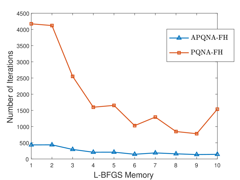
(b) mnist (d=782, m=100000)

(c) connect-4 (d=126, m=10000)

(d) HAPT (d=561, m=7767)

Figure 1: APQNA-FH vs. PQNA-FH in terms of number of iterations.

(a) a9a (d=123, m=32561)

(b) mnist (d=782, m=100000)

(c) connect-4 (d=126, m=10000)

(d) HAPT (d=561, m=7767)

Figure 2: APQNA-FH vs. PQNA-FH in terms of number of function evaluations.

Next, we compare the performance of APQNA-FH versus APQNA-LBFGS to compare the effect of using the fixed approximate Hessian $H_{k}=\frac{1}{\sigma_{k}}H$, which satisfies condition $\sigma_{k}H_{k}\preceq\sigma_{k-1}H_{k-1}$ versus using variable Hessian estimates computed via L-BFGS method at each iteration, while relaxing condition $\sigma_{k}H_{k}\preceq\sigma_{k-1}H_{k-1}$. Table 3 shows the results of this comparison, obtained based on the best choices of memory size for L-BFGS, in particular $\bar{k}=8$ and $\bar{k}=9$, respectively. As we can see, these two algorithms are competitive both in terms of the number of iterations and also the total solution time. Since APQNA-FH does not use the local information of function $f$ to approximate $H_{k}$, it often takes more iterations than APQNA-LBFGS, which constantly updates $H_{k}$ matrices. On the other hand, since APQNA-FH does not require additional computational effort to evaluate $H_{k}$, hence one iteration of this algorithm is cheaper than one iteration of APQNA-LBFGS, which causes the competitive total solution time.

Table 3: APQNA-FH vs. PQNA-LBFGS in terms of function value (Fval), number of iterations (iter) and total solution time (time) in seconds.

a9a
Algorithm	iter	Fval	iter	Fval	iter	Fval	time
APQNA-LBFGS	20	3.4760e-01	40	3.4703e-01	64	3.4703e-01	2.83e+00
APQNA-FH	20	3.4763e-01	40	3.4704e-01	99	3.4703e-01	4.33e+00
mnist
Algorithm	iter	Fval	iter	Fval	iter	Fval	time
APQNA-LBFGS	50	8.9713e-02	100	8.9695e-02	148	8.9695e-02	1.04e+02
APQNA-FH	50	8.9797e-02	100	8.9698e-02	160	8.9695e-02	1.15e+02
connect-4
Algorithm	iter	Fval	iter	Fval	iter	Fval	time
APQNA-LBFGS	30	3.7769e-01	60	3.7688e-01	144	3.7682e-01	8.35e+00
APQNA-FH	30	3.7689e-01	60	3.7682e-01	93	3.7682e-01	3.95e+00
HAPT
Algorithm	iter	Fval	iter	Fval	iter	Fval	time
APQNA-LBFGS	120	7.1860e-02	240	7.1519e-02	356	7.1511e-02	1.04e+02
APQNA-FH	120	7.2134e-02	240	7.1523e-02	376	7.1511e-02	6.89e+01

Finally, we compare APQNA-LBFGS and PQNA-LBFGS, to demonstrate the effect of using an accelerated scheme in the quasi-Newton type proximal algorithms. The results of this comparison are shown in Figure 3 and Figure 4 in terms of the number of iterations and the number of function evaluations, respectively, for different memory sizes of L-BFGS Hessian approximation.

(a) a9a (d=123, m=32561)

(b) mnist (d=782, m=100000)

(c) connect-4 (d=126, m=10000)

(d) HAPT (d=561, m=7767)

Figure 3: APQNA-LBFGS vs. PQNA-LBFGS in terms of number of iterations.

(a) a9a (d=123, m=32561)

(b) mnist (d=782, m=100000)

(c) connect-4 (d=126, m=10000)

(d) HAPT (d=561, m=7767)

Figure 4: APQNA-LBFGS vs. PQNA-LBFGS in terms of number of function evaluations.

Clearly, as we can see in Figure 3 and 4, not only does the accelerated scheme not achieve practical acceleration compared to PQNA-LBFGS in terms of the number of iterations, but it is also inferior in terms of the number of function evaluations, since every iteration requires two function evaluations. Thus, we believe that the practical experiments support our theoretical analysis in that applying acceleration scheme in the case of variable Hessian estimates may not result in a faster algorithm.

6 Conclusion

In this paper, we established a linear convergence rate of PQNA proposed in tang under a strong convexity assumption. To our knowledge, this is the first such result, for proximal quasi-Newton type methods, which have lately been popular in the literature. We also show that this convergence rate is preserved when subproblems are solved inexactly. We provide a simple and practical rule for the number of inner iterations that guarantee sufficient accuracy of subproblem solutions. Moreover, we allow a relaxed sufficient decrease condition during backtracking, which preserves the convergence rate, while it is known to improve the practical performance of the algorithm.

Furthermore, we presented a variant of APQNA as an extension of PQNA. We have shown that this algorithm has the convergence rate of $\mathcal{O}({1}/{k^{2}})$ under a strong condition on the Hessian estimates, which can not always be guaranteed in practice. We have shown that this condition holds when Hessian estimates are a multiple of a fixed matrix, which is computationally less expensive than the more common methods, such as the L-BFGS scheme. Although, this proposed algorithm has the same rate of convergence as the classic APGA, it is significantly faster in terms of the final number of iterations and also the total solution time. Based on the theory, using L-BFGS Hessian approximation, may result in worse convergence rate, however, our computational results show that the practical performance is about the same as that while the fixed matrix. On the other hand, although in these two algorithms, we are applying the accelerated scheme, their practical performances are inferior to that of PQNA-LBFGS, which does not use any accelerated scheme and potentially has a slower sublinear rate of convergence in the absence of strong convexity. We conclude that using variable Hessian estimates is the most efficient approach, and will result in the linear convergence rate in the presence of strong convexity, but that a standard accelerated scheme is not useful in this setting. Exploring other possibly more effective accelerated schemes for the proximal quasi-Newton methods is the subject of future research.

References

- [1] A. Beck and M. Teboulle. A fast iterative shrinkage-thresholding algorithm for linear inverse problems. SIAM, 2:183–202, 2009.
- [2] R. Byrd, J. Nocedal, and F. Oztoprak. An inexact successive quadratic approximation method for convex -regularized optimization. Technical Report, 2013.
- [3] R. H Byrd, J. Nocedal, and R. B Schnabel. Representations of quasi Newton matrices and their use in limited memory methods. Mathematical Programming, 63:129–156, 1994.
- [4] D. Drusvyatskiy and A. S. Lewis. Error bounds, quadratic growth, and linear convergence of proximal methods. Technical Report, 2011.
- [5] H. Ghanbari and K. Scheinberg. Optimization algorithms in machine learning. Doctoral Dissertation, 2016.
- [6] C. J. Hsieh, M. Sustik, I. Dhilon, and P. Ravikumar. Sparse inverse covariance matrix estimation using quadratic approximation. NIPS, pages 2330–2338, 2011.
- [7] K. Jiang, D. Sun, and K. Toh. An inexact accelerated proximal gradient method for large scale linearly constrained convex SDP. SIAM, 22:1042–1064, 2012.
- [8] J. D. Lee, Y. Sun, and M. A. Saunders. Proximal Newton-type methods for convex optimization. Technical Report, 2012.
- [9] A. Nemirovski and D. Yudin. Informational complexity and efficient methods for solution of convex extremal problems. J. Wiley and Sons, New York, 1983.
- [10] Y. E. Nesterov. A method for solving the convex programming problem with convergence rate . Soviet Mathematics Doklady, 27:372–376, 1983.
- [11] Y. E. Nesterov. Introductory Lectures on Convex Programming: A Basic Course. Springer, 2004.
- [12] Y. E. Nesterov. Smooth minimization for non-smooth functions. Mathematical Programming, 103:127–152, 2005.
- [13] Y. E. Nesterov. Gradient methods for minimizing composite objective function. Mathematical Programming, 140:125–161, 2013.
- [14] J. Nocedal and S.J. Wright. Numerical Optimization. Springer Series in Operations Research. Springer, New York, NY, USA, 2nd edition, 2006.
- [15] P. A. Olsen, F. Oztoprak, J. Nocedal, and S. J. Rennie. Newton-like methods for sparse inverse covariance estimation. NIPS, pages 764–772, 2012.
- [16] P. Richtarik and M. Takac. Iteration complexity of randomized block-coordinate descent methods for minimizing a composite function. Mathematical Programming, 144:1–38, 2014.
- [17] K. Scheinberg, D. Goldfarb, and X. Bai. Fast first-order methods for composite convex optimization with backtracking. Foundation of Mathematics, 14:389–417, 2014.
- [18] K. Scheinberg and I. Rish. A greedy coordinate ascent method for sparse inverse covariance selection problem. SINCO, Technical Report, 2009.
- [19] K. Scheinberg and X. Tang. Practical inexact proximal quasi-Newton method with global complexity analysis. Mathematical Programming, 160:495–529, 2016.
- [20] M. Schmidt, N. L. Roux, and F. Bach. Convergence rate of inexact proximal-gradient method for convex optimization. NIPS, pages 1458–1466, 2011.
- [21] M. Schmidt, N. L. Roux, and F. Bach. Supplementary material for the paper convergence rates of inexact proximal-gradient methods for convex optimization. NIPS, 2011.
- [22] S. Shalev-Shwartz and A. Tewari. Stochastic methods for regularized loss minimization. ICML, pages 929–936, 2009.
- [23] S. Sra, S. Nowozin, and S.J. Wright. Optimization for Machine Learning. Mit Pr, 2011.
- [24] R. Tibshirani. Regression shrinkage and selection via the lasso. Journal of the Royal Statistical Society, Series B, Methodological, 58:267–288, 1996.
- [25] P. Tseng. On accelerated proximal gradient methods for convex-concave optimization. Technical Report, 2008.
- [26] S. Villa, S. Salzo, L. Baldassarre, and A. Verri. Accelerated and inexact forward-backward algorithms. SIAM, 23:1607–1633, 2011.
- [27] G. X. Yuan, K. W. Chang, C. J. Hsieh, and C. J. Lin. A comparison of optimization methods and software for large-scale -regularized linear classification. JMLR, 11:3183–3234, 2010.