¹¹institutetext: Harvard-Smithsonian Center for Astrophysics, MS-3, 60 Garden Street, Cambridge, MA 02138, USA ²²institutetext: Department of Physics and Astronomy, University of Leicester, Leicester LE1 7RH, United Kingdom ³³institutetext: Max-Planck-Institut für Extraterrestrische Physik, Giessenbachstraße , 85748 Garching, Germany ⁴⁴institutetext: MIT Kavli Institute for Astrophysics and Space Research, Cambridge, MA 02139, ⁵⁵institutetext: University of Sheffield, Department of Physics and Astronomy, Hounsfield Road, Sheffield S3 7RH, United Kingdom

SNR 1E 0102.2-7219 as an X-ray Calibration Standard in the 0.5–1.0 keV Bandpass and Its Application to the CCD Instruments aboard Chandra, Suzaku, Swift and XMM-Newton

Paul P. Plucinsky 11 Andrew P. Beardmore 22 Adam Foster 11 Frank Haberl 33 Eric D. Miller 44 A.M.T. Pollock 55 Steve Sembay 22

(Received 3 May 2016 / Accepted 30 June 2016)

Abstract

Context. The flight calibration of the spectral response of CCD instruments below 1.5 keV is difficult in general because of the lack of strong lines in the on-board calibration sources typically available. This calibration is also a function of time due to the effects of radiation damage on the CCDs and/or the accumulation of a contamination layer on the filters or CCDs.

Aims. We desire a simple comparison of the absolute effective areas of the current generation of CCD instruments onboard the following observatories: Chandra ACIS-S3, XMM-Newton (EPIC-MOS and EPIC-pn), Suzaku XIS, and Swift XRT and a straightforward comparison of the time-dependent response of these instruments across their respective mission lifetimes.

Methods. We have been using 1E 0102.2-7219, the brightest supernova remnant in the Small Magellanic Cloud, to evaluate and modify the response models of these instruments. 1E 0102.2-7219 has strong lines of O, Ne, and Mg below 1.5 keV and little or no Fe emission to complicate the spectrum. The spectrum of 1E 0102.2-7219 has been well-characterized using the RGS gratings instrument on XMM-Newton and the HETG gratings instrument on Chandra. As part of the activities of the International Astronomical Consortium for High Energy Calibration (IACHEC), we have developed a standard spectral model for 1E 0102.2-7219 and fit this model to the spectra extracted from the CCD instruments. The model is empirical in that it includes Gaussians for the identified lines, an absorption component in the Galaxy, another absorption component in the SMC, and two thermal continuum components with different temperatures. In our fits, the model is highly constrained in that only the normalizations of the four brightest lines/line complexes (the O vii He $\alpha$ triplet, O viii Ly $\alpha$ line, the Ne ix He $\alpha$ triplet, and the Ne x Ly $\alpha$ line) and an overall normalization are allowed to vary, while all other components are fixed. We adopted this approach to provide a straightforward comparison of the measured line fluxes at these four energies. We have examined these measured line fluxes as a function of time for each instrument after applying the most recent calibrations that account for the time-dependent response of each instrument.

Results. We perform our effective area comparison with representative, early mission data when the radiation damage and contamination layers were at a minimum, except for the XMM-Newton EPIC-pn instrument which is stable in time. We find that the measured fluxes of the O vii He $\alpha$ r line, the O viii Ly $\alpha$ line, the Ne ix He $\alpha$ r line, and the Ne X Ly $\alpha$ line generally agree to within $\pm 10\%$ for all instruments, with 38 of our 48 fitted normalizations within $\pm 10\%$ of the IACHEC model value. We then fit all available observations of 1E 0102.2-7219 for the CCD instruments close to the on-axis position to characterize the time dependence in the 0.5–1.0 keV band. We present the measured line normalizations as a function of time for each CCD instrument so that the users may estimate the uncertainty in their measured line fluxes for the epoch of their observations.

Key Words.:

instrumentation: detectors — X-rays: individual: 1E 0102.2-7219 — ISM: supernova remnants — X-rays: ISM — Stars: supernovae: general

1 Introduction

This paper reports the progress of a working group within the International Astronomical Consortium for High Energy Calibration (IACHEC) to develop a calibration standard for X-ray astronomy in the bandpass from 0.3 to 1.5 keV. An introduction to the IACHEC organization, its objectives and meetings, may be found at the web page http://web.mit.edu/iachec/. Our working group was tasked with selecting celestial sources with line-rich spectra in the 0.3–1.5 keV bandpass which would be suitable cross-calibration targets for the current generation of X-ray observatories. The desire for strong lines in this bandpass stems from the fact that the quantum efficiency and spectral resolution of the current CCD-based instruments is changing rapidly from 0.3 to 1.5 keV but the on-board calibration sources currently in use typically have strong lines at only two energies, 1.5 keV (Al K $\alpha$ ) and 5.9 keV (Mn K $\alpha$ ). The only option available to the current generation of flight instruments to calibrate possible time variable responses in this bandpass is to use celestial sources. The missions which have been represented in this work are the Chandra X-ray Observatory (Chandra) (Weisskopf et al., 2000, 2002), the X-ray Multimirror Mission (XMM-Newton) (Jansen et al., 2001), the ASTRO-E2 Observatory (Suzaku), and the Swift Gamma-ray Burst Mission (Swift) (Gehrels et al., 2004). Data from the following instruments have been included in this analysis: the High-Energy Transmission Grating (HETG) (Canizares et al., 2005) and the Advanced CCD Imaging Spectrometer (ACIS) (Bautz et al., 1998; Garmire et al., 2003, 1992) on Chandra, the Reflection Gratings Spectrometers (RGS) (den Herder et al., 2001), the European Photon Imaging Camera (EPIC) Metal-Oxide Semiconductor (EPIC-MOS) (Turner et al., 2001) CCDs and the EPIC p-n junction (EPIC-pn) (Strüder et al., 2001) CCDs on XMM-Newton, the X-ray Imaging Spectrometer (XIS) on Suzaku, and the X-ray Telescope (XRT) (Burrows et al., 2005; Godet et al., 2007) on Swift.

Ideal calibration targets would need to possess the following qualities. The source would need to be constant in time, to have a simple spectrum defined by a few bright lines with a minimum of line-blending, and to be extended so that “pileup” effects in the CCDs are minimized but not so extended that the off-axis response of the telescope dominates the uncertainties in the response. Our working group focused on supernova remnants (SNRs) with thermal spectra and without a central source such as a pulsar, as the class of source which had the greatest likelihood of satisfying these criteria. We narrowed our list to the Galactic SNR Cas A, the Large Magellanic Cloud remnant N132D and the Small Magellanic Cloud remnant 1E 0102.2-7219 (hereafter E0102). We discarded Cas A since it is relatively young ( $\sim 350$ yr), with significant brightness fluctuations in the X-ray, radio, and optical over the past three decades (Patnaude & Fesen, 2007, 2009; Patnaude et al., 2011), it contains a faint (but apparently variable) central source, and it is relatively large (radius $\sim 3.5$ arcminutes). We discarded N132D because it has a complicated, irregular morphology in X-rays (Borkowski et al., 2007) and its spectrum shows strong, complex Fe emission (Behar et al., 2001). The spectrum of N132D is significantly more complicated in the 0.5–1.0 keV bandpass than the spectrum of E0102. We therefore settled on E0102 as the most suitable source given its relatively uniform morphology, small size (radius $\sim 0.4$ arcminutes), and comparatively simple X-ray spectrum.

We presented preliminary results from this effort in Plucinsky et al. (2008) and Plucinsky et al. (2012) using a few observations with the calibrations available at that time. In this paper, we present an updated analysis of the representative data acquired early in the various missions and expand our investigations to include a characterization of the time dependence of the response of the various CCD instruments. The low energy responses of some of the instruments (ACIS-S3, EPIC-MOS, & XIS) included in this analysis have a complicated time dependence due to the time-variable accumulation of a contamination layer. A primary objective of this paper is to inform the Guest Observer communities of the respective missions on the current accuracy of the calibration at these low energies.

2 The SNR 1E 0102.2-7219

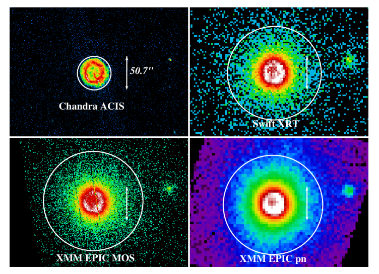
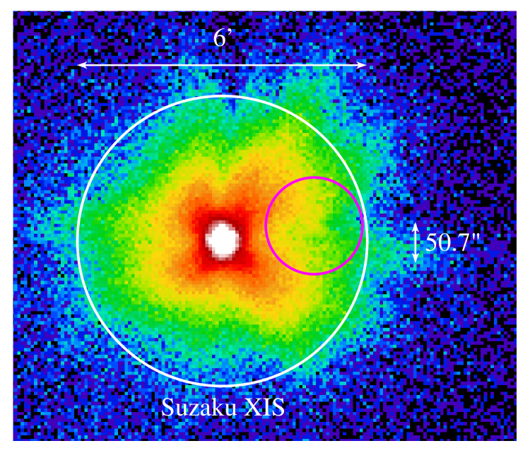
The SNR E0102 was discovered by the Einstein Observatory (Seward & Mitchell, 1981). It is the brightest SNR in X-rays in the Small Magellanic Cloud (SMC). E0102 has been extensively imaged by Chandra (Gaetz et al., 2000; Hughes et al., 2000) and XMM-Newton (Sasaki et al., 2001). Figures 1 and 2 show images of E0102 with the relevant spectral extraction regions for each of the instruments included in this analysis. E0102 is classified as an “O-rich” SNR based on the optical spectra acquired soon after the X-ray discovery (Dopita et al., 1981) and confirmed by followup observations (Tuohy & Dopita, 1983). The age was estimated as $\sim 1,000$ yr by Hughes et al. (2000) based on the expansion deduced from comparing Chandra images to ROSAT images, but Finkelstein et al. (2006) estimate an age of $\sim 2,050$ yr based on twelve filaments observed during two epochs by the Hubble Space Telescope (HST). Blair et al. (1989) presented the first UV spectra of E0102 and argued for a progenitor mass between 15 and 25 $M_{\odot}$ based on the derived O, Ne, and Mg abundances. Blair et al. (2000) refined this argument with Wide Field and Planetary Camera 2 and Faint Object Spectrograh data from HST to suggest that the precursor was a Wolf-Rayet star of between 25 and 35 $M_{\odot}$ with a large O mantle that produced a Type Ib supernova. Sasaki et al. (2006) compared the UV spectra from the Far Ultraviolet Spectroscopic Explorer to the CCD spectra from XMM-Newton to conclude that a single ionization timescale cannot fit the O, Ne, and Mg emission lines, possibly indicating a highly structured ejecta distribution in which the O, Ne, and Mg have been shocked at different times. Vogt & Dopita (2010) argued for an asymmetric, bipolar structure in the ejecta based on spectroscopy of the [O III] filaments. The Spitzer Infrared Spectrograph detected strong lines of O and Ne in the infrared (IR) (Rho et al., 2009). In summary, all available spectral data in the optical, UV, IR, and X-ray bands indicate significant emission from O, Ne, & Mg with very little or no emission from Fe or other high Z elements.

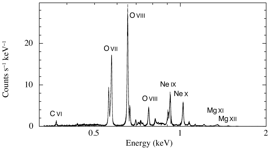
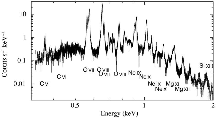
The diameter of E0102 is small enough such that a high resolution spectrum may be acquired with the HETG on Chandra and the RGS on XMM-Newton. The HETG spectrum (Flanagan et al., 2004) and the RGS spectrum (Rasmussen et al., 2001) both show strong lines of O, Ne, and Mg with little or no Fe, consistent with the spectra at other wavelengths. E0102’s spectrum is relatively simple compared to a typical SNR spectrum. Figure 3 displays the RGS spectrum from E0102. The strong, well-separated lines in the energy range 0.5 to 1.5 keV make this source a useful calibration target for CCD instruments with moderate spectral resolution in this bandpass. The source is extended enough to reduce the effects of photon pileup, which distorts a spectrum. Although some pileup is expected in all the non-grating instruments when observed in modes with relatively long frame times. The source is also bright enough to provide a large number of counts in a relatively short observation. Given these characteristics, E0102 has become a standard calibration source that is observed repeatedly by all of the current generation of X-ray observatories.

Refer to caption — Figure 1: Images of E0102 from ACIS-S3 (top left), EPIC-MOS (bottom left), XRT (top right), EPIC-pn (bottom right). The white circles indicate the extraction regions used for the spectral analysis. The fine structure in E0102 is evident in the Chandra image. Note that the Chandra extraction region is the smallest.

3 Spectral Modeling and Fitting

3.1 Construction of The Spectral Model

Our objective was to develop a model which would be useful in calibrating and comparing the response of the CCD instruments; therefore, the model presented here is of limited value for understanding E0102 as a SNR. Our approach was to rely upon the high-resolution spectral data from the RGS and HETG to identify and characterize the bright lines and the continuum in the energy range from 0.3–2.0 keV and the moderate-spectral resolution data from the EPIC-MOS and EPIC-pn to characterize the lines and continuum above 2.0 keV. Since our objective is calibration, we decided against using any of the available plasma emission models for several reasons. First, the Chandra results on E0102 (Flanagan et al., 2004; Gaetz et al., 2000; Hughes et al., 2000) have shown there are significant spectral variations with position in the SNR, implying that the plasma conditions are varying throughout the remnant. Since the other missions considered here have poorer angular resolution than Chandra, the emission from these regions is mixed such that the unambiguous interpretation of the fitted parameters of a plasma emission model is difficult if not impossible. Second, the available parameter space in the more complex codes is large, making it difficult to converge on a single best fit which represents the spectrum. We therefore decided to construct a simple, empirical model based on interstellar absorption components, Gaussians for the line emission, and continuum components which would be appropriate for our limited calibration objectives.

We assumed a two component absorption model using the tbabs (Wilms et al., 2000) model in XSPEC. The first component was held fixed at $5.36\times 10^{20}\leavevmode\nobreak\ {\mathrm{c}m^{-2}}$ to account for absorption in the Galaxy. The second component was allowed to vary in total column, but with the abundances fixed to the lower abundances of the SMC (Russell & Bessell, 1989; Russell & Dopita, 1990, 1992). We modeled the continuum using a modified version of the APEC plasma emission model (Smith et al., 2001) called the ‘‘No-Line’’ model. This model excludes all line emission, while retaining all continuum processes including bremsstrahlung, radiative recombination continua (RRC), and the two-photon continuum from hydrogenic and helium-like ions (from the strictly forbidden ${}^{2}S_{1/2}2s\rightarrow$ gnd and ${}^{1}S_{0}1s2s\rightarrow$ gnd transitions, respectively). Although the bremsstrahlung continuum dominates the X-ray spectrum in most bands and at most temperatures, the RRCs can produce observable edges while the two-photon emission creates ’bumps’ in specific energy ranges. The ‘‘No-Line’’ model assumes collisional equilibrium and so may overestimate the RRC edges in an ionizing plasma or have the wrong total flux in some of the two-photon continua. However, the available data did not justify the use of a more complex model, while the simpler bremsstrahlung-only model showed residuals in the RGS spectra that were strongly suggestive of RRC edges. The RGS data were adequately fit by a single continuum component, but the HETG, EPIC-MOS, and EPIC-pn data showed an excess at energies above 2.0 keV. We therefore added a second continuum component to account for this emission.

The lines were modeled as simple Gaussians in XSPEC. The lines were identified in the RGS and HETG data in a hierarchical manner, starting with the brightest lines and working down to the fainter lines. We have used the ATOMDB v2.0.2 (Foster et al., 2012) database to identify the transitions which produce the observed lines. The RGS spectrum from 23 observations totaling 708/680 ks for RGS1/RGS2 is shown in Fig. 3(top) with a linear Y axis to emphasize the brightest lines. The spectrum is dominated by the O vii He $\alpha$ triplet at 560-574 eV, the O viii Ly $\alpha$ line at 654 eV, the Ne ix He $\alpha$ triplet at 905-922 eV, and the Ne X Ly $\alpha$ line at 1022 eV. This figure demonstrates the lack of strong Fe emission in the spectrum of E0102. The identification of the lines obviously becomes more difficult as the lines become weaker. Figure 3(bottom) shows the same spectrum but with a logarithmic Y axis. In this figure, one is able to see the weaker lines more clearly and also the shape of the continuum. Lines were added to the spectrum at the known energies for the dominant elements, C, N, O, Ne, Mg, Si, S, and Fe and the resulting decrease in the reduced $\chi^{2}$ value was evaluated to determine if the addition of the line was significant. The list of lines identified in the RGS and HETG data were checked for consistency. The identified lines were compared against representative spectra from the vpshock model (with lines) to ensure that no strong lines were missed.

In this manner a list of lines in the 0.3–2.0 keV bandpass was developed based upon the RGS and HETG data. In addition, the temperature and normalization were determined for the low-temperature APEC ‘‘No-Line’’ continuum component. These model components were then frozen and the model compared to the EPIC-pn, EPIC-MOS, and XIS data. Weak lines above 2.0 keV were evident in the EPIC-pn, EPIC-MOS, and XIS data and also what appeared to be an additional continuum component above 2.0 keV. Several lines were added above 2.0 kev and a high-temperature continuum component with kT $\sim 1.7$ keV was added. Once the model components above 2.0 keV had been determined, the RGS data were re-fit with components above 2.0 keV frozen to these values and the final values for the SMC $N_{\mathrm{H}}$ and the low-temperature continuum were determined. In practice, this was an iterative process which required several iterations in fitting the RGS and EPIC-MOS/EPIC-pn/XIS data. Once the absorption and continuum components were determined, the parameters for those components were frozen and the final parameters for the line emission were determined from the RGS data. We included 52 lines in the final model and these lines are described in Table 1. When fitting the RGS data, the line energies were allowed to vary by up to 1.0 eV from the expected energy to account for the shifts when an extended source is observed by the RGS. Shifts of less than 1.0 eV are too small to be significant when fitting the CCD instrument data. The line widths were also allowed to vary. In most cases the line widths are small but non-zero, consistent with the Doppler widths seen in the RGS (Rasmussen et al., 2001) and HETG (Flanagan et al., 2004) data, $\sigma_{E}\approx 0.003\times E$ ; but in a few cases noted in the table the widths are larger than this value. This is most likely due to weak, nearby lines which our model has ignored. We do not have an identification for the line-like feature at 1.4317 keV, but we note that it is weak.

As noted above, the identification of the lines becomes less certain as the line fluxes get weaker. Our primary purpose is to characterize the flux in the bright lines of O and Ne. Any identification of a line with flux less than $1.0\times 10^{-4}\leavevmode\nobreak\ {\mathrm{photons\leavevmode\nobreak\ cm^{-2}\leavevmode\nobreak\ s^{-1}}}$ in Table 1 should be considered tentative. The Fe lines in Table 1 warrant special discussion. There are nine Fe lines included in our model from different ions. We have not verified the self-consistency of the Fe lines included in this model. As our objective is calibration and not the characterization of the plasma that might produce these Fe lines, the possible lack of consistency does not affect our analysis. Of particular note is the Fe XIX line at 917 eV with zero flux. We went through several iterations of the model with this line included and excluded. Unfortunately this line is only 2 eV away from the Ne ix He $\alpha$ i line at 915 eV and neither the RGS nor the HETG has the resolution to separate lines this close together. We have decided to attribute all the flux in this region to the Ne IX He $\alpha$ i line but have retained the Fe XIX line for future investigations. It is possible that some of the emission which we have identified as Fe emission is due to other elements. For our calibration objective this is not important because all of the Fe lines are weak and they do not have a significant effect on the fitted parameters of the bright lines of O and Ne. We hope that future instruments will have the resolution and sensitivity to uniquely identify the weak lines in the E0102 spectrum.

Table 1: Spectral Lines Included in the E0102 Reference Model (v1.9)

Line ID	E (keV) ^a	$\lambda$ (Å) ^a	Flux ^b	Line ID	E (keV) ^a	$\lambda$ (Å) ^a	Flux ^b
C VI Ly $\alpha$	0.3675	33.737	175.2	Ne IX He $\alpha$ i	0.9148	13.553	249.6
Fe XXIV	0.3826	32.405	18.4	Fe XIX	0.9172	13.517	0.0
S XIV	0.4075	30.425	11.8	Ne IX He $\alpha$ r	0.922	13.447	1380.5
N VI He $\alpha$ f	0.4198	29.534	6.8	Fe XX	0.9668 ^c	12.824	120.5
N VI He $\alpha$ i	0.4264	29.076	2.0	Ne X Ly $\alpha$	1.0217	12.135	1378.3
N VI He $\alpha$ r	0.4307	28.786	10.5	Fe XXIII	1.0564	11.736	24.2
C VI Ly $\beta$	0.4356	28.462	49.5	Ne IX He $\beta$	1.074	11.544	320.7
C VI Ly $\gamma$	0.4594	26.988	27.3	Ne IX He $\gamma$	1.127	11.001	123.1
O VII He $\alpha$ f	0.561	22.1	1313.2	Fe XXIV	1.168 ^c	10.615	173.5
O VII He $\alpha$ i	0.5686	21.805	494.4	Ne X Ly $\beta$	1.211	10.238	202.2
O VII He $\alpha$ r	0.5739	21.603	2744.7	Ne X Ly $\gamma$	1.277	9.709	78.5
O VIII Ly $\alpha$	0.6536	18.969	4393.3	Ne X Ly $\delta$	1.308	9.478	37.1
O VII He $\beta$	0.6656	18.627	500.9	Mg XI He $\alpha$ f	1.3311	9.314	108.7
O VII He $\gamma$	0.6978	17.767	236.1	Mg XI He $\alpha$ i	1.3431	9.231	27.5
O VII He $\delta$	0.7127	17.396	124.9	Mg XI He $\alpha$ r	1.3522	9.169	231.0
Fe XVII	0.7252	17.096	130.9	?	1.4317	8.659	8.1
Fe XVII	0.7271 ^c	17.051	165.9	Mg XII Ly $\alpha$	1.4721	8.422	110.2
Fe XVII	0.7389	16.779	82.3	Mg XI He $\beta$	1.579 ^c	7.852	50.6
O VIII Ly $\beta$	0.7746	16.006	788.6	Mg XI He $\gamma$	1.659	7.473	16.0
Fe XVII	0.8124 ^c	15.261	90.5	Mg XII Ly $\beta$	1.745 ^c	7.105	29.7
O VIII Ly $\gamma$	0.817	15.175	243.1	Si XIII He $\alpha$ f	1.8395	6.74	13.8
Fe XVII	0.8258	15.013	65.1	Si XIII He $\alpha$ i	1.8538	6.688	3.4
O VIII Ly $\delta$	0.8365	14.821	62.7	Si XIII He $\alpha$ r	1.865	6.647	34.6
Fe XVIII	0.8503 ^c	14.581	407.3	Si XIV Ly $\alpha$	2.0052	6.183	11.2
Fe XVIII	0.8726 ^c	14.208	89.6	Si XIII He $\beta$	2.1818	5.682	4.3
Ne IX He $\alpha$ f	0.9051	13.698	690.2	S XV He $\alpha$ f,i,r	2.45	5.06	12.7

^a Theoretical rest energies; wavelengths are $hc/E$ .

^b Flux in $10^{-6}$ photons cm^-2 s^-1

^c This line is broader than the nominal width, see text

3.2 Fitting Methodology

The spectral data were fit using the XSPEC software package (Arnaud et al., 1999) with the modified Levenberg-Marquardt minimization algorithm and the C statistic (Cash, 1979) as the fitting statistic. We fit the data in the energy range from 0.3–2.0 keV since that is the energy range in which E0102 dominates over the background. We adopted the C statistic as the fitting statistic to avoid the well-known bias with the $\chi^{2}$ statistic with a low number of counts per bin (see Cash, 1979; Nousek & Shue, 1989) and the bias that persists even with a relatively large number of counts per bin (see Humphrey et al., 2009). Given how bright E0102 is compared to the typical instrumental background, the low number of counts per bin bias should only affect the lowest and highest energies in the 0.3–2.0 keV bandpass. The EPIC-pn spectra were fit with both the C statistic and the $\chi^{2}$ statistic and the derived parameters were nearly identical. The EPIC-pn spectra have the largest number of counts and the count rate is stable in time over the mission. We performed the final fits for the EPIC-pn with $\chi^{2}$ as the fit statistic. The source extraction regions for each of the CCD instruments are shown in Figures 1 & 2. The source and background spectra were not binned in order to preserve the maximal spectral information. Suitable backgrounds were selected for each instrument nearby E0102 where there was no obvious enhancement in the local diffuse emission. If the C statistic is used and the user does not supply an explicit background model, XSPEC computes a background model based on the background spectrum provided in place of a user-provided background model. XSPEC does not subtract the background spectrum from the source spectrum in this case, rather the source and background spectra are both modeled. This is referred to in the XSPEC documentation as the so-called “W statistic” ¹¹1see https://heasarc.gsfc.nasa.gov/xanadu/xspec/manual/
qXSappendixStatistics.html. Although this approach is suitable for our analysis objectives, it may not be suitable if the source is comparable to or only slightly brighter than the background. In such a case, it might be beneficial to specify an explicit background model with its own free parameters and fit simultaneously with the source spectral model. Given how bright the O vii He $\alpha$ triplet, O viii Ly $\alpha$ line, the Ne ix He $\alpha$ triplet, and the Ne x Ly $\alpha$ line are compared to the background, our determination of these line fluxes is rather insensitive to the background modeling method.

Some of the spectral data sets for the various instruments showed evidence of gain variations from one observation to another. Our analysis method is sensitive to shifts in the gain since our model spectrum has strong, well-separated lines and the line energies are frozen in our fitting process. These gain shifts could be due to a number of factors such as uncertainties in the bias or offset calculation at the beginning of the observation, drifts in the gain of the electronics, or variable particle background. Since our objective is to determine the most accurate normalization for a line at a known energy, it is important that the line be well-fitted. We experimented with the gainfit command in XSPEC for the data sets that showed evidence of a possible gain shift and determined that the fits to the lines improved significantly in some cases. One disadvantage of the gainfit approach is that the value of the effective area is then evaluated at a different energy and this introduces a systematic error in the determination of the line normalization. We determined that for gain shifts of 5 eV or less, the error introduced in the derived line normalization is less than 2% which is typically smaller than our statistical uncertainty on a line normalization from a single observation. The gain shifts for the EPIC-MOS and EPIC-pn spectra were small enough that gainfit could be used. The gain shifts for ACIS-S3, XIS, and XRT could be larger for some observations, on the order of $\pm 10$ eV. Therefore, we adopted the approach of applying the indicated gain shift to the event data outside of XSPEC, re-extracting the spectra from the modified events lists, and then fitting the modified spectrum to determine the normalization of the line. The ACIS-S3, XIS, & XRT data had gain shifts applied to their data in this manner.

The number of free parameters needed to be significantly reduced before fitting the CCD data in order to reduce the possible parameter space. In our fits, we have frozen the line energies and widths, the SMC $N_{\mathrm{H}}$ , and the low-temperature APEC ‘‘No-Line’’ continuum to the RGS-determined values. The high-temperature APEC ‘‘No-Line’’ component was frozen at the values determined from the EPIC-pn and EPIC-MOS. The fixed absorption and continuum components are listed in Table 2. Since the CCD instruments lack the spectral resolution to resolve lines which are as close to each other as the ones in the O vii He $\alpha$ triplet and the Ne ix He $\alpha$ triplet, we treated nearby lines from the same ion as a “line complex” by constraining the ratios of the line normalizations to be those determined by the RGS and by constraining the line energies to the known separations. In practice, we would typically link the normalization and energy of the f and i lines of the triplet to the r line (except for O vii for which we linked the other lines to the f line). Since we also usually freeze the energies of the lines, this means that the three lines in the triplet would have only one free parameter, the normalization of the Resonance line. We have constructed the model in XSPEC such that it would be easy to vary the energy of the r line in the triplet (and hence also the f and i) to examine the gain calibration of a detector at these energies. Our philosophy is to treat nearby lines as a complex which can adjust together in normalization and energy. In this paper, we focus on adjusting the normalization of the line complexes only. Since most of the power in the spectrum is in the bright line complexes, we froze all the normalizations of the weaker lines. The only normalizations which we allowed to vary were the O vii He $\alpha$ f, O viii Ly $\alpha$ line, the Ne ix He $\alpha$ r, and the Ne X Ly $\alpha$ line normalizations. In addition, we found it useful to introduce a constant scaling factor of the entire model to account for the fact that the extraction regions for the various instruments were not identical. In this manner, we restricted a model with more than 200 parameters to have only 5 free parameters in our fits. The final version of this model in the XSPEC .xcm file format is available on the IAHCEC web site, on the Thermal SNRs Working Group page: https://wikis.mit.edu/confluence/display/iachec/Thermal+SNR. We will refer to this at the IACHEC standard model for E0102 or the “IAHCEC model.”

Table 2: Fixed Absorption and Continuum Components

Model Component	Value
Galactic absorption	$N_{\mathrm{H}}$ $=5.36\times 10^{20}\leavevmode\nobreak\ {\rm cm^{-2}}$
SMC absorption	$N_{\mathrm{H}}$ $=5.76\times 10^{20}\leavevmode\nobreak\ {\rm cm^{-2}}$
APEC ‘‘No-Line’’ temperature #1	kT=0.164 keV
APEC ‘‘No-Line’’ normalization #1	$3.48\times 10^{-2}\leavevmode\nobreak\ {\rm cm^{-5}}$
APEC ‘‘No-Line’’ temperature #2	kT=1.736 keV
APEC ‘‘No-Line’’ normalization #2	$1.85\times 10^{-3}\leavevmode\nobreak\ {\rm cm^{-5}}$

4 Observations

E0102 has been routinely observed by Chandra, Suzaku, Swift, and XMM-Newton, as a calibration target to monitor the response at energies below 1.5 keV. The IACHEC standard model was developed using primarily RGS and HETG data as described in Sect. 3.1. We include a description of the RGS and HETG data in this section for completeness, but our primary objective is to improve the calibration of the CCD instruments. Therefore, the RGS and HETG data were analyzed with the calibration available at the time the model was finalized. We continue to update the processing and analysis of the CCD instrument data as new software and calibration files become available. For this paper, we have selected a subset of these CCD instrument observations for the comparison of the absolute effective areas. We have selected data from the timeframe and the instrument mode for which we are the most confident in the calibration and used those data in this comparison. We have also analyzed all available E0102 data from a given instrument in the same mode, close to on-axis in order to characterize the time dependence of the response of the individual instruments. We now describe the data processing and calibration issues for each instrument individually.

4.1 XMM-Newton RGS

4.1.1 Instruments

XMM-Newton has two essentially identical high-resolution dispersive grating spectrometers, RGS1 and RGS2, that share telescope mirrors with the EPIC instruments MOS1 and MOS2 and operate between 6 and 38 Å or 0.3 and 2.0 keV. The size of its 9 CCD detectors along the Rowland circle define apertures of about 5 arcminutes within which E0102 fits comfortably. Each CCD has an image area of $1024\times 384$ pixels, integrated on the chip into bins of $3\times 3$ pixels. The data consist of individual events whose wavelengths are determined by the grating dispersion angles calculated from the spatial positions at which they were detected. Overlapping orders are separated through the event energies assigned by the CCDs. The RGS instruments have suffered the build-up of a contamination layer of carbon included automatically in the calibration. The status of the RGS calibration is summarized in de Vries et al. (2015). Built-in redundancies have ensured complete spectral coverage despite the loss early in the mission of one CCD detector each in RGS1 and RGS2.

4.1.2 Data

E0102 has been a regular XMM-Newton calibration source with over 30 observations (see Table 3) made at initially irregular intervals and variety of position angles between 2000 April 16 and 2011 November 04. All of these data have been used in the analysis reported here using spectra calculated on a fixed wavelength grid by SAS v11.0.0 separately as normal for RGS1 and RGS2 and for 1st and 2nd orders. An initial set of 23 observations before the end of 2007 was combined using the SAS task rgscombine to give spectra of high statistical weight with exposure times of 708080 s for RGS1 and 680290 s for RGS2 and used at an early stage to define the IACHEC model discussed above.

Table 3: XMM RGS Observations of E0102

rev	ObsID	DATE	Exposure(ks)
0065	0123110201	2000-04-16	22.7
0065	0123110301	2000-04-17	21.7
0247	0135720601	2001-04-14	33.5
0375	0135720801	2001-12-25	35.0
0433	0135720901	2002-04-20	35.7
0447	0135721001	2002-05-18	34.1
0521	0135721101	2002-10-13	27.2
0552	0135721301	2002-12-14	29.0
0616	0135721401	2003-04-20	45.5
0711	0135721501	2003-10-27	30.5
0721	0135721701	2003-11-16	27.4
0803	0135721901	2004-04-28	35.2
0888	0135722401	2004-10-14	31.1
0894	0135722001	2004-10-26	31.9
0900	0135722101	2004-11-06	49.8
0900	0135722201	2004-11-07	31.9
0900	0135722301	2004-11-07	31.9
0981	0135722501	2005-04-17	37.1
1082	0135722601	2005-11-05	30.4
1165	0135722701	2006-04-20	30.5
1265	0412980101	2006-11-05	32.4
1351	0412980201	2007-04-25	36.4
1443	0412980301	2007-10-26	37.1
1531	0412980501	2008-04-19	29.9
1636	0412980701	2008-11-14	28.9
1711	0412980801	2009-04-13	28.9
1807	0412980901	2009-10-21	28.9
1898	0412981001	2010-04-21	30.5
1989	0412981301	2010-10-18	32.0
2081	0412981401	2011-04-20	35.1
2180	0412981501	2011-11-04	30.2

Table 4: ACIS and ACIS/HETG Observations of E0102

OBSID	Instrument	DATE	Exposure	Counts^a𝑎a^a𝑎a $a$ Counts for ”ACIS-HETG” are the sum of MEG $\pm 1$ order events, $0.5-2$ keV.	Mode
			(ks)	(0.5-2.0 keV)
112120^b𝑏b^b𝑏b $b$ Observation included in the comparison of effective areas discussed in Section 5.3.	ACIS-HETG	1999-09-28	187.9	138917	TE, Faint, 3.2 s frametime
112968^b𝑏b^b𝑏b $b$ Observation included in the comparison of effective areas discussed in Section 5.3.	ACIS-HETG	1999-10-08	148.4	122566	TE, Faint, 3.2 s frametime
123828^b𝑏b^b𝑏b $b$ Observation included in the comparison of effective areas discussed in Section 5.3.	ACIS-HETG	2002-12-20	135.9	149599	TE, Faint, 3.2 s frametime
12147	ACIS-HETG	2011-02-11	148.9	144341	TE, Faint, 3.2 s frametime
123545^b𝑏b^b𝑏b $b$ Observation included in the comparison of effective areas discussed in Section 5.3.	ACIS-S3	2003-08-08	127.9	157111	TE, 1/4 subarray, 1.1 s frametime, node 1
126765^b𝑏b^b𝑏b $b$ Observation included in the comparison of effective areas discussed in Section 5.3.	ACIS-S3	2006-03-19	127.6	151745	TE, 1/4 subarray, 0.8 s frametime, node 0
18365	ACIS-S3	2007-02-11	121.0	138685	TE, 1/4 subarray, 0.8 s frametime, node 0
19694	ACIS-S3	2008-02-07	119.2	124795	TE, 1/4 subarray, 0.8 s frametime, node 0
10654	ACIS-S3	2009-03-01	127.3	145534	TE, 1/4 subarray, 0.8 s frametime, node 0
10655	ACIS-S3	2009-03-01	126.8	143227	TE, 1/8 subarray, 0.4 s frametime, node 0
10656	ACIS-S3	2009-03-06	127.8	148601	TE, 1/4 subarray, 0.8 s frametime, node 1
11957	ACIS-S3	2009-12-30	118.5	112423	TE, 1/4 subarray, 0.8 s frametime, node 0
13093	ACIS-S3	2011-02-01	119.1	108286	TE, 1/4 subarray, 0.8 s frametime, node 0
14258	ACIS-S3	2012-01-12	119.1	102048	TE, 1/4 subarray, 0.8 s frametime, node 0
15467	ACIS-S3	2013-01-28	119.1	192610	TE, 1/4 subarray, 0.8 s frametime, node 0
16589	ACIS-S3	2014-03-27	129.6	140194	TE, 1/4 subarray, 0.8 s frametime, node 0
17380	ACIS-S3	2015-02-28	117.7	165809	TE, 1/4 subarray, 0.8 s frametime, node 0
17688	ACIS-S3	2015-07-17	129.6	133972	TE, 1/4 subarray, 0.8 s frametime, node 0

²²2

4.1.3 Processing

As E0102 is an extended source, it required special treatment with SAS v11.0.0 whose usual procedures are designed for the analysis of point sources. This simply involved the definition of custom rectangular source and background regions taking into account both the size of the SNR and the cross-dispersion instrumental response caused by scattering from the gratings. In cross-dispersion angle from the SNR centre, the source regions were $\pm 0.75^{\prime}$ and the background regions were between $\pm 1.42^{\prime}$ and $\pm 2.58^{\prime}$ . An individual measurement was thus encapsulated in a pair of simultaneous spectra, one combining source and background, the other the background only.

4.2 Chandra HETG

4.2.1 Instruments

The HETG is one of two transmission gratings on Chandra which can be inserted into the converging X-ray beam just behind the High Resolution Mirror Assembly (HRMA). When this is done the resulting HRMA–HETG–ACIS-S configuration is the high-energy transmission grating spectrometer (HETGS, often used interchangeably with just HETG). The HETG and its operation are described as a part of Chandra (Weisskopf et al., 2000, 2002) and in HETG-specific publications (Canizares et al., 2000, 2005).

The HETG consists of two distinct sets of gratings, the medium-energy gratings (MEGs) and the high-energy-gratings (HEGs) each of which produces plus– and minus– order dispersed spectral images with the dispersion angle nearly proportional to the photon wavelength. The result is that a point source produces a non-dispersed “zeroth-order” image (the same as if the HETG were not inserted, though with reduced throughput) as well as four distinct linear spectra forming the four arms of a shallow “X” pattern on the ACIS-S readout; see Fig. 1 of both Canizares et al. (2000) & Canizares et al. (2005).

Hence, an HETG observation yields four first-order spectra, the MEG $\pm$ 1 orders and the HEG $\pm$ 1 orders ³³3There are also higher-valued orders, $m=2,3,$ …, but their throughput is much below the first-orders’; the most useful of these are the MEG $\pm$ 3 and the HEG $\pm 2$ orders each with $\sim$ $\times$ 0.1 the throughput of the first orders.. Because the dispersed photons are spread out and detected along the ACIS-S, the calibration of the HETG involves more than a single ACIS CCD: the minus side orders fall on ACIS CCDs S2, S1, and S0, while the plus side orders are on S3, S4, and S5. Hence the calibration of all ACIS-S CCDs is important for the HETG calibration.

When the object observed with the HETG is not a point source, the dispersed images become something like a convolution of the spatial and spectral distributions of the source; see Dewey (2002) for a brief elaboration of these issues. The upshot is that for the extended-source case the response matrix function (rmf) of the spectrometer is determined by the spatial characteristics of the source and the position angle of the dispersion direction on the sky, set by the observation roll angle. These considerations guide the HETG analyses that follow.

4.2.2 Data

E0102 was observed as part of the HETG GTO program at three epochs (see Table 4).: Sept.–Oct. 1999 (obsids 120 & 968, $t=$ 1999.75, exp $=$ 88.2 $+$ 49.0 ks, roll $=$ 11.7^∘), in December of 2002 (obsid 3828, $t=$ 2002.97, exp $=$ 137.7 ks, roll $=$ 114.0+180^∘), and most recently in February of 2011 (obsid 12147, $t=$ 2001.11, exp $=$ 150.8 ks, roll $=$ 56.5+180^∘). The roll angles of these epochs were deliberately chosen to differ with a view toward future spectral-tomographic analyses. The HETG view of E0102 is presented in Flanagan et al. (2004) using the first epoch observations: the bright ring of E0102 is dispersed and shows multiple ring-like images due to the prominent emission lines in the spectrum. The combination of all three epoch’s MEG data is shown in Fig. 4.

In principle, one can analyze the 2D spectral images directly (Dewey, 2002) to get the most information from the data. This involves doing forward-folding of spatial-spectral models to create simulated 2D images which are compared with the data (Dewey & Noble, 2009). The lower image of Fig. 4 shows such a simulated model for the combined MEG data sets based on the observed E0102 zeroth-order events, the IACHEC standard model, and CIAO-generated ARFs. However, for the limited purpose of fitting the 5-parameter IACHEC model to the HETG data we can collapse the data to 1D and use the standard HETG extraction procedures (next section).

4.2.3 Processing

The first steps in HETG data analysis are the extraction of 1D spectra and the creation of their corresponding ARFs (as mentioned above the point-source RMFs are not applicable to E0102.) Because of differences in the pointing of the two first-epoch observations, they are separately analyzed and so we extract the 4 HETG spectra from each of the 4 obsids available. The archive-retrieved data were processed using TGCat ISIS scripts (Huenemoerder et al., 2011); these provide a useful wrapper to execute the CIAO extraction tools. Several customizations were specified before executing TGCat’s do-it-all run_pipe() command:

•

The extraction center was manually input and chosen to be at the center of a 43 sky-pixel radius circle that approximates the outer blastwave location. For the recent-epoch obsid 12147, this is at RA 01:04:02.11 and Dec -72:01:52.2 (J2000 coordinates.s). This location is 0.5 sky-pixels East and 7 sky-pixels North of the centroid of the bright blob at the inner end of the “Q-stroke” feature. This offset from a feature in the data was used to determine the equivalent center location in the other obsids.
•

The cross-dispersion widths of the MEG and HEG spectral extractions were set to cover a range of $\pm$ 55 sky-pixels about the dispersion axes.
•

The order-sorting limits were explicitly set to a large constant value of $\pm$ 0.20 ⁴⁴4For the first epoch, early in the Chandra mission, the ACIS focal plane temperature was at $-110^{\circ}$ C. For these obsids we used a somewhat larger order-sorting range of $\pm$ 0.25..

Because E0102 covers a large range in the cross-dispersion direction compared with the $\pm$ 16 pixel dither range, we generated for each extraction a set of 7 ARFs spaced to cover the 110 pixels of the cross-dispersion range. In making the ARFs we set osipfile=none because of our large order-sorting limits. Finally, background extractions were made as for the data but with the extraction centers shifted by 120 pixels in the cross-dispersion direction.

The fitting of the HETG extractions generally follows the methodology outlined in Sect. 3.2 with some adjustments because of the extended nature of E0102, and, secondarily, because of the use of the ISIS platform (Houck, 2002). For each obsid and grating–order we read in the extracted source and background spectra (PHA files) and, after binning (below), the background counts are subtracted bin-by-bin from the source counts. The corresponding set of ARFs that span E0102’s cross-dispersion extent are read in, averaged, and assigned to the data. An RMF that approximates the spatial effects of E0102 is created and assigned as well, see Fig. 5. Finally the model is defined in ISIS and its 5 free parameters are fit and their confidence ranges determined.

The ARFs for the HETG contain two general types of features: those that depend on the photon energy, such as mirror reflectivity, grating efficiency and detector QE, and other effects that depend on the specific location on the readout array where the photon is detected, such as bad pixels and chip gaps. For a point source there is very nearly a one-to-one mapping of photon energy and location of detection, hence the two terms are combined in the overall ARF, the SPECRESP values in the FITS file. The latter term is, however, available separately via the FRACEXPO values and this is used to remove the location-specific contribution from the ARF. The RMF is made in-software using ISIS’s load_slang_rmf() routine. The resulting RMF approximates the 1D projected shape of E0102 and appropriately includes the FRACEXPO features.

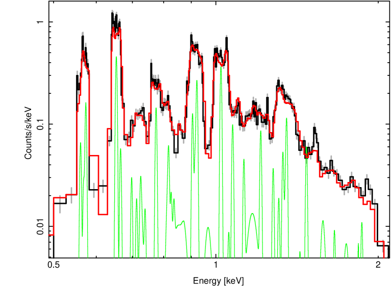
As shown in Fig. 5, the HETG 1D extracted spectra are reasonably approximated by the model folded through the approximate-RMF. However, because the RMF is not completely accurate, we reduce its influence on the fitting by defining a coarse binning of 10 bins from 0.54 to 2.0 keV (23 – 6.2 Å). The boundaries of the bins are chosen to be between the brightest lines, and the three lowest-energy bins are not used when fitting an HEG spectrum.

4.3 XMM-Newton EPIC-pn

4.3.1 Instruments

The EPIC-pn instrument is based on a back-illuminated $6\times 6$ cm² monolithic X-ray CCD array covering the 0.15–12 keV energy band. Four individual quadrants each having three EPIC-pn-CCD subunits with a format of $200\times 64$ pixels are operated in parallel covering a $\sim$ 13 $\aas@@fstack{\prime}$ 6 $\times$ 4 $\aas@@fstack{\prime}$ 4 rectangular region. Different CCD-readout modes are available which allow faster readout of restricted CCD areas, with frame times from 73 ms for the full-frame (FF), 48 ms for large-window (LW), and 6 ms for the small window (SW) mode, the fastest imaging mode (Strüder et al., 2001).

4.3.2 Data

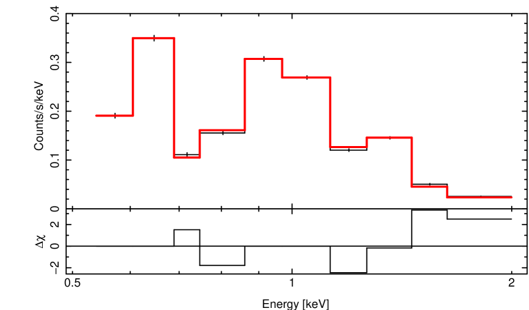
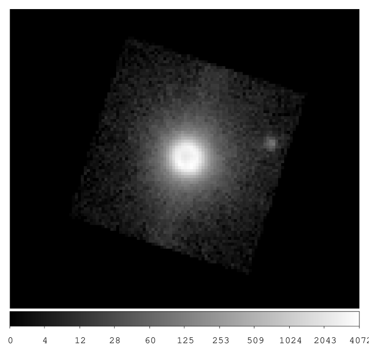
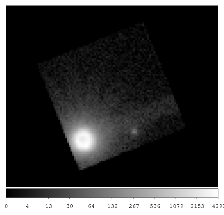
XMM-Newton observed E0102 with EPIC-pn in all imaging readout modes (FF, LW and SW) and all available optical blocking filters. To rule out photon pile-up effects we only used spectra from SW mode data for our analysis. Between 2001-12-25 and 2015-10-30 (satellite revolution 375 to 2910) E0102 was observed by XMM-Newton with EPIC-pn in small window (SW) mode 24 times (see Table LABEL:tab-obs-epicpn). Two observations were performed with the thick filter while for 11 (11) observations the thin (medium) filter was used. One set of observations placed the source at the nominal boresight position which is close to a border of the $4.4\arcmin\times 4.4\arcmin$ read-out window of EPIC-pn-CCD 4 and therefore only a relatively small extraction radius of 30″ is possible. During 14 observations the source was centered in the SW area which allows an extraction with 75″ radius. For comparison we show in Fig. 6 the images binned to $4\arcsec\times 4\arcsec$ pixels from observation 0135720801 (with the SNR centered) and 0412981401 (nominal target position).

4.3.3 Processing

The data were processed with XMM-NewtonSAS version 14.0.0 and we extracted spectra using single-pixel events (PATTERN=0 and FLAG=0) to obtain highest spectral resolution. Response files were generated using rmfgen and arfgen, assuming a point source for PSF corrections. Due to the extent of E0102, the standard PSF correction for the lost flux outside the extraction region introduces systematic errors, leading to different fluxes from spectra using different extraction radii. To utilize the observations with the target placed at the nominal boresight position, we extracted spectra from the SW-centered observations with 30″ and 75″ radius. For the large extraction radius, PSF losses are negligible and, from a comparison of the two spectra, an average correction factor 1.0315 was derived to account for the PSF losses in the smaller extraction region.

In order to derive reliable line fluxes from the EPIC-pn spectra, the lines must be at their nominal energies as accurately as possible. Otherwise, the high statistical quality leads to bad fits and wrong line normalisations. Energy shifts of generally less than 5 eV in the EPIC-pn spectra of E0102 lead to increases in $\chi^{2}$ from typical values of 600-700 to 700-800 and changes in line normalisations by $\sim 2$ %. Only for the highest required gain shifts of 7–8 eV (Fig. 7) errors in the line normalisations reach $\sim 5$ %. Therefore, we created for each observation a set of event files with the energies of the events (the PI value) shifted by up to $\pm$ 9 eV in steps of 1 eV. In order to do so the initial event file was produced with an accuracy of 1 eV for the PI values (PI values are stored as integer numbers with an accuracy of 5 eV by default) using the switch testenergywidth=yes in epchain. Spectra were then created from the 19 event files with the standard 5 eV binning. The 19 spectra from each of the SW mode observations were fitted using the model described in Sect. 3.1 with five free parameters (the overall normalisation factor and 4 line normalisations representing the O VII He $\alpha$ f, O VIII Ly $\alpha$ , Ne IX He $\alpha$ r and Ne X Ly $\alpha$ ). The best-fit spectrum was then used to obtain the energy adjustment and the line normalisations for each observation. In parallel we determined the energy adjustment using the gain fit command in XSPEC with the standard spectrum, only allowing the shift as free parameter and fixing the slope to 1.0. A comparison of the required energy adjustments obtained from the two methods shows no significant differences. Therefore, we proceeded to use the gain fit in XSPEC because it is simpler to use.

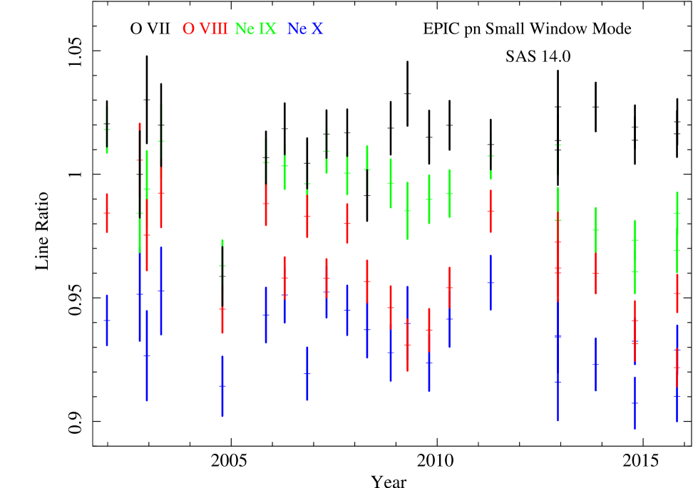
In Fig. 7 we show the derived energy shift (using gain fit) for the SW mode observation as function of time. No clear trend is visible with an average shift of $+1.8\pm 1.0$ eV (1 $\sigma$ confidence), which is well within the instrument channel width of 5 eV. However, a systematic difference between the two sets of observations (boresight, centered) is revealed. For the observations with the target placed at boresight (centered) the average shift was determined to $-0.7\pm 0.5$ eV ( $+3.6\pm 1.2$ eV). The boresight position is the best calibrated which is supported by the small average energy shift. The centre location corresponds to different RAWX and RAWY coordinates on the CCD. It is closer to the CCD read out (lower RAWY) and therefore charge transfer losses are reduced. On the other hand the gain depends on the read-out column (RAWX). Therefore, it is not clear if uncertainties in the gain or charge transfer calibration or both are responsible for the difference in energy scale of about 4 eV at the two positions. Similar position-dependent effects were found from observations of the isolated neutron star RX J1856.5-3754 (Sartore et al., 2012).

The line normalisations of the four line complexes after the gain fit (multiplied by the overall normalisation and corrected to the large extraction radius) relative to the model normalisations are shown in Fig. 8. For each line complex the derived line normalisations are consistent with being constant in time. The largest deviations are seen from the fifth observation, one for which the thick filter was used. On the other hand, during revolution 2380 (2012-12-06) three observations were performed with the three different filters yielding consistent results. The average values (fitting a constant to the normalisations) are 1.014 $\pm$ 0.004 (O vii), 0.959 $\pm$ 0.003 (O viii), 0.991 $\pm$ 0.003 (Ne ix) and 0.933 $\pm$ 0.004 (Ne x). The O viii and Ne x ratios are significantly lower by about 5% than the ratios from their corresponding lower ionization lines. A possible error in the calibration over such relatively narrow energy bands is difficult to understand and needs further investigation.

4.4 XMM-Newton EPIC-MOS

4.4.1 Instruments

XMM-Newton (Jansen et al., 2001) has three X-ray telescopes each with a European Photon Imaging Camera (EPIC) at the focal plane. Two of the cameras have seven MOS CCDs (henceforth MOS1 and MOS2) (Turner et al., 2001) and the third has twelve pn CCDs (see Sect. 4.3). Apart from the characteristics of the detectors, the telescopes are differentiated by the fact that the MOS1 and MOS2 telescopes contain the reflection grating arrays which direct approximately half the X-ray flux into the apertures of the reflection grating spectrometers (RGS1 and RGS2).

Table 5: MOS Observations of E0102

OBSID	Instrument	DATE	Exposure	Counts	Mode
			(ks)	(0.5-2.0 keV)
0123110201^a𝑎a^a𝑎a $a$ Observation included in the comparison of effective areas discussed in Section 5.3.	MOS1	2000-04-16	17.4	160354	LW, 0.9s frametime, thin filter
0123110201^a𝑎a^a𝑎a $a$ Observation included in the comparison of effective areas discussed in Section 5.3.	MOS2	2000-04-16	17.4	160633	LW, 0.9s frametime, thin filter
0123110301^a𝑎a^a𝑎a $a$ Observation included in the comparison of effective areas discussed in Section 5.3.	MOS1	2000-04-17	12.1	140092	LW, 0.9s frametime, medium filter
0123110301^a𝑎a^a𝑎a $a$ Observation included in the comparison of effective areas discussed in Section 5.3.	MOS2	2000-04-17	12.1	140893	LW, 0.9s frametime, medium filter
0135720601	MOS1	2001-04-14	18.6	165561	LW, 0.9s frametime, thin filter
0135720601	MOS2	2001-04-14	18.6	162927	LW, 0.9s frametime, thin filter
0135720801	MOS1	2001-12-25	28.0	102340	LW, 0.9s frametime, thin filter
0135720801	MOS2	2001-12-25	28.0	199855	LW, 0.9s frametime, thin filter
0135721301	MOS1	2002-12-14	27.2	193882	LW, 0.9s frametime, thin filter
0135721301	MOS2	2002-12-14	27.2	193392	LW, 0.9s frametime, thin filter
0135721501	MOS1	2003-10-27	21.0	176062	LW, 0.9s frametime, thin filter
0135721501	MOS2	2003-10-27	21.0	170285	LW, 0.9s frametime, thin filter
0135721901	MOS1	2004-04-28	31.0	106535	LW, 0.9s frametime, thin filter
0135721901	MOS2	2004-04-28	31.0	104510	LW, 0.9s frametime, thin filter
0135722401	MOS1	2004-10-14	29.4	184006	LW, 0.9s frametime, thick filter
0135722401	MOS2	2004-10-14	29.4	180836	LW, 0.9s frametime, thick filter
0135722501	MOS1	2005-04-17	29.4	198331	LW, 0.9s frametime, thin filter
0135722501	MOS2	2005-04-17	29.4	197993	LW, 0.9s frametime, thin filter
0135722601	MOS1	2005-11-05	29.1	198813	LW, 0.9s frametime, thin filter
0135722601	MOS2	2005-11-05	29.1	196880	LW, 0.9s frametime, thin filter
0412980101	MOS1	2006-11-05	31.0	102286	LW, 0.9s frametime, thin filter
0412980101	MOS2	2006-11-05	31.0	199904	LW, 0.9s frametime, thin filter
0412980301	MOS1	2007-10-26	35.0	119372	LW, 0.9s frametime, thin filter
0412980301	MOS2	2007-10-26	35.0	111364	LW, 0.9s frametime, thin filter
0412981401	MOS1	2011-04-20	30.3	184751	LW, 0.9s frametime, thin filter
0412981401	MOS2	2011-04-20	30.3	100949	LW, 0.9s frametime, thin filter
0412981701	MOS1	2012-12-06	12.8	139780	LW, 0.9s frametime, thin filter
0412981701	MOS2	2012-12-06	12.8	143069	LW, 0.9s frametime, thin filter
0412981701	MOS1	2012-12-06	16.6	147453	LW, 0.9s frametime, medium filter
0412981701	MOS2	2012-12-06	16.6	153615	LW, 0.9s frametime, medium filter
0412982101	MOS1	2013-11-07	31.3	195929	LW, 0.9s frametime, thin filter
0412982101	MOS2	2013-11-07	31.3	198882	LW, 0.9s frametime, thin filter
0412982201	MOS1	2014-10-20	32.8	104184	LW, 0.9s frametime, thin filter
0412982201	MOS2	2014-10-20	32.8	103544	LW, 0.9s frametime, thin filter

⁵⁵5

4.4.2 Data

E0102 was first observed by XMM-Newton quite early in the mission in April 2000 (orbit number 0065). The MOS observations are listed in (Table 5). This first look at the target in orbit 0065 was split into two observations, each approximately 18 ks in duration, with a different choice of optical filter. Observation 0123110201 had the THIN filter and 0123110301 had the MEDIUM filter. Both filters have a 1600 $\AA$ polyimide film with evaporated layers of 400 $\AA$ and 800 $\AA$ respectively of Aluminum. The EPIC-MOS readout was configured to the Large Window (LW) imaging mode (in the central CCD only the inner $300\times 300$ pixels of the total available $600\times 600$ pixels are read out). LW mode is the most common imaging mode used in EPIC-MOS observations of this target as the faster readout (0.9 s compared with 2.6 s in full frame (FF) mode) minimises pile-up whilst retaining enough active area to contain the whole remnant for pointings up to around 2 arcminutes from the centre of the target. This is useful for exploring the response of the instrument for off-axis angles near to the boresight.

4.4.3 Processing

The EPIC-MOS data were first processed into calibrated event lists with SAS version 12.0.0 and the current calibration files (CCFs) as of May 2013 and later with SAS version 13.5.0 and the CCFs as of December 2013. The signficant differences between the SAS and CCF versions are dealt with in Sect. 5.4.1.

Source spectra were extracted from a circular region of radius 80″ centered on the remnant. Background spectra were taken from source-free regions on the same CCD. The event selection filter in the nomenclature of the SAS was (PATTERN==0)&&(#XMMEA_EM). This selects only mono-pixel events and removes events whose reconstructed energy is suspect due, for example, to proximity to known bright pixels or CCD boundaries which can be noisy.

Mono-pixel events are chosen over the complete X-ray pattern library because it minimises the effects of pile-up with little loss of sensitivity over the energy range of interest. The effects of pile-up on the mono-pixel spectrum can be shown to be small. The mono-pixel pile-up fraction, the fraction of events lost to higher patterns or formed from two (or more) X-rays detected in the same pixel within a frame (the former is more likely by a factor of about 8:1), can be estimated from the observed fraction of diagonal bi-pixel events which arise almost exclusively from the pile-up of two mono-pixel events. By default the SAS splits these events (nominally pattern classes 26 to 29) back into two separate mono-pixels although this action can be switched off. Less than 1.0% of events within the source spectra are diagonal bi-pixels which is approximately the same fraction of mono-pixel events lost to horizontal or vertical bi-pixels (event pattern classes 1 to 4).

We employ a simple screening algorithm to detect flares in the background due to soft protons. Light curves of bin size 100s were created from events with energies greater than 10 keV within the whole aperture. Good time intervals were formed where the observed rate was less than $\rm 0.4\ cts\ s^{-1}$ . The cut-off limit was chosen by manual inspection of the light curves. Typically after this procedure the observed background is less than 1% of the total count rate below 2.0 keV.

All spectra were extracted with a 5.0 eV bin size. Response (RMF) files were generated with the SAS task rmfgen in the energy range of interest with an energy bin size of 1.0 eV. This is comparable to the accuracy with which line centroids can be determined for the stronger lines in this source for typical exposures in the EPIC-MOS. Although the source is an extended, but compact, object, the effective area (ARF) file was calculated with the SAS task arfgen assuming a point-source function model with the switch PSFMODEL=ELLBETA.

Table 6: EPIC-MOS fitting results

Without Gain Fit
	MOS1		MOS2
Parameter^a𝑎a^a𝑎a $a$ Line normalisations for O VII, O VIII, Ne IX and Ne X are multiplied by $10^{-3}$	Thin	Medium	Thin	Medium
Global	1.063 (0.009)	1.057 (0.011)	1.091 (0.009)	1.059 (0.011)
O VII	1.380 (0.026)	1.428 (0.032)	1.385 (0.026)	1.460 (0.033)
O VIII	4.576 (0.068)	4.459 (0.081)	4.487 (0.068)	4.623 (0.085)
Ne IX	1.375 (0.022)	1.369 (0.026)	1.348 (0.022)	1.404 (0.027)
Ne X	1.393 (0.025)	1.371 (0.029)	1.373 (0.025)	1.419 (0.031)
C-stat/dof	450.5/334	413.9/334	432.3/334	419.6/334
With Gain Fit
Global	1.060 (0.009)	1.044 (0.011)	1.081 (0.009)	1.059 (0.011)
O VII	1.383 (0.026)	1.410 (0.032)	1.383 (0.027)	1.449 (0.034)
O VIII	4.609 (0.069)	4.508 (0.082)	4.536 (0.069)	4.650 (0.086)
Ne IX	1.386 (0.022)	1.378 (0.026)	1.361 (0.022)	1.409 (0.027)
Ne X	1.400 (0.026)	1.383 (0.029)	1.385 (0.025)	1.426 (0.031)
Offset	-4.358	-6.293	-6.297	-3.641
Slope	1.0061	1.0059	1.0081	1.0035
C-stat/dof	422.7/332	376.9/332	387.8/332	408.7/332

⁶⁶6

We justify this over attempting to accurately account for the extended nature of the object in the generation of the ARF because to do so is mathematically much more complex and the end result can be predicted to produce a result which would be much closer to the point-source approximation than the basic uncertainties in the calibration. To formally account for the extended nature of the object would require deconvolving the image with the telescope point-spread function to get the true input spatial distribution relative to the mirror and then estimating for each point in the image both the encircled energy fraction (EEF) relative to the applied spectral extraction region and also the vignetting function. The final ARF would then be a counts weighted average of the ARF derived at each point.

As the remnant is approximately a ring like structure $25^{\prime\prime}$ in radius then the bulk of the input photons have an angular distance relative to the circular $80^{\prime\prime}$ extraction region which varies between $55^{\prime\prime}$ to $105^{\prime\prime}$ , but has a mean of about $82^{\prime\prime}$ . The EEF for a point source is approximately 91%, 94% and 96% at $55"$ , $80^{\prime\prime}$ and $105^{\prime\prime}$ respectively (in the energy range of interest). Hence, the adoption of a single EEF for an $80^{\prime\prime}$ radius is estimated to be approximately within 1% of the value that would be derived if one adopted the technically more accurate method outlined previously. Similarly, the calibrated vignetting variation across the remnant is less than 1% hence assuming the representative value at the centre is a justifiable approximation. Overall, the accuracy of the calculated ARF is clearly dominated more by the absolute uncertainty in the calibration of the vignetting and EEF than the point-source assumption employed here.

Fitting of the model to the source spectra followed the recipe described earlier. Table 6 shows the fitting results from each of the EPIC-MOS observations from Orbit 0065. The Thin and Medium filter results are consistent within the errors and the global results for MOS1 and MOS2 (see Sect. 5.3) are the weighted averages of results from each filter. Shifts in the calibration of the event energy scale were investigated using the gain fit command in XSPEC with an improvement in the fit statistic arising from shifts of around $\sim 5$ eV at 1.0 keV. This is typical of the calibration accuracy of the event energy scale in the EPIC-MOS detectors. The values of the parameter normalisations are relatively insensitive to gain shifts of this magnitude. This was confirmed by applying a reverse gain shift, using the values indicated by XSPEC, to the calibrated energies of each event, then re-extracting and re-fitting the spectra.

EPIC-MOS differs from other instruments in this paper because we explicitly use the source model described here to constrain the redistribution model of our RMF. Within a few years of launch it was noticed that the redistribution properties of the central CCD (in both MOS1 and MOS2) in a spatial region centered around the telescope boresight (within $\sim 1$ arcminute) were evolving with time. The change was consistent with an evolution of the strength and shape of the low-energy charge-loss component of the redistribution profile. As we do not have a physical model of this effect accurate enough to describe the changing RMF, it is calibrated using a method of varying the parameters of a phenomenological model of the RMF to provide a best fit solution to a joint simultaneous fit to spectra from our onboard calibration source and several astrophysical sources, including E0102, using fixed spectral models (Sembay et al., 2011). In the case of the astrophysical sources the input spectral models are derived primarily from the RGS and EPIC-pn. The fitting procedure allows variation in the global normalisation of each spectral model otherwise all parameters within the model are fixed. The consequence of this is that the RMF parameters are driven someway towards a result which gives an energy independent cross-calibration between the EPIC-MOS and RGS. This in part explains why the relative line-to-line normalisations are consistent with the RGS although there is a global offset between the instruments (see Sect. 5.3).

4.5 Chandra ACIS

4.5.1 Instruments

The ACIS is an X-ray imaging-spectrometer consisting of the ACIS-I and ACIS-S CCD arrays. The imaging capability is unprecedented with a half-power diameter (HPD) of $\sim$ 1″ at the on-axis position. We use data from one of the back-illuminated CCDs (ACIS-S3) in the ACIS-S array in this analysis since the majority of imaging data have been collected using this CCD and its response at low energies is significantly higher than the front-illuminated CCDs in the ACIS-I array. There are also more observations of E0102 on S3 than on the I array which allows a better characterization of the time dependence of the response. The ACIS-S3 chip is sensitive in the 0.2–10 keV band. The chip has 1024 $\times$ 1024 pixels covering a 8 $\aas@@fstack{\prime}$ 4 $\times$ 8 $\aas@@fstack{\prime}$ 4 area. The spectral resolution is $\approx 150$ eV in the 0.3–2.0 keV bandpass.

4.5.2 Data

The high angular resolution of Chandra compared to the other observatories is apparent in Fig. 1 as evidenced by the fine structure apparent in this SNR. The majority of the observations of E0102 early in the Chandra mission were executed in full-frame mode with 3.2 s exposures. Unfortunately the bright parts of the ring are significantly piled-up when ACIS is operated in its full-frame mode. In 2003, an observation was conducted in subarray mode that showed the line fluxes were depressed compared to the observations in full-frame mode. In 2005, the Chandra calibration team switched to using subarray modes with readout times of 1.1 s and 0.8 s as the default modes to observe E0102 resulting in a reduction in the pileup level. There have been 14 subarray observations of E0102 on the S3 CCD within one arcminute of the on-axis position, twelve in node 0 and two in node 1 (see Table 4). There are other observations of E0102 on S3 at larger off-axis angles which we exclude from the current comparison to the other instruments close to on-axis. We have selected the two earliest OBSIDs for comparison to the other instruments and discuss the analysis of all 14 observations in §5.3.

4.5.3 Processing

The data were processed with the Chandra X-ray Center(CXC) analysis SW CIAO v4.7 and the CXC calibration database CALDB v4.6.8. We followed the standard CIAO data analysis threads to select good events, reject times of high background, and extract source and background spectra in PI channels. Background spectra were extracted from regions off of the remnant that were specific to each observation since the region of the sky covered varied from observation to observation due to the roll angle of the observation. Response matrices were produced using the standard CIAO tool mkacisrmf with PI channels and auxiliary response files were produced using mkwarf to account for the extended nature of E0102. These tools were called as a Chandra Guest Observer would using the CIAO script specextract.pl.

There are several time-dependent effects which the analysis SW attempts to account for (Plucinsky et al., 2003; Marshall et al., 2004; DePasquale et al., 2004). The most important of these is the efficiency correction for the contaminant on the ACIS optical-blocking filter which significantly reduces the efficiency at energies around the O lines. We chose the earliest two OBSIDs to compare to the other instruments since the contamination layer was thinnest at that time. The analysis SW also corrects for the CTI of the BI CCD (S3), including the time-dependence of the gain. Even with this time-dependent gain correction, some of the observations exhibited residuals around the bright lines that appeared to be due to gain issues. We then fit allowing the gain to vary and noticed that some of the observations had significant improvements in the fits when the gain was allowed to adjust. The adjustments were small, about 5 eV which corresponds to one ADU for S3. We derived a non-linear gain correction using the energies of the O vii He $\alpha$ triplet, the O viii Ly $\alpha$ line, the Ne ix He $\alpha$ triplet & Ne X Ly $\alpha$ line, requiring the gain adjustment to go to zero at 1.5 keV. These gain adjustments were applied to the events lists and spectra were re-extracted from these events lists. The modified spectra were used for subsequent fits. This ensures that the line flux is attributed to the correct energy and the appropriate value of the effective area is used to determine the line normalization.

4.6 Suzaku XIS

4.6.1 Instruments

The XIS is an X-ray imaging-spectrometer equipped with four X-ray CCDs sensitive in the 0.2–12 keV band. One CCD is a back-illuminated (XIS1) device and the others are front-illuminated (XIS0, 2, and 3) devices. The four CCDs are located at the focal plane of four co-aligned X-ray telescopes with a half-power diameter (HPD) of $\sim$ 2 $\aas@@fstack{\prime}$ 0. Each XIS sensor has 1024 $\times$ 1024 pixels and covers a 17 $\aas@@fstack{\prime}$ 8 $\times$ 17 $\aas@@fstack{\prime}$ 8 field of view. The XIS instruments, constructed by MIT Lincoln Laboratories, are very similar in design to the ACIS CCDs aboard Chandra. They are fully described by Koyama et al. (2007). Due to expected degradation in the power supply system, Suzaku lost attitude control in June 2015, and the science mission was declared completed in August 2015.⁷⁷7See http://global.jaxa.jp/press/2015/08/20150826_suzaku.html.

The XIS2 device suffered a putative micro-meteorite hit in November 2006 that rendered two-thirds of its imaging area unusable, and it has been turned off since that point. XIS0 also suffered a micro-meteorite hit in June 2009 that affected one-eighth of the device. Since this region is near the edge of the chip, the device was still used for normal observations until the cessation of science operations in August 2015. The other two CCDs continued to operate normally.

Unlike the ACIS devices, the XIS CCDs possess a charge injection capability whereby a controlled amount of charge can be introduced via a serial register at the top of the array. This injected charge acts to fill CCD traps that cause charge transfer inefficiency (CTI), mitigating the effects of on-orbit radiation damage (Ozawa et al., 2009). In practice, the XIS devices were operated with spaced-row charge injection (SCI) on starting in August 2006. A row of fixed charge is injected every 54 rows; the injected row is masked out on-board, slightly reducing the useful detector area. The level of SCI in the FI chips has been set to about 6 keV for the duration of the mission. The level in the BI chip was initially set to 2 keV to reduce noise at soft energies, however in late 2010 and early 2011 this level was raised to 6 keV.

Table 7: XIS Observations of E0102

OBSID	Instrument	DATE	Exposure	Counts	Mode^b𝑏b^b𝑏b $b$ ’SCI’ stands for spaced-row charge injection.
			(ks)^a𝑎a^a𝑎a $a$ Exposure for XIS is for the filtered event data.	(0.5-2.0 keV)
100014010^c𝑐c^c𝑐c $c$ Observation included in the comparison of effective areas discussed in Section 5.3.	XIS0	2005-08-31	22.1	233078	full window,SCI off
100014010^c𝑐c^c𝑐c $c$ Observation included in the comparison of effective areas discussed in Section 5.3.	XIS1	2005-08-31	22.1	271394	full window,SCI off
100014010^c𝑐c^c𝑐c $c$ Observation included in the comparison of effective areas discussed in Section 5.3.	XIS2	2005-08-31	22.1	233475	full window,SCI off
100014010^c𝑐c^c𝑐c $c$ Observation included in the comparison of effective areas discussed in Section 5.3.	XIS3	2005-08-31	22.1	231569	full window,SCI off
100044010	XIS0	2005-12-17	52.6	270904	full window,SCI off
100044010	XIS1	2005-12-17	94.4	224811	full window,SCI off
100044010	XIS2	2005-12-17	52.6	265054	full window,SCI off
100044010	XIS3	2005-12-17	52.6	258182	full window,SCI off
101005030	XIS0	2006-06-27	21.0	224879	full window,SCI off
101005030	XIS1	2006-06-27	18.5	236029	full window,SCI off
101005030	XIS2	2006-06-27	21.0	221734	full window,SCI off
101005030	XIS3	2006-06-27	18.5	217858	full window,SCI off
102002010	XIS0	2007-06-13	24.0	224632	full window,SCI on
102002010	XIS1	2007-06-13	24.0	240526	full window,SCI on
102002010	XIS3	2007-06-13	24.0	221898	full window,SCI on
103001020	XIS0	2008-06-05	17.5	215843	full window,SCI on
103001020	XIS1	2008-06-05	17.5	228543	full window,SCI on
103001020	XIS3	2008-06-05	17.5	215646	full window,SCI on
104006010	XIS0	2009-06-26	17.4	214915	full window,SCI on
104006010	XIS1	2009-06-26	17.4	227072	full window,SCI on
104006010	XIS3	2009-06-26	17.4	215278	full window,SCI on
105004020	XIS0	2010-06-19	15.5	212629	full window,SCI on
105004020	XIS1	2010-06-19	15.5	224207	full window,SCI on
105004020	XIS3	2010-06-19	15.5	212993	full window,SCI on
106002020	XIS0	2011-06-29	27.4	221361	full window,SCI on
106002020	XIS1	2011-06-29	27.4	244156	full window,SCI on
106002020	XIS3	2011-06-29	27.4	223490	full window,SCI on
107002020	XIS0	2012-06-25	29.6	223722	full window,SCI on
107002020	XIS1	2012-06-25	29.6	245564	full window,SCI on
107002020	XIS3	2012-06-25	29.6	226527	full window,SCI on
108002020	XIS0	2013-06-27	33.1	228615	full window,SCI on
108002020	XIS1	2013-06-27	33.1	256869	full window,SCI on
108002020	XIS3	2013-06-27	33.1	231354	full window,SCI on
109001010	XIS0	2014-04-21	29.6	225982	full window,SCI on
109001010	XIS1	2014-04-21	29.6	248706	full window,SCI on
109001010	XIS3	2014-04-21	29.6	226135	full window,SCI on

⁸⁸8

4.6.2 Data

The XIS observations in this work include representative datasets over the course of the mission. E0102 was a standard calibration source for Suzaku, with 74 separate observations during the life of the mission, including the very first observation when the detector doors were opened. We have chosen eleven observations each taken about one year apart and typically 20–30 ksec in duration. One of these observations was taken shortly after launch on 17 Dec 2005, and is the longest single observation of E0102 with the XIS (94 ksec of clean data from the BI CCD and 50 ksec from each of the FI CCDs). However, these data were taken at a time when the molecular contamination on the optical blocking filters was rapidly accumulating. Since the calibration at this epoch is uncertain, we have chosen an earlier, somewhat shorter observation (31 Aug 2005) to compare to the other instruments. The observations are summarized in Table 7. Three of these observations (in 2005 and 2006) were taken with SCI off, the remainder with SCI on. Observations starting in 2011 were taken with the XIS1 SCI level set to 6 keV. Only three observations have been included for XIS2, which ceased operation in late 2006. Normal, full-window observing mode was used for all analyzed datasets.

4.6.3 Processing

The data were reprocessed to at least v2.7 of the XIS pipeline. In particular, the CTI, charge trail, and gain parameters were applied from v20111018 or later of the makepi CALDB file, which reduced the gain uncertainty to less than 10 eV for all of the observations. Further gain correction was performed during the spectral analysis, in a similar way to Chandra ACIS-S3 and as described in Sect. 3.2.

During the data processing, we found a large variation in the Suzaku pointing accuracy, with an average astrometric offset of 20 arcsec but ranging up to 1.5 arcmin. In the worst case this is quite a bit larger than the published astrometric accuracy of 20 arcsec, although smaller than the PSF of the Suzaku XRT mirrors ( $\sim$ 2 arcmin HPD). Given this pointing error, and the presence of a contaminating point source (RXJ0103.6-7201) projected 2 arcmin from E0102, we corrected the pointing by applying a simple offset in RA and Dec to the attitude data. This offset was calculated from a by-eye comparison of the Suzaku centroids of E0102 (in the 0.4–2 keV band) and RXJ0103.6-7201 (in the 2–7 keV band) to the source locations in a stacked Chandra ACIS-S3 image. The offset for each XIS was determined separately and then averaged to produce the attitude offset for a single observation. From the dispersion of these measurements, we estimate that the RMS uncertainty in the corrected astrometry is 5 arcsec, or about 5 unbinned CCD pixels. We note that this correction is different from the Suzaku XRT thermal wobble, which is corrected in the pipeline⁹⁹9ftp://legacy.gsfc.nasa.gov/suzaku/doc/xrt/suzakumemo-2007-04.pdf; and the attitude control problem which plagued the satellite between Dec 2009 and June 2010, which has not been corrected and effectively produces a smearing of the PSF¹⁰¹⁰10ftp://legacy.gsfc.nasa.gov/suzaku/doc/general/suzakumemo-2010-04.pdf.

Spectra were extracted from a 3 arcmin radius aperture, which would contain 95% of the flux from a point source We excluded a 1 arcmin radius region around RXJ0103.6-7201. Background spectra were extracted from a surrounding annulus encompassing 5.6–7.4 arcmin. The redistribution matrix files (RMFs) were produced with the Suzaku FTOOL xisrmfgen (v20110702), using v20111020 of the CALDB RMF parameters. The ancillary response files (ARFs) were produced with the Monte Carlo ray-tracing FTOOL xissimarfgen (v20101105). The ARF includes absorption due to OBF contamination (Koyama et al. 2007), using v20130813 of the CALDB contamination parameters. To ensure the ARF properly accounted for the partially-resolved extent of the source, a Chandra ACIS-S3 broad-band image of the inner 30 arcsec of E0102 was used as an input source for the ray-tracing.

This X-ray binary RXJ0103.6-7201, projected 2 arcmin from E0102, shows up clearly in Chandra ACIS-S3 observations, and it is well-modeled by a power law with spectral index 0.9 plus a thermal mekal component with kT = 0.15 keV, with a strong correlation between the component normalizations (Haberl & Pietsch 2005). By masking it out in the spectral extraction with a 1 arcmin radius circle, we reduce its contribution by 50%. In the region below 3 keV, we expect E0102 thermal emission to dominate the residual contaminating flux by several orders of magnitude.

4.7 Swift XRT

4.7.1 Instruments

The Swift X-ray Telescope (XRT) comprises a Wolter-I telescope, originally built for JET-X, which focuses X-rays onto an e2v CCD22 detector, similar to the type flown on the XMM-Newton EPIC-MOS instruments (Burrows et al., 2005). The CCD, which was responsive to $\sim 0.25-10.0\thinspace\rm{keV}$ X-rays at launch, has dimensions of $600\times 600$ pixels, giving a $23.6\arcmin\times 23.6\arcmin$ field of view. The mirror has a HPD of $\sim 18\arcsec$ and can provide source localization accurate to better than 2″ (Evans et al., 2009).

Table 8: Swift-XRT observation log. The data reported here were taken under target ID number 50050. The reported rates are from grade 0 events and are not corrected for potential loss of exposure due to the location of the source with respect to the detector bad-columns.

Start Date	Stop Date	Exposure	0.3-1.5 keV rate	Offset
		(ks)	( ${\rm count\,s^{-1}}$ )	(eV)
PC mode :
2005-02-18^a𝑎a^a𝑎a $a$ Observation included in the comparison of effective areas discussed in Section 5.3.	2005-05-22	24.2	0.87	+200
2006-03-11	2006-05-05	28.5	0.81	000
2007-06-08	2007-06-13	20.8	0.73	+400
2007-09-25	2007-10-02	28.4	0.73	-600
2008-10-01	2008-10-04	20.4	0.80	+800
2009-10-18	2009-11-27	20.8	0.74	-600
2010-03-16	2010-09-11	40.0	0.68	-100
2011-03-19	2011-09-14	35.3	0.64	-300
2012-03-09	2012-09-13	35.1	0.70	-800
2013-03-15	2013-10-19	43.1	0.61	-1100
2014-03-13	2014-09-27	49.9	0.73	-1100
WT mode :
2005-02-23^a𝑎a^a𝑎a $a$ Observation included in the comparison of effective areas discussed in Section 5.3.	2005-03-01	25.2	1.09	+100
2006-03-11	2006-04-27	27.4	0.91	-200
2007-06-07	2007-06-20	20.7	0.94	+400
2007-09-30	2007-10-01	15.4	0.95	-100
2008-08-24	2008-10-09	17.3	0.87	+1300
2009-10-15	2009-10-20	22.1	0.98	+400
2010-03-21	2010-09-25	40.1	0.95	-700
2011-03-18	2011-10-15	41.5	0.90	-100
2012-03-10	2012-08-21	38.2	0.90	+400
2013-03-24	2013-10-24	38.5	0.81	+200
2014-03-15	2014-10-14	46.7	0.91	+200

¹¹¹¹11

Since its launch in 2004 November, Swift’s primary science goal has been to rapidly respond to gamma-ray bursts (GRBs) and other targets of opportunity (TOOs). To achieve this, the XRT was designed to operate autonomously, so that it could measure GRB light curves and spectra over several orders of magnitude in flux. In order to mitigate the effects of pile-up, the XRT can automatically switch between different CCD readout modes depending on the source brightness. The two most frequently-used modes are: Windowed Timing (WT) mode, which provides 1D spatial information and spectroscopy in the central 7.8 arcminutes of the CCD with a time resolution of 1.8 ms, and Photon Counting (PC) mode, which allows full 2D imaging-spectroscopy with a time resolution of 2.5 s (see Hill et al., 2004, for further details).

The CCD charge transfer inefficiency (CTI) was seen to increase approximately threefold a year after launch and has steadily worsened since then. The location and depth of the deepest charge traps responsible for the CTI in the central 7.8 arcminutes of the CCD have been monitored since 2007 September and methods have been put in place to minimize their effect on the spectral resolution (Pagani et al., 2011), however, even with such trap corrections, the intrinsic resolution of the CCD has slowly deteriorated with time.

A description of the XRT CCD initial in-flight calibration can be found in Godet et al. (2009). However, since this paper, the XRT spectral calibration has been completely reworked, with both PC and WT RMFs generated from a newly rewritten CCD Monte Carlo simulation code (Beardmore et al., in prep.). The recalibration included a modification to the low energy quantum efficiency (above the oxygen edge at $0.545\thinspace\rm{keV}$ ), in order to improve the modelling of the E0102 line normalisations compared with the IACHEC model for the first epoch XRT WT observation (i.e. 2005; see Sect. 4.7.2).

4.7.2 Data

E0102 is used as a routine calibration source by the Swift-XRT, with $\sim 20$ ks observations taken every 6 to 12 months in both PC and WT mode. The data are used to check the low energy gain calibration of the CCD, as well as to monitor the degradation in energy resolution below $1\thinspace\rm{keV}$ . The observations are performed under target ID 50050.

As Swift has a flexible observing schedule, often interrupted by GRBs or TOOs, observations consist of one or more snapshots on the target, where each snapshot has a typical exposure of $1-2$ ks, assigned to a unique observation identification number (ObsID). When observing E0102, it is necessary to accumulate data from different ObsIDs for any given epoch to build up sufficient statistics in the spectra. We chose to divide the data by year¹²¹²12There are two epochs in 2007 corresponding to observations taken before and after a change made to the CCD substrate voltage. which gives ample temporal resolution for monitoring the CCD spectral response evolution. The observation summary is shown in Table 8. The data were taken over 68 ObsIDs in PC and 61 in WT, with exposures totalling 276.6 ks and 266.4 ks in each mode, respectively.

We select observations taken in 2005 for comparison with the other instruments, as these data were taken when the CCD charge transfer efficiency and spectral resolution were at their best, and the observations took place before a micrometeoroid struck the CCD, introducing bad-columns which make the absolute flux calibration more uncertain. We discuss the results from the following epochs (2006–2013) in Sect. 5.4.4.

4.7.3 Processing

The data were processed with the latest Swift-XRT pipeline software (version 4.3) and CALDB release 2014-Jun-10 was used, which includes the latest epoch dependent RMFs that track the ever broadening response kernel of the CCD. We selected grade 0 events for the spectral comparison, as this minimises the effects of pile-up on the PC mode data. Due to its faster readout, the WT data are free from pile-up. A circular region of radius 30 pixels ( $70.7\arcsec$ ) was used for the spectral extraction for both modes, though due to the 1D nature of the WT readout this effectively becomes a box of size $60\times 600$ pixels (in detector coordinates) in this mode. Background spectra were selected from suitably sized annular regions. The source and background spectra from each ObsID in a particular epoch were then summed. For WT mode, the background is $\sim 10\times$ larger than that in PC mode and dominates the WT source spectrum above $\sim 3\thinspace\rm{keV}$ . (Note, the WT background spectrum BACKSCAL keyword has to be modified to ensure the correct 1D proportional sizes of the extraction regions are used, otherwise insufficient background is subtracted when the spectra are read into XSPEC.)

For PC mode, exposure corrected ancillary response files (ARFs) were created by taking the Chandra ACIS-S3 image (which has a superior spatial resolution to the XRT) and convolving it with the XRT point spread function. Then, by comparing the exposure corrected convolved counts in the extraction region to the total number in the image, an ARF correction factor could be estimated. The ARFs were then corrected for vignetting by supplying the exposure weighted average source offaxis angle position to the xrtmkarf task using the offaxis option.

For WT mode, per snapshot ARFs were created assuming point source corrections can be applied — the convolved Chandra ACIS-S3 image analysis showed that the $70.7\arcsec$ extraction region contains 95 percent of the SNR encircled energy fraction, which is consistent at the $1-2$ percent level to that obtained if it is treated as a point source. However, the latter corrections can become inaccurate (at the 10 percent level) when the remnant is situated on the CCD bad-columns (e.g. for the data taken after 2005). The ancillary response files were then averaged, weighted by the snapshot exposure time.

The spectral gain calibration was checked for energy scale offsets in two ways. First, a gain offset fit was performed in XSPEC when the standard model was applied to the data. In the second method, the data were reprocessed applying offsets in 1 eV steps (i.e. a tenth the size of the nominal PI channel width) and the resulting spectra were then fit to find the one which minimized the C-statistic. Both methods gave consistent results and the measured offsets are reported in Table 8, which shows the energy scale is good to better than $11\thinspace\rm{eV}$ for most epochs. The gain corrected spectra were used in the analysis which follows.

5 Analysis & Results

5.1 Time Variability

E0102 has an estimated age of 1000-2000 yr based on the expansion studies of Hughes et al. (2000) and Finkelstein et al. (2006). It is possible that there might be discernible changes in the integrated X-ray spectrum of a SNR this young over a time span of $\sim 15$ yr. In order to place an upper limit on any changes in the integrated X-ray spectrum, we examined the total count rate from E0102 with the EPIC-pn instrument in the 0.3–2.0 keV band. The EPIC-pn instrument has proven to be the most stable instrument included in our analysis. The total count rate as measured by the EPIC-pn has varied by less than 1.3% over the 14 years of measurements. We conclude that whatever changes might be occurring in E0102, the effect on the integrated X-ray spectrum is small.

We also examined the Chandra images over a 7.5 yr timeframe for differences. The images were exposure-corrected to account for the time-variable absorption of the contamination layer on the ACIS filter and difference images were created. We limited the time span to 7.5 yr to reduce the impact of the uncertainty in the correction for time-variable contamination layer. We calculated the percentage difference between the two observations in narrow bands around the bright emission line complexes of O vii He $\alpha$ , O viii Ly $\alpha$ , Ne ix He $\alpha$ & Ne X Ly $\alpha$ . The largest differences are on the order of 2% in a $0.5\arcsec\times 0.5\arcsec$ pixel. Some parts of the remnant have apparently brightened while other parts have dimmed. The total flux change is consistent with the value measured with the EPIC-pn; however we note that the ACIS-S3 value has a much larger uncertainty given the relatively large correction that must be applied for the contamination layer. An analysis of flux changes on arcsecond spatial scales would require a detailed registration of the Chandra images and is beyond the scope of this paper. It is possible that some of the changes we observe in the difference images at the few percent level are due to a less accurate registration of the images at the two epochs. For the current analysis, we can conclude that the flux in a few arcsecond region might be changing by as much as 2% over a 7.5 yr timespan, but the effect on the integrated spectrum is less than 1.3%.

Table 9: Fit Statistics for Data Sets Included in the Comparison

Instrument	DOF	C Statistic	$\chi^{2}$	reduced $\chi^{2}$
ACIS-S3	227	444.9	463.3	2.04
MOS1	332	415.1	421.6	1.27
MOS2	332	422.9	431.6	1.30
pn	337	761.2	762.7	2.26
XIS0	461	713.8	683.1	1.48
XIS1	461	864.6	898.2	1.99
XIS2	461	742.7	688.6	1.49
XIS3	461	904.6	835.1	1.81
XRT WT mode	106	178.2	178.0	1.68
XRT PC mode	106	140.9	143.4	1.35

5.2 Spectral Fits to the Reference Data

The details of our spectral fitting methodology are described in Sect. 3.2. The key points are that we fit in the 0.3–2.0 keV energy range, we do not subtract background, we do not bin our spectra, and we use the so-called “W statistic” in XSPEC which is a modified version of the C statistic as the fit statistic. The one exception to this is that the $\chi^{2}$ statistic was used for the fits to the EPIC-pn spectra as described in Sect. 3.2. The spectra for each of the CCD instruments were first compared to the IACHEC model without allowing any of the parameters to vary. It was noticed that a global offset to account for different size extraction regions would help to reconcile the overall normalization of the spectra. The spectra were then fit with 5 free parameters: a constant factor multiplying the entire spectrum which acts as a global normalization, and the O vii He $\alpha$ f, O viii Ly $\alpha$ , Ne ix He $\alpha$ r & Ne X Ly $\alpha$ line normalizations. After the best fit had been found by minimizing the C statistic, we freeze the parameters at their best-fit values and compute the $\chi^{2}$ using the model value as the weight instead of the data. We report these $\chi^{2}$ values for readers who might be more accustomed to using the $\chi^{2}$ statistic.

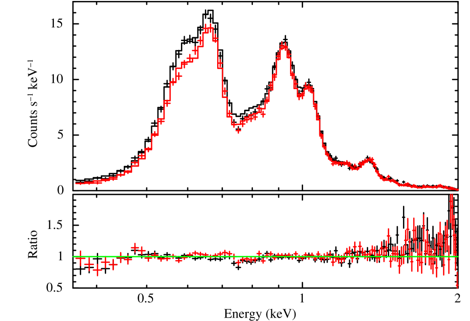
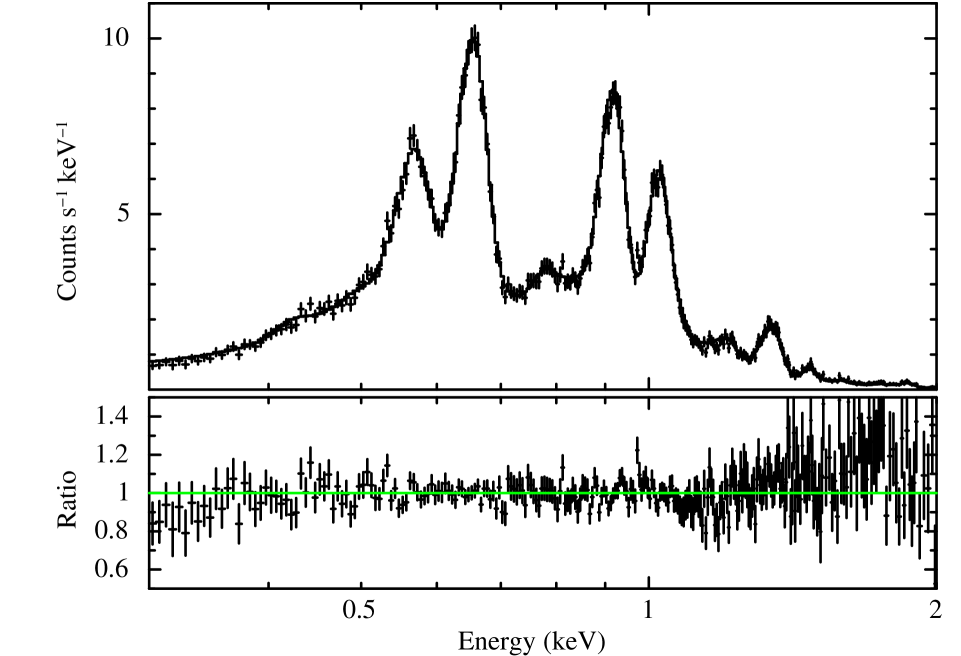
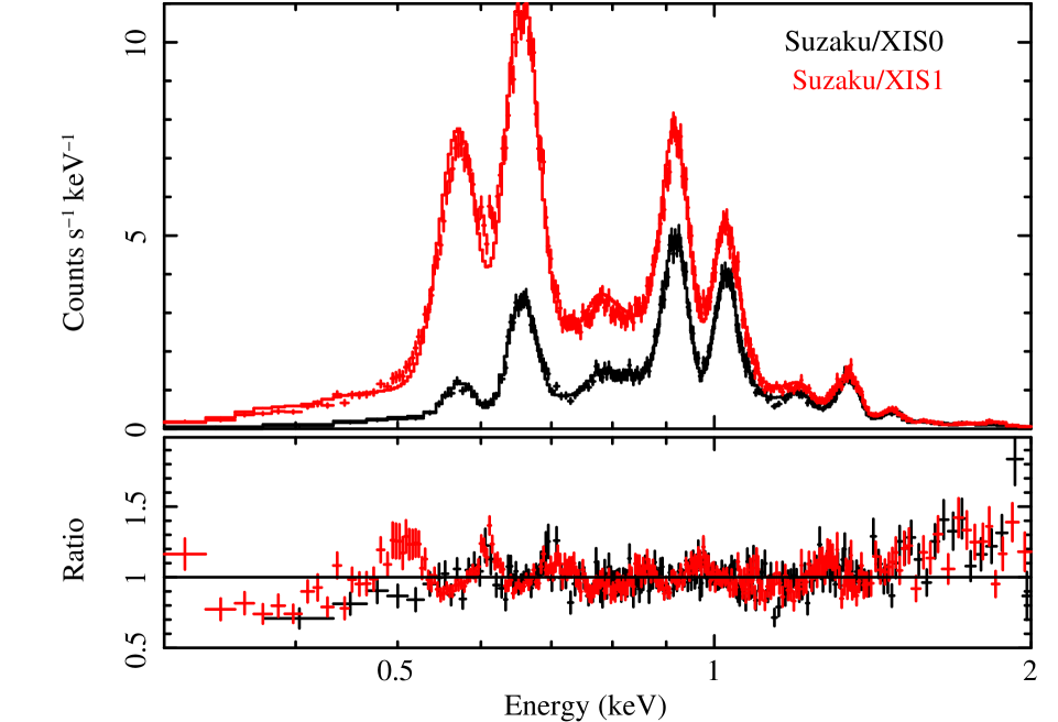
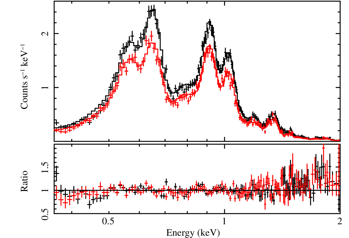
Table 9 lists the fit statistics for the various CCD instruments for the representative data sets for each instrument discussed previously. None of the fits are formally acceptable and the quality of the fit around the bright lines varies. The spectral fits with the line normalizations free are displayed in Figures 9, 10, 11, 12, and 13 for the ACIS-S3, EPIC-MOS, EPIC-pn, XIS, and XRT data respectively. The fit to the ACIS-S3 data has a reduced $\chi^{2}$ of 2.04 and appears to fit the data reasonably well with the largest residuals below 0.5 keV and above 1.5 keV. There also appears to be significantly more flux in the model around 0.8 keV than in the ACIS-S3 data. This could indicate a deficiency in the ACIS contamination model in this energy range or a problem with the weaker lines in the IACHEC model. Nevertheless, the bright O and Ne lines appear to be well-fitted and the line normalizations well-determined.

The MOS1 data have the lowest reduced $\chi^{2}$ of 1.27 and the data appear to be well-fitted with some small systematics in the residuals. The MOS2 data are almost equally well-fitted with a reduced $\chi^{2}$ of 1.30. The EPIC-MOS has the highest spectral resolution of any of the CCD instruments in this bandpass as shown by the details visible in Fig. 10. The bright lines appear to be well-fitted in the EPIC-MOS spectra. The EPIC-pn data are fitted with a reduced $\chi^{2}$ of 2.26 with large residuals on the low-energy side of the O VII triplet. The peak of the O VII triplet does not appear to be well-fitted by the IACHEC model. We suspect this is an issue with the spectral redistribution function for the EPIC-pn at these energies and the effect is under investigation. The EPIC-pn spectra do have the largest number of counts, making it somewhat easier to identify issues with the calibration. Nevertheless, the O viii Ly $\alpha$ line, the Ne ix He $\alpha$ r line, and the Ne X Ly $\alpha$ line appear to be well-fitted by the IACHEC model.

The XIS spectral fits are reasonably good ranging from a reduced $\chi^{2}$ of 1.48 for XIS0 to 1.99 for XIS1. The residuals in Fig. 12 around the O lines appear larger than the residuals around the Ne lines for both the XIS0 and XIS1. Nevertheless, the O viii Ly $\alpha$ line, the Ne ix He $\alpha$ r line, and the Ne X Ly $\alpha$ line appear to be well-fitted by the IACHEC model. The XIS spectral fit is complicated by the rapidly increasing molecular contamination. Hence the selection of this early data set when the contamination layer was still relatively small.

Figure 13 shows the 2005 Swift-XRT reference data and applied IACHEC model, obtained with the overall constant factor and line normalisations free to vary in the fit. As expected, the measured WT line normalisations (shown in Fig. 14) agree well with the model, as the WT spectrum from this epoch was used to improve the XRT QE calibration above the O-K edge at $0.545\thinspace\rm{keV}$ . Prior to the calibration change, the normalisations showed a strong energy dependence (e.g., see Fig. 3 in Plucinsky et al., 2012), indicating that the instrumental O-K edge was too shallow. The depth of this edge was subsequently increased, by thickening the silicon dioxide layer in the model of the CCD electrode structure, in order to bring the measured normalisations into better agreement with the IACHEC model. Also, the CCD spectral resolution had been slightly underestimated in the RMFs used in the earlier E0102 analysis (see the residuals in Fig. 8 in Plucinsky et al., 2012) and this was improved during the XRT response recalibration.

The PC mode line normalisations are lower that the WT ones by $5-10$ percent. We suspect the origin of this is pile-up, as an image of the PC mode data formed of diagonal events (i.e. events with grades $26-29$ ) clearly show the SNR and these events are indicative of pile-up. We have also performed a detailed simulation of the data using the XRT event simulator described by Beardmore et al. (in prep.). The simulations, which used the Chandra ACIS-S3 image to define the spatial distribution and the IACHEC model to provide the spectral distribution, confirmed that the PC mode line normalisations are suppressed by between 5 and 10 percent, whereas WT mode is unaffected.

5.3 Comparison of the Fit Results

The fitted line normalizations for the O vii He $\alpha$ r line, the O viii Ly $\alpha$ line, the Ne ix He $\alpha$ r line, & Ne X Ly $\alpha$ line are listed in Table 10. We report the normalizations for the O vii He $\alpha$ r line but the normalization of the O vii He $\alpha$ f line was the free parameter in the fit. As described in Sect. 3.2, the O vii He $\alpha$ f and r line normalizations are linked together so there is a constant factor relating the two values. The first row lists the normalization in the IACHEC model to facilitate comparison. The results for the spectral fits to the reference data for each instrument are presented in groups of three rows. Within a group of three rows for a given instrument, the first row gives the best-fitted value, the second row gives the $1.0\sigma$ lower and upper confidence limits, and the third row gives the “scaled” value where the best-fitted value has been multiplied by the constant factor. The second and third groups of rows include the results for the RGS1 and RGS2. Note that the best-fitted values and the scaled values are the same for the RGS1 since the scale factor is 1.0. This is due to the fact that the RGS data were a primary input in the development of the IACHEC model for E0102. The best-fitted values and the scaled values are different for the RGS2 since the scale factor is 0.96. The different scale factors for RGS1 and RGS2 indicate that there is a systematic 4% offset between RGS1 and RGS2 effective areas.

Table 10: Fitted Values for Constant Factor and Line Complex Normalizations

Instrument	Constant	O vii He $\alpha$ r	O viii Ly $\alpha$	Ne ix He $\alpha$ r	Ne x Ly $\alpha$
		Norm	Norm	Norm	Norm
		( $10^{-3}{\rm ph\leavevmode\nobreak\ cm^{-2}s^{-1}}$ )	( $10^{-3}{\rm ph\leavevmode\nobreak\ cm^{-2}s^{-1}}$ )	( $10^{-3}{\rm ph\leavevmode\nobreak\ cm^{-2}s^{-1}}$ )	( $10^{-3}{\rm ph\leavevmode\nobreak\ cm^{-2}s^{-1}}$ )
IACHEC
model		2.745	4.393	1.381	1.378
value
RGS1	1.0	2.700	4.404	1.400	1.415
1 $\sigma$ CL		[2.652,2.746]	[4.341,4.466]	[1.380,1.420]	[1.378,1.452]
Scaled		2.700	4.404	1.400	1.415
RGS2	0.96	no data	4.445	1.371	1.409
1 $\sigma$ CL		[—-]	[4.330,4.561]	[1.331,1.410]	[1.350,1.468]
Scaled		—-	4.267	1.316	1.353
MOS1	1.054	2.914	4.567	1.383	1.392
1 $\sigma$ CL		[2.872,2.955]	[4.514,4.620]	[1.366,1.400]	[1.373,1.411]
Scaled		3.071	4.814	1.458	1.467
MOS2	1.072	2.943	4.581	1.380	1.401
1 $\sigma$ CL		[2.899,2.987]	[4.527,4.635]	[1.363,1.397]	[1.382,1.420]
Scaled		3.155	4.911	1.479	1.502
pn	0.969	2.786	4.213	1.368	1.286
1 $\sigma$ CL		[2.778,2.794]	[4.200,4.226]	[1.364,1.372]	[1.281,1.291]
Scaled		2.700	4.082	1.326	1.246
ACIS-S3	1.072	2.230	3.803	1.311	1.375
1 $\sigma$ CL		[2.176,2.285]	[3.728,3.879]	[1.283,1.340]	[1.342,1.410]
Scaled		2.391	4.077	1.405	1.474
HETG	1.037	2.736	4.656	1.281	1.325
1 $\sigma$ CL		[2.696,2.778]	[4.604,4.707]	[1.272,1.290]	[1.313,1.337]
Scaled		2.837	4.827	1.328	1.374
XIS0	1.034	2.468	4.128	1.335	1.375
1 $\sigma$ CL		[2.385,2.556]	[4.044,4.213]	[1.311,1.358]	[1.349,1.402]
Scaled		2.552	4.268	1.380	1.422
XIS1	1.141	2.475	4.030	1.316	1.349
1 $\sigma$ CL		[2.439,2.512]	[3.981,4.080]	[1.298,1.335]	[1.328,1.371]
Scaled		2.824	4.598	1.502	1.539
XIS2	1.029	2.596	4.001	1.323	1.379
1 $\sigma$ CL		[2.512,2.679]	[3.920,4.082]	[1.300,1.347]	[1.352,1.405]
Scaled		2.671	4.117	1.361	1.419
XIS3	1.017	2.134	3.659	1.324	1.361
1 $\sigma$ CL		[2.057,2.213]	[3.581,3.738]	[1.300,1.348]	[1.334,1.388]
Scaled		2.170	3.721	1.347	1.384
XRT-PC	0.935	2.700	3.972	1.284	1.303
1 $\sigma$ CL		[2.606,2.792]	[3.859,4.087]	[1.247,1.323]	[1.260,1.346]
Scaled		2.523	3.714	1.201	1.218
XRT-WT	0.971	2.705	4.501	1.346	1.386
1 $\sigma$ CL		[2.606,2.792]	[4.390,4.615]	[1.311,1.382]	[1.346,1.427]
Scaled		2.626	4.371	1.307	1.346

Figure 14 presents the data in Table 10 in a graphical manner. The scaled normalizations for each instrument are compared to the IACHEC values and the average of all instruments is also plotted. There are several interesting trends visible in this plot. The MOS1 and MOS2 data appear to be 5-15% higher than the IACHEC model, with the O line normalizations being 10-15% higher. The EPIC-pn values have the smallest uncertainties since they are derived from a joint fit of all of the data, whereas the other instruments used a small number of observations. The EPIC-pn data agree with the IACHEC model values to better than 10% with the Ne ix He $\alpha$ r being the most discrepant at 7%. The ACIS-S3 data are most discrepant at the O lines but agree better at the Ne lines. One explanation for the O line normalizations being lower than the IACHEC values could be that there is still some residual pileup in the ACIS-S3 data suppressing the line fluxes at low energies and enhancing the line fluxes at higher energies. Another possible explanation is that the contamination model is under-predicting the absorption at the energies of the O lines at the time of these observations. As shown later in Sect. 5.4.2, the fluxes of the O lines are in better agreement with the IACHEC model for later observations. The XIS results agree to within 10% of the IACHEC model values with the exception of the O vii He $\alpha$ r line which can be discrepant by as much as 20% for XIS3. The XRT WT mode agree to within 5% of the IACHEC model whereas the XRT PC mode data can be more than 10% discrepant. As mentioned above, the XRT PC mode data most likely suffer from pileup which reduces the observed count rate.

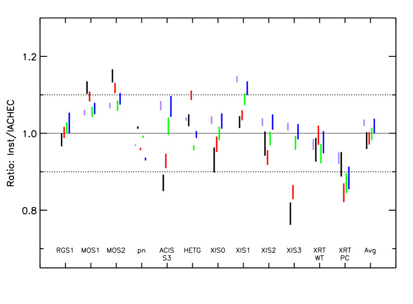
Most of the scaled normalizations agree with the IACHEC model values with $\pm 10\%$ . Specifically, 38 of the 48 normalizations are within $\pm 10\%$ of the IAHCEC model values. The scaled normalizations agree to within 10% for the Ne ix He $\alpha$ r and Ne X Ly $\alpha$ lines with the exception of the XRT PC mode data (which are affected by pileup) and the XIS1 for the Ne X Ly $\alpha$ line. The agreement is significantly worse for the O lines, $\pm 15\%$ for the O viii Ly $\alpha$ line and $\pm 25\%$ for the O vii He $\alpha$ r line. The fact that the lowest energy line produces the worst agreement is indicative of the difficulty in calibrating the spectral redistribution function and the time-dependent response of CCDs instruments at an energy as low at $\sim 570$ eV. The good agreement at higher energies for these different instruments is indicative of the quality of the calibration provided by the various instrument teams. Therefore, we conclude that the absolute effective areas of the combined systems of mirrors plus detectors agrees to within $\pm 12\%$ at 0.9 and 1.0 keV for Chandra ACIS-S3, XMM-Newton EPIC-MOS, XMM-Newton EPIC-pn, Suzaku XIS0, XIS2, & XIS3, and Swift XRT for these representative E0102 spectra.

5.4 Time Dependence of the Response

Each of the CCD instruments included in this study has a significant time dependence in its response except for the EPIC-pn. As stated in Sect. 5.1, the EPIC-pn has recorded a constant count rate from E0102 in the 0.3–2.0 keV band to better than 1.3% over the course of the mission. All of the other instruments have had a variable response for one of several reasons. Some of the instruments have developed a contamination layer that produce an additional, time-variable absorption. Some of the instruments have had significant changes in their CTI due to radiation damage that produces a time-variable spectral response. The EPIC-MOS CCDs have experienced a change in response that appears to be related to the X-ray photon does near the aimpoint of the telescope. In the following sections we discuss the time-variable response of each instrument individually.

5.4.1 XMM-Newton EPIC-MOS

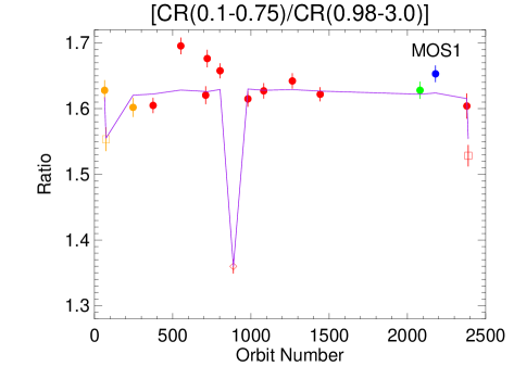
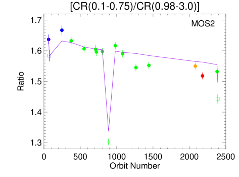
A subset of the available EPIC-MOS observations of E0102 (Table 5) was used to investigate potential trends in the effective area calibration. To minimize variance due to calibration uncertainties all observations with the same observing mode (LW mode) were selected and, with the exception of the first observation, were all positioned around 1 arcminute or so from the telescope boresight. The bulk of the observations are therefore unaffected by the redistribution patch (see Sect. 4.4). The last two observations were positioned such that the edge of the remnant just crosses the spatial area of the patch as defined within the calibration. In addition to the analysis procedure outlined in Sect. 4.4 we were careful to individually examine the spectrum from every column on the CCDs passing through the remnant. Large traps which cause sections of a given column to shift in energy by 10’s of eV are generally detected by the calibration software and a spatial correction applied to realign the reconstructed event energy to the correct scale. The frequency of these traps is increasing throughout the mission, however, and it is apparent that the current event energy calibration as used in this paper does not properly calibrate a few columns which pass through the remnant in the later observations. These columns were individually removed from the analysis and the global normalisation in the fit has been corrected for the loss of flux due to their exclusion by the same method used for bad pixels and columns excluded by the filtering process as discussed in Sect. 4.4.

The data were initially processed with SAS12.0.0 and on examining the data sample it was noticed that there was a significant trend in the spectral hardness derived from an examination of the background subtracted source count rates. In Fig. 15 we show the spectral hardness ratio defined as the source count rate in the 0.1 to 0.75 keV band divided by the rate in the 0.98 to 3.0 keV band. The actual energy boundaries used to derive this ratio has been adjusted for each observation by the gain fit parameters to ensure that the same portion of the spectrum is used in each in case. The data points have been color coded to reflect the source position relative to the boresight as the ratio is influenced by the mirror vignetting function. The ratio is also obviously dependent on the filter used in the observation. Most of the observations use the thin filter with the exception of two in medium filter (Orbit 0065 and 2380) and one observation in thick filter (Orbit 0888). Examining observations with the same filter there is a clear trend in the MOS2 data which can only plausibly be explained by the existence of a thin but growing contaminant.

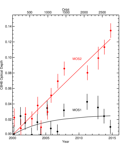
Also show on Fig. 15 is the predicted count ratio derived by folding the model E0102 spectrum through the instrument response modified by a contaminant model as described below. The model at this time consists of pure Carbon and no other compounds. The RGS detectors also suffer from a gradual loss of effective area which is presumed to be due to a carbon or carbon plus hydrogen contaminant (no edges are detected within the RGS energy passband). It is assumed the contaminant on the RGS detectors arises from outgassing of the telescope tube structure.

As EPIC shares this structure with the RGS it is plausible that the EPIC-MOS contaminant arises from the same source, however, the complicated nature of the EPIC-MOS RMF and uncertainties in its calibration make an unambiguous identification of low energy edges, even at Oxygen, very difficult. The pure Carbon model currently adopted for the EPIC-MOS is the simplest contaminant model which reasonably fits the data.

The contaminant model was derived directly from the E0102 data by finding the contaminant depth which gave the best reproduction of the observed hardness ratio (derived by folding the E0102 standard model through a response modified by the contaminant absorption) for each observation and fitting an exponential time-dependent model to the depth parameters. The models for MOS1 and MOS2 are shown in Fig. 16. Our methodology was to initially use the thin filter data only (which comprises the bulk of the observations) then compare the contamination model with observations taken with the medium and thick filters.

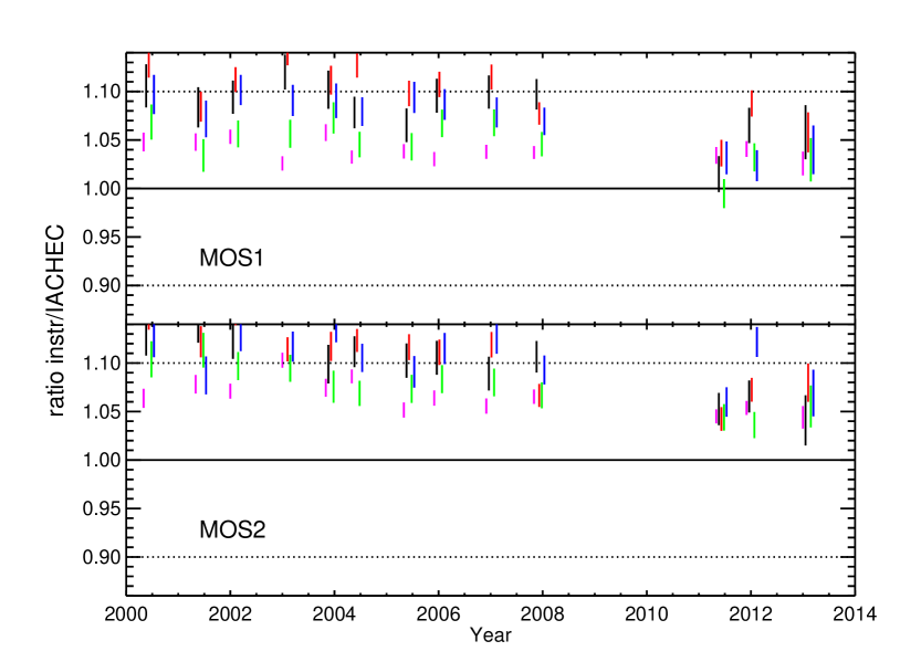
The evidence for a contaminant on MOS2 is significant but very marginal for MOS1. There is also evidence for a discontinuity in the evolution of the contamination from around orbit 1200 onwards. Further monitoring of E0102 and analysis of additional suitable calibration targets may lead to a refinement of the contamination model at a later date.

It should be noted that the predicted contaminant depth on MOS2 (around $0.04\ \mu$ m) for the latest observation in the sample was $\sim 20$ % of that on the RGS at that epoch. The contaminant is most likely on the CCD detector plane being the coldest surface (currently $-120^{\circ}$ ) on the instrument. The filter wheel assembly (at $\sim-20^{\circ}$ ) provides a warm barrier but has gaps through which molecules from the telescope tube could reach the CCDs. There is no evidence as yet for a spatial dependence of the contaminant at least within the central few arcminutes. The contaminant is not expected to be on the filters and in fact, as shown in Fig. 15 the model provides an equally good representation of the medium and thick filter ratios. In addition, dedicated calibration observations taken with the thin, medium and thick filter at the same epoch show no evidence for any change in the relative transmission of the filters since launch. The contamination model is therefore currently applied as a time-dependent adjustment to the overall EPIC-MOS detector efficiency. Finally, there is no evidence for contamination on the EPIC-pn, however, unlike the EPIC-MOS, the EPIC-pn has a cold finger trap above the detector plane. As the EPIC-MOS contaminant layer is currently relatively thin there are no immediate plans to bake-off the contaminant by heating the focal plane.

The model has been shown to improve the cross-calibration between EPIC-MOS and EPIC-pn at low energies for later epoch continuum sources and was implemented in the EPIC calibration from SAS version 13.5.0 onwards. Formally the RMF solution depends on the assumed effective area for any given standard calibration target and a new set of self-consistent RMFs were released in conjunction with the contamination model.

We have analyzed the observations listed in Table 5 with SAS version 13.5.0 and derived the five parameters from the standard IACHEC model in each case. These are shown graphically in Fig. 17 although only regular spaced observations are shown for clarity. Significant global trends in the data are now largely absent. There are some common features of the fitted parameters. Most noticeable of course is that both EPIC-MOS cameras return a higher predicted flux than the IACHEC standard model by about 10% (0.3 to 2.0 keV) although the global normalisation parameter is relatively higher in MOS2 than in MOS1 by around $\sim 3$ %. In both cameras the Ne IX He $\alpha$ r normalisation typically has the lowest relative value compared with the IACHEC model.

5.4.2 Chandra ACIS

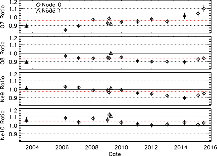
The time dependence of the low energy response of ACIS-S3 is determined primarily by the contamination layer on the filter in front of the CCDs. There are time dependent changes in the S3 CCD response to X-rays, but this is a much smaller effect than the contamination. The model for the absorption due to the ACIS contamination layer has a time dependence, a spatial dependence, and a spectral dependence. The model has been revised four times over the course of the mission, most recently in July 2014 with the release of CALDB 4.6.2. The contamination model is developed based on data from the external calibration source and celestial calibration targets other than E0102. The E0102 observations are then used to validate the contamination model as an independent check. The normalizations for the bright line complexes of the O vii He $\alpha$ r, the O viii Ly $\alpha$ line, the Ne ix He $\alpha$ r, and the Ne X Ly $\alpha$ are determined using the IACHEC model as described above. If the contamination model is accurate, the line fluxes should be constant in time within the uncertainties. In the past, clear downward trends in the E0102 line fluxes with time have prompted revisions of the contamination model.

We have determined the lines fluxes for all of the E0102 observations listed in Table 4 using the latest version of the ACIS contamination model (N0009) released in CALDB 4.6.2 on 9 July 2014 (we used CALDB 4.6.8 for this analysis but the contamination model has not changed since the CALDB 4.6.2 release). These observations are on the S3 CCD in subarray mode (to mitigate pileup), near the aimpoint which is in the middle of the CCD. The line fluxes versus time are displayed in Fig. 18 for the O vii He $\alpha$ r, the O viii Ly $\alpha$ line, the Ne ix He $\alpha$ r, and the Ne X Ly $\alpha$ line. The line fluxes for the O vii He $\alpha$ r are lower than the average from 2003-2007, are rather consistent with the average from 2007 until 2014, and then appear to be increasing after 2015. The average O vii He $\alpha$ r normalization is lower than the IACHEC value by $\sim 4\%$ . Recall that the first two observations were used for the comparison in Fig. 14 to the line normalizations for the other instruments. If later observations were used, the O vii He $\alpha$ r would be higher by $\sim 10\%$ and in better agreement with the IACHEC model. The O viii Ly $\alpha$ normalization does not show a clear trend in time. The values are mostly consistent with the average although there appears be scatter on the order of $\pm 5\%$ which is larger than statistical uncertainties. The average O viii Ly $\alpha$ normalization is lower than the IACHEC value by $\sim 7\%$ . The Ne ix He $\alpha$ r normalization shows a gradual decrease in time after 2010 but the effect is only significant at the $2\sigma$ level. The average Ne ix He $\alpha$ r normalization is lower than the IACHEC value by only $\sim 2\%$ . Finally, the Ne X Ly $\alpha$ line appears mostly constant in time within the uncertainties. The average Ne X Ly $\alpha$ normalization is higher than the IACHEC value by $\sim 5\%$ . It should be noted that there are a handful of E0102 observations towards the bottom and top of S3 that show significantly lower line normalizations than the measurements presented here in the middle of S3. The contamination layer is thicker towards the bottom and top of the S3 CCD and it appears that the current contamination model is under-predicting this gradient. This effect is under investigation and may be addressed in a future release of the contamination file.

The E0102 results on S3 indicate that the current contamination model is returning fluxes constant to within $\pm 5\%$ for the O viii Ly $\alpha$ line, the Ne ix He $\alpha$ r line, and the Ne X Ly $\alpha$ line and to within $\pm 10\%$ for the O vii He $\alpha$ r line. These results hold for observations near the middle of S3. The fluxes are constant to this level from the beginning of the Chandra mission until 2016, with the exception perhaps of the O vii He $\alpha$ r which exhibits a possible trend with time. The effective area at the energy of the O viii Ly $\alpha$ (654 eV)line has decreased by about 80% since the beginning of the mission. Therefore, the contamination model must make a large correction as a function of time for these line fluxes. E0102 will continue to be used to monitor the accuracy of the ACIS contamination model in the future.

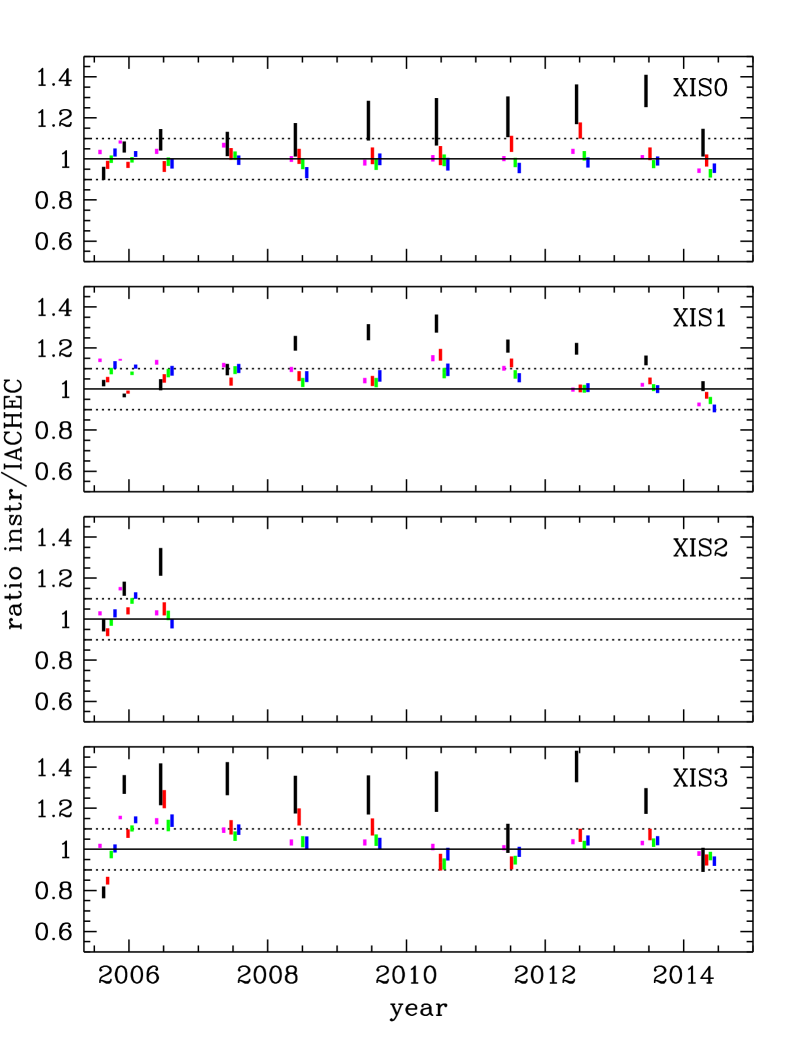
5.4.3 Suzaku XIS

The line normalizations for the Suzaku XIS depend strongly on the amount of molecular contamination, which began building up on the optical blocking filters shortly after launch. E0102 is one of three primary calibration sources for measuring the on-axis contamination build-up and chemical composition, and since the IACHEC model presented in this work is used in that analysis, there is an inherent conflict in drawing conclusive comparisons between XIS and the other instruments. Nevertheless, the quality of the contamination model can be explored here.

As can be seen in Fig. 19, except for very early in the mission, the O vii He $\alpha$ r line normalization for each XIS is 20–40% higher than the IACHEC model. The other line normalizations and overall normalization are generally within 10% of the IACHEC values, and show no strong trend except early in the mission, when the normalization increases with line energy (from O vii to Ne X). This broad-band (0.5–1 keV) energy dependence at early times possibly indicates that the column density or chemical composition of the contamination is not correct, as the increasing line normalization with energy mimics the effects of an underestimated oxygen absorption edge. At later times, only O VII is discrepant, which could result from an incorrectly modeled low-energy redistribution tail becoming apparent as the X-ray sensitivity decreases.

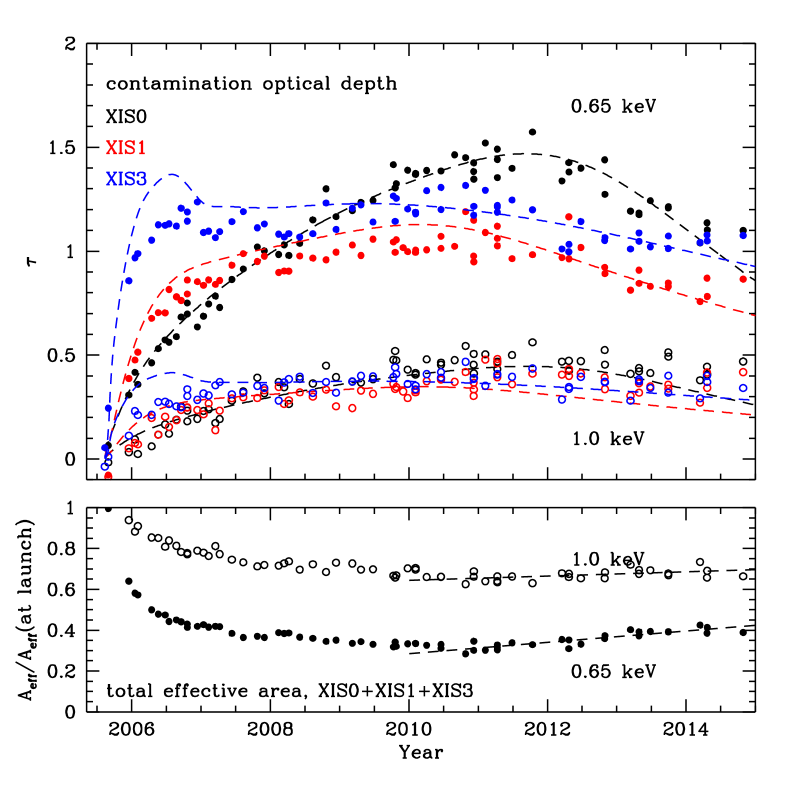
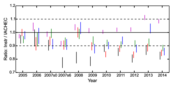
The quality of the calibration can be seen by comparing Fig. 19 with Fig. 20, which shows the optical depth and fractional effective area at two energies, 0.65 keV and 1.0 keV. These estimates are made by fitting simple Gaussians to the bright O VIII Ly $\alpha$ and Ne X Ly $\alpha$ lines, along with a simple model for the continuum and other lines, and comparing those line normalizations to the IACHEC values. The dashed lines in the top panel show the current contamination CALDB for an on-axis source, produced from multiple calibration sources including E0102. Several things are apparent from this figure. First, the contamination built up very quickly, reaching nearly a maximum on XIS3 within 6 months. This is about the level that ACIS reached after several years. Modeling the build-up early is hampered by a lack of calibration observations during this time. Second, the measured line normalizations for XIS3 (and to a lesser extent XIS1) do not match the CALDB well between 2005 and 2008, with a bump-like feature in the CALDB trend that is not reflected in the data points. These calibration issues will be addressed in future work.

5.4.4 Swift XRT

Figure 21 show the temporal behavior of the line normalisations for the Swift-XRT WT data, with representative spectra (from 2009, 2011, 2013) shown in Fig. 22. The latter, when compared with Fig. 13, illustrates how the spectral resolution has degraded with time, even with CCD charge trap corrections applied. The line normalisations are initially well behaved, but from the second half of 2007 show an occasional loss in line flux, particularly in the lowest energy line (i.e. the O vii He $\alpha$ near $0.57\thinspace\rm{keV}$ ) in 2007(s6), 2008 and 2009.

This discrepant behavior appears to occur when the main emitting ring of the remnant (radius $10-18\arcsec$ ) falls on the CCD bad-column gaps. Gaetz et al. (2000) and Flanagan et al. (2004) show that the line components have different spatial origins, with O vii He $\alpha$ r arising predominantly from the south-east quadrant of the ring, while Ne x Ly $\alpha$ r is more symmetrically formed in the ring. Individual snapshots are quite frequently placed with parts of the remnant on the CCD bad columns. Depending on the orientation of the remnant with respect to the bad-columns we can see a suppression of all four line fluxes compared to the IACHEC model, or sometimes a more preferentially loss of the O vii He $\alpha$ component. At this point in time, it is not possible to account for these effects as no method exists to correct for such spatial-spectral variation when the ARFs are generated.

Other factors could contribute to the normalisation variations, such as the existence of deep charge traps which remove events below the onboard threshold, or a response kernel width which does not quite match the data. While other missions report time variable low energy contamination, we do not think that such a problem exists for the Swift-XRT, because observations of low column density sources show no significant increases in the inferred column density with time.

6 Discussion

6.1 Comparison with Other Cross-Calibration Studies

6.1.1 XMM-Newton Internal Cross-calibration Studies

There have been several studies of the cross-calibration amongst the instruments on XMM-Newton. Mateos et al. (2009) used 2XMM sources that were bright enough to have sufficient counts but not bright enough to have significant pileup to compare the derived fluxes in several energy bands: 0.2–0.5, 0.5–1.0, 1.0–2.0, 2.0–4.5, and 4.5–12.0 kev. The data were processed with SAS v7.1 and the calibration files available at that time. Of interest for our study, Mateos et al. (2009) found that on-axis sources returned a MOS1/MOS2 flux that was 5-7 % higher than the EPIC-pn flux in the 0.5–1.0 keV band. Stuhlinger et al. (2010) conducted a similar analysis after processing the data with SAS v10.0 and compared the EPIC-MOS and EPIC-pn fluxes in several narrow bands using 2XMM sources that were not piled-up. In their 0.54–0.85 keV band, they found that the MOS1 and EPIC-pn returned nearly identical fluxes, while the MOS2 returned fluxes that were on average 5% higher than EPIC-pn fluxes. An update of this analysis with SAS v15.0 shows MOS1/MOS2 returning 4/7% higher fluxes in the 0.54–0.85 keV band than EPIC-pn; however, the distribution of values spans the range from 0–12%.

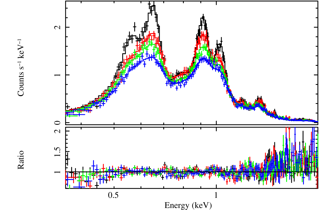
Read et al. (2014) conducted a similar analysis with on-axis 2XMM sources after processing the data with SAS v12.0. They used the “stacked residuals” method to quantify the derived flux differences between EPIC-MOS and EPIC-pn on a finer energy scale. They find that the flux difference between MOS1/MOS2 and EPIC-pn peaks at around 5% at an energy of $\sim 0.6$ keV in the 0.5–1.0 keV band (with the MOSs returning higher fluxes), while at other energies in the 0.5–1.0 keV band the difference is typically a few percent. For the E0102 line fluxes described in this paper, EPIC-MOS and EPIC-pn differ by 10-15% in the 0.5–1.0 keV bandpass. It should be noted that the RGS effective area below 0.5 keV was adjusted to agree better with the EPIC-pn in SAS v10.0. It is not clear why the results are apparently significantly different for 2XMM sources on-axis compared to E0102 on-axis. E0102 is obviously an extended source but given that the diameter is only 45″, it is difficult to understand how the effective area could be that different at such small off-axis angles compared to on-axis. The flux in the E0102 spectrum is mostly concentrated in the four bright line complexes that we have fit in this paper, while the 2XMM sources have spectra that more closely resemble a continuum in the 0.5–1.0 keV band. There are several effects contributing at the $\sim 1\%$ level, that might contribute to this discrepancy. For example, there is still pileup in the EPIC-MOS and EPIC-pn, the use of a point source PSF is an approximation, the vignetting function is also approximated, the gain fit effects the line normalizations, and the point source analysis still does not include 100% of the encircled energy fraction. This apparent discrepancy remains under investigation.

6.1.2 External Cross-calibration Studies

There have been several analyses initiated by the IACHEC to compare the cross-calibration of the effective areas of the current generation of X-ray instruments. Tsujimoto et al. (2011) used the Galactic SNR G21.5-0.9 to compare the effective area in the 2.0–8.0 keV range for Chandra, XMM-Newton, Swift, and Suzaku using the calibration products available at the writing of that paper. G21.5-0.9 has a highly absorbed spectrum with an $N_{\mathrm{H}}$ of $\sim 3.0\times 10^{22}\leavevmode\nobreak\ {\rm cm^{-2}}$ such that there is little flux below 2.0 keV. Tsujimoto et al. (2011) found that the 2.0–8.0 keV fluxes generally agreed to within $\pm 10\%$ , with the maximum discrepancy being between ACIS-S3 and EPIC-pn with ACIS-S3 producing a flux $\sim 16\%$ higher than EPIC-pn. Ishida et al. (2011) used the BL Lac object PKS 2155-304 to compare the derived spectral parameters (power-law index and column density) for XIS, EPIC-MOS, EPIC-pn, and the Low-Energy Transmission Grating (LETG) on Chandra used with both ACIS and the High Resolution Camera (HRC). Since E0102 has not been observed with the LETG on Chandra, we can not compare the results of Ishida et al. (2011) to our results. Although the primary objective of this study was to compare the consistency of the fitted parameters that determine the shape of the spectrum, Ishida et al. (2011) did compute fluxes in narrow bands. Since PKS 2155-304 is variable, both in intensity and spectral shape, the observations had to be executed simultaneously or as simultaneous as possible given the scheduling constraints of the observatories. They computed the fluxes in several bands from 0.5 to 10.0 keV, the most relevant for comparison to our results is the 0.5–1.0 keV band. There were three simultaneous observations with XMM-Newton and Suzaku in 2005, 2006, and 2008. The EPIC-pn, EPIC-MOS, and XIS fluxes agree to within 10% in the 0.5–1.0 keV band, although the order of which instrument produces the highest flux is not the same for the three epochs. The EPIC-pn produces higher fluxes than the MOS1 in all three epochs, in disagreement with the studies based on 2XMM sources. The XIS1 produces the lowest average flux, while the XIS0 is higher than the XIS1. The order of which instrument produces the higher flux is opposite to what we observe with E0102. They observe the EPIC-pn to produce higher fluxes than the EPIC-MOS and XIS0 to produce higher fluxes than XIS1. The differences are on the order of 5% so this may be an indication of the systematic uncertainties that persist in our analyses. Or it might be indicating something fundamentally different in the calibration of extended sources with line-dominated spectra compared to point sources with continua spectra.

There have a been a series of papers motivated by the IACHEC using cluster of galaxies to compare the calibration of the current generation of instruments. Nevalainen et al. (2010) used a sample of relaxed clusters to compare the temperatures and fluxes derived by XMM-Newton, Chandra, and BeppoSAX. Nevalainen et al. (2010) computed fluxes in a hard band (2.0–7.0 keV) and a soft band (0.5-2.0 keV). They found that the ACIS fluxes were on average 11% higher than the EPIC-pn fluxes in the hard band, similar to the findings of Tsujimoto et al. (2011) in a similar band. In the soft band, they find that the ACIS and EPIC-pn fluxes agree on average to within 2%, however the scatter is large with outliers at -10% and +14%. It is not clear what the explanation is for the relatively large scatter in this cluster sample. Kettula et al. (2013) expanded this study to include the XISs on Suzaku. They noted discrepancies between the XIS0, XIS1, and XIS3 in the derived spectral shape that could be addressed with a modification to the Suzaku contamination model. Later releases of the contamination model brought the three XISs into better agreement. Schellenberger et al. (2015) analyzed 63 clusters from the HIFLUGCS sample (Reiprich & Böhringer, 2002) performing a similar analysis as Nevalainen et al. (2010) using the most recent software and calibration at the time of writing that paper, CIAO 4.5 and CALDB 4.5.5.1 for Chandra and SAS v12.0.1 and CCF dated 14.12.2012 for XMM-Newton. Schellenberger et al. (2015)’s primary objective was to characterize any systematic difference in the derived temperatures of clusters for cosmology, but they did conduct a stacked residuals analysis similar to Read et al. (2014) to characterize differences in the effective area calibration. They find in the 0.5–1.0 keV band that ACIS produces 0–10% higher fluxes than EPIC-pn and MOS1/MOS1 produce 0–5% higher fluxes in rough agreement with Read et al. (2014).

The studies described above used sources with different properties (point vs. extended, thermal vs. non-thermal spectra, etc.) and used different versions of the calibration files and analysis software. Therefore, it is difficult to know if the results would be more consistent if the same calibration files and analysis software were used on the same types of sources. Nevertheless, the majority of the studies indicate that ACIS produces the highest fluxes in the 0.5–1.0 keV band, the EPIC-MOS produces the second highest fluxes, and the EPIC-pn produces the lowest fluxes.

6.2 The E0102 Cross-calibration Results

The cross-calibration results using E0102 presented in Table 10 and Fig. 14 differ from the previous studies in several ways. It is clearest to discuss the differences line by line or equivalently, energy by energy. At the energy of the O vii He $\alpha$ r ( $\sim 570\leavevmode\nobreak\ eV$ ), MOS1/MOS2 produce significantly higher fluxes than EPIC-pn, and ACIS-S3 produces the lowest fluxes. All XISs produce fluxes consistent with the IACHEC model value except for XIS3 which is $\sim 20\%$ lower than the IACHEC value. The XRT WT mode data are within 5% of the IACHEC value (for the remainder of this discussion we will limit the discussion to the XRT WT mode data since they agree better with the IACHEC model than the PC mode data). The relative ordering of ACIS-S3, EPIC-pn, and MOS1/MOS2 is different than what the stacked residuals method with clusters and 2XMM sources determined. It should be noted that the E0102 analysis is sampling the response of the instruments in a narrower range of energies (essentially a line) for the CCD instruments while the stacked residuals approach must necessarily sum over a range of pulse-heights or energies. The agreement at the energy of O viii Ly $\alpha$ line ( $\sim 654\leavevmode\nobreak\ eV$ ) is better in terms of the magnitude of the difference. The XIS instruments agree better with the IACHEC model value except for XIS3 which is $\sim 15\%$ lower than the IACHEC value. The ACIS-S3 value is in agreement with the EPIC-pn value and both are only slightly lower than the IACHEC value and the XRT WT mode data are in excellent agreement with the IACHEC value. The EPIC-MOS values are $\sim 15\%$ higher than the EPIC-pn value. But the relative order of ACIS-S3, EPIC-pn, and EPIC-MOS are different again compared to the stacked residuals approach. At the energy of the Ne ix He $\alpha$ r ( $\sim 922\leavevmode\nobreak\ eV$ ), the agreement is within 10% for all instruments. At the energy of the Ne X Ly $\alpha$ line ( $\sim 1022\leavevmode\nobreak\ eV$ ), the agreement is within 15% for all instruments. It is somewhat surprising that the MOS1/MOS2 and EPIC-pn disagree by 10-15% at this energy.

The fact that ACIS-S3 and XIS disagree with the IACHEC model the most at the lowest energy line for which we conducted a comparison could indicate a deficiency in the contamination models for each instrument. ACIS-S3 and the XIS have the largest correction for a contamination layer of any of the instruments. As noted earlier, if later ACIS-S3 observations were used for this comparison, the O vii He $\alpha$ r normalization would be larger than it was for the first two ACIS-S3 observations used and in better agreement with the IACHEC model. This might also indicate that there is some residual pileup which is depressing the fluxes of the lowest energy lines in the ACIS-S3 data. The latest XIS observations indicated that the contamination layer on Suzaku was getting thinner with time. Both of these facts indicate how challenging it is to develop an accurate contamination model for all times of a mission.

E0102 is fundamentally different from the point sources and clusters used in the stacked residuals analyses. First, E0102 has a line-dominated spectrum where the majority of the flux in the 0.5–1.0 keV band is produced by 4 lines/line complexes. The response of these instruments is changing rapidly over the 0.5–1.0 keV band. Therefore, it is possible that the E0102 data might reveal issues with the calibration as a function of energy more clearly than a continuum source. Second, E0102 is an extended source with a diameter of 45″. The point sources from the 2XMM analyses sample a different part of the detectors and the point-spread function of the telescope, although one hopes that the telescope response changes little over 45″. There may still be some residual pileup affecting the 2XMM sources. The cluster analysis samples a much larger region on the detector and larger off-axis angles than the E0102 analysis. For these reasons, each of these studies is probing different aspects of the instruments’ calibrations.

The time-dependent line normalizations we presented highlight the challenges in providing an accurate calibration throughout a mission as the CCD response changes due to radiation damage and the accumulation of a contamination layer. The EPIC-pn instrument has the most stable response and in this respect has the simplest job in providing a time-dependent calibration. Both ACIS-S3 and the XIS have a time-variable contamination layer that has a complex time dependence. For the XIS, the contamination layer grew at different rates on the different detectors and appeared to be decreasing at the end of the mission. For ACIS, the accumulation rate has varied over the mission and the chemical composition has also changed with time. Given how much the ACIS-S3 and XIS response have changed in the 0.5–1.0 keV over the mission, it is encouraging that the line normalizations are as stable as they are with time. The EPIC-MOS response has changed because of the “patch” effect in the CCDs and the accumulation of a contamination layer. Fortunately for the EPIC-MOS, the contamination layer is much thinner than on ACIS or the XIS and it has been simpler to model. The XRT WT mode data have exhibited significant evolution with time, with the lowest energy line normalizations decreasing the most with time. This behavior might be explained by the placement of E0102 on bad columns that are increasing with time. The E0102 analysis presented here is the first of these cross-calibration studies to characterize the time-dependent response of these instruments. It is our hope that the Guest Observer community for these missions can use these results to assess the reliability of their results.

7 Conclusions

We have used the line-dominated spectrum of the SNR E0102 to test the response models of the ACIS-S3, EPIC-MOS, EPIC-pn, XIS, and XRT CCDs below 1.5 keV. We have fitted the spectra with the same model in which the continuum and absorption components and the weak lines are held fixed while allowing only the normalizations of four bright lines/line complexes to vary. We have compared the fitted line normalizations of the O vii He $\alpha$ r line, the O viii Ly $\alpha$ line, the Ne ix He $\alpha$ r line, and Ne X Ly $\alpha$ line to examine the consistency of the effective area models for the various instruments in the energy ranges around 570 eV, 654 eV, 915 eV, and 1022 eV. We find that the instruments are in general agreement with 38 of the 48 scaled normalizations within $\pm 10\%$ of the IACHEC model values. However, the agreement is better for the higher energy lines than the low energy lines. We find that the scaled line normalizations agree with the IACHEC model normalization to within $\pm 9\%$ & $\pm 12\%$ for the Ne ix He $\alpha$ r & Ne X Ly $\alpha$ line complexes when all instruments are considered (if we adopt the Swift XRT WT mode results and exclude the PC mode results). The agreement is significantly worse for the low energy lines, as the scaled line normalizations agree with the IACHEC model normalization to within $\pm 20\%$ & $\pm 15\%$ for the O vii He $\alpha$ r and O viii Ly $\alpha$ r line complexes. This difference with energy emphasizes the challenges presented by the low energy calibration of these CCD instruments. When only Chandra and XMM-Newton are considered, we find that the fitted line normalizations agree with the IACHEC normalization to within $\pm 15\%$ , $\pm 12\%$ , $\pm 8\%$ , & $\pm 9\%$ for O vii He $\alpha$ r, O viii Ly $\alpha$ , Ne ix He $\alpha$ r, & Ne X Ly $\alpha$ . Therefore, the absolute effective areas of Chandra ACIS-S3, XMM-Newton EPIC-pn, and XMM-Newton-MOS agree to better than $\pm 10\%$ at 0.9 and 1.0 keV for the time intervals and data modes considered in this analysis.

The time dependence of each of the CCD instruments was presented. All of the CCD instruments have a significant variation in response with time except for the XMM-Newton EPIC-pn which measures a flux in the 0.3–2.0 keV band consistent to 1.3% over the course of the mission. The derived normalizations with time for ACIS-S3, EPIC-MOS, XIS, and XRT for the O vii He $\alpha$ r line, the O viii Ly $\alpha$ line, the Ne ix He $\alpha$ r line, and Ne X Ly $\alpha$ line can be used to assess the reliability of the effective area calibration at a given point in time for the respective mission/instrument.

Acknowledgements.

This work was supported by NASA contract NAS8-03060. APB acknowledges support from the UK Space Agency. We thank Daniel Dewey for the analysis of the HETG data that was critical in the development of the IACHEC standard model for E0102. We thank Joseph DePasquale and Jennifer Posson-Brown for their years of assistance in analyzing the Chandra data of E0102 that developed the methods and software for the ACIS analysis. We thank Randall Smith for helpful discussions about the use of the APEC models. We thank Herman Marshall and Alexey Vikhlinin for helpful discussions on the analysis and the modifications to the ACIS contamination model. We thank Marcus Kirsch who took a leadership role in setting up the IACHEC and Matteo Guainazzi for leading the IACHEC over the last several years.

References

Arnaud et al. (1999) Arnaud, K., Dorman, B., & Gordon, C. 1999, Astrophysics Source Code Library, 10005
Bautz et al. (1998) Bautz, M., Pivovaroff, M., Baganoff, F., et al. 1998, in X-Ray Optics, Instruments, and Missions, ed. R. B. Hoover & A. B. W. II, Vol. 3444, 210
Behar et al. (2001) Behar, E., Rasmussen, A. P., Griffiths, R. G., et al. 2001, A&A, 365, L242
Blair et al. (2000) Blair, W. P., Morse, J. A., Raymond, J. C., et al. 2000, ApJ, 537, 667
Blair et al. (1989) Blair, W. P., Raymond, J. C., Danziger, J., & Matteucci, F. 1989, ApJ, 338, 812
Borkowski et al. (2007) Borkowski, K. J., Hendrick, S. P., & Reynolds, S. P. 2007, ApJ, 671, L45
Burrows et al. (2005) Burrows, D. N., Hill, J. E., Nousek, J. A., et al. 2005, Space Science Reviews, 120, 165
Canizares et al. (2005) Canizares, C. R., Davis, J. E., Dewey, D., et al. 2005, PASP, 117, 1144
Canizares et al. (2000) Canizares, C. R., Huenemoerder, D. P., Davis, D. S., et al. 2000, ApJ, 539, L41
Cash (1979) Cash, W. 1979, ApJ, 228, 939
de Vries et al. (2015) de Vries, C. P., den Herder, J. W., Gabriel, C., et al. 2015, A&A, 573, A128
den Herder et al. (2001) den Herder, J. W., Brinkman, A. C., Kahn, S. M., et al. 2001, A&A,, 365, L7
DePasquale et al. (2004) DePasquale, J. M., Plucinsky, P. P., Vikhlinin, A. A., et al. 2004, in Optical and Infrared Detectors for Astronomy. Edited by Garnett, James D.; Beletic, James W. Proceedings of the SPIE, Volume 5501, pp. 328-338 (2004)., ed. A. D. Holland, 328–338
Dewey (2002) Dewey, D. 2002, in High Resolution X-ray Spectroscopy with XMM-Newton and Chandra, ed. G. Branduardi-Raymont
Dewey & Noble (2009) Dewey, D. & Noble, M. S. 2009, in Astronomical Data Analysis Software and Systems XVIII, ed. D. A. Bohlender, D. Durand, & P. Dowler, Vol. 411, 234
Dopita et al. (1981) Dopita, M. A., Tuohy, I. R., & Mathewson, D. S. 1981, ApJ, 248, L105
Evans et al. (2009) Evans, P. A., Beardmore, A. P., Page, K. L., et al. 2009, MNRAS, 397, 1177
Finkelstein et al. (2006) Finkelstein, S. L., Morse, J. A., Green, J. C., et al. 2006, ApJ, 641, 919
Flanagan et al. (2004) Flanagan, K. A., Canizares, C. R., Dewey, D., et al. 2004, ApJ, 605, 230
Foster et al. (2012) Foster, A. R., Ji, L., Smith, R. K., & Brickhouse, N. S. 2012, ApJ, 756, 128
Gaetz et al. (2000) Gaetz, T. J., Butt, Y. M., Edgar, R. J., et al. 2000, ApJL,, 534, L47
Garmire et al. (1992) Garmire, G., Ricker, G., Bautz, M., et al. 1992, in American Institute of Aeronautics and Astronautics Conference, 8
Garmire et al. (2003) Garmire, G. P., Bautz, M. W., Ford, P. G., Nousek, J. A., & Ricker, G. R. 2003, in X-Ray and Gamma-Ray Telescopes and Instruments for Astronomy, ed. J. Truemper & H. Tananbaum, Vol. 4851, 28–44
Gehrels et al. (2004) Gehrels, N., Chincarini, G., Giommi, P., et al. 2004, ApJ, 611, 1005
Godet et al. (2009) Godet, O., Beardmore, A. P., Abbey, A. F., et al. 2009, A&A, 494, 775
Godet et al. (2007) Godet, O., Beardmore, A. P., Abbey, A. F., et al. 2007, in Presented at the Society of Photo-Optical Instrumentation Engineers (SPIE) Conference, Vol. 6686, UV, X-Ray, and Gamma-Ray Space Instrumentation for Astronomy XV. Edited by Siegmund, Oswald H. Proceedings of the SPIE, Volume 6686, pp. 66860A-66860A-8 (2007).
Hill et al. (2004) Hill, J. E., Burrows, D. N., Nousek, J. A., et al. 2004, in Proc. SPIE, Vol. 5165, X-Ray and Gamma-Ray Instrumentation for Astronomy XIII, ed. K. A. Flanagan & O. H. W. Siegmund, 217–231
Houck (2002) Houck, J. C. 2002, in High Resolution X-ray Spectroscopy with XMM-Newton and Chandra, Proceedings of the international workshop held at the Mullard Space Science Laboratory of University College London, Holmbury St Mary, Dorking, Surrey, UK, October 24 - 25, 2002, Ed. Branduardi-Raymont, G., published electronically and stored on CD., meeting abstract, ed. G. Branduardi-Raymont
Huenemoerder et al. (2011) Huenemoerder, D. P., Mitschang, A., Dewey, D., et al. 2011, AJ, 141, 129
Hughes et al. (2000) Hughes, J. P., Rakowski, C. E., & Decourchelle, A. 2000, ApJL, 543, L61
Humphrey et al. (2009) Humphrey, P. J., Liu, W., & Buote, D. A. 2009, ApJ, 693, 822
Ishida et al. (2011) Ishida, M., Tsujimoto, M., Kohmura, T., et al. 2011, PASJ, 63, S657
Jansen et al. (2001) Jansen, F., Lumb, D., Altieri, B., et al. 2001, A&A,, 365, L1
Kettula et al. (2013) Kettula, K., Nevalainen, J., & Miller, E. D. 2013, A&A, 552, A47
Koyama et al. (2007) Koyama, K., Tsunemi, H., Dotani, T., et al. 2007, PASJ, 59, 23
Marshall et al. (2004) Marshall, H. L., Tennant, A., Grant, C. E., et al. 2004, in X-Ray and Gamma-Ray Instrumentation for Astronomy XIII. Edited by Flanagan, Kathryn A.; Siegmund, Oswald H. W. Proceedings of the SPIE, Volume 5165, pp. 497-508 (2004)., ed. K. A. Flanagan & O. H. W. Siegmund, 497–508
Mateos et al. (2009) Mateos, S., Saxton, R. D., Read, A. M., & Sembay, S. 2009, A&A, 496, 879
Nevalainen et al. (2010) Nevalainen, J., David, L., & Guainazzi, M. 2010, A&A, 523, A22
Nousek & Shue (1989) Nousek, J. A. & Shue, D. R. 1989, ApJ, 342, 1207
Ozawa et al. (2009) Ozawa, M., Uchiyama, H., Matsumoto, H., et al. 2009, PASJ, 61, 1
Pagani et al. (2011) Pagani, C., Beardmore, A. P., Abbey, A. F., et al. 2011, A&A, 534, A20
Patnaude & Fesen (2007) Patnaude, D. J. & Fesen, R. A. 2007, AJ, 133, 147
Patnaude & Fesen (2009) Patnaude, D. J. & Fesen, R. A. 2009, ApJ, 697, 535
Patnaude et al. (2011) Patnaude, D. J., Vink, J., Laming, J. M., & Fesen, R. A. 2011, ApJ, 729, L28
Plucinsky et al. (2012) Plucinsky, P. P., Beardmore, A. P., DePasquale, J. M., et al. 2012, in Society of Photo-Optical Instrumentation Engineers (SPIE) Conference Series, Vol. 8443, Society of Photo-Optical Instrumentation Engineers (SPIE) Conference Series
Plucinsky et al. (2008) Plucinsky, P. P., Haberl, F., Dewey, D., et al. 2008, in Society of Photo-Optical Instrumentation Engineers (SPIE) Conference Series, Vol. 7011, Society of Photo-Optical Instrumentation Engineers (SPIE) Conference Series
Plucinsky et al. (2003) Plucinsky, P. P., Schulz, N. S., Marshall, H. L., et al. 2003, in X-Ray and Gamma-Ray Telescopes and Instruments for Astronomy. Edited by Joachim E. Truemper, Harvey D. Tananbaum. Proceedings of the SPIE, Volume 4851, pp. 89-100 (2003)., ed. J. E. Truemper & H. D. Tananbaum, 89–100
Rasmussen et al. (2001) Rasmussen, A. P., Behar, E., Kahn, S. M., den Herder, J. W., & van der Heyden, K. 2001, A&A,, 365, L231
Read et al. (2014) Read, A. M., Guainazzi, M., & Sembay, S. 2014, A&A, 564, A75
Reiprich & Böhringer (2002) Reiprich, T. H. & Böhringer, H. 2002, ApJ, 567, 716
Rho et al. (2009) Rho, J., Reach, W. T., Tappe, A., et al. 2009, ApJ, 700, 579
Russell & Bessell (1989) Russell, S. C. & Bessell, M. S. 1989, ApJS, 70, 865
Russell & Dopita (1990) Russell, S. C. & Dopita, M. A. 1990, ApJS, 74, 93
Russell & Dopita (1992) Russell, S. C. & Dopita, M. A. 1992, ApJ, 384, 508
Sartore et al. (2012) Sartore, N., Tiengo, A., Mereghetti, S., et al. 2012, A&A, 541, A66
Sasaki et al. (2006) Sasaki, M., Gaetz, T. J., Blair, W. P., et al. 2006, ApJ, 642, 260
Sasaki et al. (2001) Sasaki, M., Stadlbauer, T. F. X., Haberl, F., Filipović, M. D., & Bennie, P. J. 2001, A&A, 365, L237
Schellenberger et al. (2015) Schellenberger, G., Reiprich, T. H., Lovisari, L., Nevalainen, J., & David, L. 2015, A&A, 575, A30
Sembay et al. (2011) Sembay, S., Saxton, R., & Guainazzi, M. 2011, in The X-ray Universe 2011, ed. J.-U. Ness & M. Ehle, 283
Seward & Mitchell (1981) Seward, F. D. & Mitchell, M. 1981, ApJ,, 243, 736
Smith et al. (2001) Smith, R. K., Brickhouse, N. S., Liedahl, D. A., & Raymond, J. C. 2001, ApJL, 556, L91
Strüder et al. (2001) Strüder, L., Briel, U., Dennerl, K., et al. 2001, A&A,, 365, L18
Stuhlinger et al. (2010) Stuhlinger, M., Smith, M. J. S., Guainazzi, M., et al. 2010, http://xmm.vilspa.esa.es/docs/documents/CAL-TN-0052.ps.gz
Tsujimoto et al. (2011) Tsujimoto, M., Guainazzi, M., Plucinsky, P. P., et al. 2011, A&A, 525, A25
Tuohy & Dopita (1983) Tuohy, I. R. & Dopita, M. A. 1983, ApJ, 268, L11
Turner et al. (2001) Turner, M. J. L., Abbey, A., Arnaud, M., et al. 2001, A&A,, 365, L27
Vogt & Dopita (2010) Vogt, F. & Dopita, M. A. 2010, ApJ, 721, 597
Weisskopf et al. (2002) Weisskopf, M. C., Brinkman, B., Canizares, C., et al. 2002, Publications of the Astronomical Society of the Pacific, 114, 1
Weisskopf et al. (2000) Weisskopf, M. C., Tananbaum, H. D., Van Speybroeck, L. P., & O’Dell, S. L. 2000, in X-Ray Optics, Instruments, and Missions III, ed. J. E. Truemper & B. Aschenbach, Vol. 4012, 2
Wilms et al. (2000) Wilms, J., Allen, A., & McCray, R. 2000, ApJ, 542, 914