Impacts of fragmented accretion streams onto Classical T Tauri Stars: UV and X-ray emission lines

Abstract

Context. The accretion process in Classical T Tauri Stars (CTTSs) can be studied through the analysis of some UV and X-ray emission lines which trace hot gas flows and act as diagnostics of the post-shock downfalling plasma. In the UV band, where higher spectral resolution is available, these lines are characterized by rather complex profiles whose origin is still not clear.

Aims. We investigate the origin of UV and X-ray emission at impact regions of density structured (fragmented) accretion streams. We study if and how the stream fragmentation and the resulting structure of the post-shock region determine the observed profiles of UV and X-ray emission lines.

Methods. We model the impact of an accretion stream consisting of a series of dense blobs onto the chromosphere of a CTTS through 2D MHD simulations. We explore different levels of stream fragmentation and accretion rates. From the model results, we synthesize C IV (1550 Å) and O VIII (18.97 Å) line profiles.

Results. The impacts of accreting blobs onto the stellar chromosphere produce reverse shocks propagating through the blobs and shocked upflows. These upflows, in turn, hit and shock the subsequent downfalling fragments. As a result, several plasma components differing for the downfalling velocity, density, and temperature are present altoghether. The profiles of C IV doublet are characterized by two main components: one narrow and redshifted to speed $\approx 50$ km s^-1 and the other broader and consisting of subcomponents with redshift to speed in the range $200-400$ km s^-1. The profiles of O VIII lines appear more symmetric than C IV and are redshifted to speed $\approx 150$ km s^-1.

Conclusions. Our model predicts profiles of C IV line remarkably similar to those observed and explains their origin in a natural way as due to stream fragmentation.

1 Introduction

Classical T Tauri Stars (CTTS) are young stars surrounded by an accretion disk. According to the magnetospheric accretion scenario, gas from the disk accretes onto the star through accretion columns (Koenigl, 1991). Several lines of evidence support this picture especially in the optical and infrared bands (e.g. Bertout et al. 1988). Also accreting T Tauri Stars show a soft X-ray (0.2-0.8 KeV) excess, with typical lines produced at temperatures $10^{5}-10^{6}$ K. This excess has been interpreted as due to impacts of the accreting material with the stellar surface where a shock is produced and dissipates the kinetic energy of the downfalling material (Koenigl, 1991). The shock heats the plasma up to temperatures of few million degrees, causing X-ray emission (Kastner et al., 2002; Argiroffi et al., 2007). The heated plasma is characterized by density of $n\approx 10^{11}-10^{13}$ cm^-3 (e.g. Argiroffi et al. 2007).

The interpretation of the soft X-ray excess in CTTSs in terms of accretion shocks is well supported by hydrodynamic (HD) and magnetohydrodynamic (MHD) models. Time-dependent 1D model of radiative accretion shocks in CTTSs provided a first accurate description of the dynamics of the postshock plasma (Koldoba et al., 2008; Sacco et al., 2008). In particular Sacco et al. (2008) proposed a one.dimensional hydrodynamic (HD) model of a continuous accretion flow impacting onto the chromosphere of a CTTS, thus assuming the ratio between the thermal pressure and the magnetic pressure $\beta<<1$. Their model reproduced the main features of high spectral resolution X-ray observations of the CTTS MP Mus that was previously interpreted as due to postshock plasma (Argiroffi et al., 2007)

More recently 2D MHD models of accretion impacts have been studied (Orlando et al. 2010; Matsakos et al. 2013; Orlando et al. 2013) to explore those cases where the low-$\beta$ approximation cannot be applied (and, therefore, the 1D models cannot be used). These models have shown that the accretion dynamics can be complex with the structure and stability of the impact region of the stream strongly depending on the configuration and strength of the stellar magnetic field. Depending on the magnetic field strength, the atmosphere around the impact region can be also perturbed, leading to accreting plasma leaks at the border of the main stream.

Although HD and MHD models of accretion shocks have provided a theoretical support to the hypothesis that the soft X-ray excess in CTTSs originates from impacts of accretion columns onto the stellar surface, several points still remain unclear. Some of these points concern the emission in the UV band arising from impact regions. There is evidence that a significant amount of plasma at $10^{5}$ K (much larger than expected from current models; Costa et al. 2016, submitted) is produced in the accretion process. Ardila et al. (2013) analyzed UV spectra collected with the Hubble Space Telescope (HST) of 28 T Tauri stars and studied the C IV doublet at 1550 Å. They found that each component of the doublet is described by 2 Gaussian components with different speed and width. About half of their sample exhibits line profiles analogous (but with different Doppler shifts) to those of TW Hya that consist of a narrow component redshifted at speeds of $\approx 30$ km s^-1 (positive speed indicates material that falls into the star) and a broader component centered at $\approx 120$ km s^-1 and with the redshifted wing reaching $\approx 400$ km s^-1. The latter component cannot be explained, as post-shock emission, with current models of a continuous accretion stream: assuming a free fall velocity of $\approx 500-600$ km s^-1 and a strong shock, the velocity of the post-shock plasma cannot be larger than $\approx 100-120$ km s^-1 (Sacco et al., 2010).

Recently Reale et al. (2014) proposed an explanation on the origin of the observed asymmetries and redshifts of UV emission lines in CTTSs. These authors studied the impacts of dense plasma fragments falling back on the surface of the Sun after a violent eruption occurred on 2011 June 7, showing that this phenomenon reproduces on the small scale accretion impacts onto CTTSs (see also Reale et al. 2013). They modeled the impacts with HD simulations and synthesized the emission in UV and X-ray bands. They found that UV emission may originate from the shocked front shell of the still downfalling fragments, thus producing a broad redshifted component in UV lines up to speeds around $\approx 400$ km s^-1.

In this work we investigate further the scenario of a fragmented stream through MHD modeling. More specifically we study the structure and stability of the post-shock plasma after the impact of a clumpy or fragmented stream onto the stellar surface. We investigate the origin of UV and X-ray emission at impact regions and if and how the stream fragmentation can be responsible of the observed asymmetries and redshifts of UV emission lines in CTTSs. To this end, we developed an MHD model describing an accretion column consisting of several high density blobs which impact onto the chromosphere of a CTTS. We synthesized the C IV (1550 Å) and O VIII (18.97 Å) emission lines, including the effect of Doppler shift due to plasma motion along the line of sight. The paper is structured as follow: in Sect. 2 we describe the model and the synthesis of emission lines; in Sect. 3 we discuss the results of the simulations and the synthesis of emission lines; and finally in Sect. 4 we drawn our conclusions.

2 The Model

The model describes a fragmented accretion stream impacting onto the surface of a CTTS. We assume that the accretion occurs along magnetic field lines that link the circumstellar disk to the surface of the star, and that the accretion stream is not continuous but is composed by blobs with different density.

Our model takes into account the stellar magnetic field, the gravity, the radiative cooling from optically thin plasma and the thermal conduction, including the effects of heat flux saturation. The impact of the accretion stream is modelled by solving the time-dependent MHD equations:

$$\frac{\partial}{\partial t}\rho+\nabla\cdot\rho\@vec{v}=0$$ (1)

$$\frac{\partial}{\partial t}\@vec{m}+\nabla\cdot(\@vec{m}\@vec{v}-\@vec{B}\@vec{B}+\@vec{I}p_{t})=\rho\@vec{g}$$ (2)

$$\frac{\partial}{\partial t}(E)+\nabla\cdot((E+p_{t})\@vec{v}-\@vec{B}(\@vec{v}\cdot\@vec{B}))=\@vec{m}\cdot\@vec{g}+\nabla\cdot F_{c}-n^{2}{\Lambda}(T)$$ (3)

$$\frac{\partial}{\partial t}\@vec{B}+\nabla\cdot(\@vec{v}\@vec{B}-\@vec{B}\@vec{v})=0$$ (4)

where, $\rho$ is the density, $\@vec{v}$ the plasma velocity, $\@vec{m}=\rho\@vec{v}$ the momentum in volume unit, $\@vec{B}$ the magnetic field, $p_{t}=p+B^{2}/2$ the total pressure (magnetic and thermal), $E$ is the total energy density ($E=\rho\epsilon+\frac{1}{2}\rho v^{2}+\frac{1}{2}B^{2}$), $\@vec{g}$ is the gravity, $F_{c}$ is the conductive flux, $n$ is the plasma density and ${\Lambda}(T)$ represents the optically thin radiative losses per unit emission measure derived with the PINTofALE (Kashyap and Drake, 2000) spectral code with the CHIANTI atomic lines database (Landi et al., 2013) using solar abundances.

In the presence of the organized stellar magnetic field, the thermal conduction is anisotropic (in particular it is known to be highly reduced in the direction transverse to the field) and can be locally split into two components, along and across the magnetic field lines: $F_{c}=F_{||}i+F_{\bot}j$. To allow for a smooth transition between the classical and saturated conduction regime, we followed Dalton and Balbus (1993). The thermal fluxes along and across the magnetic field lines are

$$F_{||}=\left(\frac{1}{[q_{spi}]_{||}}+\frac{1}{[q_{sat}]_{||}}\right)^{-1}$$

$$F_{\bot}=\left(\frac{1}{[q_{spi}]_{\bot}}+\frac{1}{[q_{sat}]_{\bot}}\right)^{-1}$$

where $[q_{spi}]_{||}$ and $[q_{spi}]_{\bot}$ represent the classical conductive flux along and across the magnetic field lines according to Spitzer (1962):

$$[q_{spi}]_{||}=-k_{||}[\nabla T]_{||}=-9.2\cdot 10^{-7}T^{5/2}[\nabla T]_{||}$$

$$[q_{spi}]_{\bot}=-k_{\bot}[\nabla T]_{\bot}=-5.4\cdot 10^{-16}n^{2}/(T^{1/2}B^{2})[\nabla T]_{\bot}$$

$k_{||}$ and $k_{\bot}$ are both in units of $\text{erg}\cdot\text{K}^{-1}\text{s}^{-1}\text{cm}^{-1}$ and $[\nabla T]_{||}$ and $[\nabla T]_{\bot}$ are the thermal gradients along and across the magnetic field lines. For temperature gradient scales comparable to the electron mean free path, the heat flux is limited and the conductive flux along and across the magnetic field lines are given by (Cowie and McKee, 1977):

$$[q_{sat}]_{||}=-\text{sign}([\nabla T]_{||})=5\phi\rho c^{3}_{\text{S}}$$

$$[q_{sat}]_{\bot}=-\text{sign}([\nabla T]_{\bot})=5\phi\rho c^{3}_{\text{S}}$$

where $c_{\text{S}}$ is the isothermal sound speed, $\rho$ is the plasma density and $\phi$, called flux limit factor, is a free parameter between 0 and 1 (Giuliani, 1984). For this work $\phi=0.9$.

We adopted a cylindrical geometry and solved the MHD equations in the plane $(r,z)$. The left side of the domain is the axis of symmetry. Initially the domain describes a stellar isothermal chromosphere that ends at $\approx 0.014R_{\odot}$ linked through a steep transition region to a corona expanding up to the end of the domain (Orlando et al., 1996). The atmosphere is hydrostatic and plane-parallel. We introduced per-cell random density perturbations in the whole domain, with maximum perturbations of 10% of theoretical density values. The initial magnetic field is 500 G and is uniform in the whole domain and perpendicular to the surface of the star. The gravity is calculated assuming $M_{\text{star}}=1.2M_{\odot}$ and $R_{\text{star}}=1.3R_{\odot}$ and it is uniform in the whole domain. Fig. 1 shows the initial conditions.

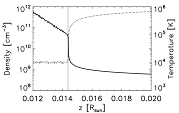
Figure 1: Enlargement of initial vertical profiles of density (continuous line) and temperature (dotted line) in logarithmic scale. The vertical grey line shows the transition region between the chromosphere and the corona.

The accretion stream is assumed to fall along the $z$ axis with a velocity of about $500$ km s^-1 when it impacts onto the chromosphere. The stream is in pressure equilibrium with the surrounding medium and consists of a column with density $10^{9}$ cm^-3 and of a train of consecutive blobs with higher density. The density of the blobs is a free parameter that we change in the simulations. We also performed a simulation describing a continuous accretion stream to provide a baseline case for the simulations of fragmented streams.

Table 1 summerizes the parameters of the simulations: model abbreviation, blob density ($\rho_{bl}$), interblob density ($\rho_{str}$), impact speed ($V_{imp}$), time between two consecutive blobs ($\Delta t_{bl}$), blob length ($R_{bl}$) and accretion rate ($\dot{M}_{acc}$).

In addition to the simulations describing the impact of a train of blobs, we performed simulations describing the more general case of a falling series of circular fragments (blobs) with a random spatial distribution. We assumed the stream consisting of a column with density $10^{9}$ cm^-3 and a series of blobs with random values of density ranging between $5\times 10^{10}$ cm^-3 and $5\times 10^{11}$ cm^-3. For the runs Frag-N20 and Frag-N55 the Table 1 reports the number of blobs described in the initial conditions ($N_{bl}$). For these simulations we adopted a cartesian coordinate system and solved the MHD equations in the plane $(x,y)$. These simulations are analogous to those presented by Reale et al. (2014) except for the presence of the stellar magnetic field which we considered here. This allowed us to compare our results with those presented in Reale et al. (2014) and to evaluate the role of the magnetic field in determining the structure of the post-shock plasma.

Table 1: Parameters of the simulations

Simulation	$\rho_{bl}$	$\rho_{str}$	$V_{imp}$	$\Delta t_{bl}$	$R_{bl}$	$\dot{M}_{acc}$
	($10^{11}$cm-3)	($10^{9}$cm-3)	$10^{7}$cm s-1	(s)	R⊙	$10^{-11}M_{\odot}yr^{-1}$
TR-D11-T300-R10.3	1	1	5	300	0.27	10.3
TR-D11-T150-R10.3	1	1	5	150	0.27	9.3
TR-D11-T600-R10.3	1	1	5	600	0.27	6.14
TR-D11.7-T300-R10.3	5	1	5	300	0.27	50.3
TR-D11-T300-R9.9	1	1	5	300	0.135	5.9
1BL-R10.3	1	1	5	—	0.27	8.6
CONT	—	100	5	0	—	22.5
Simulation	$\rho_{bl}$	$\rho_{str}$	$V_{imp}$	$N_{bl}$	$R_{bl}$	$\dot{M}_{acc}$
					R⊙	$10^{-11}M_{\odot}yr^{-1}$
Frag-N20	0.5-5	1	5	20	0.005 - 0.02	$0.6$
Frag-N55	0.5-5	1	5	55	0.005 - 0.01	$0.55$

The calculations were performed using PLUTO v4.1 (Mignone et al., 2007), a modular, Godunov-type code for astrophysical plasmas. The code is designed to use parallel computers using Message Passage Interface (MPI) libraries. The MHD equations are solved using the MHD module available in PLUTO with the Harten-Lax-van Leer Discontinuities (HLLD) approximate Riemann solver (Miyoshi and Kusano, 2005). The evolution of the magnetic field is calculated using the constrained transport method (Balsara and Spicer, 1999) that maintains the solenoidal condition at machine accuracy. The time evolution is solved using a second order Runge-Kutta method. The radiative losses ${\Lambda}$ are calculated at the temperature of interest using a table lookup/interpolation method. The thermal conduction is treated with a super time-stepping method; the superstep consists of N substeps, properly chosen for optimization and stability, depending on the diffusion coefficient, the grid size and the free parameter $\nu<1$ (Alexiades et al., 1996).

The 2D domain consists of an uniform grid with a cell size of $2.15\times 10^{8}$ cm on the horizontal coordinate ($r$ in cylindrical coordinates and $x$ in cartesian) and $2.69\times 10^{6}$ cm on the vertical coordinate ($z$ in cylindrical, $y$ in cartesian). At the lower boundary we set conditions for density, pressure and temperature to describe the stellar chromosphere; a discontinuous inflow is defined at the upper boundary. In simulations adopting a cylindrical geometry we assumed axisymmetry on the left boundary ($r=0$) and outflow on the right boundary; in simulations adopting a cartesian geometry we used periodic boundary conditions in both the left and right boundaries.

2.1 Synthesis of UV and X-ray emission

From the model results, we synthesized the C IV (1550 Å) and O VIII (18.97 Å) emission lines, both belong to a doublet. First we reconstructed the 3D spatial distributions of plasma density, temperature, and velocity by rotating the 2D spatial domain around the axis of symmetry (i.e. the z axis). We calculated the emission measure of the j-th cell as $EM_{j}(T)=\rho_{j}dV_{j}$, where $dV_{j}$ is the volume of the cell. Then the distribution of emission measure vs. temperature, EM$(T)$, is derived by binning the emission measure values as a function of temperature in the range $[4.5<\log T({\rm K})<7]$; the range of temperature is divided into 30 bins, all equal on a logarithmic scale. From the distributions of emission measure and temperature, we synthesized UV and X-ray spectra, using the CHIANTI atomic lines database (Landi et al., 2013) and assuming solar metal abundances. The spectral synthesis includes the Doppler shift of lines due to plasma motion along the line of sight, we supposed that the angle between the line of sight and the axis of accretion column is 0. We integrated the X-ray and UV spectra from the cells in the whole spatial domain. For each simulation, we summed the spectra derived for the different time frames and divided the resulting spectra by the total time of the simulation. Finally we convolved our high resolution spectra with a Gaussian function of $\sigma$ 17 km s^-1, for C IV profiles, to approximate the spectral resolution of HST observations (Ardila et al. 2013). For O VIII profiles we convolved our high resolution spectra with a Gaussian function of $\sigma$ of 81 km s^-1 to approximate the spectral resolution of Chandra/HETG .

3 Results

3.1 Impact of a train of blobs

We considered as a reference the case of a stream consisting of a train of blobs aligned one to the other with density $\rho=10^{11}$cm^-3, downfalling velocity of $\approx 500$ km s^-1, and with a time interval between two consecutive blobs of $\Delta t=300$ s(run TR-D11-T300-R10.3 in Table 1). The density of the interblob medium is $10^{9}$ cm^-3 in all the simulations. In order to study the effects of stream fragmentation, we performed also a simulation describing a continuous stream with density $\rho=10^{11}$ cm^-3 for comparison.

Initially the evolution of the train of blobs is analogous to that of the continuous stream. Fig. 2 shows maps of temperature and density for our reference case in a time range between 5 and 15 minutes from the beginning of the simulation. Movies showing the complete evolution of 2D spatial distributions of mass density (on the left) and temperature (on the right) in log scale are provided as online material. The train of blobs flows along the magnetic field lines, and the first blob impacts the stellar surface at $t\approx 50$ s at about 500 km s^-1 (Fig. 2a) and sinks into the chromosphere until its ram pressure equals the thermal pressure of the chromosphere.

The collision generates a transmitted and a reverse shock, the latter travels back through the blob and gradually builds up a dense slab of shock-heated plasma at temperatures of few MK (Fig 2b). Given the magnetic field strength ($500$ G) considered in our simulations, the plasma $\beta<<1$ in the slab. As a consequence, mass and energy exchanges across field lines are prevented and the slab is structured in several fibrils, each independent of the others (Sacco et al., 2010). The evolution of each of these fibrils consists of alternating phases of expansion and collapse of the shock-heated plasma (see Sacco et al. 2010). The expansion phase is guided by the reverse shock and ends when the post-shock plasma becomes thermally unstable. Then the system enters in the collapse phase: the catastrophic cooling robs the post-shock plasma of pressure support, causing the collapse of the material above. After the fibril has disappeared in chromosphere, a new fibril is re-built by the reverse shock. During the evolution, the thermal conduction continuously drains energy from the shock-heated plasma to the chromosphere, thus acting as an additional cooling mechanism of the hot slab (see also Orlando et al. (2010)). At the same time, the conduction contrasts the radiative cooling. The heat flux saturation (see Eqs. 2) limits the effects of thermal conduction where temperature gradients are very steep, in particular at the contact discontinuity between the chromosphere and the hot slab and in regions affected by catastrophic cooling of dense plasma.

The evolution of the train of blobs departs from that of the continuous stream when the reflected shock reaches the upper boundary of the blob (Fig. 2b). At that time, the pressure of the shocked blob is much higher than the ram pressure of the layers above due to the low density of the interblob region. As a result the hot and dense plasma of the shocked blob expands adiabatically upward through the accretion column. During this phase the shock-heated plasma gradually cools down as a result of the adiabatic expansion. The expansion ends when the upflowing surge collides with the following blob generating a second shock region high in the accretion column (h=0.1$R_{\odot}$) (Fig. 2d, e). In this phase the blob plasma can reach temperatures up to $10^{7}$ K. This shock region is dragged down by the blob at velocities of $\approx 500$ km s^-1 until it impacts the chromosphere and sinks (Fig. 2f). Then a new shock develops and travels through the blob, re-building the hot slab.

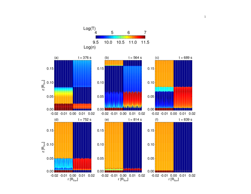
Figure 2: Color maps in log scale of evolution of density (left half-panel) and temperature (right half-panel) of plasma for the reference case (run TR-D11-T300-R10.3 in Table1). White lines represent magnetic field lines.

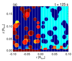
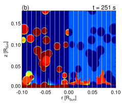
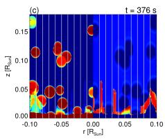
Figure 3: Color maps in log scale of evolution of density (left half-panel) and temperature (right half-panel) of plasma for the general case of fragmented stream (run Frag-55 in Table 1). White lines represent magnetic field lines.

3.2 Exploration of the parameter space

For the model describing a train of blobs, we performed an exploration of the parameter space defined by three free parameters (see Table 1): the frequency of blobs (or, in other words, the distance between two consecutive blobs), the size of the blobs, and the density of the blobs. The aim is to evaluate how a different fragmentation changes the structure of the post-shock region and the observables (namely the distribution of emission measure vs. temperature and the line profiles). Note that the different parameter determine a different accretion rate (see Table 1).

The effect of the blob frequency was investigated by comparing the reference case (run TR-D11-T300-R10.3) to two additional simulations: one with half a distance between two consecutive blobs (run TR-D11-T150-R10.3), and the other with twice a distance (run TR-D11-T600-R10.3). The density of the blobs is the same as in the reference simulation. As in the reference case, the blob impacts produce upflowing surges that hit the subsequent downfalling blobs. In the simulation TR-D11-T150-R10.3 the interaction of the surging upflow with the blob occurs closer to the stellar surface (h= 0.08$R_{\odot}$) than in the reference case due to the smaller distance between two consecutive blobs. The interaction produces a shock in the downfalling blob with temperature of $10^{7}K$. This shocked plasma flows downward with speeds of $\approx$ 300 km s^-1. In the case TR-D11-T600-R10.3 the surging upflows have more time to move upwards and cool down before hitting the subsequent blobs. In this case the impact occurs at distances from the stellar surface (h= 0.27$R_{\odot}$) larger than in the reference case. As a result, the post-shock region is more extended above the chromosphere and is characterized by a large range in plasma temperature (from $10^{4}$ to $10^{7}$ K) and by plasma with downfalling velocities of $\approx$ 250-300 km s^-1.

We explored the effect of the size of the blobs on the evolution and structure of the post-shock plasma by comparing the reference case with a simulation of blobs with a smaller size (run TR-D11-T300-R9.9). In the latter case the upflowing surges developed earlier and therefore occur more frequently than in the reference case due to the smaller size of the blobs. The temperature of the post-shock region is $\approx 8\times 10^{6}$ K and the surges hit the subsequent blobs at $\approx 0.14R_{\odot}$. The structure of the post-shock plasma is analogous to that of the reference case: the impacts of upflowing surges and downfalling blobs generate shocks with temperature of $\approx 10^{7}$K and plasma which fall down with velocities of $\approx$ 150-300 km s^-1.

The effect of blob density on the structure of the post-shock region was investigated by comparing the reference case with a simulation assuming denser blobs ($\rho=5\times 10^{11}$ cm^-3; run TR-D11.7-T300-R10.3). The density of the interblob region and the blob frequency are the same as those of the reference case. As expected, denser blobs penetrate more deeply in the chromosphere due to their higher ram pressure and the stand-off height of the shocks transmitted in the blobs is smaller than that in the reference case (see Sacco et al. 2010). Again upflowing surges develop after the shocks reach the upper boundary of the blobs and hit the following blobs generating plasma with temperature up to $\approx 10^{7}$K. The structure of the post-shock region is analogous to that found in the other simulations and is characterized by plasma with temperatures in the range between $10^{4}$ and $10^{7}$ K and downfalling velocities of $\approx$ 300-400 km s^-1.

Finally, just as a guide, we performed an additional simulation describing the impact of a single blob with density $\rho=10^{11}$cm^-3, downfalling velocity 500 km s^-1, and size $1.87\times 10^{10}$ cm (run 1BL-R10.3). This simulation can be considered as an extreme case in which the time between two consecutive blobs is much larger than the duration of observation. In this case, after the impact of the blob with the chromosphere, the resulting surge expands upward without any interaction with downfalling blobs. The post-shock plasma cools down rapidly and is expected to produce blueshift of emission lines to speeds around $\approx$ 400 km s^-1.

3.3 Randomly fragmented stream

The more general case of a randomly fragmented stream was investigated through simulations describing a column with uniform density of $10^{9}$ cm^-3 and a series of circular blobs with random spatial distribution and random density in the range $5\times 10^{10}$ and $5\times 10^{11}$ cm^-3.

In these simulations, the blob impacts reproduce all the cases explored assuming a train of blobs and, in addition, consider the interaction of multiple shocks with downfalling fragments. We performed two simulations assuming the same mass accretion rate but with different granularity of stream fragmentation: run Frag-N20 considers 20 blobs with radius ranging between $3.48\times 10^{8}$ cm and $1.39\times 10^{9}$ cm (coarse fragmentation), and run Frag-N55 considers 55 blobs with radius ranging between $3.48\times 10^{8}$ cm and $6.96\times 10^{8}$ cm (fine fragmentation).

The evolution is quite similar in the two cases. As for the train of blobs (see Sect. 3.1), the first blobs impact onto the chromosphere and produce upflowing surges of post-shock plasma that expand through the interblob medium (see Fig. 3 and on-line movie). The expansion ends when the surges hit the following falling blobs. At variance with the case of a train of blobs, the interactions of the surges with the falling blobs occur at different altitudes due to the initial random positions of the blobs in the stream. As a result, the structure of the post-shock region is very complex and consists of several knots and filaments of shock-heated plasma with a broad range of velocities, densities, and temperatures (see Fig. 3). The two runs Frag-N20 and Frag-N55 differ mainly for the average extension of the post-shock region. In fact, in run Frag-N20 the average distance among the blobs is larger than that in run Frag-N55. As a consequence, the surges have more time to expand upwards, so that their interactions with the downfalling blobs occur, on average, at higher altitudes. Because of this longer expansion, we also expect that a plasma component contributing to a blue shift of emission lines (namely that due to the upflowing surges) would be more important in run Frag-N20 than in run Frag-N55.

Our case of a randomly fragmented stream is similar to the HD model developed by Reale et al. (2014). The main differences are that the latter, neglect the magnetic field and consider blobs with not perfectly vertical trajectory with respect to the chromosphere. As a result, in the case explored by Reale et al. (2014), the plasma dynamics is not influenced by the magnetic field lines and the small deviation from the vertical trajectory determines an asymmetric evolution of the post-shock plasma. The surges that bounce back are not confined by the magnetic field and are free to expand upward and laterally, causing a more efficient adiabatic cooling of the plasma and a lower upflowing velocity. Also the inclined trajectory of the blobs causes the surges to develop preferentially in the direction opposite to that of arrival of the blobs. For all of these reasons the post-shock region is very complex and characterized by a wide range of velocities of the shocked plasma.

3.4 Distribution of emission measure vs temperature

The distribution of emission measure versus temperature, EM(T), is a source of information of the plasma components with different temperature contributing to the emission. In particular, we are interested on the components with temperatures $\log(T)\approx 5$ K, responsible of the C IV line emission, and with $\log(T)\approx 6.5$ K, contributing to the O VIII line.

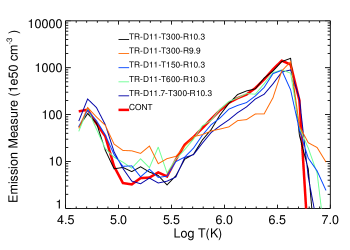
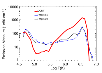
Figure 4: Distributions of emission measure vs temperature normalized to the accretion rate of TW Hya. The upper panel shows the distributions derived for a train of blobs and for a continuous stream; the lower panel shows the distributions derived for the general case of a fragmented stream.

From the model results, we derived the EM$(T)$ distributions, following the methodology outlined in Sect. 2.1. The distributions are obtained for all the frames of our simulations and then averaged over the time covered by the simulations. Then they are rescaled to a mass accretion rate of $10^{-9.17}$M_⊙ yr^-1 in agreement with optical observations of TW Hya (Curran et al., 2011). The upper panel of Fig. 4 shows the result for the trains of blobs. All these EM$(T)$ distributions have a shape similar to that of the continuous stream (red curve in the figure) and show two peaks, one at $\log T(K)\approx 4.7$ and the other at $\log T(K)\approx 6.5$. The former is due to the shocked plasma that cools down catastrophycally, the latter to the shock-heated plasma (see also Sacco et al. 2010). The distributions also present a pronounced dip at $\log T(K)\approx 5-5.5$ (namely in the range of temperatures where the radiative losses are more efficient) in which the EM can be up to 2 orders of magnitude lower than that at $\log T(K)\approx 6.5$. By comparing the simulations of the train of blobs with that describing a continuous stream, we note that the former in general have larger emission measure in the range of temperatures between $\log T(K)\approx 5$ and $\log T(K)\approx 5.5$ and smaller emission measure at $\log T(K)\approx 6.5$ than the continuous case.

The lower panel of Fig. 4 shows the EM$(T)$ distributions derived from the simulations describing the randomly fragmented stream (runs Frag-N20 and Frag-N55). Again the distributions present two peaks at $\log T(K)\approx 4.7$ and $\log T(K)\approx 6.5$. But the distributions are flatter in the temperature range between $\log T(K)\approx 5$ and $\log T(K)\approx 6.5$, and the dip at $\log T(K)\approx 5.5$ is shallower to less than one order of magnitude from the peak at $\log T(K)\approx 6.5$. In fact, in these simulations, the fine stream fragmentation makes the impact frequency higher than in the case of a train of blobs. As a result, the post-shock region is quite complex and characterized by several structures of shock-heated plasma interacting each other and with a broad range of densities and temperatures (see Sect. 3.3). Even if the radiative losses are very efficient around $\log T(K)\approx 5$, several plasma structures which cool down are present at the same time in that range of temperatures thus contributing to increase the EM(T) values there.

3.5 UV and X-ray emission

From the model results, we synthesized the emission in the UV and X-ray bands (see the method outlined in Sect. 2.1), focusing our analysis on the doublets of C IV (1550 Å) and O VIII (18.97 Å). In all the cases, we assume that the line of sight is aligned with the stream axis, thus maximizing the line shifts. Figure 5 shows the profiles of the C IV doublet derived from models with trains of blobs. The line profile derived from the model of a continuous stream is also overplotted for comparison (red curve). Note that the line profiles are convolved with a Gaussian of $\sigma$ 17 km s^-1 (for C IV) to approximate the spectral resolution of HST (Ardila et al., 2013) observations. and 81 km s^-1 (for O VIII) to approximate the spectral resolution of Chandra/HETG.

In the case of a continuous stream, the C IV line profile is characterized by a prominent slow component (hereafter SC) with a net redshift of $\approx 50$ km s^-1 and by a second less intense and faster component (hereafter FC) with a redshift of $\approx 250$ km s^-1. The former originates from the base of the accretion column close to the stellar chromosphere where the post-shock plasma cools down under the effect of thermal conduction and radiative losses and decelerates from $\approx 120$ to few km s^-1. The FC originates from catastrophic cooling of dense plasma accelerated to velocities around 200-250 km s^-1 by the downfalling plasma above. We note also that the simulation of a single blob (run 1BL-R10.3) shows a profile analogous to that of a continuous stream. As for the latter, in fact, the contribution to the C IV line originates mainly from the cooling plasma at the base of the blob (responsible of the SC) and from the post-shock plasma subject to catastrophic cooling (responsible of the FC).

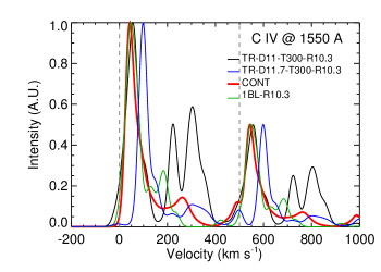
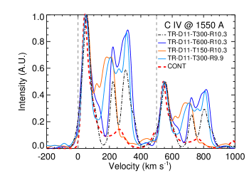
Figure 5: Synthetic profiles of C IV doublet; all the profiles are normalized to their maximum value. The upper panel compares our reference simulation of a train of blobs (run TR-D11-T300-R10.3) with the case of a continuous stream (run CONT), the case of a single downfalling blob (run 1BL-R10.3), and with the case of a train of blobs with higher density (run TR-D11.7-T300-R10.3). The lower panel compares profiles derived from simulations of a train of blobs differing for the frequency and size of blobs (runs TR-D11-T300-R10.3, TR-D11-T600-R10.3, TR-D11-T150-R10.3, TR-D11-T300-R9.9). The dotted grey lines are the rest positions of the lines of the doublet.

For a train of blobs, the line profiles are much more complex than for a continuous stream due to the more structured post-shock region. The lines exhibit broadening and asymmetries reflecting the plasma structures with different downfalling velocities present in the post-shock region. As for the case of a continuous stream, all the lines are characterized by a SC. Again this component is due to post-shock plasma which cools down and decelerates at the base of the accretion column. The main differences with the case of a continuous stream are in the FC. In the train of blobs, the FC can be large with intensity even comparable with that of the SC. In general the FC is split into multiple components with redshift ranging between 200 and 400 km s^-1 (see Fig. 5). These components originate from the interaction of upflowing surges with downfalling blobs and from plasma subject to catastrophic cooling induced by radiative losses (see $\Lambda(T)$ in Eq.3) , as in the case of a continuous stream . Our simulations show that the relative intensity of the FC increases when the surges have more time to expand upward (for instance in runs TR-D11-T600-R10.3 and TR-D11-T300-R9.9), suggesting that the finer the fragmentation, the higher is the intensity of the FC. Also we note that the FC is broader for the train of blobs than for the continuous stream because of the larger range of velocities of plasma structures contributing to C IV emission in the former case. Finally we note that both the SC and FC are more redshifted for higher density of the blobs (see upper panel in Fig. 5) and the FC is less intense than in the other cases.

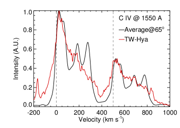
Figure 6: Comparison between the synthetic profile of C IV doublet resulting from summing all the line profiles derived from the simulations of a train of blobs (black) and the observed spectrum of TW Hya analyzed by Ardila et al. (2013) (red). We assumed an angle between the line of sigth and the axis of the accretion column of 65 degrees to fit the velocity shift of the peak emission of the observed line. The profiles are normalized to their maximum value. The dotted grey lines represent the rest positions of the doublet.

From all the simulations of a train of blobs, we derived the synthetic C IV line profile resulting from summing all the line profiles normalized to the accretion rate of TW Hya. This profile is expected either from a single accretion stream consisting of a train of blobs with different size and density or from few streams each with different train of blobs and accreting onto the CTTS at the same time. In Fig. 6 we compare this synthetic C IV line profile with the profile observed from TW Hya and analyzed by Ardila et al. (2013) both normalized to their maximum. We also assumed an angle of 65 degrees between the line of sight and the axis of the accretion column to fit the velocity shift of the emission maximum of the observed profile. This angle is in good agreement with that suggested in the literature (e.g. Ardila et al. 2013). The synthetic profile can be described by three main components: a narrow slow component with a redshift of $\approx 50$ km s^-1 and two faster components with a redshift ranging between $200$ and $250$ km s^-1. Note that the observed profile shows only one broad fast component that we interpret as the envelope of several fast components (see below). In general, we found that the synthetic profile reproduces the asymmetries observed in the profile from TW Hya. The slow component in the synthetic profile should correspond to the observed narrow component found by Ardila et al. (2013) (see Fig. 6). The two faster components may explain the origin of the observed broad component. This is especially true if we consider that, in a more realistic scenario, few accretion streams with different viewing angles (and therefore different line shifts) might coexist, so that the two faster components would be broader and possibly merge into a single broad fast component.

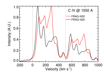
Figure 7: As in Fig. 5 for the general case of a fragmented stream (runs Frag-N20 and Frag-N55).

Fig. 7 shows the synthetic line profiles derived from the randomly fragmented stream (runs Frag-N20 and Frag-N55). As for the train of blobs, The line profiles are still characterized by a narrow SC at $\approx 100$ km s^-1 due to the cooling plasma at the base of the accretion column. In the general case, however, the profiles are more complex than for the train of blobs and show several fast components with redshift ranging between 200 and 400 km s^-1. Such a complexity is due to the structure of the post-shock region which consists of several knots and filaments, possibly subject to radiative cooling, with a broad range of velocities. As expected in the light of the results obtained for a train of blobs, the high level of stream fragmentation increases the relative intensity of the faster components. An extreme case is run Frag-N55 in which the most prominent component is at $\approx 300$ km s^-1. In fact, as also discussed in Sect. 3.4, the larger is the number of blobs with different density and size, the more frequent the interactions of upflowing surges with downfalling blobs, and the larger the number of structures of shock-heated plasma with a broad range of densities, velocities and temperatures. Many of these structures cool down under the effect of radiative losses, thus contributing to the emission of the C IV doublet.

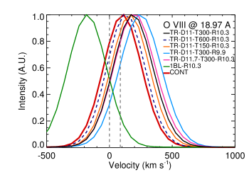
Figure 8: Synthetic profile of O VIII doublet normalized to their maximum value for the simulations of a train of blobs, the simulation of a single blob, and the case of a continuous stream. The dotted grey lines represent the rest positions of the doublet.

From the models, we synthesized also the O VIII doublet in the soft X-ray band. Figure 8 shows the line profiles for the simulations of a train of blobs and for a continuous stream, assuming again the line-of-sight aligned with the stream axis. For O VIII, the profiles are simpler than those of C IV mainly because of the lower spectral resolution of available X-ray instruments. However, despite the low resolution, some information can be obtained from the analysis of O VIII lines. In fact, the figure clearly shows that, in principle, a net redshift due to the accretion process is detectable, depending on line S/N, and viewing direction. The case of a continuous stream (red curve in the figure) presents the lines with the minimum redshift, with a velocity of $\approx 100$ km s^-1, compatible with the post-shock velocity. The simulations of a train of blobs present higher redshifts because of the contribution of hot plasma at the interaction region between the upflowing surges and the downfalling blobs. The redshift increases roughly with the level of stream fragmentation; the highest redshift is found for run TR-D11-T300-R9.9, namely the case assuming smaller blobs. Finally, a net blueshift ($\approx 200$ km s^-1) is found for the case of a single blob (run 1BL-R10.3), for which the emission arises mainly from the post-shock plasma free to expand upward. It should be noted, however, that the line intensity derived for this case is more than one order of magnitude lower than those derived in the other cases (Fig. 8 shows intensities normalized to the maximum).

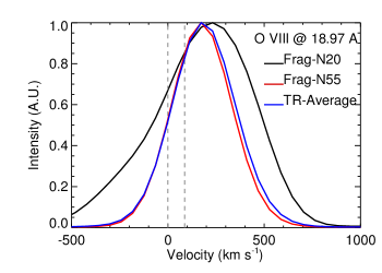
Figure 9: As in Fig. 8 for the randomly fragmented stream (runs Frag-N20 and Frag-N55). TR-Average is the average line profile obtained from the train of blobs simulations.

The O VIII doublets synthesized for the case of a randomly fragmented stream (runs Frag-N20 and Frag-N55) are shown in Fig. 9. The results of run Frag-N55 are similar to those derived for the train of blobs. The line appears symmetric and redshifted to speed of $\approx 200$ km s^-1. The profile almost superimpose to that obtained summing all the spectra derived from the simulations of a train of blobs (blue curve in Fig. 9). On the contrary, the line profile synthesized from run Frag-N20 is asymmetric (with an intense and extended blue wing) and broader than in run Frag-N55. We note that the blobs in run Frag-N20 are sparser than in run Frag-N55. As a result, the surges have more time to expand upward without impacts with downfalling blobs, thus contributing more to the blue wing of the O VIII line.

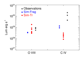
Figure 10: Luminosity of C IV and O VIII lines synthesized from the models for the case of a train of blobs (red dots; Sim-Tr) and for the case of randomly fragmented stream (blue dot; Sim-Frag). The luminosity derived from UV and X-ray observations of three well-studied CTTSs are superimposed (black dots; MP Mus, Argiroffi et al. 2007; TW Hya, Brickhouse et al. 2010; V4046 Sgr, Argiroffi et al. 2012).

Finally, we derived the luminosity of C IV and O VIII doublets from all our simulations and compared the synthetic values with those derived from UV and X-ray observations of three well-studied CTTSs, namely MP Mus (Argiroffi et al. 2007), TW Hya (Brickhouse et al. 2010), and V4046 Sgr (Argiroffi et al. 2012). The results of our simulations and the comparison with observations are shown in Fig. 10. The models are normalized in order to have a mass accretion rate of $10^{(-9.17)}$ M_⊙ yr^-1 (namely comparable with those inferred from optical observations of TW Hya; Curran et al. 2010). We found that, in general, our models reproduce quite well the order of magnitude of the observed O VIII luminosity. This was expected for the case of a continuous stream (Sacco et al., 2010); we show that models of fragmented streams predict luminosities of the O VIII doublet a bit lower than those for models of continuous streams. On the other hand, we found that models of a train of blobs predict C IV luminosities significantly lower than those observed, although they are in better agreement with the observations than models of a continuous stream (see Fig. 10). Recently Costa et al. (2016, submitted) have proved that such a discrepancy may be reconciled if the effect of the radiative heating of the infalling material by the post-shock plasma is taken into account in the models. Nevertheless, it is interesting to note that, in the case of highly fragmented streams (runs Frag-N20 and Frag-N55), our model predict C IV luminosities significantly higher than those found by a train of blobs. Inspecting Fig. 10 we note that normalizing the X-ray luminosity synthesized from runs Frag-N20 and Frag-N55 to observations also the UV luminosity synthesized by the same models is shifted at higher values, thus providing a better agreement. (see Fig. 10). This is also in agreement with the results of Sect. 3.4: the EM$(T)$ distributions are characterized by a lower dip at $\log(T)\approx 5$ K (namely around the temperature of formation of the C IV doublet) if the stream is highly fragmented. In fact, in these cases, a variety of plasma structures with different density and temperature characterizes the post-shock region, most of them cool down because of radiative losses and contribute to the emission of the C IV doublet. We suggest that a high stream fragmentation may contribute to increase the UV emission of accretion impacts.

4 Summary and conclusions

In this work we investigated the effects of stream fragmentation on C IV and O VIII emission lines. We developed a model that describes a stream composed by a series of dense blobs impacting onto the surface of a CTTS. Our model takes into account the stellar magnetic field, the gravity, the radiative losses from optically thin plasma and the thermal conduction. The aim was to explore if and how the impact of a fragmented stream onto the chromosphere of a CTTS reproduces profiles of C IV doublet similar to those observed by Ardila et al. (2013). Our main findings can be summarized as follow:

• The impact of a series of dense blobs onto the stellar surface produces a more complex post-shock region than that in the case of a continuous stream. In particular the blob impacts produce strong shocks propagating through the blobs and then upflows after the blobs are fully shocked. The upflows in turn hit and shock the still downfalling blobs, producing a large variety of plasma structures (knots, filaments) differing in density, temperature, and downfalling velocity. These structures are not present in the case of a continuous stream.

• If the stream is fragmented the C IV (1550 Å) lines have a highly asymmetric and broad profiles. The lines split into a narrow and intense component redshifted to speed $\approx 50$ km s^-1 and a multitude of faster components redshifted to speeds in the range between 200 and 400 km s^-1. The narrow component originates from the post-shock plasma at the base of the accretion column which cools down under the effect of thermal conduction and radiative losses. The fast components originate from thermal instabilities occurring at high altitudes in the shocked stream and from the plasma structures forming during the interaction of upflowing surges and downfalling blobs. This is in agreement with Reale et al. (2014).

• The intensity and velocity of the fast components depend on the stream fragmentation: the finer is the fragmentation, the more intense are the fast components. Assuming a more realistic scenario in which few accretion streams with different viewing angles (and therefore different line shifts) are present, the fast components easily merge together to form a single broad component redshifted to speed $\approx 250$ km s^-1. A similar result has been found by Reale et al. (2014) by adopting an HD model to study blob falls on the solar surface. The narrow component at $\approx 50$ km s^-1 and the broad component at $\approx 250$ km s^-1 are analogous to those found by Ardila et al. (2013) for most of the CTTSs of their sample. Thus we interpret the shape of observed C IV lines as evidence of density structured or fragmented accretion streams.

• The O VIII (18.97 Å) lines have a symmetric observable profile redshifted to speed ranging between 100 and 200 km s^-1. The redshift increases roughly with the level of stream fragmentation: the shift is the smallest in the case of a continuous flow and the largest for a train of small blobs. In any case our model predicts that accretion impacts would produce detectable shifts in the O VIII lines.

• As in the case of continuous accretion streams, models of fragmented streams reproduce quite well the luminosity of O VIII lines measured in CTTSs (Argiroffi et al., 2007; Brickhouse et al., 2010; Argiroffi et al., 2012) and, in general, underestimate even by orders of magnitude the luminosity of C IV lines. On the other hand, we found that assuming an high level of stream fragmentation is in better agreement with observations. In these models, in fact, many interactions between upflowing surges and downfalling blobs are present which produce a multitude of plasma structures with different density and temperature. Many of them cool down because of radiative losses thus contributing to emission in C IV lines. We conclude that the stream fragmentation enhances the emission in the UV band.

In conclusion, our models reproduce profiles of C IV and O VIII lines remarkably similar to those observed (Ardila et al. 2013, Argiroffi in preparation) and suggest that the UV emission originates mainly from plasma structures developed as a result of the impact of a density structured or fragmented accretion stream. On the other hand our models predict in general UV luminosities lower than observed. We note that oru models assume that the plasma is optically thin in the whole domain. However, optically thick plasma, as that of the chromosphere and of the unshocked stream, is present around the impact region. This plasma, on one hand, absorb part of the X-ray emission arising from the post-shock plasma (Sacco et al., 2010; Bonito et al., 2014) and, on the other hand, can be heated up to $\log T(K)\approx 5$ by irradiation by the post-shock plasma, thus contributing to UV emission (Costa et al. 2016, submitted). In this work we did not take into account the absorption by optically thick material and the effect of radiative heating of the unshocked stream by post-shock plasma. In a future work we plan to include these effects on the model to investigate more deeply the origin of UV emission arising from impact regions of fragmented accretion streams.