Equation-free analysis of a dynamically evolving multigraph

Abstract

In order to illustrate the adaptation of traditional continuum numerical techniques to the study of complex network systems, we use the equation-free framework to analyze a dynamically evolving multigraph. This approach is based on coupling short intervals of direct dynamic network simulation with appropriately-defined lifting and restriction operators, mapping the detailed network description to suitable macroscopic (coarse-grained) variables and back. This enables the acceleration of direct simulations through Coarse Projective Integration (CPI), as well as the identification of coarse stationary states via a Newton-GMRES method. We also demonstrate the use of data-mining, both linear (principal component analysis, PCA) and nonlinear (diffusion maps, DMAPS) to determine good macroscopic variables (observables) through which one can coarse-grain the model. These results suggest methods for decreasing simulation times of dynamic real-world systems such as epidemiological network models. Additionally, the data-mining techniques could be applied to a diverse class of problems to search for a succint, low-dimensional description of the system in a small number of variables.

1 Introduction

Over the past decades, complex networks have been used as the model of choice for a truly broad class of physical problems, ranging from highway traffic joubert_large-scale_2010 to brain connectivity hermundstad_learning_2011 . When modeling such systems, dynamics are typically defined at a very detailed, “fine” scale, specifying individual node and edge interactions; explicit closed equations governing network macroscopic (collective) properties are often unavailable durrett_graph_2012 ; joubert_large-scale_2010 ; roche_agent-based_2011 ; swaminathan_modeling_1998 . The detailed interactions are often complicated functions dependent on multiple system parameters, which, when one also accounts for large network sizes inherent in many interesting problems, can make systematic numerical exploration computationally prohibitive. The lack of explicit macroscopic equations prohibits the use of traditional numerical techniques such as fixed-point computation and stability analysis, that could offer valuable insight into the network’s behavior, leaving little alternative but to work with full direct simulations of the entire network. Faced with these inherent limitations, investigators must either restrict their attention to a more modest parameter space hodgkin_quantitative_1952 or simplify the network model, potentially removing important features brown_variability_1999 .

Equation-free modeling offers a promise to circumvent these challenges, allowing one to investigate the complex network at a macroscopic level while retaining the effects of full system details kevrekidis_equation-free:_2004 ; gear_equation-free_2003 . Underlying this method is the assumption that, although we cannot analytically derive equations governing network evolution, such closed equations do, in principle, exist. Furthermore, these unavailable equations are assumed to involve a small number of dominant collective (coarse-grained) variables. The important features of the complete network can be in fact, by this assumption, well represented by these select observable quantities. This may seem too restrictive, yet it is exactly the behavior witnessed across many network types: despite the initial complexity of the full system configuration, certain collective network properties appear to evolve smoothly in time, while the evolution of other, “secondary” properties, can be strongly correlated with that of the few “primary” variables bold_equation-free_2014 ; rajendran_coarse_2011 ; siettos_equation-free_2011 . Once these significant variables are uncovered, we can combine short intervals of full system simulation with operators that map the full system description to and from its representative coarse variable “summary”, thus enabling previously-infeasible system-level analysis (see Section 3 for further details).

Here, we apply this framework to a dynamically evolving multigraph model. This offers a test of the methodology in the previously unexplored context of multigraphs. We demonstrate the acceleration of direct network simulations through Coarse Projective Integration (CPI), and the location of coarse stationary states through a matrix-free Newton-GMRES method. In addition, principal component analysis (PCA) and diffusion maps (DMAPS), two well established dimensionality-reduction techniques, are shown to enable an algorithm for characterization of the underlying low-dimensional behavior of the system.

The paper is organized as follows: we begin in Section 2 with a description of the multigraph dynamic model. Sections 3 and 4 provide most details of the equation-free approach, specify how it was applied to our system, and present subsequent results. Section 5 summarizes our use of PCA and DMAPS, and assesses their effectiveness in analyzing hidden, low-dimensional structure in this network system.

2 Model description

We study the edge-conservative preferential attachment model, a detailed mathematical analysis of which can be found in rath_time_2012 and rath_multigraph_2012 . The system evolves in discrete steps $t=0,1,\ldots t_{f}$, and we denote the $n$-vertex graph at each point by $G_{n}(t)$. The initial state, $G_{n}(0)$, is an arbitrary distribution of $m$ edges among the $n$ vertices; the total number of both edges and vertices is conserved. No restrictions are placed on this initial distribution: multiple edges and loops are permitted. The system is then advanced step-by-step based on the following procedure:

1. Choose an edge $e_{ij}\in E(G)$ uniformly at random, and flip a coin to label one of the ends as $v_{i}$

2. Choose a vertex $v_{k}$ using linear preferential attachment: $P(v_{k}=v_{l})=\frac{d_{l}+\kappa}{\sum\limits_{i=1}^{n}d_{i}+n\kappa}$

3. Replace $e_{ij}$ with $e_{ik}$,

where $d_{i}$ is the degree of vertex $v_{i}$, $E(G)$ is the set of edges in the graph, and $\kappa\in(0,\infty)$ is a model parameter affecting the influence degrees have on the probability distribution in Step 2. That is, taking $\lim\limits{\kappa\rightarrow 0}$, we recover “pure” preferential attachment, and probability scales directly with degree, while $\lim\limits_{\kappa\rightarrow\infty}P(v_{k}=v_{l})=\frac{1}{n}\;\forall\;l$, and individual degrees have no effect. A single step of this evolution process is illustrated in Fig. (1). Note that this can also be represented as a graph in which only one edge is permitted between each pair of nodes, but with edge weights signifying the number, or strength, of connections between nodes.

Evolving the system in this manner, the degree sequence approaches a stationary distribution over $O(n^{3})$ steps. As explained in rath_time_2012 , this distribution is dependent only on the system parameters $\rho=\frac{2*m}{n}$ and $\kappa$. Fig. (2) illustrates the evolution of the degree sequence of two networks with different initial configurations but the same values of $\rho$ and $\kappa$ respectively; as expected, we observe they approach an identical stationary state.

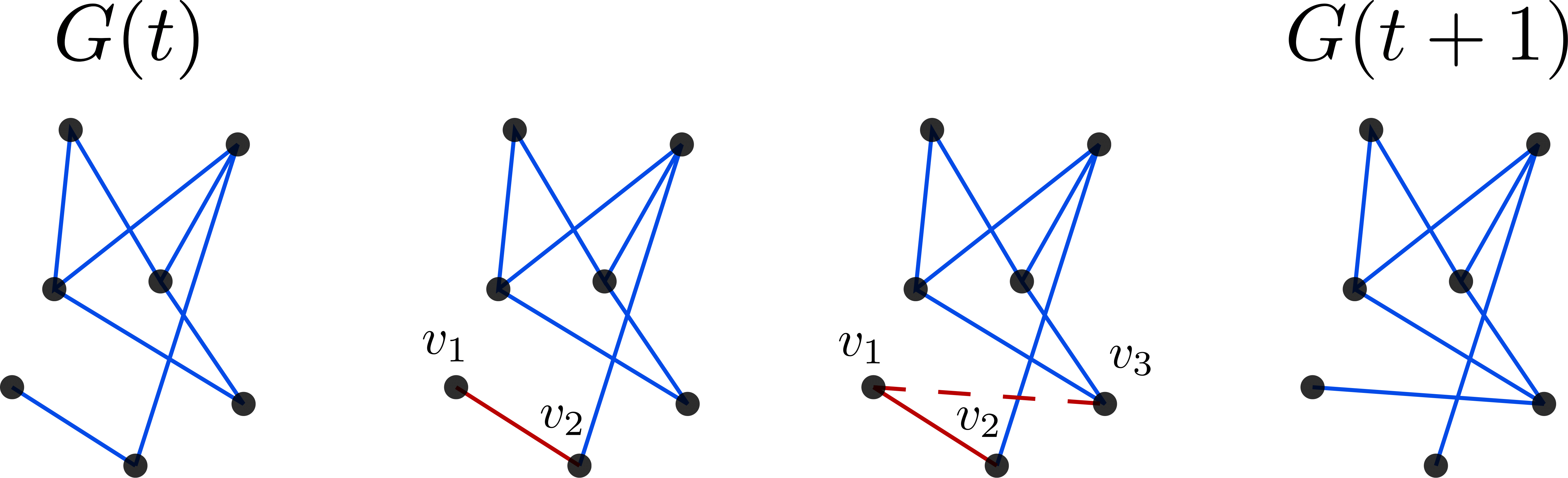
Figure 1: Schematic of the substeps of the evolution dynamics of the multigraph $G(t)$.

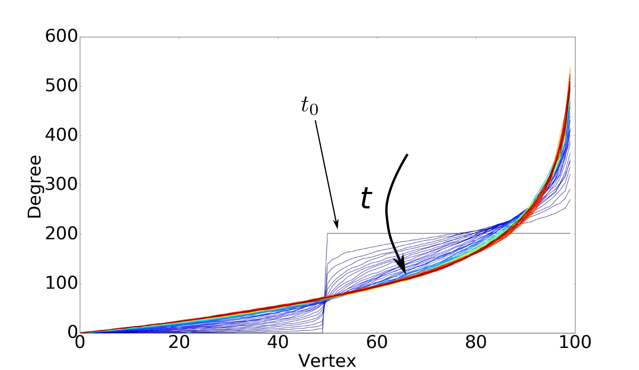
(a)

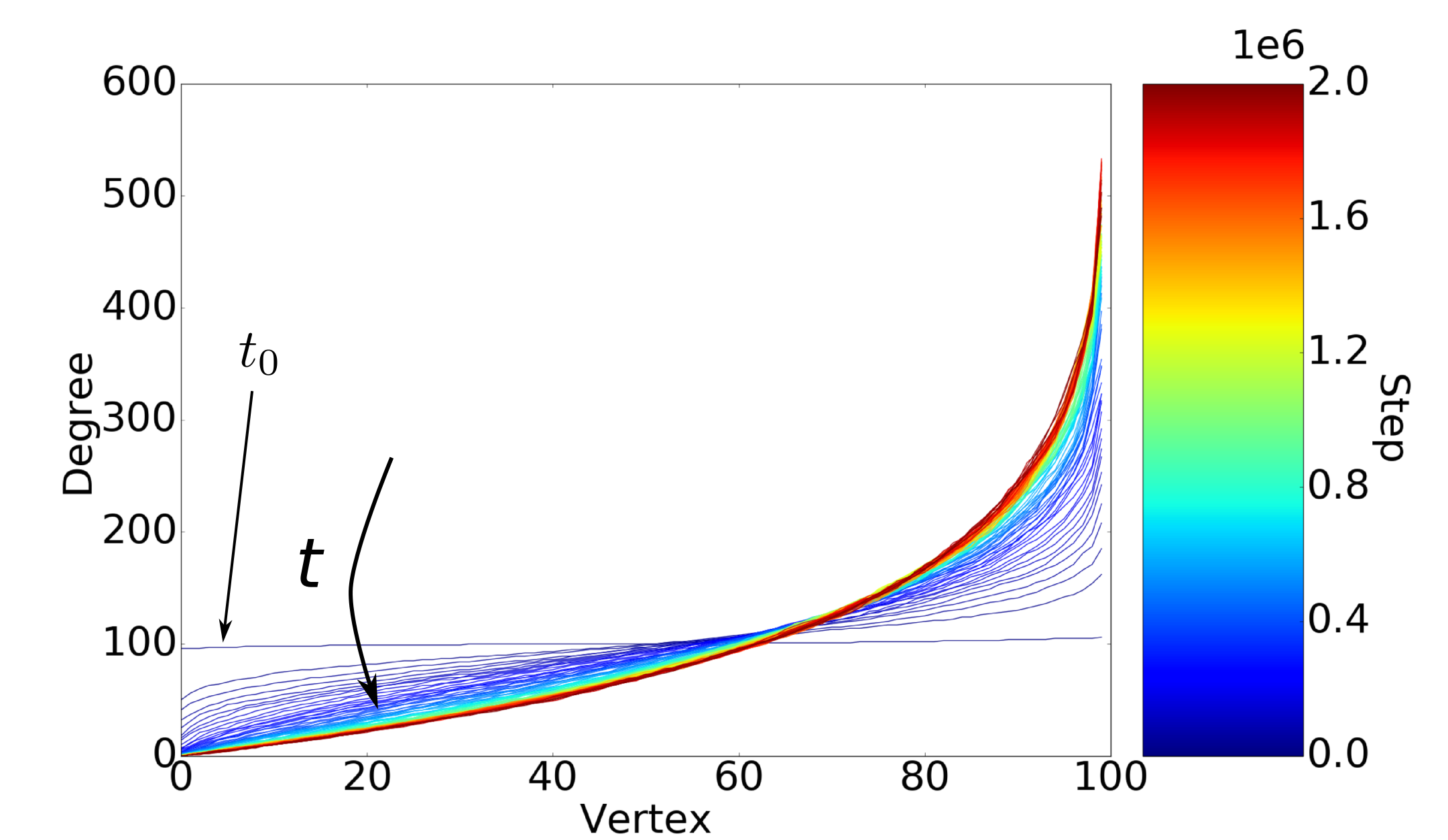
(b)

Figure 2: Evolution of the multigraph model’s sorted degree sequence. Two distinct transients are shown, initialized with (a) an Erdős-Rényi random graph with $m=5,050$ edges and (b) a graph in which half the vertices are isolated, and half uniformly share $m=5,050$ edges. Both approach the same ultimate stationary sequence. To smoothen the evolution of this stochastic system, here we plot the instantaneous average of twenty simulations.

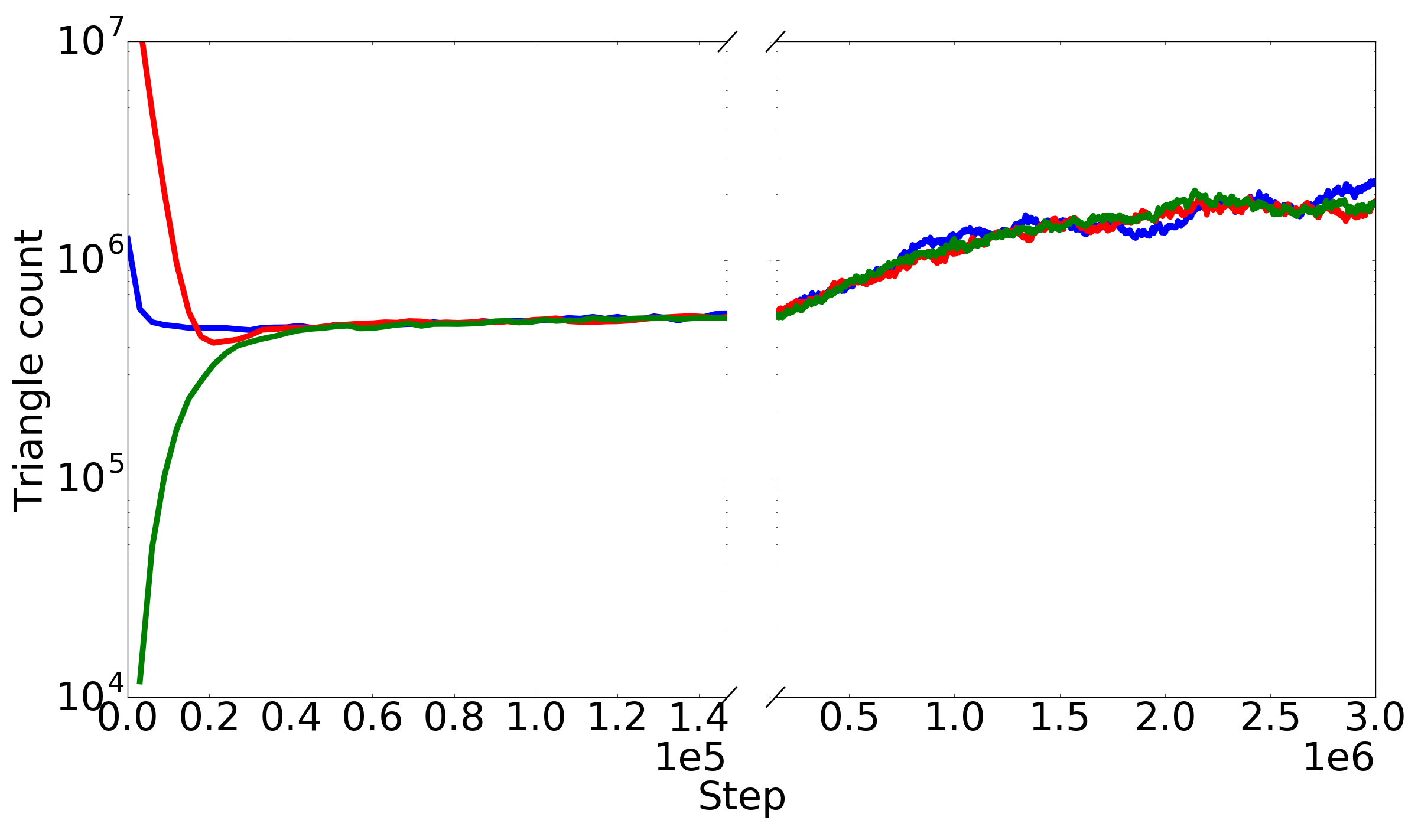
Figure 3: Evolution of higher-order network statistics (here, the total triangle count) for three different network initializations. They are quickly ($O(n^{2})$ steps) drawn to a slow manifold on which they slowly evolve over ($O(n^{3})$ steps) to a stationary state.

3 Equation-free modeling

3.1 Coarse-graining

A prerequisite to the implementation of equation-free algorithms is the determination of those few, select variables with which one can “close” a useful approximate description of the coarse-grained dynamics of the full, detailed network. This set of variables should clearly be (much) less than those of the full system state, and they should evolve smoothly (so, either our network would have a large number of nodes, or we would take expectations over several realizations of networks with the same collective features). Based on the profiles depicted in Fig. (2), the graph’s degree sequence, (equally informatively, its degree distribution) is a good candidate collective observable. It appears to evolve smoothly, while also providing significant savings in dimensionality, from an $O(n^{2})$ adjacency matrix to a length-$n$ vector of degrees.

It now becomes crucial to test whether the evolution of other properties of the graph can be correlated to the degree sequence. If not, our current description is incomplete (an equation cannot close with only the degree sequence) and there exist other important coarse variables that must be included in our macroscopic system description. To assess this, we constructed graphs with identical degree sequences but varying triangle counts and recorded the evolution of this observable under the dynamics prescribed in Section 2. Fig. (3) shows that, within a short time, the triangle counts are drawn to an apparent shared “slow manifold”, despite the variation in initial conditions. This supports our selection of the degree sequence as an adequate coarse variable to model the system.

Next we describe the other two key elements to equation-free modeling which map to and from our microscopic and macroscopic descriptions: restriction and lifting operators.

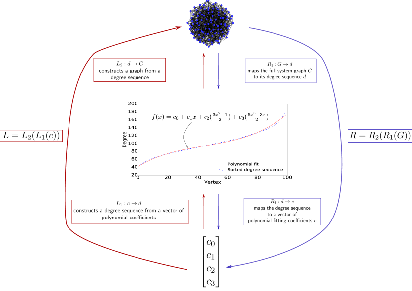
Figure 4: Schematic of our restriction ($\mathbf{R}$) and lifting ($\mathbf{L}$) procedures. The graph’s sorted degree sequence is calculated ($R_{1}$) and then fit to a third-order polynomial ($R_{2}$). This maps graphs ($G$) to vectors of four coefficients ($\mathbf{c}$). To lift, the polynomial is used to generate a degree sequence ($L_{1}$), which is then used to construct a consistent graph ($L_{2}$). This process maps vectors of four coefficients ($\mathbf{c}$) to graphs ($G$). $\mathbf{R}=R_{2}\circ R_{1}$ is our restriction and $\mathbf{L}=L_{2}\circ L_{1}$ is our lifting.

3.2 Restriction

The restriction operator “translates” the full network description to its corresponding coarse variable values. Here, this involves mapping a multigraph to its sorted degree sequence, a simple calculation. However, we may be able to further reduce the dimensionality of our coarse system by keeping not the entire length-$n$ degree sequence, but rather a low-order polynomial fitting of it. To do so, we first sort the sequence to achieve a smooth, monotonically increasing dataset, then fit the result to a third-order polynomial, which had been observed to closely approximate the sequence evolution throughout time. Our coarse description thus consisted, at every moment in time, of the four polynomial coefficient values, specifying a particular sorted degree sequence, as shown in Fig. (4). The restriction operator therefore maps multigraphs to length-four coefficient vectors. This procedure is represented by the blue arrows of Fig. (4).

3.3 Lifting

The lifting operator performs the inverse role of restriction: translating coarse variables into full networks. This is clearly a one-to-many mapping. Specifically in the context of our model, we map vectors of polynomial coefficients to full networks in a two-stage process. First, the coefficient vector is used to recreate a sorted degree sequence by evaluating the full polynomial at integer values and rounding to the nearest degree, as depicted in Fig. (4). If the sum of the resulting degree sequence is odd, a single degree is added to the largest value to ensure the sequence is graphical. Second, this degree sequence is used as input to any algorithm that produces a network consistent with a graphical degree sequence (here we typically used a Havel-Hakimi algorithm, creating a graph whose degree sequence matches that of the input havel_remark_1955 ; hakimi_realizability_1962 ). While the canonical Havel-Hakimi method produces simple graphs, it is not difficult to extend it to multigraphs by allowing the algorithm to wrap around the sequence, producing multiple edges and self-loops. The lifting procedure is represented by the red arrows of Fig. (4).

3.4 Coarse projective integration (CPI)

The components described above are combined to accelerate simulations through Coarse Projective Integration. Denoting the lifting operator by $\mathbf{L}\;:\;c\rightarrow G$ where $c\in\mathbb{R}^{4}$ is the vector of polynomial coefficients, and the restriction operator as $\mathbf{R}\;:G\rightarrow c$, the algorithm progresses as follows:

1. Advance the full system for $t_{h}$ steps

2. Continue for $t_{c}$ steps, restricting the network at intervals and recording the coarse variable values

3. Using the coarse variables collected over the previous $t_{c}$ steps, project each variable forward $t_{p}$ steps with, here, a forward-Euler method

4. With the new, projected coarse variables, lift to one (or more copies of) full network

5. Repeat from Step (1) until the desired time has been reached.

Note that Step (1) is intended to allow a singularly perturbed quantity to approach its slow manifold. Upon initializing a new full system (here, a new network) in Step (4), higher order observables (for example, the triangle count) will be far from the values they would attain in a detailed simulation. If the coarse system model closes with our chosen variables, then either (a) these quantities do not affect the dynamics of the degree sequence; or (b) they do, but then by hypothesis these quantities quickly evolve to functions of the selected coarse variables (i.e., they approach the slow manifold). In the second case, after a short interval of “healing” they will be drawn to the expected trajectory, after which we begin sampling. This is analogous to Fig. (3). The computational gains arise from the projective step, (3). Here, we advance the system $t_{p}$ steps at the cost of one evaluation of forward Euler, instead of $t_{p}$ direct detailed steps.

Results of the application of this general framework with the specific lifting and restriction operators previously outlined are shown in Fig. (5). We used an $n=100$-vertex graph with $m=50000$ edges and parameter value $\kappa=1$. We ran the model for a total of $10\cdot n^{3}$ steps, with $t_{h}=10\cdot n^{2}$, $t_{c}=n^{3}$ and $t_{p}=50\cdot n^{2}$. We see good agreement between the CPI-accelerated and normal systems, while reducing the number of detailed steps by one third. It is important to mention that this method was applied not to a single system instantiation, but to an ensemble of fifty such realizations. This ensured that when properties such as the fitted polynomial coefficients were averaged over the ensemble they evolved smoothly despite the stochastic nature of the system; in effect, we are computing the “expected network evolution” averaged over consistent realizations.

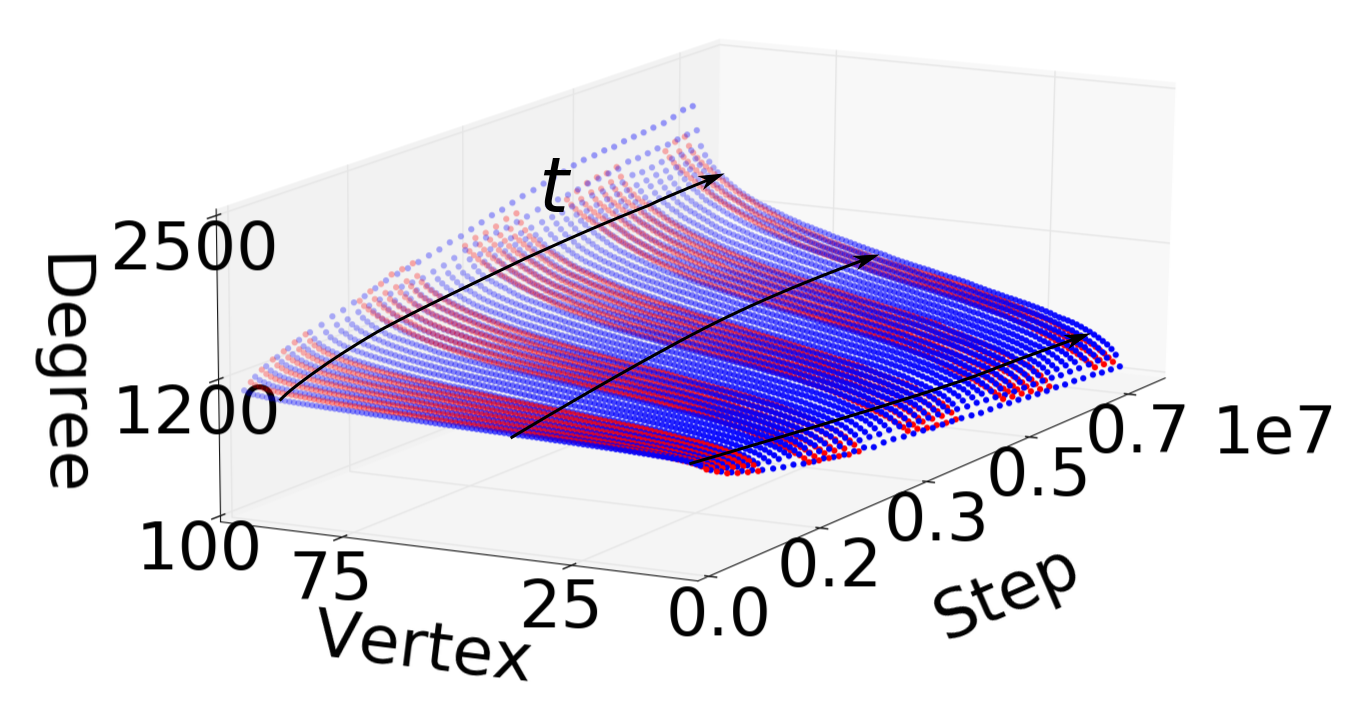
(a)

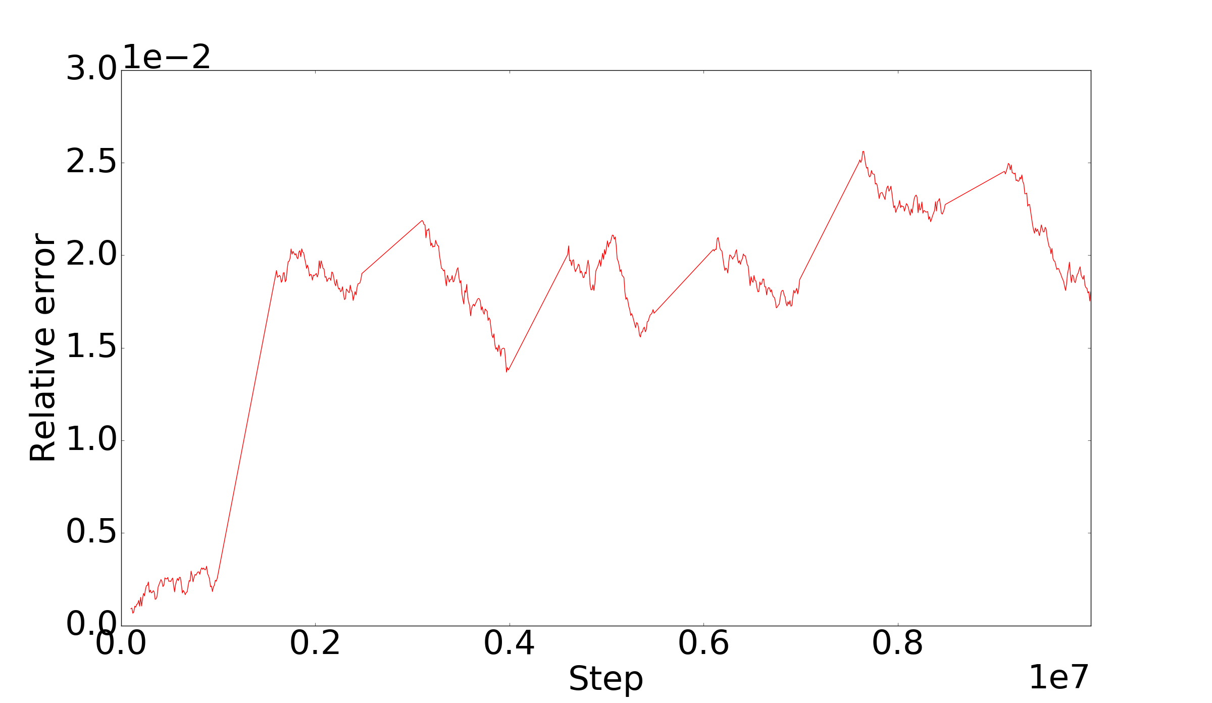
(b)

Figure 5: CPI results: (a) the evolution of the CPI-accelerated degree sequence (red) compared to direct simulation (blue) and (b) error in CPI-accelerated runs calculated by comparing CPI-accelerated degree sequences to those arising from an ensemble of direct simulations.

4 Coarse Newton-GMRES

Aside from the computational savings of model simulations offered by CPI, the equation free framework also permits the calculation of system steady states through fixed point (here, matrix-free Newton-GMRES) algorithms. Referring back to the CPI procedure outlined in Sec. (3.4), we can define an operator $\Theta:\mathbf{d}\rightarrow\mathbf{d}$ projecting coarse variables at $t$ to their values at $t+\delta t$: $\mathbf{d}(t+\delta t)=\Theta(\mathbf{d}(t))$. Note that in this section, we take the sorted degree sequence as our coarse variable. A system fixed point could then be located by employing Newton’s method to solve the equation

$$\mathbf{F}(\mathbf{d})\equiv\Theta(\mathbf{d})-\mathbf{d}=0$$ (1)

However, this requires the repeated solution of the system of linear equations $DF(\mathbf{d}^{(k)})\cdot\delta\mathbf{d}^{(k+1)}=-\mathbf{F}(\mathbf{d}^{(j)})$, in which the system Jacobian, $DF$ is unavailable. Thankfully, we may circumvent this obstacle by estimating the directional derivatives $DF(\mathbf{d})\cdot\delta\mathbf{d}$ via a difference approximation of the form

$$DF(d)\cdot\delta\mathbf{d}\approx\frac{\|\delta\mathbf{d}\|\mathbf{F}(\mathbf{d}+h\|\mathbf{d}\|\frac{\delta\mathbf{d}}{\|\delta\mathbf{d}\|})-\mathbf{F}(\mathbf{d})}{h\|\mathbf{d}\|}$$ (2)

for nonzero $\mathbf{d}$, which in turn is evaluated through calls to $\mathbf{F}$ as defined in Eq. (1)

This is precisely the approach of the Newton-GMRES method, in which the solution to a linear system is sought for in expanding Krylov subspaces kelley_solving_2003 . Applying this algorithm in conjunction with the $\Theta$ operator defined in Sec. (3.4) allowed us to locate the stationary distribution without simply running and observing the full system for long times, as would otherwise be required. Results are shown in Fig. (6). We note that coarse stability results can also be obtained via an iterative Arnoldi eigensolver, again estimating matrix-vector products as above.

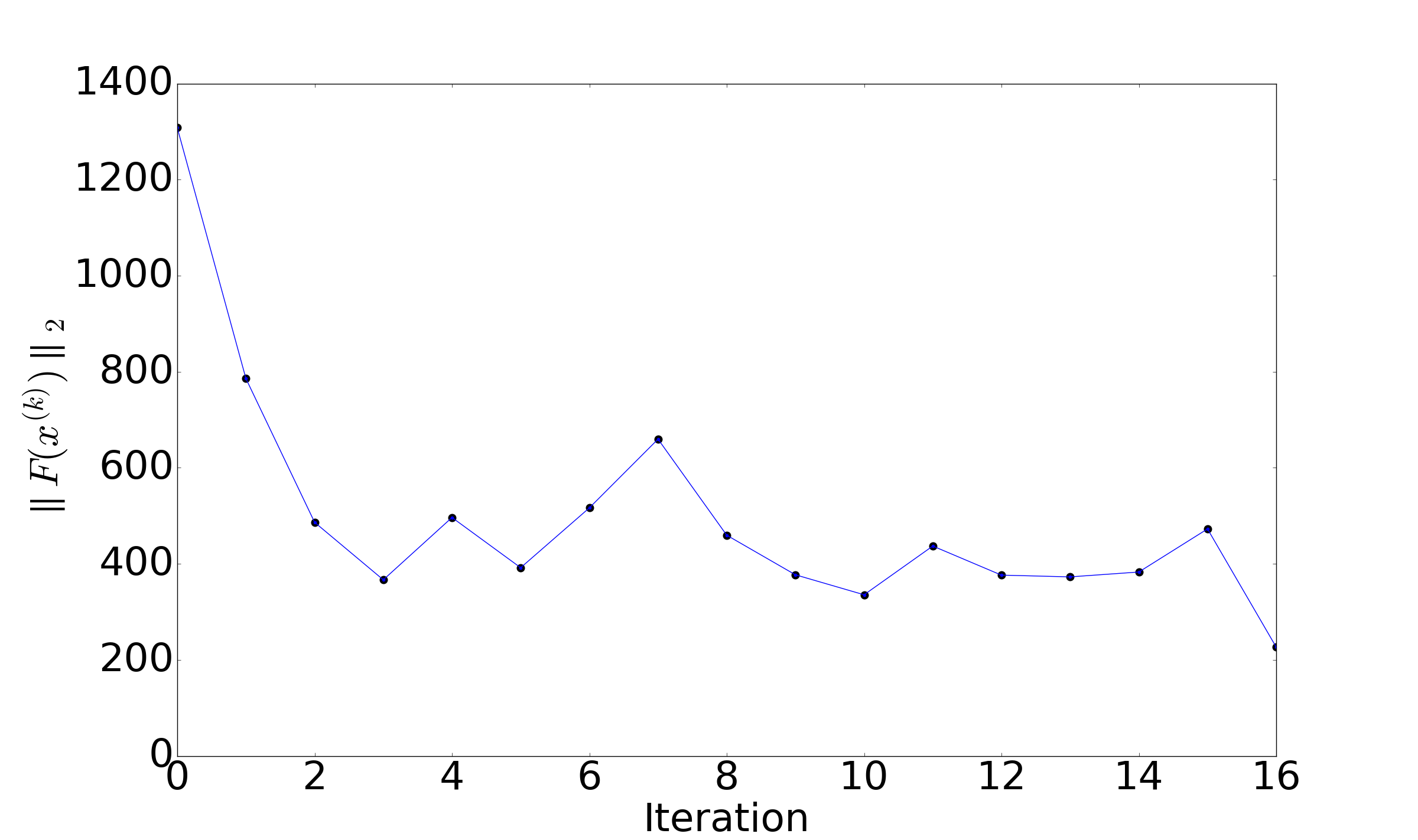
(a)

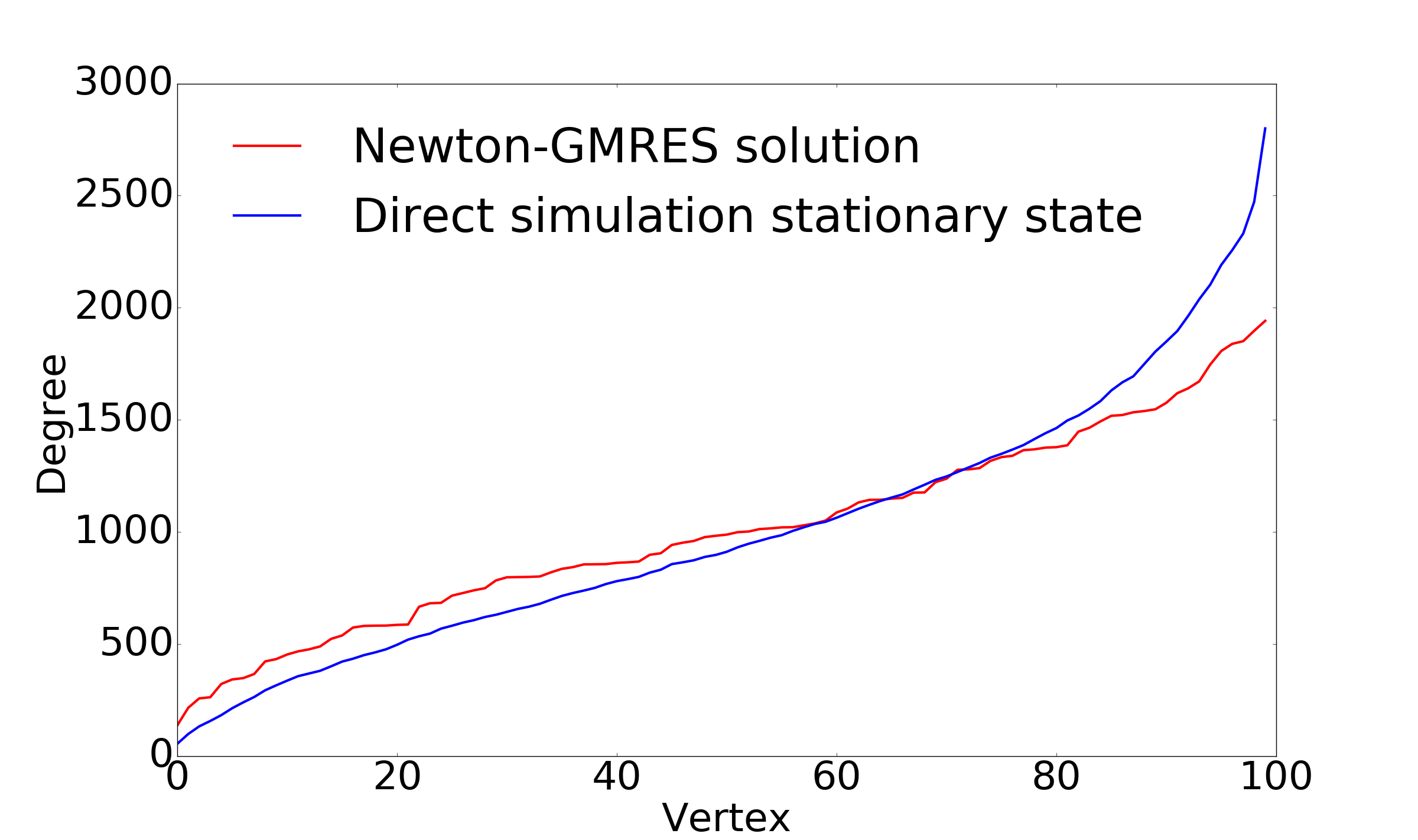
(b)

Figure 6: Coarse Newton-GMRES results: (a) evolution of the error in the coarse Newton-GMRES iteration scheme; and (b) visual comparison of the algorithm’s solution to the stationary state obtained from direct simulation.

5 Algorithmic coarse-graining

Crucial to the above analysis was the determination of suitable coarse, system variables: it is the starting point of any equation free method. However, the discovery of such a low-dimensional description is highly non-trivial. Currently, as in this paper, they are “discovered through informed experience”: through careful investigation of direct simulations, and knowledge of previous analytical results. Clearly, any process which could algorithmically guide this search based on only simulation data would be of great benefit to the modeling practitioner. We now illustrate two such algorithms: principal component analysis (PCA) and diffusion maps (DMAPS). First, we briefly discuss some aspects of the important issue of defining distances between networks, a prerequisite for any dimensionality-reduction technique.

5.1 On network distances

When applying dimensionality reduction techniques to a dataset, it is necessary to define a distance (or similarity) between each pair of data points. If these points are a set of vectors in $\mathbb{R}^{n}$ one has a number of metrics to choose from, the Euclidean distance being a common first option. Unfortunately, when individual points are not vectors but networks, the definition of a useful and computationally easily quantified metric becomes far more challenging. Examples such as the maximal common subgraph and edit distances, defined in bunke_graph_1998 and gao_survey_2010 define metrics on the space of graphs, but their computation is $NP\textnormal{-}hard$. Other computationally feasible approaches include comparing distributions of random walks on each graph vishwanathan_graph_2010 , calculating the so-called $n$-tangle density gallos_revealing_2014 , or calculating the edit distance with an approximation algorithm riesen_approximate_2009 ; zeng_comparing_2009 .

The strategy used in the following computations, detailed in rajendran_analysis_2013 and xiao_structure-based_2008 , enumerates the number of times a certain set of motifs (or subgraphs) appears in each network in the dataset. This maps each network to a vector in $\mathbb{R}^{n}$, and the Euclidean distance is subsequently used to quantify the similarity of two graphs. Due to computational restrictions, we chose here to only count the number of three- and four-vertex single-edge subgraphs contained in each network. As there are eight such motifs, shown in Fig. (7), this process $\gamma$ maps each graph to an eight-dimensional vector: $\gamma:G\rightarrow\mathbb{R}^{8}$. We applied this operation to a simplified version of each graph, wherein any multiple edges were reduced to a single edge.

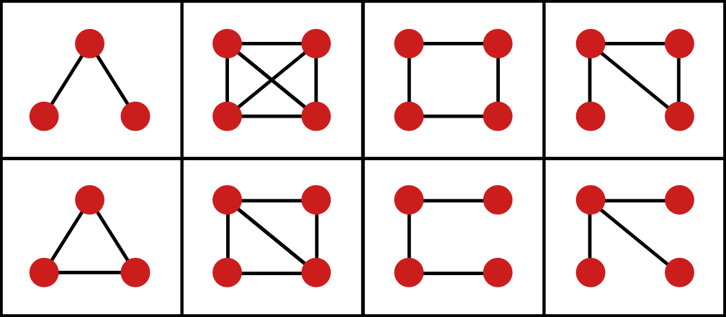
Figure 7: List of the single-edge subgraphs used to embed each network. The number of times each appeared in the simplified input graph was calculated, mapping input graphs to $\mathbb{R}^{8}$.

5.2 PCA

PCA is used to embed data into linear subspaces that capture the directions along which the data varies most jolliffe_principal_2014 . Given some matrix $X\in\mathbb{R}^{n\times m}$ in which each of the $m$ column vectors $x_{i}$ represents a different collection of the $n$ system variables (i.e. a different data point), PCA computes a reduced set of $k<n$, orthogonal “principal components” $z_{i}\in\mathbb{R}^{n}$ that constitute an optimal basis for the data in the sense that, among linear, $k$-dimensional embeddings, $w_{i}=Z^{T}x_{i}$ captures the maximum possible variance in the dataset, where $Z=\begin{bmatrix}|&|&&|\\ z_{1}&z_{2}&\ldots&z_{k}\\ |&|&&|\end{bmatrix}$. This approach has found wide application, but can suffer from its inability to uncover simple nonlinear relationships among the input variables. Indeed, many datasets will not “just lie along some hyperplane” embedded in $\mathbb{R}^{n}$, but will rather lie on a low-dimensional nonlinear manifold throughout the space.

Theoretical results in rath_time_2012 state that, for a given network size $n$, the final stationary state depends only on the number of edges present $m$ and the model parameter $\kappa$. To assess both the validity of our graph embedding technique and the usefulness of PCA in the context of complex networks, we generated a dataset of stationary states over a range of $m\in[50,5000]$ and $\log(\kappa)\in[0,2]$ values by directly running the model over $2n^{3}$ steps ($N=30$ values of each parameter were taken, for a total of $900$ networks). We fixed the network size to $n=50$ vertices. Each resulting graph $G(m_{i},\kappa_{j})=G_{ij}$ was then embedded into $\mathbb{R}^{8}$ by counting the number of times each of the subgraphs shown in Fig. (7) appeared in the network. Thus $\gamma(G_{ij})=v_{ij}\in\mathbb{R}^{8}$. We then proceeded to perform a principal component analysis on this collection of vectors $\{v_{ij}\}_{i,j=1}^{N}$. Interestingly, the first two principal components $z_{1}$ and $z_{2}$ succeeded in uncovering a two-dimensional embedding of the dataset corresponding to the two underlying parameters $m$ and $\kappa$, as shown in Fig. (8) in which the data is projected on the plane spanned by these two vectors. This suggests that, given some final network state $G(m,\kappa)$, by projecting its embedding onto these first two principal components one could obtain a reasonable approximation of the hidden parameter $\kappa$.

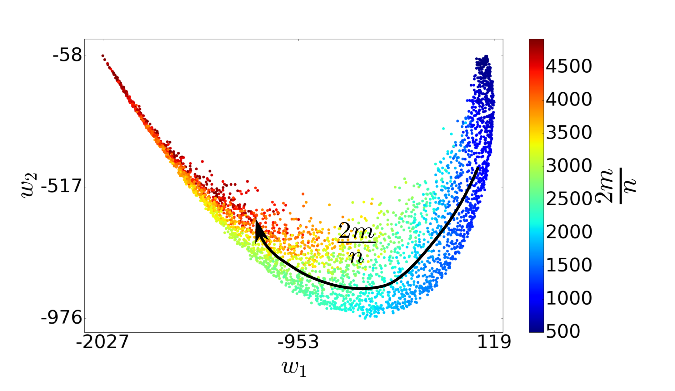
(a)

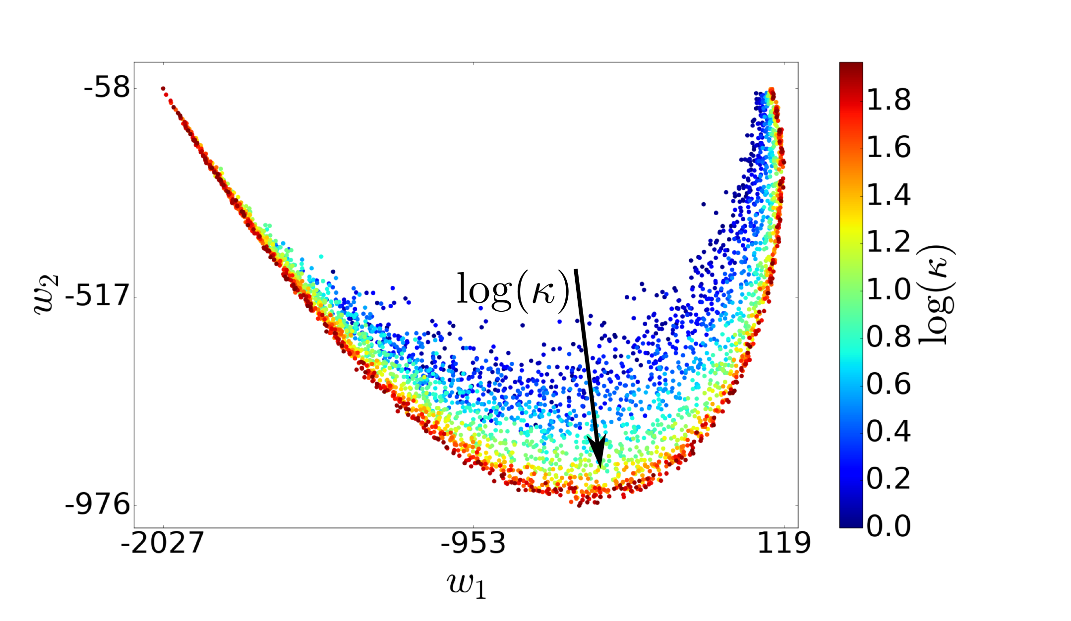
(b)

Figure 8: PCA of motif-based embeddings: (a) coloring the two-dimensional PCA embedding with $\rho$ and (b) coloring the two-dimensional PCA embedding with $\kappa$.

5.3 Diffusion Maps

Unlike PCA, DMAPS uncovers parameterizations of nonlinear manifolds hidden in the data. This is achieved by solving for the discrete equivalent of the eigenfunctions and eigenvalues of the Laplace-Beltrami operator over the manifold, which amounts to calculating leading eigenvector/eigenvalue pairs of a Markov matrix $A$ describing a diffusion process on the dataset. As the eigenfunctions of the Laplace-Beltrami operator provide parameterizations of the underlying domain, the output eigenvectors $\Phi_{i}$ from DMAPS similarly reveal and parameterize any hidden nonlinear structure in the input dataset. The $k$-dimensional DMAP of point $x_{i}$ is given by

$$\Psi(x_{i};t)=\begin{bmatrix}\lambda_{1}^{t}\Phi_{1}(i)\\ \lambda_{2}^{t}\Phi_{2}(i)\\ \vdots\\ \lambda_{k}^{t}\Phi_{k}(i)\end{bmatrix}$$

where $\lambda_{i}$ is the $i^{th}$ eigenvalue of the Markov matrix $A$, $\Phi_{i}(j)$ the $j^{th}$ entry of eigenvector $i$, and the parameter $t$ allows one to probe multiscale features in the dataset. See coifman_diffusion_2006 ; nadler_diffusion_2006 for further details.

First we applied DMAPS to the dataset described in Sec. (5.2). Given the apparent success of PCA in this setting, one would expect DMAPS to also uncover the two-dimensional embedding corresponding to different values of $m$ and $\kappa$. Fig. (9) shows that this is indeed the case: using $\Phi_{1}$ and $\Phi_{4}$ to embed the graphs produces a two-dimensional surface along which both $\rho$ and $\kappa$ vary independently.

Additionally, we were interested in embeddings of different model trajectories. This dataset was generated by sampling two different model simulations as they evolved ($N=2000$ points were sampled from each trajectory). The parameters $n$, $m$ and $\kappa$ were held constant at $200$, $20100$ and $1.0$ respectively, but one graph was initialized as an Erdős-Rényi random graph (Fig. (2(b))), while the other was initialized as a “lopsided” graph (Fig. (2(a))). Every $500$ steps the graph would be recorded till $N$ snapshots were taken of each trajectory, for a total of $1000000$ steps. Letting $G_{e}(t)$ refer to the Erdős-Rényi-initialized system at step $t$, and $G_{l}(t)$ the lopsided-initialized system, the embedding $\gamma$ was used to create points $\gamma(G_{e}(t))=v_{e}(t)\in\mathbb{R}^{8}$ and similarly $\gamma(G_{l}(t))=v_{l}(t)\in\mathbb{R}^{8}$.

DMAPS was then applied to this set of $2N$ points, and the three-dimensional embedding using $\Phi_{1}$, $\Phi_{2}$ and $\Phi_{3}$ is shown in Fig. (10). At first, the two trajectories are mapped to distant regions in $\mathbb{R}^{3}$ due to their different initial conditions. They evolve along different “regions” of the embedding, taking two distinct trajectories on their approach to the stationary state. Eventually, their embeddings meet as they arrive at this final, shared state, each asymptotically along opposite sides of the slowest eigenvector of the linearization of the steady state. DMAPS thus proves useful in elucidating both geometric and dynamic features of the system as shown in Figs. (9) and (10).

We see that both PCA and DMAPS, when combined with a suitable embedding of each graph, can help uncover useful information pertaining to the underlying dimensionality of the problem dynamics.

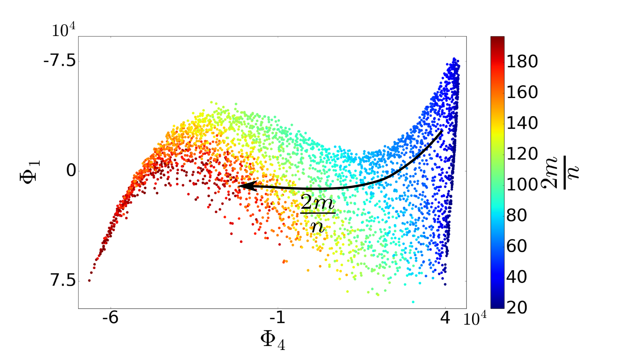
(a)

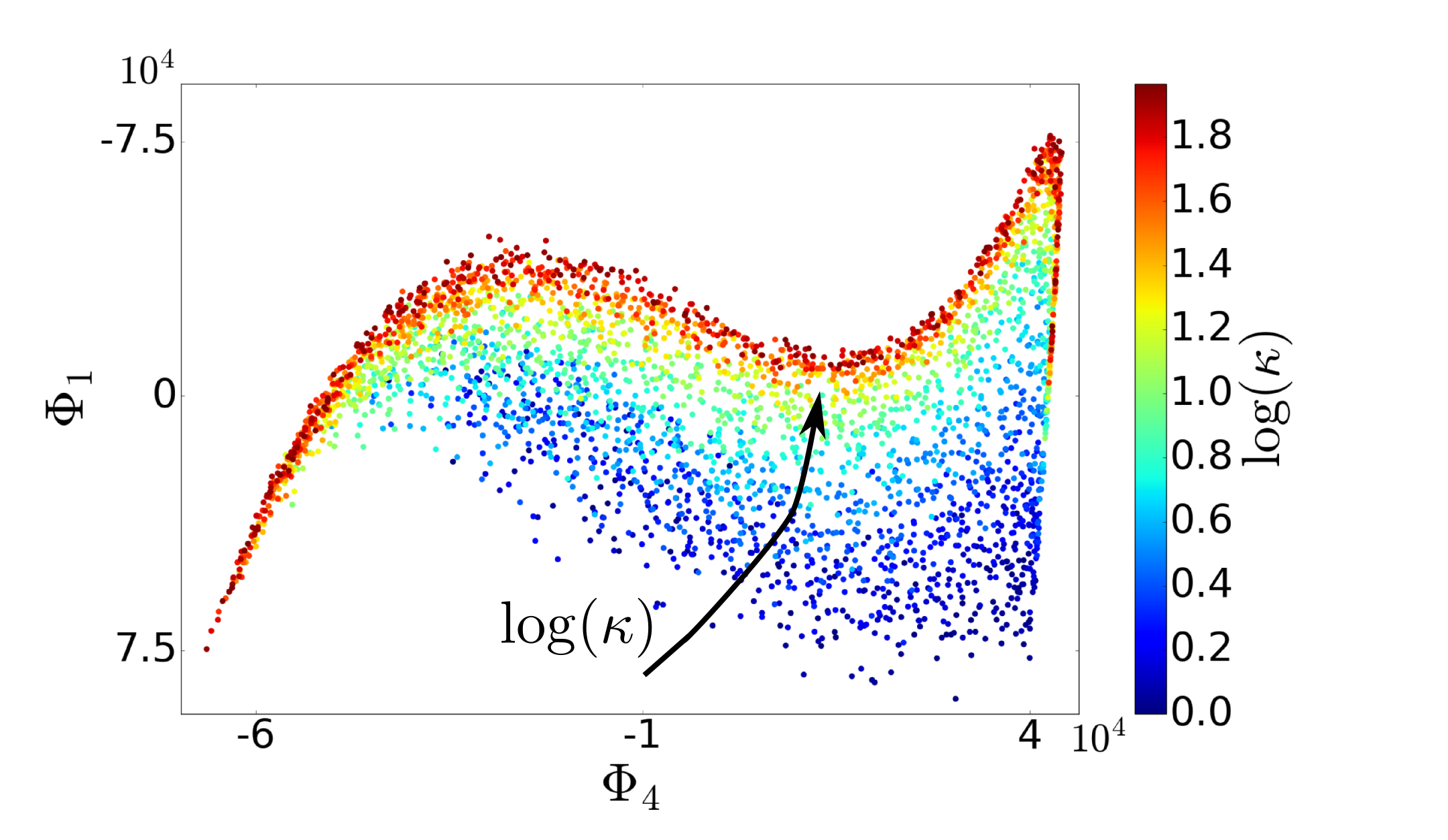
(b)

Figure 9: DMAP of motif-based embeddings from a collection of simulations run at different parameter values: (a) coloring the two-dimensional DMAPS embedding with $\rho$ and (b) coloring the two-dimensional DMAPS embedding with $\kappa$. As with PCA, DMAPS uncovered the parameters governing the stationary state, known from rath_time_2012

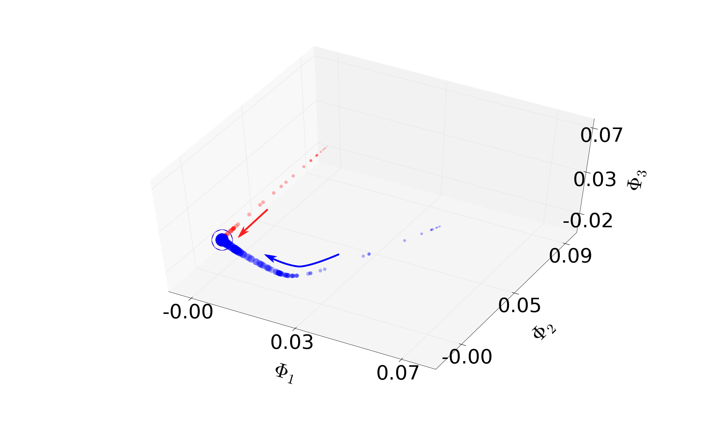
(a)

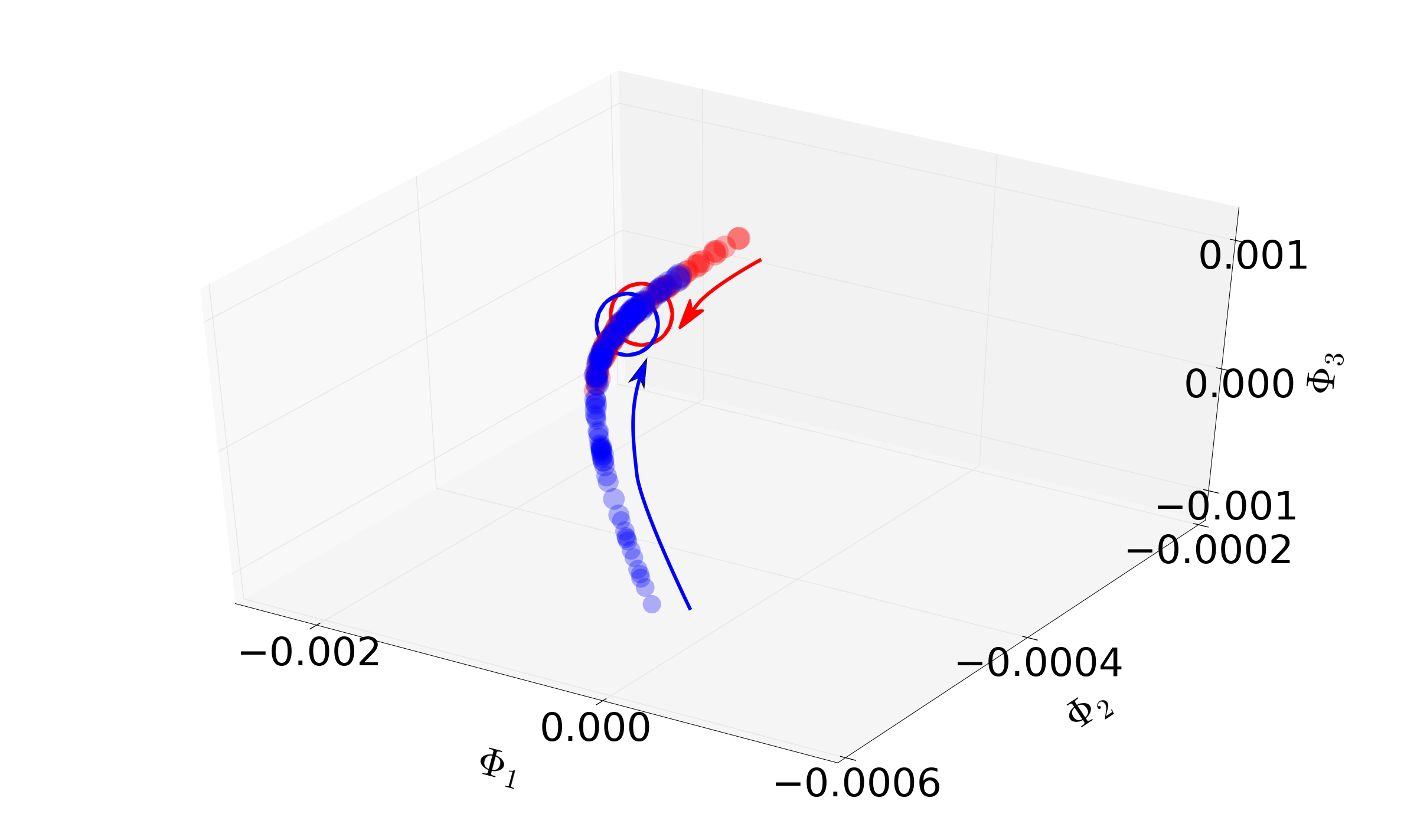
(b)

Figure 10: DMAP of motif-based embeddings from two separate simulation trajectories: (a) embedding of two trajectories starting from different initial conditions. While the trajectories are initially mapped to separate regions of “embedding space”, they eventually evolve to the same coarse stationary state. Final states are circled, and point size grows as more steps are taken in each trajectory. (b) Enlarged view of the final points in the previous plot, revealing the approach to a similar final state along opposite sides of the slowest eigenvector of its linearization. Here, the average of the final fifty points is circled. Due to the stochastic nature of the system, the final embeddings mildly fluctuate randomly about the shared stationary state.

6 Conclusion

The equation free framework was successfully applied to the edge-conservative preferential attachment model, accelerating simulations through CPI and locating stationary states through coarse Newton-GMRES. This indicates potential avenues for improving simulation times of other complex network models, such as those found in epidemiology. Additionally, an underlying two-dimensional description was uncovered via PCA and DMAPS. These automated methods of dimensionality-reduction are quite general, and can in principle be applied in a wide range of network settings to probe hidden low-dimensional structure. For an application in the setting of labeled nodes, see (kattis_modeling_2016 ).

However, an open area of investigation is the interpretation of the output from the PCA and DMAPS techniques. As a linear map, PCA retains a clear relationship between its input and output, but is less effective when data lie on highly nonlinear manifolds. DMAPS may perform better the task of dimensionality reduction, but it is unclear how the embedding coordinates relate to physical features of the sampled networks. While this approach opens several promising avenues in coarse-graining complex network dynamics, it also reveals two “bottlenecks” for the process: (a) the selection of informative and practically computable graph distance metrics, necessary in the discovery of good coarse variables; and (b) the construction of network realizations consistent with (conditioned on) specific values of collective observables. Both items are, and we expect will continue being, the subject of intense investigation by many research groups, including ours.

- [1] K. A. Bold, K. Rajendran, B. Ráth, and I. G. Kevrekidis. An equation-free approach to coarse-graining the dynamics of networks. Journal of Computational Dynamics, 1(1):111–134, Apr. 2014.
- [2] D. Brown, J. Feng, and S. Feerick. Variability of Firing of Hodgkin-Huxley and FitzHugh-Nagumo Neurons with Stochastic Synaptic Input. Physical Review Letters, 82(23):4731–4734, June 1999.
- [3] H. Bunke and K. Shearer. A Graph Distance Metric Based on the Maximal Common Subgraph. Pattern Recogn. Lett., 19(3-4):255–259, Mar. 1998.
- [4] R. R. Coifman and S. Lafon. Diffusion maps. Applied and Computational Harmonic Analysis, 21(1):5–30, July 2006.
- [5] R. Durrett, J. P. Gleeson, A. L. Lloyd, P. J. Mucha, F. Shi, D. Sivakoff, J. E. S. Socolar, and C. Varghese. Graph fission in an evolving voter model. Proceedings of the National Academy of Sciences, 109(10):3682–3687, Mar. 2012.
- [6] L. K. Gallos and N. H. Fefferman. Revealing effective classifiers through network comparison. EPL (Europhysics Letters), 108(3):38001, Nov. 2014.
- [7] X. Gao, B. Xiao, D. Tao, and X. Li. A Survey of Graph Edit Distance. Pattern Anal. Appl., 13(1):113–129, Jan. 2010.
- [8] C. W. Gear, J. M. Hyman, P. G. Kevrekidid, I. G. Kevrekidis, O. Runborg, and C. Theodoropoulos. Equation-Free, Coarse-Grained Multiscale Computation: Enabling Mocroscopic Simulators to Perform System-Level Analysis. Communications in Mathematical Sciences, 1(4):715–762, 2003.
- [9] S. L. Hakimi. On Realizability of a Set of Integers as Degrees of the Vertices of a Linear Graph. I. Journal of the Society for Industrial and Applied Mathematics, 10(3):496–506, 1962.
- [10] V. Havel. A Remark on the Existence of Finite Graphs (Czech). Časopis pro pěstování matematiky, 80(4):477–480, 1955.
- [11] A. M. Hermundstad, K. S. Brown, D. S. Bassett, and J. M. Carlson. Learning, memory, and the role of neural network architecture. PLoS computational biology, 7(6):e1002063, June 2011.
- [12] A. L. Hodgkin and A. F. Huxley. A quantitative description of membrane current and its application to conduction and excitation in nerve. The Journal of Physiology, 117(4):500–544, Aug. 1952.
- [13] I. Jolliffe. Principal Component Analysis. In Wiley StatsRef: Statistics Reference Online. John Wiley & Sons, Ltd, 2014.
- [14] J. Joubert, P. Fourie, and K. Axhausen. Large-Scale Agent-Based Combined Traffic Simulation of Private Cars and Commercial Vehicles. Transportation Research Record: Journal of the Transportation Research Board, 2168:24–32, Nov. 2010.
- [15] A. A. Kattis, A. Holiday, A.-A. Stoica, and I. G. Kevrekidis. Modeling epidemics on adaptively evolving networks: A data-mining perspective. Virulence, 7(2):153–162, Feb. 2016.
- [16] C. T. Kelley. Solving Nonlinear Equations with Newton’s Method. SIAM, Jan. 2003.
- [17] I. G. Kevrekidis, C. W. Gear, and G. Hummer. Equation-free: The computer-aided analysis of complex multiscale systems. AIChE Journal, 50(7):1346–1355, July 2004.
- [18] B. Nadler, S. Lafon, R. R. Coifman, and I. G. Kevrekidis. Diffusion maps, spectral clustering and reaction coordinates of dynamical systems. Applied and Computational Harmonic Analysis, 21(1):113–127, July 2006.
- [19] K. Rajendran and I. G. Kevrekidis. Coarse graining the dynamics of heterogeneous oscillators in networks with spectral gaps. Physical Review E, 84(3):036708, Sept. 2011.
- [20] K. Rajendran and I. G. Kevrekidis. Analysis of data in the form of graphs. arXiv:1306.3524 [physics], June 2013. arXiv: 1306.3524.
- [21] K. Riesen and H. Bunke. Approximate graph edit distance computation by means of bipartite graph matching. Image and Vision Computing, 27(7):950–959, June 2009.
- [22] B. Roche, J. M. Drake, and P. Rohani. An agent-based model to study the epidemiological and evolutionary dynamics of Influenza viruses. BMC bioinformatics, 12:87, 2011.
- [23] B. Ráth. Time evolution of dense multigraph limits under edge-conservative preferential attachment dynamics. Random Structures & Algorithms, 41(3):365–390, Oct. 2012.
- [24] B. Ráth and L. Szakács. Multigraph limit of the dense configuration model and the preferential attachment graph. Acta Mathematica Hungarica, 136(3):196–221, Apr. 2012.
- [25] C. I. Siettos. Equation-Free multiscale computational analysis of individual-based epidemic dynamics on networks. Applied Mathematics and Computation, 218(2):324–336, Sept. 2011.
- [26] J. M. Swaminathan, S. F. Smith, and N. M. Sadeh. Modeling Supply Chain Dynamics: A Multiagent Approach*. Decision Sciences, 29(3):607–632, July 1998.
- [27] S. V. N. Vishwanathan, N. N. Schraudolph, R. Kondor, and K. M. Borgwardt. Graph Kernels. Journal of Machine Learning Research, 11:1201−1242, Apr. 2010.
- [28] Y. Xiao, H. Dong, W. Wu, M. Xiong, W. Wang, and B. Shi. Structure-based graph distance measures of high degree of precision. Pattern Recognition, 41(12):3547–3561, Dec. 2008.
- [29] Z. Zeng, A. K. H. Tung, J. Wang, J. Feng, and L. Zhou. Comparing Stars: On Approximating Graph Edit Distance. Proc. VLDB Endow., 2(1):25–36, Aug. 2009.