Network-Wide Distributed Carrier Frequency Offsets Estimation and Compensation

Jian Du and Yik-Chung Wu The authors are with the Department of Electrical and Electronic Engineering, The University of Hong Kong, Pokfulam Road, Hong Kong (e-mail: dujianeee@gmail.com, ycwu@eee.hku.hk).
Abstract

In this paper, we propose a fully distributed algorithm for frequency offsets estimation in decentralized systems. With the proposed algorithm, each node estimates its frequency offsets by local computations and limited exchange of information with its direct neighbors. Such algorithm does not require any centralized information processing or knowledge of global network topology. It is shown analytically that the proposed algorithm always converges to the optimal estimates regardless of network topology. Simulation results demonstrate the fast convergence of the algorithm and show that estimation mean-squared-error at each node touches the centralized Cramér-Rao bound within a few iterations of message exchange. Therefore, the proposed method has low overhead and is scalable with network size.

Index Terms:
Carrier frequency offsets (CFOs) estimation, heterogeneous networks, factor graph, convergence analyses.

I Introduction

In wireless communication systems, local oscillators are used in transceivers to generate carrier signals required for up-conversion and down-conversion. Ideally, carrier frequencies produced by oscillators of each transceiver pair should be the same. However, in practice, frequencies synthesized from independent oscillators will be different from each other due to variation of oscillator circuits. The received signal impaired by carrier frequency offsets (CFOs) between transmitter and receiver leads to a continuous rotation of symbol constellation, resulting in degradation of system capacity and bit error rate (BER) [1, 2, 3, 4]. Consequently, carrier frequency synchronization has always been a momentous issue in communication systems.

As modern wireless environments become more heterogeneous and decentralized, mobile terminals in a network engage more and more cooperative communications and distributed computations [5], new scenarios that require multiple wireless units to synchronize with each other arise. For example,

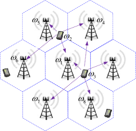
Distributed beamforming: As shown in Fig. 1(a), to improve the range of communications and save battery power during the transmission, multiple mobile terminals form a virtual antenna array and cooperatively direct a beam in the desired direction of transmission [6], [7]. Since each source node in the distributed beamformer has an independent local oscillator, common carrier frequency among all transmitters is crucial to ensure that a beam is aimed in the desired direction.

Multi-cell cooperation: In fully frequency reuse cellular systems as depicted in Fig. 1(b), despite different users interfere with each other, multiple base stations could coordinate their coding and decoding. It was shown that such joint-processing significantly outperforms a network with individual cell processing [8, 9]. Yet, multiple base-stations cooperation requires frequency synchronization so that there is no CFO between each pair of communication link [10].

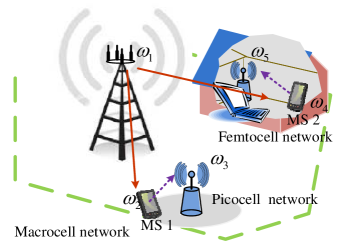
Heterogenous Networks (HetNets): HetNets have attracted much attention from both industry and academia in the past few years. As shown in Fig. 1(c), in a 3-tier HetNet, a mobile may wish to be associated with different tier base stations in the uplink and downlink to obtain optimal performance [11, 12, 13]. However, multi-tier cooperation is possible only when different tiers of networks are frequency-synchronized to each other.

The above examples of network-wide synchronization problem can be summarized and reduced to a multi-node communication systems as shown in Fig. 2. Despite relative CFO between each pair of nodes can be optimally estimated by existing methods [14, 21, 19, 18, 17, 16, 20, 15, 22, 23], network-wide CFOs correction is difficult since each node needs to synchronize with multiple neighboring nodes with different relative CFOs at the same time. Making the problem more challenging is the fact that synchronization should be accomplished by local operations without knowing the global network structure since users move around and join different parts of the network randomly.

Pioneering works for network CFOs correction have been proposed in [24],[25]. By gathering all the information in a central processing unit, CFOs are estimated at the receiver and then fedback to corresponding transmitters to adjust the offsets. These methods are centralized, which are not suitable for large-scale network. On the other hand, [26, 27, 28] investigated methods for frequency synchronization in distributed beamforming systems. However, these methods require the formation and maintenance of special network structures (e.g., tree structure in [26], ring structure in [27] and chain structure in [28]), thus suffer from large overhead and long delay, and are not scalable with network size. Recently, [29] proposed the distributed frequency-locked loops (D-FLL) to control and synchronize the carrier frequencies of autonomous nodes based on average consensus principle. Notwithstanding the distributed carrier frequency calibration advantage, fully distributed D-FLL approach suffers from very slow convergence rate as shown in [29]. Furthermore, the D-FLL algorithm is designed exclusively for single path channel. Even in a simple point-to-point case with multi-path channel, the D-FLL cannot be applied directly.

In this paper, we propose a network-wide fully distributed CFOs estimation and compensation method which only involves local processing and information exchange between neighboring nodes. There is no need to have a central hub that aggregates information and no knowledge about the global network topology is required. The frequency offset of each oscillator is estimated and corrected locally in each node. After synchronization, there is no frequency offset between any pair of nodes in the network. The proposed algorithm is scalable with network size, and robust to topology changes. The convergence of the proposed method is also formally proved.

The rest of this paper is organized as follows. System model is presented in Section II. Fully distributed frequency offsets estimation and correction based on belief propagation (BP) is derived in Section III . The convergence property of the proposed method is analyzed in Section IV. Simulation results are given in Section IV and, finally, conclusions are provided in Section V.

Notations: Boldface uppercase and lowercase letters will be used for matrices and vectors, respectively. 𝔼𝔼\mathbb{E} denotes the expectation over the random variables. Superscripts H𝐻H and T𝑇T denote Hermitian and transpose, respectively. The symbol 𝑰Nsubscript𝑰𝑁\bm{I}_{N} represents the N×N𝑁𝑁N\times N identity matrix, while 𝟏Ksubscript1𝐾\bm{1}_{K} is an all one K𝐾K dimensional vector. The symbol tensor-product\otimes denotes the Kronecker product and direct-product\odot denotes the Hadamard product. Notation 𝒩(𝒙|𝝁,𝑹)𝒩conditional𝒙𝝁𝑹{\mathcal{N}}(\bm{x}|\bm{\mu},\bm{R}) stands for the probability density function (pdf) of a Gaussian random vector 𝒙𝒙\bm{x} with mean 𝝁𝝁\bm{\mu} and covariance matrix 𝑹𝑹\bm{R}. The symbol proportional-to\propto represents the linear scalar relationship between two real valued functions. diag{[a1,,aN]}diagsubscript𝑎1subscript𝑎𝑁\mathrm{diag}\{[a_{1},\ldots,a_{N}]\} corresponds to an N×N𝑁𝑁N\times N diagonal matrix with diagonal components a1subscript𝑎1a_{1} through aNsubscript𝑎𝑁a_{N}, while blkdiag{[𝑨1,,𝑨N]}blkdiagsubscript𝑨1subscript𝑨𝑁\mathrm{blkdiag}\{[\bm{A}_{1},\ldots,\bm{A}_{N}]\} corresponds to a block diagonal matrix with 𝑨1subscript𝑨1\bm{A}_{1} through 𝑨Nsubscript𝑨𝑁\bm{A}_{N} as diagonal blocks. For two matrices 𝑿𝑿\bm{X} and 𝒀𝒀\bm{Y}, 𝑿𝒀succeeds-or-equals𝑿𝒀\bm{X}\succeq\bm{Y} means that 𝑿𝒀𝑿𝒀\bm{X}-\bm{Y} is a positive semi-definite matrix.

II System Model

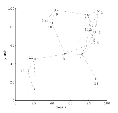
We consider a network consisting of K𝐾K nodes distributed in a field as shown in Fig. 2. The topology of the network is described by a communication graph 𝒢=(𝒱,)𝒢𝒱\mathcal{G}=(\mathcal{V},\mathcal{E}) of order K𝐾K, where 𝒱={1,,K}𝒱1𝐾\mathcal{V}=\{1,\ldots,K\} is the set of graph vertexes, and 𝒱×𝒱𝒱𝒱\mathcal{E}\subseteq\mathcal{V}\times\mathcal{V} is the set of graph edges. In the example shown in Fig. 2, the vertices are depicted by circles and the edges by lines connecting these circles. The neighborhood of node i𝑖i is the set of nodes (i)𝒱𝑖𝒱\mathcal{I}(i)\subset\mathcal{V} defined as (i){j𝒱|{i,j}}𝑖conditional-set𝑗𝒱𝑖𝑗\mathcal{I}(i)\triangleq\{j\in\mathcal{V}|\{i,j\}\in\mathcal{E}\}, i.e., those nodes that are connected via a direct communication link to node i𝑖i. It is also assumed that any two distinct nodes can communicate with each other through finite hops, such graph is named strongly connected graph.

In general, relative CFOs exist between any pair of neighboring nodes, and can be estimated by traditional CFOs estimation methods. Let nodes i𝑖i and j𝑗j equipped with Nisubscript𝑁𝑖N_{i} and Njsubscript𝑁𝑗N_{j} antennas, respectively. Denote the frequency offsets (with respect to a reference frequency) of the qthsuperscript𝑞𝑡q^{th} antenna on node i𝑖i as ωqisubscriptsuperscript𝜔𝑖𝑞\omega^{i}_{q}, while that of kthsuperscript𝑘𝑡k^{th} antenna of node j𝑗j as ωkjsubscriptsuperscript𝜔𝑗𝑘\omega^{j}_{k}. Then, the relative CFO between the qthsuperscript𝑞𝑡q^{th} and kthsuperscript𝑘𝑡k^{th} antenna of node i𝑖i and j𝑗j respectively is ϵq,ki,jωqiωkjsubscriptsuperscriptitalic-ϵ𝑖𝑗𝑞𝑘subscriptsuperscript𝜔𝑖𝑞subscriptsuperscript𝜔𝑗𝑘\epsilon^{i,j}_{q,k}\triangleq\omega^{i}_{q}-\omega^{j}_{k}. Here we consider the general case where each antenna can be associated with separate oscillator circuit. Therefore, for the Multiple Input Multiple Output (MIMO) system between node i𝑖i and node j𝑗j, there are NiNjsubscript𝑁𝑖subscript𝑁𝑗N_{i}N_{j} relative CFOs denoted as ϵi,j[ϵ1,1i,j,,ϵNi,1i,j,,ϵ1,Nji,j,,ϵNi,Nji,j]Tsuperscriptbold-italic-ϵ𝑖𝑗superscriptsubscriptsuperscriptitalic-ϵ𝑖𝑗11subscriptsuperscriptitalic-ϵ𝑖𝑗subscript𝑁𝑖1subscriptsuperscriptitalic-ϵ𝑖𝑗1subscript𝑁𝑗subscriptsuperscriptitalic-ϵ𝑖𝑗subscript𝑁𝑖subscript𝑁𝑗𝑇\bm{\epsilon}^{i,j}\triangleq[\epsilon^{i,j}_{1,1},\dots,\epsilon^{i,j}_{N_{i},1},\ldots,\epsilon^{i,j}_{1,N_{j}},\dots,\epsilon^{i,j}_{N_{i},N_{j}}]^{T}. Such relative CFOs estimation in MIMO systems can be decomposed into Njsubscript𝑁𝑗N_{j} parallel Multiple Input Single Output (MISO) CFOs estimation problem [17]. For example, considering a flat-fading MISO system, for the kthsuperscript𝑘𝑡k^{th} receive antenna of node j𝑗j, the received signal can be written as

yki,j(t)=q=1Nihq,ki,jeȷεq,ki,jtzqi(t)+ξkj(t)t=1,,N,formulae-sequencesubscriptsuperscript𝑦𝑖𝑗𝑘𝑡superscriptsubscript𝑞1subscript𝑁𝑖subscriptsuperscript𝑖𝑗𝑞𝑘superscript𝑒italic-ȷsubscriptsuperscript𝜀𝑖𝑗𝑞𝑘𝑡subscriptsuperscript𝑧𝑖𝑞𝑡subscriptsuperscript𝜉𝑗𝑘𝑡𝑡1𝑁y^{i,j}_{k}(t)=\sum_{q=1}^{N_{i}}h^{i,j}_{q,k}e^{\jmath\varepsilon^{i,j}_{q,k}t}z^{i}_{q}(t)+\xi^{j}_{k}(t)\quad t=1,\ldots,N, (1)

where hq,ki,jsubscriptsuperscript𝑖𝑗𝑞𝑘h^{i,j}_{q,k} are the unknown channel gains between the qthsuperscript𝑞𝑡q^{th} antenna of node i𝑖i and kthsuperscript𝑘𝑡k^{th} antenna of node j𝑗j; ȷ1italic-ȷ1\jmath\triangleq\sqrt{-1}; {zqi(t)}t=1Nsubscriptsuperscriptsubscriptsuperscript𝑧𝑖𝑞𝑡𝑁𝑡1\{z^{i}_{q}(t)\}^{N}_{t=1} is the training sequence transmitted from the qthsuperscript𝑞𝑡q^{th} antennas of node i𝑖i; and ξkj(t)superscriptsubscript𝜉𝑘𝑗𝑡\xi_{k}^{j}(t) is the observation noise at the kthsuperscript𝑘𝑡k^{th} antenna of node j𝑗j. By stacking (1) with t=1,,N𝑡1𝑁t=1,\ldots,N in vector form and omitting superscript i,j𝑖𝑗i,j without confusion, the received vector 𝒚k[yk(1),,yk(N)]Tsubscript𝒚𝑘superscriptsubscript𝑦𝑘1subscript𝑦𝑘𝑁𝑇\bm{y}_{k}\triangleq[y_{k}(1),\ldots,y_{k}(N)]^{T} can be written as

𝒚k=𝜞k(ϵk)𝒁k𝒉k+𝝃kk=1,,Nj,formulae-sequencesubscript𝒚𝑘direct-productsubscript𝜞𝑘subscriptbold-italic-ϵ𝑘subscript𝒁𝑘subscript𝒉𝑘subscript𝝃𝑘𝑘1subscript𝑁𝑗\bm{y}_{k}={\bm{\mathit{\Gamma}}}_{k}(\bm{\epsilon}_{k})\odot\bm{Z}_{k}\bm{h}_{k}+\bm{\xi}_{k}\quad k=1,\ldots,N_{j}, (2)

where 𝜞k(ϵk)subscript𝜞𝑘subscriptbold-italic-ϵ𝑘{\bm{\mathit{\Gamma}}}_{k}(\bm{\epsilon}_{k}) is an N𝑁N-by-Nisubscript𝑁𝑖N_{i} Vandermonde matrix with its tthsuperscript𝑡𝑡t^{th} row given by [eȷtϵ1,k,eȷtϵ2,k,,eȷtϵNi,k]superscript𝑒italic-ȷ𝑡subscriptitalic-ϵ1𝑘superscript𝑒italic-ȷ𝑡subscriptitalic-ϵ2𝑘superscript𝑒italic-ȷ𝑡subscriptitalic-ϵsubscript𝑁𝑖𝑘[e^{\jmath t\epsilon_{1,k}},e^{\jmath t\epsilon_{2,k}},\cdots,e^{\jmath t\epsilon_{N_{i},k}}]; 𝒁ksubscript𝒁𝑘\bm{Z}_{k} is the N𝑁N-by-Nisubscript𝑁𝑖N_{i} training sequence matrix with its tthsuperscript𝑡𝑡t^{th} row [z1(t),z2(t),,zNi(t)]subscript𝑧1𝑡subscript𝑧2𝑡subscript𝑧subscript𝑁𝑖𝑡[z_{1}(t),z_{2}(t),\cdots,z_{N_{i}}(t)]; and 𝝃k=[ξk(1),,ξk(N)]Tsubscript𝝃𝑘superscriptsubscript𝜉𝑘1subscript𝜉𝑘𝑁𝑇\bm{\xi}_{k}=[\xi_{k}(1),\ldots,\xi_{k}(N)]^{T} is the observation noise. The parameters ϵk[ϵ1,k,ϵ2,k,,ϵNi,k]Tsubscriptbold-italic-ϵ𝑘superscriptsubscriptitalic-ϵ1𝑘subscriptitalic-ϵ2𝑘subscriptitalic-ϵsubscript𝑁𝑖𝑘𝑇\bm{\epsilon}_{k}\triangleq[\epsilon_{1,k},\epsilon_{2,k},\dots,\epsilon_{N_{i},k}]^{T} and 𝒉k[h1,k,,hNi,k]Tsubscript𝒉𝑘superscriptsubscript1𝑘subscriptsubscript𝑁𝑖𝑘𝑇\bm{h}_{k}\triangleq[h_{1,k},\dots,h_{N_{i},k}]^{T} are the parameters need to be estimated.

If the noise is white and Gaussian, i.e., 𝝃k𝒞𝒩(𝝃k;𝟎,σk2𝑰N)similar-tosubscript𝝃𝑘𝒞𝒩subscript𝝃𝑘0subscriptsuperscript𝜎2𝑘subscript𝑰𝑁\bm{\xi}_{k}\sim\mathcal{CN}(\bm{\xi}_{k};\bm{0},\sigma^{2}_{k}\bm{I}_{N}), joint relative CFOs and channels estimation have been extensively studied in the past two decades and the optimal estimates ϵ^ksubscript^bold-italic-ϵ𝑘{\hat{\bm{\epsilon}}}_{k} and 𝒉^ksubscript^𝒉𝑘\hat{\bm{h}}_{k} have been proposed in[16, 17, 18, 19, 20], with the mean-square-errors (MSEs) approaching the corresponding Cramér-Rao bounds (CRBs) in medium and high signal-to-noise ratio (SNR) ranges. From (2), the CRB of ϵksubscriptbold-italic-ϵ𝑘{\bm{\epsilon}}_{k} can be shown to be [17]

𝑩ϵk(ϵk,𝒉k)=σk22{Re[𝑽k𝑻kH(𝜦kH𝜦k)1𝑻k]}1,subscript𝑩subscriptbold-italic-ϵ𝑘subscriptbold-italic-ϵ𝑘subscript𝒉𝑘superscriptsubscript𝜎𝑘22superscriptRedelimited-[]subscript𝑽𝑘superscriptsubscript𝑻𝑘𝐻superscriptsubscriptsuperscript𝜦𝐻𝑘subscript𝜦𝑘1subscript𝑻𝑘1\bm{B}_{{\bm{\epsilon}}_{k}}({\bm{\epsilon}}_{k},\bm{h}_{k})=\frac{\sigma_{k}^{2}}{2}\big{\{}\mathrm{Re}[\bm{V}_{k}-\bm{T}_{k}^{H}(\bm{\mathit{\Lambda}}^{H}_{{k}}\bm{\mathit{\Lambda}}_{{k}})^{-1}\bm{T}_{k}]\big{\}}^{-1}, (3)

where 𝑽kdiag{𝒉k}𝜦kH𝑫2𝜦kdiag{𝒉k}subscript𝑽𝑘diagsubscript𝒉𝑘subscriptsuperscript𝜦𝐻𝑘superscript𝑫2subscript𝜦𝑘diagsubscript𝒉𝑘\bm{V}_{k}\triangleq\mathrm{diag}\{\bm{h}_{k}\}\bm{\mathit{\Lambda}}^{H}_{{k}}\bm{D}^{2}\bm{\mathit{\Lambda}}_{{k}}\mathrm{diag}\{\bm{h}_{k}\}, 𝑻k𝜦kH𝑫𝜦kdiag{𝒉k}subscript𝑻𝑘subscriptsuperscript𝜦𝐻𝑘𝑫subscript𝜦𝑘diagsubscript𝒉𝑘\bm{T}_{k}\triangleq\bm{\mathit{\Lambda}}^{H}_{{k}}\bm{D}\bm{\mathit{\Lambda}}_{{k}}\mathrm{diag}\{\bm{h}_{k}\}, with 𝜦k𝜞k(ϵk)𝒁ksubscript𝜦𝑘direct-productsubscript𝜞𝑘subscriptbold-italic-ϵ𝑘subscript𝒁𝑘\bm{\mathit{\Lambda}}_{{k}}\triangleq{\bm{\mathit{\Gamma}}}_{k}(\bm{\epsilon}_{k})\odot\bm{Z}_{k} and 𝑫diag{[1,2,,N]}𝑫diag12𝑁\bm{D}\triangleq\mathrm{diag}\{[1,2,\ldots,N]\}. Since there are Njsubscript𝑁𝑗N_{j} independent MISO estimation problems as in (2), the CRB for frequency estimation in MIMO system between node i𝑖i and j𝑗j is given by 𝑩ϵ{i,j}({ϵk}k=1Nj,{𝒉k}k=1Nj)=blkdiag{[𝑩ϵ1(ϵ1,𝒉1),,𝑩ϵNj(ϵNj,𝒉Nj)]}superscriptsubscript𝑩bold-italic-ϵ𝑖𝑗superscriptsubscriptsubscriptbold-italic-ϵ𝑘𝑘1subscript𝑁𝑗superscriptsubscriptsubscript𝒉𝑘𝑘1subscript𝑁𝑗blkdiagsubscript𝑩subscriptbold-italic-ϵ1subscriptbold-italic-ϵ1subscript𝒉1subscript𝑩subscriptbold-italic-ϵsubscript𝑁𝑗subscriptbold-italic-ϵsubscript𝑁𝑗subscript𝒉subscript𝑁𝑗\bm{B}_{\bm{\epsilon}}^{\{i,j\}}(\{{\bm{\epsilon}}_{k}\}_{k=1}^{N_{j}},\{{\bm{h}}_{k}\}_{k=1}^{N_{j}})=\mathrm{blkdiag}\{[\bm{B}_{{\bm{\epsilon}}_{1}}({\bm{\epsilon}}_{1},\bm{h}_{1}),\ldots,\bm{B}_{{\bm{\epsilon}}_{N_{j}}}({\bm{\epsilon}}_{N_{j}},\bm{h}_{N_{j}})]\}.

After joint estimation of relative CFOs and channels, the relative CFOs between node i𝑖i and j𝑗j can be obtained as

𝒓i,j=𝑨i,j𝝎i+𝑨j,i𝝎j+𝒏i,j,subscript𝒓𝑖𝑗subscript𝑨𝑖𝑗subscript𝝎𝑖subscript𝑨𝑗𝑖subscript𝝎𝑗subscript𝒏𝑖𝑗\bm{r}_{i,j}=\bm{A}_{i,j}\bm{\omega}_{i}+\bm{A}_{j,i}\bm{\omega}_{j}+\bm{n}_{i,j}, (4)

where 𝒓i,j[ϵ^1T,ϵ^2T,,ϵ^NjT]Tsubscript𝒓𝑖𝑗superscriptsubscriptsuperscript^bold-italic-ϵ𝑇1subscriptsuperscript^bold-italic-ϵ𝑇2subscriptsuperscript^bold-italic-ϵ𝑇subscript𝑁𝑗𝑇\bm{r}_{i,j}\triangleq[\hat{\bm{\epsilon}}^{T}_{1},\hat{\bm{\epsilon}}^{T}_{2},\ldots,\hat{\bm{\epsilon}}^{T}_{N_{j}}]^{T} is the NiNjsubscript𝑁𝑖subscript𝑁𝑗N_{i}N_{j} relative CFOs estimates; 𝑨i,j𝑰Ni𝟏Njsubscript𝑨𝑖𝑗tensor-productsubscript𝑰subscript𝑁𝑖subscript1subscript𝑁𝑗\bm{A}_{i,j}\triangleq\bm{I}_{N_{i}}\otimes\bm{1}_{N_{j}} and 𝑨j,i𝟏Ni𝑰Njsubscript𝑨𝑗𝑖tensor-productsubscript1subscript𝑁𝑖subscript𝑰subscript𝑁𝑗\bm{A}_{j,i}\triangleq-\bm{1}_{N_{i}}\otimes\bm{I}_{N_{j}}; and 𝒏i,jsubscript𝒏𝑖𝑗\bm{n}_{i,j} is the estimation error. It is known that for the maximum likelihood (ML) estimates, 𝒓i,jsubscript𝒓𝑖𝑗{\bm{r}}_{i,j} is asymptotically Gaussian distributed with mean [ϵ1T,ϵ2T,,ϵNjT]T=𝑨i,j𝝎i+𝑨j,i𝝎jsuperscriptsubscriptsuperscriptbold-italic-ϵ𝑇1subscriptsuperscriptbold-italic-ϵ𝑇2subscriptsuperscriptbold-italic-ϵ𝑇subscript𝑁𝑗𝑇subscript𝑨𝑖𝑗subscript𝝎𝑖subscript𝑨𝑗𝑖subscript𝝎𝑗[{\bm{\epsilon}}^{T}_{1},{\bm{\epsilon}}^{T}_{2},\ldots,{\bm{\epsilon}}^{T}_{N_{j}}]^{T}=\bm{A}_{i,j}\bm{\omega}_{i}+\bm{A}_{j,i}\bm{\omega}_{j} and covariance matrix equals to 𝑩ϵ{i,j}({ϵk}k=1Nj,{𝒉k}k=1Nj)superscriptsubscript𝑩bold-italic-ϵ𝑖𝑗superscriptsubscriptsubscriptbold-italic-ϵ𝑘𝑘1subscript𝑁𝑗superscriptsubscriptsubscript𝒉𝑘𝑘1subscript𝑁𝑗\bm{B}_{\bm{\epsilon}}^{\{i,j\}}(\{{\bm{\epsilon}}_{k}\}_{k=1}^{N_{j}},\{{\bm{h}}_{k}\}_{k=1}^{N_{j}}) [30]. That is, 𝒓i,j𝒩(𝒓i,j;ϵi,j,𝑩ϵ{i,j}({ϵk}k=1Nj,{𝒉k}k=1Nj))similar-tosubscript𝒓𝑖𝑗𝒩subscript𝒓𝑖𝑗subscriptbold-italic-ϵ𝑖𝑗subscriptsuperscript𝑩𝑖𝑗bold-italic-ϵsuperscriptsubscriptsubscriptbold-italic-ϵ𝑘𝑘1subscript𝑁𝑗superscriptsubscriptsubscript𝒉𝑘𝑘1subscript𝑁𝑗{\bm{r}}_{i,j}\sim{\mathcal{N}}({\bm{r}}_{i,j};{\bm{\epsilon}}_{i,j},\bm{B}^{\{i,j\}}_{\bm{\epsilon}}(\{{{\bm{\epsilon}}}_{k}\}_{k=1}^{N_{j}},\{{{\bm{h}}}_{k}\}_{k=1}^{N_{j}})). Notice that the CRB depends on the true value of {ϵk}k=1Njsuperscriptsubscriptsubscriptbold-italic-ϵ𝑘𝑘1subscript𝑁𝑗\{{{\bm{\epsilon}}}_{k}\}_{k=1}^{N_{j}} and {𝒉k}k=1Njsuperscriptsubscriptsubscript𝒉𝑘𝑘1subscript𝑁𝑗\{\bm{h}_{k}\}_{k=1}^{N_{j}} , but since we have obtained the ML estimate {ϵ^}k=1Njsuperscriptsubscript^bold-italic-ϵ𝑘1subscript𝑁𝑗\{{\hat{\bm{\epsilon}}}\}_{k=1}^{N_{j}} and {𝒉^k}k=1Njsuperscriptsubscriptsubscript^𝒉𝑘𝑘1subscript𝑁𝑗\{{{\hat{\bm{h}}}}_{k}\}_{k=1}^{N_{j}}, 𝑩ϵ{i,j}({ϵk}k=1Nj,{𝒉k}k=1Nj)superscriptsubscript𝑩bold-italic-ϵ𝑖𝑗superscriptsubscriptsubscriptbold-italic-ϵ𝑘𝑘1subscript𝑁𝑗superscriptsubscriptsubscript𝒉𝑘𝑘1subscript𝑁𝑗\bm{B}_{\bm{\epsilon}}^{\{i,j\}}(\{{\bm{\epsilon}}_{k}\}_{k=1}^{N_{j}},\{{\bm{h}}_{k}\}_{k=1}^{N_{j}}) can be closely approximated by 𝑹i,j=𝑩ϵ{i,j}({ϵ^k}k=1Nj,{𝒉^k}k=1Nj)subscript𝑹𝑖𝑗superscriptsubscript𝑩bold-italic-ϵ𝑖𝑗superscriptsubscriptsubscript^bold-italic-ϵ𝑘𝑘1subscript𝑁𝑗superscriptsubscriptsubscript^𝒉𝑘𝑘1subscript𝑁𝑗\bm{R}_{i,j}=\bm{B}_{\bm{\epsilon}}^{\{i,j\}}(\{\hat{{\bm{\epsilon}}}_{k}\}_{k=1}^{N_{j}},\{\hat{{\bm{h}}}_{k}\}_{k=1}^{N_{j}}).

With local information (4), the goal is to establish global frequency synchronization. That is, to estimate and compensate 𝝎isubscript𝝎𝑖\bm{\omega}_{i} in each node based on estimation results of local relative CFOs 𝒓i,jsubscript𝒓𝑖𝑗\bm{r}_{i,j}.

Remark 1

The system model (2) can be extended to the cases where signals undergoing frequency selective fading channel and even doubly selective channel. Effective estimators have been extensively studied and MSE performance of these estimators were shown to touch the corresponding CRBs [31, 32, 33]. Thus, we can always establish the relative CFOs relationship as in (4).

Remark 2

After relative CFOs estimation, each receiver (node j𝑗j in the example) obtains the estimate 𝐫i,jsubscript𝐫𝑖𝑗\bm{r}_{i,j} as well as the covariance matrix 𝐑i,jsubscript𝐑𝑖𝑗\bm{R}_{i,j}. By feeding back this information to the corresponding transmitter, node i𝑖i also obtains the relative CFOs estimates and estimation error covariance.

III Distributed CFOs Estimation

III-A Distributed CFOs Estimation via Belief Propagation

The optimal CFO estimator at each node in the Bayesian sense is the minimum mean square error (MMSE) estimator, which finds the mean of the marginalized posterior distribution:

𝝎^iMMSE𝝎ip(𝝎1,𝝎2,,𝝎K|{𝒓i,j}{i,j})𝑑𝝎2𝑑𝝎K.subscriptsuperscript^𝝎MMSE𝑖subscript𝝎𝑖𝑝subscript𝝎1subscript𝝎2conditionalsubscript𝝎𝐾subscriptsubscript𝒓𝑖𝑗𝑖𝑗differential-dsubscript𝝎2differential-dsubscript𝝎𝐾\hat{\bm{\omega}}^{\text{MMSE}}_{i}\triangleq\int\cdots\int\bm{\omega}_{i}p\big{(}\bm{\omega}_{1},\bm{\omega}_{2},\ldots,\bm{\omega}_{K}|{\{{\bm{r}}_{i,j}\}}_{\{i,j\}\in\mathcal{E}}\big{)}d\bm{\omega}_{2}\cdots d\bm{\omega}_{K}. (5)

Here, without loss of generality, node 1 is assumed to be the reference node, so 𝝎1subscript𝝎1\bm{\omega}_{1} is not included in the marginalization. By using Bayes’ theorem, the joint posterior distribution of all frequency offsets can be expressed as:

p(𝝎1,𝝎2,,𝝎K|{𝒓i,j}{i,j})i𝒱p(𝝎i){i,j}p(𝒓i,j|𝝎i,𝝎j),proportional-to𝑝subscript𝝎1subscript𝝎2conditionalsubscript𝝎𝐾subscriptsubscript𝒓𝑖𝑗𝑖𝑗subscriptproduct𝑖𝒱𝑝subscript𝝎𝑖subscriptproduct𝑖𝑗𝑝conditionalsubscript𝒓𝑖𝑗subscript𝝎𝑖subscript𝝎𝑗\displaystyle p\big{(}\bm{\omega}_{1},\bm{\omega}_{2},\ldots,\bm{\omega}_{K}|{\{{\bm{r}}_{i,j}\}}_{\{i,j\}\in\mathcal{E}}\big{)}\propto\prod_{i\in\mathcal{V}}p(\bm{\omega}_{i})\prod_{{\{i,j\}\in\mathcal{E}}}p(\bm{r}_{i,j}|\bm{\omega}_{i},\bm{\omega}_{j}), (6)

where p(𝝎i)𝑝subscript𝝎𝑖p(\bm{\omega}_{i}) is the prior distribution and p(𝒓i,j|𝝎i,𝝎j)𝒩(𝒓i,j;𝑨i,j𝝎i+𝑨j,i𝝎j,𝑹i,j)similar-to𝑝conditionalsubscript𝒓𝑖𝑗subscript𝝎𝑖subscript𝝎𝑗𝒩subscript𝒓𝑖𝑗subscript𝑨𝑖𝑗subscript𝝎𝑖subscript𝑨𝑗𝑖subscript𝝎𝑗subscript𝑹𝑖𝑗p(\bm{r}_{i,j}|\bm{\omega}_{i},\bm{\omega}_{j})\sim{\mathcal{N}}(\bm{r}_{i,j};\bm{A}_{i,j}\bm{\omega}_{i}+\bm{A}_{j,i}\bm{\omega}_{j},\bm{R}_{i,j}) is the likelihood function.

Notice that since the joint posterior distribution in (6) depends on interactions among all unknown variables, the computation of 𝝎^iMMSEsubscriptsuperscript^𝝎𝑀𝑀𝑆𝐸𝑖{\hat{\bm{\omega}}^{MMSE}_{i}} in (5) requires gathering of all information in a central processing unit. However, such centralized processing is not favorable in large-scale networks.

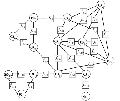
In order to compute the optimal estimate (5) in a distributed way, one can exploit the conditional independence structure of the joint distribution (6), which is conveniently revealed by factor graph (FG). FG is an undirected bipartite graphical representation of a joint distribution that unifies direct and undirected graphical models. An example of FG in the context of network-wide synchronization is shown in Fig. 3. In the FG, there are two distinct kinds of nodes. One is variable nodes representing local synchronization parameters 𝝎isubscript𝝎𝑖\bm{\omega}_{i}. If there is a communication link between node i𝑖i and node j𝑗j, the corresponding variable nodes 𝝎isubscript𝝎𝑖\bm{\omega}_{i} and 𝝎jsubscript𝝎𝑗\bm{\omega}_{j} are linked by the other kind of node, factor node fi,j=p(𝒓i,j|𝝎i,𝝎j)subscript𝑓𝑖𝑗𝑝conditionalsubscript𝒓𝑖𝑗subscript𝝎𝑖subscript𝝎𝑗f_{i,j}=p(\bm{r}_{i,j}|\bm{\omega}_{i},\bm{\omega}_{j}) representing the local likelihood function 111Note that fi,jsubscript𝑓𝑖𝑗f_{i,j}=fj,isubscript𝑓𝑗𝑖f_{j,i}.. On the other hand, the factor node fi=p(𝝎i)subscript𝑓𝑖𝑝subscript𝝎𝑖f_{i}=p(\bm{\omega}_{i}) denotes the prior distribution of frequency offsets of node i𝑖i, and is connected only to the variable node 𝝎isubscript𝝎𝑖\bm{\omega}_{i}. Note that the FG is bipartite which means neighbors of a factor node must be variable nodes and vice versa.

From the FG, two kinds of messages are passed around: One is the message from factor node f𝑓f (likelihood function fi,jsubscript𝑓𝑖𝑗f_{i,j} or prior distribution fisubscript𝑓𝑖f_{i}) to its neighboring variable node 𝝎isubscript𝝎𝑖\bm{\omega}_{i}, defined as the product of the function f𝑓f with messages received from all neighboring variable nodes except 𝝎isubscript𝝎𝑖\bm{\omega}_{i}, and then marginalized for 𝝎isubscript𝝎𝑖\bm{\omega}_{i} [34]

mfi(l)(𝝎i)=f×𝝎j(f)𝝎imjf(l1)(𝝎j)d{𝝎j}𝝎j(f)𝝎i,subscriptsuperscript𝑚𝑙𝑓𝑖subscript𝝎𝑖𝑓subscriptproductsubscript𝝎𝑗𝑓subscript𝝎𝑖subscriptsuperscript𝑚𝑙1𝑗𝑓subscript𝝎𝑗𝑑subscriptsubscript𝝎𝑗subscript𝝎𝑗𝑓subscript𝝎𝑖m^{(l)}_{f{\rightarrow}i}(\bm{\omega}_{i})=\int\cdots\int f\times\!\!\!\!\!\!\!\prod_{\bm{\omega}_{j}\in{\mathcal{B}}(f)\setminus\bm{\omega}_{i}}m^{(l-1)}_{j{\rightarrow}f}(\bm{\omega}_{j})d\{\bm{\omega}_{j}\}_{\bm{\omega}_{j}\in{\mathcal{B}}(f)\setminus\bm{\omega}_{i}}, (7)

where (f)𝑓{\mathcal{B}}(f) denotes the set of variable nodes that are direct neighbors of the factor nodes f𝑓f on the FG and (f)𝝎i𝑓subscript𝝎𝑖{{\mathcal{B}}(f)\setminus\bm{\omega}_{i}} denotes the same set but with 𝝎isubscript𝝎𝑖\bm{\omega}_{i} removed. In (7), mjf(l1)(𝝎j)subscriptsuperscript𝑚𝑙1𝑗𝑓subscript𝝎𝑗m^{(l-1)}_{j{\rightarrow}f}(\bm{\omega}_{j}) is the other kind of message from variable node to factor node which is simply the product of the incoming messages on other links, i.e.,

mjf(l)(𝝎j)=f~(𝝎j)fmf~j(l)(𝝎i),subscriptsuperscript𝑚𝑙𝑗𝑓subscript𝝎𝑗subscriptproduct~𝑓subscript𝝎𝑗𝑓subscriptsuperscript𝑚𝑙~𝑓𝑗subscript𝝎𝑖m^{(l)}_{j{\rightarrow}f}(\bm{\omega}_{j})=\prod_{\tilde{f}\in{\mathcal{B}}(\bm{\omega}_{j})\setminus f}m^{(l)}_{\tilde{f}{\rightarrow}j}(\bm{\omega}_{i}), (8)

where (𝝎j)subscript𝝎𝑗{\mathcal{B}}(\bm{\omega}_{j}) denotes the set of factor nodes that are direct neighbors of the variable nodes 𝝎jsubscript𝝎𝑗\bm{\omega}_{j} on the FG. It can be seen from (7) and (8) that for both variable nodes and factor nodes, each outgoing message is a function of all incoming messages in the last round except the incoming message from the node where the outgoing message will be directed to. This essential restriction guarantees that for cycle-free FG, incoming and outgoing messages on each edge are independent, and at the end the algorithm produces correct marginal posterior distribution.

The two kinds of messages are iteratively updated at variable nodes and factor nodes, respectively. In any round of message exchange, a belief of 𝝎isubscript𝝎𝑖\bm{\omega}_{i} can be computed at variable node i𝑖i as the product of all the incoming messages from neighboring factor nodes, which is given by

b(l)(𝝎i)=f(𝝎i)mfi(l)(𝝎i).superscript𝑏𝑙subscript𝝎𝑖subscriptproduct𝑓subscript𝝎𝑖subscriptsuperscript𝑚𝑙𝑓𝑖subscript𝝎𝑖b^{(l)}(\bm{\omega}_{i})=\prod_{f\in{\mathcal{B}}(\bm{\omega}_{i})}m^{(l)}_{f{\rightarrow}i}(\bm{\omega}_{i}). (9)

Thereupon, the estimate of 𝝎isubscript𝝎𝑖\bm{\omega}_{i} in the lthsuperscript𝑙𝑡l^{th} iteration is simply

𝝎^i(l)=𝝎ib(l)(𝝎i)𝑑𝝎i.superscriptsubscript^𝝎𝑖𝑙subscript𝝎𝑖superscript𝑏𝑙subscript𝝎𝑖differential-dsubscript𝝎𝑖\hat{\bm{\omega}}_{i}^{(l)}=\int\bm{\omega}_{i}b^{(l)}(\bm{\omega}_{i})d\bm{\omega}_{i}. (10)

Notice that after convergence, the belief b(l)(𝝎i)superscript𝑏𝑙subscript𝝎𝑖b^{(l)}(\bm{\omega}_{i}) at each variable node corresponds to the marginal distribution of that variable exactly when the underlying FG is loop free [34]. However, for the FG with loops, it is generally difficult to known if BP will converge [36]. Even if BP converge to a fixed point, there is no guarantee on the estimation accuracy. Despite the lack of general results on BP, in this paper, the convergence and optimality of BP for network-wide CFO estimation algorithm will be proved in section IV.

III-B Message Computation

In the BP framework, messages are passed and updated iteratively. In order to start the recursion, in the first round of message passing, it is reasonable to set the initial messages from factor nodes to variable nodes mfii(0)(𝝎i)subscriptsuperscript𝑚0subscript𝑓𝑖𝑖subscript𝝎𝑖m^{(0)}_{f_{i}{\rightarrow}i}(\bm{\omega}_{i}) and mfi,ji(0)(𝝎i)subscriptsuperscript𝑚0subscript𝑓𝑖𝑗𝑖subscript𝝎𝑖m^{(0)}_{f_{i,j}{\rightarrow}i}(\bm{\omega}_{i}) as p(𝝎i)𝑝subscript𝝎𝑖p(\bm{\omega}_{i}) and non-informative message 𝒩(𝝎i;𝒗fi,ji(0),𝑪fi,ji(0))𝒩subscript𝝎𝑖subscriptsuperscript𝒗0subscript𝑓𝑖𝑗𝑖superscriptsubscript𝑪subscript𝑓𝑖𝑗𝑖0\mathcal{N}(\bm{\omega}_{i};\bm{v}^{(0)}_{f_{i,j}{\rightarrow}i},\bm{C}_{f_{i,j}{\rightarrow}i}^{(0)}), respectively, where 𝒗fi,ji(0)subscriptsuperscript𝒗0subscript𝑓𝑖𝑗𝑖\bm{v}^{(0)}_{f_{i,j}{\rightarrow}i} can be arbitrarily chosen and [𝑪fi,ji(0))]1=𝟎[\bm{C}_{f_{i,j}{\rightarrow}i}^{(0)})]^{-1}=\bm{0}. Assuming p(𝝎i)=mfi,ji(0)(𝝎i)𝑝subscript𝝎𝑖subscriptsuperscript𝑚0subscript𝑓𝑖𝑗𝑖subscript𝝎𝑖p(\bm{\omega}_{i})=m^{(0)}_{f_{i,j}{\rightarrow}i}(\bm{\omega}_{i}) is in Gaussian form 𝒩(𝝎i;𝒗i,𝑪i)𝒩subscript𝝎𝑖subscript𝒗𝑖subscript𝑪𝑖{\mathcal{N}}(\bm{\omega}_{i};\bm{v}_{i},\bm{C}_{i}) (if there is no prior information, we can set the mean to be zero and set the variance to be a large value, i.e., non-informative prior). Thereupon, based on the fact that the likelihood function fi,jsubscript𝑓𝑖𝑗f_{i,j} is also Gaussian, according to (7), mfi,ji(1)(𝝎i)subscriptsuperscript𝑚1subscript𝑓𝑖𝑗𝑖subscript𝝎𝑖m^{(1)}_{f_{i,j}{\rightarrow}i}(\bm{\omega}_{i}) is a Gaussian function. In addition, mjfi,j(1)(𝝎j)subscriptsuperscript𝑚1𝑗subscript𝑓𝑖𝑗subscript𝝎𝑗m^{(1)}_{j{\rightarrow}f_{i,j}}(\bm{\omega}_{j}) being the product of Gaussian functions in (8) is also a Gaussian function [38]. Thus during each round of message exchange, all the messages are Gaussian functions and only the mean vectors and covariance matrices need to be exchanged between factor nodes and variable nodes.

At this point, we can compute the messages at any iteration. In general, for the lthsuperscript𝑙𝑡l^{th} (l=2,3,𝑙23l=2,3,\cdots) round of message exchange, factor node fi,jsubscript𝑓𝑖𝑗f_{i,j} receive messages mjfi,j(l1)(𝝎j)subscriptsuperscript𝑚𝑙1𝑗subscript𝑓𝑖𝑗subscript𝝎𝑗m^{(l-1)}_{j{\rightarrow}f_{i,j}}(\bm{\omega}_{j}) from its neighboring variable nodes and then compute messages using (7). After some derivations, it can be obtained that

mfi,ji(l)(𝝎i)subscriptsuperscript𝑚𝑙subscript𝑓𝑖𝑗𝑖subscript𝝎𝑖\displaystyle m^{(l)}_{f_{i,j}{\rightarrow}i}(\bm{\omega}_{i}) =\displaystyle= p(𝑨i,j,𝑨j,i|𝝎i,𝝎j)mjfi,j(l1)(𝝎j)𝑑𝝎j𝑝subscript𝑨𝑖𝑗conditionalsubscript𝑨𝑗𝑖subscript𝝎𝑖subscript𝝎𝑗subscriptsuperscript𝑚𝑙1𝑗subscript𝑓𝑖𝑗subscript𝝎𝑗differential-dsubscript𝝎𝑗\displaystyle\int p(\bm{A}_{i,j},\bm{A}_{j,i}|\bm{\omega}_{i},\bm{\omega}_{j})m^{(l-1)}_{j{\rightarrow}f_{i,j}}(\bm{\omega}_{j})d\bm{\omega}_{j} (11)
proportional-to\displaystyle\propto 𝒩(𝝎i;𝒗fi,ji(l),𝑪fi,ji(l)),𝒩subscript𝝎𝑖subscriptsuperscript𝒗𝑙subscript𝑓𝑖𝑗𝑖superscriptsubscript𝑪subscript𝑓𝑖𝑗𝑖𝑙\displaystyle\mathcal{N}(\bm{\omega}_{i};\bm{v}^{(l)}_{f_{i,j}{\rightarrow}i},\bm{C}_{f_{i,j}{\rightarrow}i}^{(l)}),

where the inverse of covariance matrix is

[𝑪fi,ji(l)]1=𝑨i,jT[𝑹i,j+𝑨j,i𝑪jfi,j(l1)𝑨j,iT]1𝑨i,j,superscriptdelimited-[]superscriptsubscript𝑪subscript𝑓𝑖𝑗𝑖𝑙1superscriptsubscript𝑨𝑖𝑗𝑇superscriptdelimited-[]subscript𝑹𝑖𝑗subscript𝑨𝑗𝑖superscriptsubscript𝑪𝑗subscript𝑓𝑖𝑗𝑙1superscriptsubscript𝑨𝑗𝑖𝑇1subscript𝑨𝑖𝑗\big{[}\bm{C}_{f_{i,j}{\rightarrow}i}^{(l)}\big{]}^{-1}=\bm{A}_{i,j}^{T}\bigg{[}\bm{R}_{i,j}+\bm{A}_{j,i}\bm{C}_{j{\rightarrow}f_{i,j}}^{(l-1)}\bm{A}_{j,i}^{T}\bigg{]}^{-1}\bm{A}_{i,j}, (12)

and the mean vector is

𝒗fi,ji(l)=𝑪fi,ji(l)𝑨i,jT[𝑹i,j+𝑨j,i𝑪jfi,j(l1)𝑨j,iT]1(𝒓i,j𝑨j,i𝒗jfi,j(l1)).subscriptsuperscript𝒗𝑙subscript𝑓𝑖𝑗𝑖superscriptsubscript𝑪subscript𝑓𝑖𝑗𝑖𝑙superscriptsubscript𝑨𝑖𝑗𝑇superscriptdelimited-[]subscript𝑹𝑖𝑗subscript𝑨𝑗𝑖superscriptsubscript𝑪𝑗subscript𝑓𝑖𝑗𝑙1superscriptsubscript𝑨𝑗𝑖𝑇1subscript𝒓𝑖𝑗subscript𝑨𝑗𝑖subscriptsuperscript𝒗𝑙1𝑗subscript𝑓𝑖𝑗\bm{v}^{(l)}_{f_{i,j}{\rightarrow}i}=\bm{C}_{f_{i,j}{\rightarrow}i}^{(l)}\bm{A}_{i,j}^{T}\bigg{[}\bm{R}_{i,j}+\bm{A}_{j,i}\bm{C}_{j{\rightarrow}f_{i,j}}^{(l-1)}\bm{A}_{j,i}^{T}\bigg{]}^{-1}(\bm{r}_{i,j}-\bm{A}_{j,i}\bm{v}^{(l-1)}_{j{\rightarrow}f_{i,j}}). (13)

On the other hand, using (8), the messages passed from variable nodes to factor nodes can be computed as

mifi,j(l)(𝝎i)subscriptsuperscript𝑚𝑙𝑖subscript𝑓𝑖𝑗subscript𝝎𝑖\displaystyle m^{(l)}_{i{\rightarrow}f_{i,j}}(\bm{\omega}_{i}) =\displaystyle= f(𝝎i)fi,jmfi(l)(𝝎i)subscriptproduct𝑓subscript𝝎𝑖subscript𝑓𝑖𝑗subscriptsuperscript𝑚𝑙𝑓𝑖subscript𝝎𝑖\displaystyle\prod_{f\in{\mathcal{B}}(\bm{\omega}_{i})\setminus f_{i,j}}m^{(l)}_{f{\rightarrow}i}(\bm{\omega}_{i}) (14)
proportional-to\displaystyle\propto 𝒩(𝝎i;𝒗ifi,j(l),𝑪ifi,j(l)),𝒩subscript𝝎𝑖subscriptsuperscript𝒗𝑙𝑖subscript𝑓𝑖𝑗subscriptsuperscript𝑪𝑙𝑖subscript𝑓𝑖𝑗\displaystyle\mathcal{N}(\bm{\omega}_{i};\bm{v}^{(l)}_{i{\rightarrow}f_{i,j}},\bm{C}^{(l)}_{i{\rightarrow}f_{i,j}}),

where

[𝑪ifi,j(l)]1=f(𝝎i)fi,j[𝑪fi(l)]1,superscriptdelimited-[]subscriptsuperscript𝑪𝑙𝑖subscript𝑓𝑖𝑗1subscript𝑓subscript𝝎𝑖subscript𝑓𝑖𝑗superscriptdelimited-[]superscriptsubscript𝑪𝑓𝑖𝑙1\big{[}\bm{C}^{(l)}_{i{\rightarrow}f_{i,j}}]^{-1}=\sum_{f\in{\mathcal{B}}(\bm{\omega}_{i})\setminus f_{i,j}}\big{[}\bm{C}_{f{\rightarrow}i}^{(l)}\big{]}^{-1}, (15)

and

𝒗ifi,j(l)=𝑪ifi,j(l)f(𝝎i)fi,j[𝑪fi(l)]1𝒗fi(l).subscriptsuperscript𝒗𝑙𝑖subscript𝑓𝑖𝑗subscriptsuperscript𝑪𝑙𝑖subscript𝑓𝑖𝑗subscript𝑓subscript𝝎𝑖subscript𝑓𝑖𝑗superscriptdelimited-[]superscriptsubscript𝑪𝑓𝑖𝑙1subscriptsuperscript𝒗𝑙𝑓𝑖\bm{v}^{(l)}_{i{\rightarrow}f_{i,j}}=\bm{C}^{(l)}_{i{\rightarrow}f_{i,j}}\sum_{f\in{\mathcal{B}}(\bm{\omega}_{i})\setminus f_{i,j}}\big{[}\bm{C}_{f{\rightarrow}i}^{(l)}\big{]}^{-1}\bm{v}^{(l)}_{f{\rightarrow}i}. (16)

Furthermore, during each round of message passing, each node can compute the belief for 𝝎isubscript𝝎𝑖\bm{\omega}_{i} using (9), which can be easily shown to be bi(l)(𝝎i)𝒩(𝝎i;𝝁i(l),𝑷i(l))similar-tosuperscriptsubscript𝑏𝑖𝑙subscript𝝎𝑖𝒩subscript𝝎𝑖superscriptsubscript𝝁𝑖𝑙superscriptsubscript𝑷𝑖𝑙b_{i}^{(l)}(\bm{\omega}_{i})\sim\mathcal{N}(\bm{\omega}_{i};\bm{\mu}_{i}^{(l)},\bm{P}_{i}^{(l)}), with the inverse of covariance matrix

[𝑷i(l)]1=j(i)[𝑪fi,ji(l)]1,superscriptdelimited-[]superscriptsubscript𝑷𝑖𝑙1subscript𝑗𝑖superscriptdelimited-[]superscriptsubscript𝑪subscript𝑓𝑖𝑗𝑖𝑙1\big{[}\bm{P}_{i}^{(l)}\big{]}^{-1}=\sum_{j\in{\mathcal{I}}(i)}\big{[}\bm{C}_{f_{i,j}{\rightarrow}i}^{(l)}\big{]}^{-1}, (17)

and mean vector

𝝁i(l)=𝑷i(l)j(i)[𝑪fi,ji(l)]1𝒗fi,ji(l).superscriptsubscript𝝁𝑖𝑙superscriptsubscript𝑷𝑖𝑙subscript𝑗𝑖superscriptdelimited-[]superscriptsubscript𝑪subscript𝑓𝑖𝑗𝑖𝑙1subscriptsuperscript𝒗𝑙subscript𝑓𝑖𝑗𝑖\bm{\mu}_{i}^{(l)}=\bm{P}_{i}^{(l)}\sum_{j\in{\mathcal{I}}(i)}\big{[}\bm{C}_{f_{i,j}{\rightarrow}i}^{(l)}\big{]}^{-1}\bm{v}^{(l)}_{f_{i,j}{\rightarrow}i}. (18)

When the algorithm converges or the maximum number of message exchange is reached, each node computes the CFOs according to (10) as

𝝎^i(l)=𝝎ib(l)(𝝎i)𝑑𝝎i=𝝁i(l).superscriptsubscript^𝝎𝑖𝑙subscript𝝎𝑖superscript𝑏𝑙subscript𝝎𝑖differential-dsubscript𝝎𝑖superscriptsubscript𝝁𝑖𝑙\hat{\bm{\omega}}_{i}^{(l)}=\int\bm{\omega}_{i}b^{(l)}(\bm{\omega}_{i})d\bm{\omega}_{i}=\bm{\mu}_{i}^{(l)}. (19)

The iterative algorithm based on BP is summarized as follows. The algorithm is started by setting the message from factor node to variable node as mfii(0)(𝝎i)=p(𝝎i)subscriptsuperscript𝑚0subscript𝑓𝑖𝑖subscript𝝎𝑖𝑝subscript𝝎𝑖m^{(0)}_{f_{i}{\rightarrow}i}(\bm{\omega}_{i})=p(\bm{\omega}_{i}) and mfi,ji(0)(𝝎i)=𝒩(𝝎i;𝒗fi,ji(0),𝑪fi,ji(0))subscriptsuperscript𝑚0subscript𝑓𝑖𝑗𝑖subscript𝝎𝑖𝒩subscript𝝎𝑖subscriptsuperscript𝒗0subscript𝑓𝑖𝑗𝑖superscriptsubscript𝑪subscript𝑓𝑖𝑗𝑖0m^{(0)}_{f_{i,j}{\rightarrow}i}(\bm{\omega}_{i})=\mathcal{N}(\bm{\omega}_{i};\bm{v}^{(0)}_{f_{i,j}{\rightarrow}i},\bm{C}_{f_{i,j}{\rightarrow}i}^{(0)}) with 𝒗fi,ji(0)=𝟎subscriptsuperscript𝒗0subscript𝑓𝑖𝑗𝑖0\bm{v}^{(0)}_{f_{i,j}{\rightarrow}i}=\bm{0} and [𝑪fi,ji(0))]1=𝟎[\bm{C}_{f_{i,j}{\rightarrow}i}^{(0)})]^{-1}=\bm{0}. At each round of message exchange, every variable node computes the output messages to factor nodes according to (15) and (16). After receiving the messages from its neighboring variable nodes, each factor node computes its output messages according to (12) and (13). Such iteration is terminated when (18) converges (e.g., when μi(l)μi(l1)<ηnormsuperscriptsubscript𝜇𝑖𝑙superscriptsubscript𝜇𝑖𝑙1𝜂\|\mu_{i}^{(l)}-\mu_{i}^{(l-1)}\|<\eta, where η𝜂\eta is a threshold) or the maximum number of iteration is reached. Then the estimate of CFOs of each node is obtained as in (19).

Remark 3

In practical networks, there is neither factor nodes nor variable nodes. The two kinds of messages mifi,j(l)(𝛚i)subscriptsuperscript𝑚𝑙𝑖subscript𝑓𝑖𝑗subscript𝛚𝑖m^{(l)}_{i{\rightarrow}f_{i,j}}(\bm{\omega}_{i}) and mfi,jj(l)(𝛚j)subscriptsuperscript𝑚𝑙subscript𝑓𝑖𝑗𝑗subscript𝛚𝑗m^{(l)}_{f_{i,j}{\rightarrow}j}(\bm{\omega}_{j}) are computed locally at node i𝑖i, and only mean vector 𝐯fi,jj(l)(𝛚j)subscriptsuperscript𝐯𝑙subscript𝑓𝑖𝑗𝑗subscript𝛚𝑗\bm{v}^{(l)}_{f_{i,j}{\rightarrow}j}(\bm{\omega}_{j}) and covariance matrix 𝐂fi,jj(l)(𝛚j)superscriptsubscript𝐂subscript𝑓𝑖𝑗𝑗𝑙subscript𝛚𝑗\bm{C}_{f_{i,j}{\rightarrow}j}^{(l)}(\bm{\omega}_{j}) are passed from node i𝑖i to node j𝑗j during each round of message exchange of BP. It can be seen the algorithm is fully distributed and each node only needs to exchange limited information with neighboring nodes.

Remark 4

Since each pair of node has knowledge of relative CFOs and channel between them, the BP message exchange can be performed as in point-to-point communications.

IV Theoretical Analyses of BP method

It is generally known that if the FG contains cycles, such as the one shown in Fig. 3, messages can flow many times around the graph, leading to the possibility of divergence of BP algorithm [35]. A general sufficient condition for convergence of loopy FGs is given in [36]. Unfortunately, it requires the knowledge of the joint posterior distribution of all unknown variables as shown in (6), and is difficult to verify for large-scale dynamic networks. Recently, [37] proved the convergence of BP in the context of distributed clock offset synchronization in wireless sensor network. The convergence is established for scalar variables in which sub-stochastic and irreducible properties of BP message recursion were exploited. However, in vector variable case, the BP messages involve matrix inverses (see (12), (13), (15) and (16)), and the sub-stochastic and irreducible properties cannot be easily applied. In the following, we will prove the convergence of BP messages in vector form, and show that the BP based CFO estimates asymptotically converge to the optimal MMSE solution regardless of network topology.

Theorem 1. The covariance matrix 𝑷i(l)superscriptsubscript𝑷𝑖𝑙\bm{P}_{i}^{(l)} of belief bi(l)(𝝎i)superscriptsubscript𝑏𝑖𝑙subscript𝝎𝑖b_{i}^{(l)}(\bm{\omega}_{i}) at each node converges, and there exists a positive definite matrix 𝑷isuperscriptsubscript𝑷𝑖{\bm{P}_{i}^{\ast}} such that liml+𝑷i(l)=𝑷isubscript𝑙superscriptsubscript𝑷𝑖𝑙superscriptsubscript𝑷𝑖\lim_{l\to+\infty}\bm{P}_{i}^{(l)}=\bm{P}_{i}^{\ast} regardless of network topology.

Proof: We begin with a few properties of positive semi-definite (p.s.d.) matrices and positive definite (p.d.) matrices. If 𝑿𝑿\bm{X}, 𝒀𝒀\bm{Y}, 𝒁𝒁\bm{Z} are Nisubscript𝑁𝑖N_{i}-by-Nisubscript𝑁𝑖N_{i} matrices and 𝑿𝟎succeeds𝑿0\bm{X}\succ\bm{0}, 𝒀𝟎succeeds𝒀0\bm{Y}\succ\bm{0}, 𝒁𝟎succeeds-or-equals𝒁0\bm{Z}\succeq\bm{0}, then we have

Property i): 𝑿10succeedssuperscript𝑿10\bm{X}^{-1}\succ 0.

Property ii): 𝑿+𝒀0succeeds𝑿𝒀0\bm{X}+\bm{Y}\succ 0.

Property iii): 𝑿+𝒁0succeeds𝑿𝒁0\bm{X}+\bm{Z}\succ 0.

Property iv): 𝑿𝒀succeeds-or-equals𝑿𝒀\bm{X}\succeq\bm{Y} if and only if 𝒀1𝑿1succeeds-or-equalssuperscript𝒀1superscript𝑿1\bm{Y}^{-1}\succeq\bm{X}^{-1} [39].

Property v): 𝑨i,jT𝑿𝑨i,j𝟎succeedssuperscriptsubscript𝑨𝑖𝑗𝑇𝑿subscript𝑨𝑖𝑗0\bm{A}_{i,j}^{T}\bm{X}\bm{A}_{i,j}\succ\bm{0} and 𝑨i,jT𝒁𝑨i,j𝟎succeeds-or-equalssuperscriptsubscript𝑨𝑖𝑗𝑇𝒁subscript𝑨𝑖𝑗0\bm{A}_{i,j}^{T}\bm{Z}\bm{A}_{i,j}\succeq\bm{0}, where 𝑨i,jsubscript𝑨𝑖𝑗\bm{A}_{i,j} is defined in (4).

Property vi): 𝑨j,i𝑿𝑨j,iT0succeeds-or-equalssubscript𝑨𝑗𝑖𝑿subscriptsuperscript𝑨𝑇𝑗𝑖0\bm{A}_{j,i}\bm{X}\bm{A}^{T}_{j,i}\succeq 0.

Properties i) to iv) are standard results in matrix analysis. Property v) is true due to the fact that 𝑨i,jsubscript𝑨𝑖𝑗\bm{A}_{i,j} is of full column rank. The proof of vi) follows from the definition of 𝑿𝟎succeeds𝑿0\bm{X}\succ\bm{0} which is 𝒚T𝑿𝒚0superscript𝒚𝑇𝑿𝒚0\bm{y}^{T}\bm{X}\bm{y}\geq 0 for any 𝒚𝒚\bm{y} (including all zeros vector). The result is obtained if we let 𝒚=𝑨j,iT𝒙𝒚superscriptsubscript𝑨𝑗𝑖𝑇𝒙\bm{y}=\bm{A}_{j,i}^{T}\bm{x}.

Next, we investigate the updating properties of the message covariance matrix. Substituting (15) into (12), the covariance update rules from factor nodes to variable nodes are

[𝑪fi,ji(l)]1=𝑨i,jT[𝑹i,j+𝑨j,i[𝑪fjj1+fk,j(𝝎j)fi,j[𝑪fk,jj(l1)]1]1𝑨j,iT]1𝑨i,j.superscriptdelimited-[]superscriptsubscript𝑪subscript𝑓𝑖𝑗𝑖𝑙1superscriptsubscript𝑨𝑖𝑗𝑇superscriptdelimited-[]subscript𝑹𝑖𝑗subscript𝑨𝑗𝑖superscriptdelimited-[]superscriptsubscript𝑪subscript𝑓𝑗𝑗1subscriptsubscript𝑓𝑘𝑗subscript𝝎𝑗subscript𝑓𝑖𝑗superscriptdelimited-[]superscriptsubscript𝑪subscript𝑓𝑘𝑗𝑗𝑙111superscriptsubscript𝑨𝑗𝑖𝑇1subscript𝑨𝑖𝑗\big{[}\bm{C}_{f_{i,j}{\rightarrow}i}^{(l)}\big{]}^{-1}=\bm{A}_{i,j}^{T}\bigg{[}\bm{R}_{i,j}+\bm{A}_{j,i}\bigg{[}\bm{C}_{f_{j}{\rightarrow}j}^{-1}+\sum_{f_{k,j}\in{\mathcal{B}}(\bm{\omega}_{j})\setminus f_{i,j}}\big{[}\bm{C}_{f_{k,j}{\rightarrow}j}^{(l-1)}\big{]}^{-1}\bigg{]}^{-1}\bm{A}_{j,i}^{T}\bigg{]}^{-1}\bm{A}_{i,j}. (20)

From (20), we can deduce two consequences. First, if all message covariance 𝑪fk,jj(l1)superscriptsubscript𝑪subscript𝑓𝑘𝑗𝑗𝑙1\bm{C}_{f_{k,j}{\rightarrow}j}^{(l-1)} and prior covariance 𝑪fjjsubscript𝑪subscript𝑓𝑗𝑗\bm{C}_{f_{j}{\rightarrow}j} on the right-hand-side of (20) are non-informative, [𝑪fi,ji(l)]1superscriptdelimited-[]superscriptsubscript𝑪subscript𝑓𝑖𝑗𝑖𝑙1\big{[}\bm{C}_{f_{i,j}{\rightarrow}i}^{(l)}\big{]}^{-1} cannot be updated, i.e., [𝑪fi,ji(l)]1=𝟎superscriptdelimited-[]superscriptsubscript𝑪subscript𝑓𝑖𝑗𝑖𝑙10\big{[}\bm{C}_{f_{i,j}{\rightarrow}i}^{(l)}\big{]}^{-1}=\bm{0}. On the other hand, if some of the [𝑪fk,jj(l1)]1superscriptdelimited-[]superscriptsubscript𝑪subscript𝑓𝑘𝑗𝑗𝑙11[\bm{C}_{f_{k,j}{\rightarrow}j}^{(l-1)}]^{-1} or 𝑪fjj1superscriptsubscript𝑪subscript𝑓𝑗𝑗1\bm{C}_{f_{j}{\rightarrow}j}^{-1} on the right-hand-side of (20) are p.d. while the remaining are 𝟎0\bm{0}, then [𝑪fjj1+fk,j(𝝎j)fi,j[𝑪fk,jj(l1)]1]1𝟎succeedssuperscriptdelimited-[]superscriptsubscript𝑪subscript𝑓𝑗𝑗1subscriptsubscript𝑓𝑘𝑗subscript𝝎𝑗subscript𝑓𝑖𝑗superscriptdelimited-[]superscriptsubscript𝑪subscript𝑓𝑘𝑗𝑗𝑙1110\big{[}\bm{C}_{f_{j}{\rightarrow}j}^{-1}+\sum_{f_{k,j}\in{\mathcal{B}}(\bm{\omega}_{j})\setminus f_{i,j}}\big{[}\bm{C}_{f_{k,j}{\rightarrow}j}^{(l-1)}\big{]}^{-1}\big{]}^{-1}\succ\bm{0} according to property iii). Applying property vi), we have 𝑨j,i[𝑪fjj1+fk,j(𝝎j)fi,j[𝑪fk,jj(l1)]1]1𝑨j,iT0succeeds-or-equalssubscript𝑨𝑗𝑖superscriptdelimited-[]superscriptsubscript𝑪subscript𝑓𝑗𝑗1subscriptsubscript𝑓𝑘𝑗subscript𝝎𝑗subscript𝑓𝑖𝑗superscriptdelimited-[]superscriptsubscript𝑪subscript𝑓𝑘𝑗𝑗𝑙111superscriptsubscript𝑨𝑗𝑖𝑇0\bm{A}_{j,i}\bigg{[}\bm{C}_{f_{j}{\rightarrow}j}^{-1}+\sum_{f_{k,j}\in{\mathcal{B}}(\bm{\omega}_{j})\setminus f_{i,j}}\big{[}\bm{C}_{f_{k,j}{\rightarrow}j}^{(l-1)}\big{]}^{-1}\bigg{]}^{-1}\bm{A}_{j,i}^{T}\succeq 0. Furthermore, since 𝑹i,jsubscript𝑹𝑖𝑗\bm{R}_{i,j} is the relative CFO estimation covariance, we have 𝑹i,j𝟎succeedssubscript𝑹𝑖𝑗0\bm{R}_{i,j}\succ\bm{0}. Thus, 𝑹i,j+𝑨j,i[𝑪fjj1+fk,j(𝝎j)fi,j[𝑪fk,jj(l1)]1]1𝑨j,iT𝟎succeedssubscript𝑹𝑖𝑗subscript𝑨𝑗𝑖superscriptdelimited-[]superscriptsubscript𝑪subscript𝑓𝑗𝑗1subscriptsubscript𝑓𝑘𝑗subscript𝝎𝑗subscript𝑓𝑖𝑗superscriptdelimited-[]superscriptsubscript𝑪subscript𝑓𝑘𝑗𝑗𝑙111superscriptsubscript𝑨𝑗𝑖𝑇0\bm{R}_{i,j}+\bm{A}_{j,i}\bigg{[}\bm{C}_{f_{j}{\rightarrow}j}^{-1}+\sum_{f_{k,j}\in{\mathcal{B}}(\bm{\omega}_{j})\setminus f_{i,j}}\big{[}\bm{C}_{f_{k,j}{\rightarrow}j}^{(l-1)}\big{]}^{-1}\bigg{]}^{-1}\bm{A}_{j,i}^{T}\succ\bm{0}. Then, based on properties i) and v), we obtain [𝑪fi,ji(l)]1𝟎succeedssuperscriptdelimited-[]superscriptsubscript𝑪subscript𝑓𝑖𝑗𝑖𝑙10\big{[}\bm{C}_{f_{i,j}{\rightarrow}i}^{(l)}\big{]}^{-1}\succ\bm{0}. We summarize the above discussion as

[𝑪fi,ji(l)]1{=𝟎,if all [𝑪fk,jj(l1)]1 and 𝑪fjj1=𝟎 ,𝟎,if some of [𝑪fk,jj(l1)]1 or 𝑪fjj1𝟎, while others are 𝟎.superscriptdelimited-[]superscriptsubscript𝑪subscript𝑓𝑖𝑗𝑖𝑙1casesabsent0if all [𝑪fk,jj(l1)]1 and 𝑪fjj1=𝟎 succeedsabsent0if some of [𝑪fk,jj(l1)]1 or 𝑪fjj1𝟎, while others are 𝟎\big{[}\bm{C}_{f_{i,j}{\rightarrow}i}^{(l)}\big{]}^{-1}\left\{\begin{array}[]{l}=\bm{0},\quad\textrm{if all $[\bm{C}_{f_{k,j}{\rightarrow}j}^{(l-1)}]^{-1}$ and $\bm{C}_{f_{j}{\rightarrow}j}^{-1}=\bm{0}$ },\\ \succ\bm{0},\quad\textrm{if some of $[\bm{C}_{f_{k,j}{\rightarrow}j}^{(l-1)}]^{-1}$ or $\bm{C}_{f_{j}{\rightarrow}j}^{-1}\succ\bm{0}$, while others are $\bm{0}$}.\end{array}\right. (21)

Now we prove that for any node i𝑖i, if there exists a directed path from node 1ji1𝑗𝑖1{\rightarrow}\ldots{\rightarrow}j{\rightarrow}i in the network topology, there must be a finite iteration number s𝑠s such that [𝑪fi,ji(s+1)]1[𝑪fi,ji(s)]1[𝑪fi,ji(s1)]1=𝟎.succeeds-or-equalssuperscriptdelimited-[]superscriptsubscript𝑪subscript𝑓𝑖𝑗𝑖𝑠11superscriptdelimited-[]superscriptsubscript𝑪subscript𝑓𝑖𝑗𝑖𝑠1succeedssuperscriptdelimited-[]superscriptsubscript𝑪subscript𝑓𝑖𝑗𝑖𝑠110\big{[}\bm{C}_{f_{i,j}{\rightarrow}i}^{(s+1)}\big{]}^{-1}\succeq\big{[}\bm{C}_{f_{i,j}{\rightarrow}i}^{(s)}\big{]}^{-1}\succ\big{[}\bm{C}_{f_{i,j}{\rightarrow}i}^{(s-1)}\big{]}^{-1}=\bm{0}. Initially, all [𝑪fk,jj(0)]1superscriptdelimited-[]superscriptsubscript𝑪subscript𝑓𝑘𝑗𝑗01[\bm{C}_{f_{k,j}{\rightarrow}j}^{(0)}]^{-1} and 𝑪fjj1superscriptsubscript𝑪subscript𝑓𝑗𝑗1\bm{C}_{f_{j}{\rightarrow}j}^{-1} over the FG equal 𝟎0\bm{0} except 𝑪f111=𝑰superscriptsubscript𝑪subscript𝑓111𝑰\bm{C}_{f_{1}{\rightarrow}1}^{-1}=\infty\bm{I} at the reference node. Hence, the message update starts from the reference node. More explicitly, ifor-all𝑖\forall i: {i,1}𝑖1\{i,1\}\in\mathcal{E}, the message covariance is obtained by putting j=1𝑗1j=1 into (20), which is

[𝑪fi,1i(1)]1=𝑨i,1T𝑹i,11𝑨i,1𝟎,superscriptdelimited-[]superscriptsubscript𝑪subscript𝑓𝑖1𝑖11superscriptsubscript𝑨𝑖1𝑇superscriptsubscript𝑹𝑖11subscript𝑨𝑖1succeeds0\big{[}\bm{C}_{f_{i,1}{\rightarrow}i}^{(1)}\big{]}^{-1}=\bm{A}_{i,1}^{T}\bm{R}_{i,1}^{-1}\bm{A}_{i,1}\succ\bm{0}, (22)

where the p.d. property is due to property v). Furthermore, since 𝑪f111=𝑰superscriptsubscript𝑪subscript𝑓111𝑰\bm{C}_{f_{1}{\rightarrow}1}^{-1}=\infty\bm{I}, it will dominate the sum 𝑪fjj1+fk,j(𝝎j)fi,j[𝑪fk,jj(l1)]1superscriptsubscript𝑪subscript𝑓𝑗𝑗1subscriptsubscript𝑓𝑘𝑗subscript𝝎𝑗subscript𝑓𝑖𝑗superscriptdelimited-[]superscriptsubscript𝑪subscript𝑓𝑘𝑗𝑗𝑙11\bm{C}_{f_{j}{\rightarrow}j}^{-1}+\sum_{f_{k,j}\in{\mathcal{B}}(\bm{\omega}_{j})\setminus f_{i,j}}\big{[}\bm{C}_{f_{k,j}{\rightarrow}j}^{(l-1)}\big{]}^{-1} in (20), and lead to [𝑪fi,1i(l)]1=𝑨i,1T𝑹i,11𝑨i,1superscriptdelimited-[]superscriptsubscript𝑪subscript𝑓𝑖1𝑖𝑙1superscriptsubscript𝑨𝑖1𝑇superscriptsubscript𝑹𝑖11subscript𝑨𝑖1\big{[}\bm{C}_{f_{i,1}{\rightarrow}i}^{(l)}\big{]}^{-1}=\bm{A}_{i,1}^{T}\bm{R}_{i,1}^{-1}\bm{A}_{i,1}. Thus, we have

=[𝑪fi,1i(l)]1==[𝑪fi,1i(2)]1=[𝑪fi,1i(1)]1[𝑪fi,1i(0)]1=𝟎.superscriptdelimited-[]superscriptsubscript𝑪subscript𝑓𝑖1𝑖𝑙1superscriptdelimited-[]superscriptsubscript𝑪subscript𝑓𝑖1𝑖21superscriptdelimited-[]superscriptsubscript𝑪subscript𝑓𝑖1𝑖11succeedssuperscriptdelimited-[]superscriptsubscript𝑪subscript𝑓𝑖1𝑖010\ldots=\big{[}\bm{C}_{f_{i,1}{\rightarrow}i}^{(l)}\big{]}^{-1}=\ldots=\big{[}\bm{C}_{f_{i,1}{\rightarrow}i}^{(2)}\big{]}^{-1}=\big{[}\bm{C}_{f_{i,1}{\rightarrow}i}^{(1)}\big{]}^{-1}\succ\big{[}\bm{C}_{f_{i,1}{\rightarrow}i}^{(0)}\big{]}^{-1}=\bm{0}. (23)

Then, we consider all nodes i𝑖i with a directed path node 1ji1𝑗𝑖1{\rightarrow}j{\rightarrow}i. In the 1stsuperscript1𝑠𝑡1^{st} iteration, node j𝑗j will take the position of node i𝑖i in (23) implying [𝑪fj,1j(1)]1𝟎succeedssuperscriptdelimited-[]superscriptsubscript𝑪subscript𝑓𝑗1𝑗110\big{[}\bm{C}_{f_{j,1}{\rightarrow}j}^{(1)}\big{]}^{-1}\succ\bm{0}, while [𝑪fi,ji(1)]1superscriptdelimited-[]superscriptsubscript𝑪subscript𝑓𝑖𝑗𝑖11\big{[}\bm{C}_{f_{i,j}{\rightarrow}i}^{(1)}\big{]}^{-1} has not been updated in the first iteration, i.e., [𝑪fi,ji(1)]1=𝟎superscriptdelimited-[]superscriptsubscript𝑪subscript𝑓𝑖𝑗𝑖110\big{[}\bm{C}_{f_{i,j}{\rightarrow}i}^{(1)}\big{]}^{-1}=\bm{0}. In the second iteration, from (21), we have [𝑪fi,ji(2)]1𝟎succeedssuperscriptdelimited-[]superscriptsubscript𝑪subscript𝑓𝑖𝑗𝑖210\big{[}\bm{C}_{f_{i,j}{\rightarrow}i}^{(2)}\big{]}^{-1}\succ\bm{0}. Since [𝑪fk,jj(1)]1superscriptdelimited-[]superscriptsubscript𝑪subscript𝑓𝑘𝑗𝑗11\big{[}\bm{C}_{f_{k,j}{\rightarrow}j}^{(1)}\big{]}^{-1} and 𝑪fjj1superscriptsubscript𝑪subscript𝑓𝑗𝑗1\bm{C}_{f_{j}{\rightarrow}j}^{-1} equal 𝟎0\bm{0}, taking inverse on 𝑪fjj1+fk,j(𝝎j)fi,j[𝑪fk,jj(1)]1superscriptsubscript𝑪subscript𝑓𝑗𝑗1subscriptsubscript𝑓𝑘𝑗subscript𝝎𝑗subscript𝑓𝑖𝑗superscriptdelimited-[]superscriptsubscript𝑪subscript𝑓𝑘𝑗𝑗11\bm{C}_{f_{j}{\rightarrow}j}^{-1}+\sum_{f_{k,j}\in{\mathcal{B}}(\bm{\omega}_{j})\setminus f_{i,j}}\big{[}\bm{C}_{f_{k,j}{\rightarrow}j}^{(1)}\big{]}^{-1} gives [𝑪fjj1+fk,j(𝝎j)fi,j[𝑪fk,jj(1)]1]1[𝑪fjj1+fk,j(𝝎j)fi,j[𝑪fk,jj(2)]1]1succeeds-or-equalssuperscriptdelimited-[]superscriptsubscript𝑪subscript𝑓𝑗𝑗1subscriptsubscript𝑓𝑘𝑗subscript𝝎𝑗subscript𝑓𝑖𝑗superscriptdelimited-[]superscriptsubscript𝑪subscript𝑓𝑘𝑗𝑗111superscriptdelimited-[]superscriptsubscript𝑪subscript𝑓𝑗𝑗1subscriptsubscript𝑓𝑘𝑗subscript𝝎𝑗subscript𝑓𝑖𝑗superscriptdelimited-[]superscriptsubscript𝑪subscript𝑓𝑘𝑗𝑗211\bigg{[}\bm{C}_{f_{j}{\rightarrow}j}^{-1}+\sum_{f_{k,j}\in{\mathcal{B}}(\bm{\omega}_{j})\setminus f_{i,j}}\big{[}\bm{C}_{f_{k,j}{\rightarrow}j}^{(1)}\big{]}^{-1}\bigg{]}^{-1}\succeq\bigg{[}\bm{C}_{f_{j}{\rightarrow}j}^{-1}+\sum_{f_{k,j}\in{\mathcal{B}}(\bm{\omega}_{j})\setminus f_{i,j}}\big{[}\bm{C}_{f_{k,j}{\rightarrow}j}^{(2)}\big{]}^{-1}\bigg{]}^{-1}. Further applying properties vi), iv) and v), we obtain

𝑨i,jT[𝑹i,j+𝑨j,i[𝑪fjj1+fk,j(𝝎j)fi,j[𝑪fk,jj(2)]1]1𝑨j,iT]1𝑨i,j=[𝑪fi,ji(3)]1subscriptsuperscriptsubscript𝑨𝑖𝑗𝑇superscriptdelimited-[]subscript𝑹𝑖𝑗subscript𝑨𝑗𝑖superscriptdelimited-[]superscriptsubscript𝑪subscript𝑓𝑗𝑗1subscriptsubscript𝑓𝑘𝑗subscript𝝎𝑗subscript𝑓𝑖𝑗superscriptdelimited-[]superscriptsubscript𝑪subscript𝑓𝑘𝑗𝑗211superscriptsubscript𝑨𝑗𝑖𝑇1subscript𝑨𝑖𝑗absentsuperscriptdelimited-[]superscriptsubscript𝑪subscript𝑓𝑖𝑗𝑖31\displaystyle\underbrace{\bm{A}_{i,j}^{T}\bigg{[}\bm{R}_{i,j}+\bm{A}_{j,i}\bigg{[}\bm{C}_{f_{j}{\rightarrow}j}^{-1}+\sum_{f_{k,j}\in{\mathcal{B}}(\bm{\omega}_{j})\setminus f_{i,j}}\big{[}\bm{C}_{f_{k,j}{\rightarrow}j}^{(2)}\big{]}^{-1}\bigg{]}^{-1}\bm{A}_{j,i}^{T}\bigg{]}^{-1}\bm{A}_{i,j}}_{=\big{[}\bm{C}_{f_{i,j}{\rightarrow}i}^{(3)}\big{]}^{-1}} (24)
succeeds-or-equals\displaystyle\succeq 𝑨i,jT[𝑹i,j+𝑨j,i[𝑪fjj1+fk,j(𝝎j)fi,j[𝑪fk,jj(1)]1]1𝑨j,iT]1𝑨i,j=[𝑪fi,ji(2)]1.subscriptsuperscriptsubscript𝑨𝑖𝑗𝑇superscriptdelimited-[]subscript𝑹𝑖𝑗subscript𝑨𝑗𝑖superscriptdelimited-[]superscriptsubscript𝑪subscript𝑓𝑗𝑗1subscriptsubscript𝑓𝑘𝑗subscript𝝎𝑗subscript𝑓𝑖𝑗superscriptdelimited-[]superscriptsubscript𝑪subscript𝑓𝑘𝑗𝑗111superscriptsubscript𝑨𝑗𝑖𝑇1subscript𝑨𝑖𝑗absentsuperscriptdelimited-[]superscriptsubscript𝑪subscript𝑓𝑖𝑗𝑖21\displaystyle\underbrace{\bm{A}_{i,j}^{T}\bigg{[}\bm{R}_{i,j}+\bm{A}_{j,i}\bigg{[}\bm{C}_{f_{j}{\rightarrow}j}^{-1}+\sum_{f_{k,j}\in{\mathcal{B}}(\bm{\omega}_{j})\setminus f_{i,j}}\big{[}\bm{C}_{f_{k,j}{\rightarrow}j}^{(1)}\big{]}^{-1}\bigg{]}^{-1}\bm{A}_{j,i}^{T}\bigg{]}^{-1}\bm{A}_{i,j}}_{=\big{[}\bm{C}_{f_{i,j}{\rightarrow}i}^{(2)}\big{]}^{-1}}.

Thus [𝑪fi,ji(3)]1[𝑪fi,ji(2)]1[𝑪fi,ji(1)]1=𝟎succeeds-or-equalssuperscriptdelimited-[]superscriptsubscript𝑪subscript𝑓𝑖𝑗𝑖31superscriptdelimited-[]superscriptsubscript𝑪subscript𝑓𝑖𝑗𝑖21succeedssuperscriptdelimited-[]superscriptsubscript𝑪subscript𝑓𝑖𝑗𝑖110\big{[}\bm{C}_{f_{i,j}{\rightarrow}i}^{(3)}\big{]}^{-1}\succeq\big{[}\bm{C}_{f_{i,j}{\rightarrow}i}^{(2)}\big{]}^{-1}\succ\big{[}\bm{C}_{f_{i,j}{\rightarrow}i}^{(1)}\big{]}^{-1}=\bm{0}. In general, for any node i𝑖i, if there exists a directed path from node 1ji1𝑗𝑖1{\rightarrow}\ldots{\rightarrow}j{\rightarrow}i in the network topology, there must be a finite iteration number s𝑠s such that

[𝑪fi,ji(s+1)]1[𝑪fi,ji(s)]1[𝑪fi,ji(s1)]1=𝟎.succeeds-or-equalssuperscriptdelimited-[]superscriptsubscript𝑪subscript𝑓𝑖𝑗𝑖𝑠11superscriptdelimited-[]superscriptsubscript𝑪subscript𝑓𝑖𝑗𝑖𝑠1succeedssuperscriptdelimited-[]superscriptsubscript𝑪subscript𝑓𝑖𝑗𝑖𝑠110\big{[}\bm{C}_{f_{i,j}{\rightarrow}i}^{(s+1)}\big{]}^{-1}\succeq\big{[}\bm{C}_{f_{i,j}{\rightarrow}i}^{(s)}\big{]}^{-1}\succ\big{[}\bm{C}_{f_{i,j}{\rightarrow}i}^{(s-1)}\big{]}^{-1}=\bm{0}. (25)

Finally, we divide the discussion into three cases, covering all possible relationships between two neighboring node i𝑖i and j𝑗j:

a) there exists a path from node 1ji1𝑗𝑖1{\rightarrow}\ldots{\rightarrow}j{\rightarrow}i and j1𝑗1j\neq 1;

b) there exists a path from node 1i1𝑖1{\rightarrow}i;

c) there is no path from node 1ji1𝑗𝑖1{\rightarrow}\ldots{\rightarrow}j{\rightarrow}i.

For the first case, suppose [𝑪fi,ji(l)]1[𝑪fi,ji(l1)]1succeeds-or-equalssuperscriptdelimited-[]superscriptsubscript𝑪subscript𝑓𝑖𝑗𝑖𝑙1superscriptdelimited-[]superscriptsubscript𝑪subscript𝑓𝑖𝑗𝑖𝑙11\big{[}\bm{C}_{f_{i,j}{\rightarrow}i}^{(l)}\big{]}^{-1}\succeq\big{[}\bm{C}_{f_{i,j}{\rightarrow}i}^{(l-1)}\big{]}^{-1} holds for l>s𝑙𝑠l>s. Since j1𝑗1j\neq 1, there must be a node k𝑘k, such that [𝑪fk,jj(l)]1[𝑪fk,jj(l1)]1succeeds-or-equalssuperscriptdelimited-[]superscriptsubscript𝑪subscript𝑓𝑘𝑗𝑗𝑙1superscriptdelimited-[]superscriptsubscript𝑪subscript𝑓𝑘𝑗𝑗𝑙11\big{[}\bm{C}_{f_{k,j}{\rightarrow}j}^{(l)}\big{]}^{-1}\succeq\big{[}\bm{C}_{f_{k,j}{\rightarrow}j}^{(l-1)}\big{]}^{-1}. Then, it can be easily shown that fk,j(𝝎j)fi,j[𝑪fk,jj(l)]1fk,j(𝝎j)fi,j[𝑪fk,jj(l1)]1succeeds-or-equalssubscriptsubscript𝑓𝑘𝑗subscript𝝎𝑗subscript𝑓𝑖𝑗superscriptdelimited-[]superscriptsubscript𝑪subscript𝑓𝑘𝑗𝑗𝑙1subscriptsubscript𝑓𝑘𝑗subscript𝝎𝑗subscript𝑓𝑖𝑗superscriptdelimited-[]superscriptsubscript𝑪subscript𝑓𝑘𝑗𝑗𝑙11\sum_{f_{k,j}\in{\mathcal{B}}(\bm{\omega}_{j})\setminus f_{i,j}}\big{[}\bm{C}_{f_{k,j}{\rightarrow}j}^{(l)}\big{]}^{-1}\succeq\sum_{f_{k,j}\in{\mathcal{B}}(\bm{\omega}_{j})\setminus f_{i,j}}\big{[}\bm{C}_{f_{k,j}{\rightarrow}j}^{(l-1)}\big{]}^{-1}. Following the same arguments above (24), it can be obtained that [𝑪fi,ji(l+1)]1[𝑪fi,ji(l)]1succeeds-or-equalssuperscriptdelimited-[]superscriptsubscript𝑪subscript𝑓𝑖𝑗𝑖𝑙11superscriptdelimited-[]superscriptsubscript𝑪subscript𝑓𝑖𝑗𝑖𝑙1\big{[}\bm{C}_{f_{i,j}{\rightarrow}i}^{(l+1)}\big{]}^{-1}\succeq\big{[}\bm{C}_{f_{i,j}{\rightarrow}i}^{(l)}\big{]}^{-1}. Hence, by induction we have

[𝑪fi,ji(l)]1[𝑪fi,ji(s+1)]1[𝑪fi,ji(s)]1𝟎, for l>s.formulae-sequencesucceeds-or-equalssuperscriptdelimited-[]superscriptsubscript𝑪subscript𝑓𝑖𝑗𝑖𝑙1succeeds-or-equalssuperscriptdelimited-[]superscriptsubscript𝑪subscript𝑓𝑖𝑗𝑖𝑠11succeeds-or-equalssuperscriptdelimited-[]superscriptsubscript𝑪subscript𝑓𝑖𝑗𝑖𝑠1succeeds0 for l>s\big{[}\bm{C}_{f_{i,j}{\rightarrow}i}^{(l)}\big{]}^{-1}\succeq\ldots\succeq\big{[}\bm{C}_{f_{i,j}{\rightarrow}i}^{(s+1)}\big{]}^{-1}\succeq\big{[}\bm{C}_{f_{i,j}{\rightarrow}i}^{(s)}\big{]}^{-1}\succ\bm{0},\quad\textrm{ for $l>s$}. (26)

For the second case, if there exists a path node 1i1𝑖1{\rightarrow}i, the corresponding result is in (23). For the third case, if the path node 1ji1𝑗𝑖1{\rightarrow}\ldots{\rightarrow}j{\rightarrow}i does not exist, [𝑪fi,ji(l)]1superscriptdelimited-[]superscriptsubscript𝑪subscript𝑓𝑖𝑗𝑖𝑙1\big{[}\bm{C}_{f_{i,j}{\rightarrow}i}^{(l)}\big{]}^{-1} never get update, and always equals to [𝑪fi,ji(0)]1=𝟎superscriptdelimited-[]superscriptsubscript𝑪subscript𝑓𝑖𝑗𝑖010\big{[}\bm{C}_{f_{i,j}{\rightarrow}i}^{(0)}\big{]}^{-1}=\bm{0}.

Since strongly connected network is considered, there is at least one j~(i)~𝑗𝑖\tilde{j}\in{\mathcal{I}}(i) such that the first case is true, therefore, we obtain

j(i)[𝑪fi,ji(l+1)]1j(i)[𝑪fi,ji(l)]1j(i)[𝑪fi,ji(s)]1𝟎,for l>s.formulae-sequencesucceeds-or-equalssubscript𝑗𝑖superscriptdelimited-[]superscriptsubscript𝑪subscript𝑓𝑖𝑗𝑖𝑙11succeeds-or-equalssubscript𝑗𝑖superscriptdelimited-[]superscriptsubscript𝑪subscript𝑓𝑖𝑗𝑖𝑙1succeeds-or-equalssubscript𝑗𝑖superscriptdelimited-[]superscriptsubscript𝑪subscript𝑓𝑖𝑗𝑖𝑠1succeeds0for l>s\ldots\succeq\sum_{j\in{\mathcal{I}}(i)}\big{[}\bm{C}_{f_{i,j}{\rightarrow}i}^{(l+1)}\big{]}^{-1}\succeq\sum_{j\in{\mathcal{I}}(i)}\big{[}\bm{C}_{f_{i,j}{\rightarrow}i}^{(l)}\big{]}^{-1}\succeq\ldots\sum_{j\in{\mathcal{I}}(i)}\big{[}\bm{C}_{f_{i,j}{\rightarrow}i}^{(s)}\big{]}^{-1}\succ\bm{0},\quad\textrm{for $l>s$}. (27)

Applying matrix inverse to (27) and using the definition of 𝑷i(l)superscriptsubscript𝑷𝑖𝑙\bm{P}_{i}^{(l)} in (17), we have

𝑷i(s)𝑷i(l)𝑷i(l+1)𝟎,for l>s,formulae-sequencesucceeds-or-equalssuperscriptsubscript𝑷𝑖𝑠succeeds-or-equalssuperscriptsubscript𝑷𝑖𝑙succeeds-or-equalssuperscriptsubscript𝑷𝑖𝑙1succeeds-or-equalssucceeds0for l>s\bm{P}_{i}^{(s)}\succeq\ldots\succeq\bm{P}_{i}^{(l)}\succeq\bm{P}_{i}^{(l+1)}\succeq\ldots\succ\bm{0},\quad\textrm{for $l>s$}, (28)

where the p.d. property of 𝑷i(l)superscriptsubscript𝑷𝑖𝑙\bm{P}_{i}^{(l)} is due to property i). Consequently such non-increasing p.d. matrix sequence converges to certain 𝑷i𝟎succeedssuperscriptsubscript𝑷𝑖0\bm{P}_{i}^{\ast}\succ\bm{0} [40]. \blacksquare

The importance of Theorem 111 is that if a reference node exists, the belief covariance matrices always converge. Next, we investigate the convergence of belief mean vectors.

Theorem 2. The mean 𝝁i(l)superscriptsubscript𝝁𝑖𝑙\bm{\mu}_{i}^{(l)} of the belief b(l)(𝝎i)superscript𝑏𝑙subscript𝝎𝑖b^{(l)}(\bm{\omega}_{i}) converges to a fixed a vector 𝝁isuperscriptsubscript𝝁𝑖\bm{\mu}_{i}^{\ast} regardless of the network topology, i.e., liml+𝝁i(l)=𝝁isubscript𝑙superscriptsubscript𝝁𝑖𝑙superscriptsubscript𝝁𝑖\lim_{l\to+\infty}\bm{\mu}_{i}^{(l)}=\bm{\mu}_{i}^{\ast}.

Proof: From the proof of Theorem 1, there are three cases of relationships between node i𝑖i and node j𝑗j (above (26)). For the first and second cases, the evolution of [𝑪fi,ji(l)]1superscriptdelimited-[]superscriptsubscript𝑪subscript𝑓𝑖𝑗𝑖𝑙1\big{[}\bm{C}_{f_{i,j}{\rightarrow}i}^{(l)}\big{]}^{-1} are described by (23) and (26), respectively. Taking matrix inverse of (23) and (26), we can readily see that 𝑪fi,ji(l)superscriptsubscript𝑪subscript𝑓𝑖𝑗𝑖𝑙\bm{C}_{f_{i,j}{\rightarrow}i}^{(l)} is a monotonically decreasing matrix sequence and bounded below by 𝟎0\bm{0}. Thus, 𝑪fi,ji(l)superscriptsubscript𝑪subscript𝑓𝑖𝑗𝑖𝑙\bm{C}_{f_{i,j}{\rightarrow}i}^{(l)} is convergent. For the third case, 𝑪fi,ji(l)superscriptsubscript𝑪subscript𝑓𝑖𝑗𝑖𝑙\bm{C}_{f_{i,j}{\rightarrow}i}^{(l)} is never updated, and thus can also be viewed as convergent. On the other hand, computation of 𝑪jfi,j(l)superscriptsubscript𝑪𝑗subscript𝑓𝑖𝑗𝑙\bm{C}_{j{\rightarrow}f_{i,j}}^{(l)} depends on 𝑪fi,ji(l)superscriptsubscript𝑪subscript𝑓𝑖𝑗𝑖𝑙\bm{C}_{f_{i,j}{\rightarrow}i}^{(l)} as shown in (15). So, if 𝑪fi,ji(l)superscriptsubscript𝑪subscript𝑓𝑖𝑗𝑖𝑙\bm{C}_{f_{i,j}{\rightarrow}i}^{(l)} is convergent, then 𝑪jfi,j(l)superscriptsubscript𝑪𝑗subscript𝑓𝑖𝑗𝑙\bm{C}_{j{\rightarrow}f_{i,j}}^{(l)} is also convergent. In this proof, it is assumed that 𝑪fi,ji(l)superscriptsubscript𝑪subscript𝑓𝑖𝑗𝑖𝑙\bm{C}_{f_{i,j}{\rightarrow}i}^{(l)} and 𝑪jfi,j(l)superscriptsubscript𝑪𝑗subscript𝑓𝑖𝑗𝑙\bm{C}_{j{\rightarrow}f_{i,j}}^{(l)} have already converged to 𝑪fi,ji()superscriptsubscript𝑪subscript𝑓𝑖𝑗𝑖\bm{C}_{f_{i,j}{\rightarrow}i}^{(\ast)} and 𝑪jfi,j()superscriptsubscript𝑪𝑗subscript𝑓𝑖𝑗\bm{C}_{j{\rightarrow}f_{i,j}}^{(\ast)}, respectively, as the convergence of message covariance matrices do not depend on the message mean vectors.

Substituting (16) into (13), we obtain the mean update rules from factor nodes to variable nodes as

𝒗fi,ji(l)subscriptsuperscript𝒗𝑙subscript𝑓𝑖𝑗𝑖\displaystyle\bm{v}^{(l)}_{f_{i,j}{\rightarrow}i} =\displaystyle= 𝑪fi,ji()𝑨i,jT[𝑹i,j+𝑨j,i𝑪jfi,j()𝑨j,iT]1𝑴i,jsubscriptsuperscriptsubscript𝑪subscript𝑓𝑖𝑗𝑖superscriptsubscript𝑨𝑖𝑗𝑇superscriptdelimited-[]subscript𝑹𝑖𝑗subscript𝑨𝑗𝑖superscriptsubscript𝑪𝑗subscript𝑓𝑖𝑗superscriptsubscript𝑨𝑗𝑖𝑇1absentsubscript𝑴𝑖𝑗\displaystyle\underbrace{\bm{C}_{f_{i,j}{\rightarrow}i}^{(\ast)}\bm{A}_{i,j}^{T}\bigg{[}\bm{R}_{i,j}+\bm{A}_{j,i}\bm{C}_{j{\rightarrow}f_{i,j}}^{(\ast)}\bm{A}_{j,i}^{T}\bigg{]}^{-1}}_{\triangleq\bm{M}_{i,j}}
{𝒓i,j[𝑨j,i𝑪jfi,j()𝑪fjj1𝒗fjj𝒂i,j+𝑨j,i𝑪jfi,j()𝑭i,jfj,k(𝝎j)fj,i[𝑪fj,kj()]1𝒗fj,kj(l1)]}.\displaystyle\bigg{\{}\underbrace{\bm{r}_{i,j}-\bigg{[}\bm{A}_{j,i}\bm{C}^{(\ast)}_{j{\rightarrow}f_{i,j}}\bm{C}_{f_{j}{\rightarrow}{j}}^{-1}\bm{v}_{f_{j}{\rightarrow}{j}}}_{\triangleq\bm{a}_{i,j}}+\underbrace{\bm{A}_{j,i}\bm{C}^{(\ast)}_{j{\rightarrow}f_{i,j}}}_{\triangleq\bm{F}_{i,j}}\sum_{f_{j,k}\in{\mathcal{B}}(\bm{\omega}_{j})\setminus f_{j,i}}\big{[}\bm{C}_{f_{j,k}{\rightarrow}j}^{(\ast)}\big{]}^{-1}\bm{v}^{(l-1)}_{f_{j,k}{\rightarrow}j}\bigg{]}\bigg{\}}.

Without loss of generality, define 𝒗(l)superscript𝒗𝑙\bm{v}^{(l)} as a vector containing all 𝒗fi,ji(l)subscriptsuperscript𝒗𝑙subscript𝑓𝑖𝑗𝑖\bm{v}^{(l)}_{f_{i,j}{\rightarrow}i} with ascending index222The order of 𝒗fi,ji(l)subscriptsuperscript𝒗𝑙subscript𝑓𝑖𝑗𝑖\bm{v}^{(l)}_{f_{i,j}{\rightarrow}i} arranged in 𝒗(l)superscript𝒗𝑙\bm{v}^{(l)} in fact can be arbitrary as long as it does not change after the order is fixed. first on i𝑖i and then on j𝑗j. We can write (IV) as

𝒗fi,ji(l)=𝑴i,j𝒂i,j𝑴i,j𝑭i,j𝚪i,j𝒗(l1),subscriptsuperscript𝒗𝑙subscript𝑓𝑖𝑗𝑖subscript𝑴𝑖𝑗subscript𝒂𝑖𝑗subscript𝑴𝑖𝑗subscript𝑭𝑖𝑗subscript𝚪𝑖𝑗superscript𝒗𝑙1\bm{v}^{(l)}_{f_{i,j}{\rightarrow}i}=\bm{M}_{i,j}\bm{a}_{i,j}-\bm{M}_{i,j}\bm{F}_{i,j}\bm{\Gamma}_{i,j}\bm{v}^{(l-1)}, (30)

where 𝚪i,jsubscript𝚪𝑖𝑗\bm{\Gamma}_{i,j} is a block matrix containing [𝑪fj,kj()]1superscriptdelimited-[]superscriptsubscript𝑪subscript𝑓𝑗𝑘𝑗1\big{[}\bm{C}_{f_{j,k}{\rightarrow}j}^{(\ast)}\big{]}^{-1} as component blocks such that (30) is satisfied. Stacking (30) for all i𝑖i and j𝑗j, and writing 𝒗(l)[(𝒗x(l))T,(𝒗y(l))T]Tsuperscript𝒗𝑙superscriptsuperscriptsuperscriptsubscript𝒗𝑥𝑙𝑇superscriptsuperscriptsubscript𝒗𝑦𝑙𝑇𝑇\bm{v}^{(l)}\triangleq\big{[}(\bm{v}_{x}^{(l)})^{T},(\bm{v}_{y}^{(l)})^{T}\big{]}^{T}, where 𝒗x(l)subscriptsuperscript𝒗𝑙𝑥\bm{v}^{(l)}_{x} containing 𝒗fi,ji(l)subscriptsuperscript𝒗𝑙subscript𝑓𝑖𝑗𝑖\bm{v}^{(l)}_{f_{i,j}{\rightarrow}i} with j=1𝑗1j=1, while 𝒗y(l)subscriptsuperscript𝒗𝑙𝑦\bm{v}^{(l)}_{y} containing the remaining part of 𝒗(l)superscript𝒗𝑙\bm{v}^{(l)}, we obtain

[𝒗x(l)𝒗y(l)]𝒗(l)=[𝑿𝒀𝑸1𝑸2]𝑸[𝒗x(l1)𝒗y(l1)]𝒗(l1)+[𝝃x𝝃y]𝝃.subscriptdelimited-[]superscriptsubscript𝒗𝑥𝑙superscriptsubscript𝒗𝑦𝑙absentsuperscript𝒗𝑙subscriptdelimited-[]𝑿𝒀subscript𝑸1subscript𝑸2absent𝑸subscriptdelimited-[]superscriptsubscript𝒗𝑥𝑙1superscriptsubscript𝒗𝑦𝑙1absentsuperscript𝒗𝑙1subscriptdelimited-[]subscript𝝃𝑥subscript𝝃𝑦absent𝝃\underbrace{\left[\begin{array}[]{c }\bm{v}_{x}^{(l)}\\ {\bm{v}}_{y}^{(l)}\end{array}\right]}_{\triangleq\bm{v}^{(l)}}=\underbrace{\left[\begin{array}[]{cc}\bm{X}&\bm{Y}\\ \bm{Q}_{1}&\bm{Q}_{2}\end{array}\right]}_{\triangleq\bm{Q}}\underbrace{\left[\begin{array}[]{c }\bm{v}_{x}^{(l-1)}\\ {\bm{v}}_{y}^{(l-1)}\end{array}\right]}_{\triangleq\bm{v}^{(l-1)}}+\underbrace{\left[\begin{array}[]{c }\bm{\xi}_{x}\\ {\bm{\xi}}_{y}\end{array}\right]}_{\triangleq\bm{\xi}}. (31)

On the other hand, putting j=1𝑗1j=1 into (IV) and notice that 𝑪f11=𝟎subscript𝑪subscript𝑓110\bm{C}_{f_{1}{\rightarrow}1}=\bm{0} and 𝑪1fi,1()=𝟎subscriptsuperscript𝑪1subscript𝑓𝑖10\bm{C}^{(\ast)}_{1{\rightarrow}f_{i,1}}=\bm{0} if j=1𝑗1j=1, we have

𝒗fi,1i(l)=[𝑨i,1T𝑹i,11𝑨i,1]1𝑨i,1T𝑹i,11(𝒓i,1𝑨1,i𝝎1).subscriptsuperscript𝒗𝑙subscript𝑓𝑖1𝑖superscriptdelimited-[]superscriptsubscript𝑨𝑖1𝑇superscriptsubscript𝑹𝑖11subscript𝑨𝑖11superscriptsubscript𝑨𝑖1𝑇superscriptsubscript𝑹𝑖11subscript𝒓𝑖1subscript𝑨1𝑖subscript𝝎1\bm{v}^{(l)}_{f_{i,1}{\rightarrow}i}=\big{[}\bm{A}_{i,1}^{T}\bm{R}_{i,1}^{-1}\bm{A}_{i,1}\big{]}^{-1}\bm{A}_{i,1}^{T}\bm{R}_{i,1}^{-1}(\bm{r}_{i,1}-\bm{A}_{1,i}\bm{\omega}_{1}). (32)

which shows that 𝒗fi,1i(l)subscriptsuperscript𝒗𝑙subscript𝑓𝑖1𝑖\bm{v}^{(l)}_{f_{i,1}{\rightarrow}i} never changes with iteration number l𝑙l. Since 𝒗x(l)superscriptsubscript𝒗𝑥𝑙\bm{v}_{x}^{(l)} containing 𝒗fi,1i(l)subscriptsuperscript𝒗𝑙subscript𝑓𝑖1𝑖\bm{v}^{(l)}_{f_{i,1}{\rightarrow}i} as components, 𝒗x(l)superscriptsubscript𝒗𝑥𝑙\bm{v}_{x}^{(l)} is fixed and independent of l𝑙l. Hence, we can write (31) equivalently as

[𝒗fix𝒗y(l)]𝒗(l)=[𝑰𝟎𝑸1𝑸2]𝑸[𝒗fix𝒗y(l1)]𝒗(l1)+[𝟎𝝃y]𝝃subscriptdelimited-[]subscript𝒗fixsuperscriptsubscript𝒗𝑦𝑙superscript𝒗𝑙subscriptdelimited-[]𝑰0subscript𝑸1subscript𝑸2𝑸subscriptdelimited-[]subscript𝒗fixsuperscriptsubscript𝒗𝑦𝑙1superscript𝒗𝑙1subscriptdelimited-[]0subscript𝝃𝑦𝝃\underbrace{\left[\begin{array}[]{c }\bm{v}_{\textrm{fix}}\\ {\bm{v}}_{y}^{(l)}\end{array}\right]}_{\bm{v}^{(l)}}=\underbrace{\left[\begin{array}[]{cc}\bm{I}&\bm{0}\\ \bm{Q}_{1}&\bm{Q}_{2}\end{array}\right]}_{\bm{Q}}\underbrace{\left[\begin{array}[]{c }\bm{v}_{\textrm{fix}}\\ {\bm{v}}_{y}^{(l-1)}\end{array}\right]}_{\bm{v}^{(l-1)}}+\underbrace{\left[\begin{array}[]{c }\bm{0}\\ {\bm{\xi}_{y}}\end{array}\right]}_{\bm{\xi}} (33)

where 𝒗fix=𝒗x(l)subscript𝒗fixsuperscriptsubscript𝒗𝑥𝑙\bm{v}_{\textrm{fix}}=\bm{v}_{x}^{(l)} represents the stacked messages for j=1𝑗1j=1. Notice that [𝑸1𝑸2]delimited-[]subscript𝑸1subscript𝑸2[\bm{Q}_{1}\bm{Q}_{2}] depends on 𝑴i,j𝑭i,j𝚪i,jsubscript𝑴𝑖𝑗subscript𝑭𝑖𝑗subscript𝚪𝑖𝑗-\bm{M}_{i,j}\bm{F}_{i,j}\bm{\Gamma}_{i,j}, while 𝝃ysubscript𝝃𝑦\bm{\xi}_{y} depends on 𝑴i,j𝒂i,jsubscript𝑴𝑖𝑗subscript𝒂𝑖𝑗\bm{M}_{i,j}\bm{a}_{i,j}. It is obvious that 𝑸1subscript𝑸1\bm{Q}_{1}, 𝑸2subscript𝑸2\bm{Q}_{2} and 𝝃ysubscript𝝃𝑦\bm{\xi}_{y} are independent of iteration number l𝑙l. Next, we will show a property of 𝑸2subscript𝑸2\bm{Q}_{2}.

Since 𝔼𝝎i,𝝎𝒋,𝒏i,j{𝒓i,j}=𝔼{𝑨i,j𝝎i+𝑨j,i𝝎j+𝒏i,j}=𝟎subscript𝔼subscript𝝎𝑖subscript𝝎𝒋subscript𝒏𝑖𝑗subscript𝒓𝑖𝑗𝔼subscript𝑨𝑖𝑗subscript𝝎𝑖subscript𝑨𝑗𝑖subscript𝝎𝑗subscript𝒏𝑖𝑗0\mathbb{E}_{\bm{\omega}_{i},\bm{\omega_{j}},\bm{n}_{i,j}}\{\bm{r}_{i,j}\}=\mathbb{E}\{\bm{A}_{i,j}\bm{\omega}_{i}+\bm{A}_{j,i}\bm{\omega}_{j}+\bm{n}_{i,j}\}=\bm{0}, and [𝑪fjj]1=𝟎superscriptdelimited-[]subscript𝑪subscript𝑓𝑗𝑗10[\bm{C}_{f_{j}{\rightarrow}j}]^{-1}=\bm{0} with j1𝑗1j\neq 1 for non-informative prior, taking expectation on both sides of (33), we have

[𝒗¯fix𝒗¯y(l)]𝒗¯(l)=[𝑰𝟎𝑸1𝑸2]𝑸[𝒗¯fix𝒗¯y(l1)]𝒗¯(l1)subscriptdelimited-[]subscript¯𝒗fixsuperscriptsubscript¯𝒗𝑦𝑙absentsuperscript¯𝒗𝑙subscriptdelimited-[]𝑰0subscript𝑸1subscript𝑸2𝑸subscriptdelimited-[]subscript¯𝒗fixsuperscriptsubscript¯𝒗𝑦𝑙1absentsuperscript¯𝒗𝑙1\underbrace{\left[\begin{array}[]{c }\bar{\bm{v}}_{\textrm{fix}}\\ \bar{{\bm{v}}}_{y}^{(l)}\end{array}\right]}_{\triangleq\bar{\bm{v}}^{(l)}}=\underbrace{\left[\begin{array}[]{cc}\bm{I}&\bm{0}\\ \bm{Q}_{1}&\bm{Q}_{2}\end{array}\right]}_{\bm{Q}}\underbrace{\left[\begin{array}[]{c }\bar{\bm{v}}_{\textrm{fix}}\\ \bar{{\bm{v}}}_{y}^{(l-1)}\end{array}\right]}_{\triangleq\bar{\bm{v}}^{(l-1)}} (34)

or equivalently

𝒗¯(l)=𝑸l𝒗¯(0),superscript¯𝒗𝑙superscript𝑸𝑙superscript¯𝒗0\bar{\bm{v}}^{(l)}=\bm{Q}^{l}\bar{\bm{v}}^{(0)}, (35)

where x¯¯𝑥\bar{x} denotes the expectation of x𝑥x. Since there is always a positive value η𝜂\eta, satisfying η>ij|[𝑸]i,j|𝜂subscript𝑖𝑗subscriptdelimited-[]𝑸𝑖𝑗\eta>\sum_{i\neq j}|[\bm{Q}]_{i,j}| for all i𝑖i, we have η𝑰+𝑸𝜂𝑰𝑸\eta\bm{I}+\bm{Q} is strictly diagonally dominant and then η𝑰+𝑸𝜂𝑰𝑸\eta\bm{I}+\bm{Q} is nonsingular [41]. Hence, arbitrary initial value 𝒗¯(0)superscript¯𝒗0\bar{\bm{v}}^{(0)} can be expressed in terms of the eigenvectors of η𝑰+𝑸𝜂𝑰𝑸\eta\bm{I}+\bm{Q} as 𝒗¯(0)=d=1Dcd𝒒dsuperscript¯𝒗0superscriptsubscript𝑑1𝐷subscript𝑐𝑑subscript𝒒𝑑\bar{\bm{v}}^{(0)}=\sum_{d=1}^{D}c_{d}\bm{q}_{d}, where 𝒒1subscript𝒒1\bm{q}_{1}, 𝒒2subscript𝒒2\bm{q}_{2},\cdots, 𝒒Dsubscript𝒒𝐷\bm{q}_{D} are the eigenvectors of η𝑰+𝑸𝜂𝑰𝑸\eta\bm{I}+\bm{Q}. Since the eigenvectors of η𝑰+𝑸𝜂𝑰𝑸\eta\bm{I}+\bm{Q} is the same as that of 𝑸𝑸\bm{Q}, and the eigenvalues of η𝑰+𝑸𝜂𝑰𝑸\eta\bm{I}+\bm{Q} are η+λd𝜂subscript𝜆𝑑\eta+\lambda_{d} (1dD1𝑑𝐷1\leqslant d\leqslant D), where λdsubscript𝜆𝑑\lambda_{d} is the eigenvalue of 𝑸𝑸\bm{Q}, we have

𝒗¯(l)=𝑸l𝒗¯(0)=d=1Dcdλdl𝒒d.superscript¯𝒗𝑙superscript𝑸𝑙superscript¯𝒗0superscriptsubscript𝑑1𝐷subscript𝑐𝑑superscriptsubscript𝜆𝑑𝑙subscript𝒒𝑑\displaystyle\bar{\bm{v}}^{(l)}=\bm{Q}^{l}\bar{\bm{v}}^{(0)}=\sum_{{d}=1}^{D}{c_{d}}{\lambda_{d}}^{l}\bm{q}_{d}. (36)

Without loss of generality, suppose λdsubscript𝜆𝑑{\lambda}_{d} are arranged in descending order as below

|λ1||λ2||λD|.subscript𝜆1subscript𝜆2subscript𝜆𝐷|{\lambda}_{1}|\geq|{\lambda}_{2}|\geq\cdots\geq|{\lambda}_{D}|. (37)

Let the eigenvalue with the largest magnitude has a multiplicity of d0subscript𝑑0d_{0}. Then λd/λ1<1subscript𝜆𝑑subscript𝜆11{{\lambda}_{{d}}}/{{\lambda}_{1}}<1 for d>d0𝑑subscript𝑑0{d}>{d}_{0} and (λd/λ1)l=0superscriptsubscript𝜆𝑑subscript𝜆1𝑙0({{\lambda}_{{d}}}/{{\lambda}_{1}})^{l}=0 if l𝑙l is large enough. We then obtain

𝒗¯(l)=λ1ld=1d0cd𝒒d,superscript¯𝒗𝑙superscriptsubscript𝜆1𝑙superscriptsubscript𝑑1subscript𝑑0subscript𝑐𝑑subscript𝒒𝑑\displaystyle\bar{\bm{v}}^{(l)}={\lambda}_{1}^{l}\sum_{{d}=1}^{{d}_{0}}c_{d}\bm{q}_{d}, (38)

for large l𝑙l. Taking expectation on (32), we have 𝒗¯fi,1i(l)=[𝑨i,1T𝑹i,11𝑨i,1]1𝑨i,1T𝑹i,11𝑨1,i𝝎1subscriptsuperscript¯𝒗𝑙subscript𝑓𝑖1𝑖superscriptdelimited-[]superscriptsubscript𝑨𝑖1𝑇superscriptsubscript𝑹𝑖11subscript𝑨𝑖11superscriptsubscript𝑨𝑖1𝑇superscriptsubscript𝑹𝑖11subscript𝑨1𝑖subscript𝝎1\bar{\bm{v}}^{(l)}_{f_{i,1}{\rightarrow}i}=-\big{[}\bm{A}_{i,1}^{T}\bm{R}_{i,1}^{-1}\bm{A}_{i,1}\big{]}^{-1}\bm{A}_{i,1}^{T}\bm{R}_{i,1}^{-1}\bm{A}_{1,i}\bm{\omega}_{1}. It is obvious that 𝒗¯fi,1i(l)subscriptsuperscript¯𝒗𝑙subscript𝑓𝑖1𝑖\bar{\bm{v}}^{(l)}_{f_{i,1}{\rightarrow}i} never change with the iteration number l𝑙l. Hence, the first element of 𝒗¯(l)superscript¯𝒗𝑙\bar{{\bm{v}}}^{(l)} is 𝒗¯(l)(1)γcsuperscript¯𝒗𝑙1subscript𝛾𝑐\bar{{\bm{v}}}^{(l)}(1)\triangleq\gamma_{c}, which is a constant, and according to (38), we have λ1l=γcd=1d0cd𝒒d(1)superscriptsubscript𝜆1𝑙subscript𝛾𝑐superscriptsubscript𝑑1subscript𝑑0subscript𝑐𝑑subscript𝒒𝑑1{\lambda}_{1}^{l}=\frac{\gamma_{c}}{\sum_{{d}=1}^{{d}_{0}}c_{d}\bm{q}_{d}(1)} for l𝑙l large enough. Substituting it back to (38) yields

𝒗¯(l)=γcd=1d0cd𝒒dd=1d0cd𝒒d(1).superscript¯𝒗𝑙subscript𝛾𝑐superscriptsubscript𝑑1subscript𝑑0subscript𝑐𝑑subscript𝒒𝑑superscriptsubscript𝑑1subscript𝑑0subscript𝑐𝑑subscript𝒒𝑑1\bar{\bm{v}}^{(l)}=\frac{\gamma_{c}\sum_{{d}=1}^{{d}_{0}}c_{d}\bm{q}_{d}}{\sum_{{d}=1}^{{d}_{0}}c_{d}\bm{q}_{d}(1)}. (39)

It is obvious that 𝒗¯(l)superscript¯𝒗𝑙\bar{\bm{v}}^{(l)} does not change when l𝑙l is large enough, and therefore, 𝒗¯(l)superscript¯𝒗𝑙\bar{\bm{v}}^{(l)} in (35) converges. Since (34) and (35) are equivalent, 𝒗¯y(l)superscriptsubscript¯𝒗𝑦𝑙\bar{{\bm{v}}}_{y}^{(l)} in (34) also converges. With iteration equation in (34) rewritten as

𝒗¯y(l)=𝑸2𝒗¯y(l1)+𝑸1𝒗¯fix,superscriptsubscript¯𝒗𝑦𝑙subscript𝑸2superscriptsubscript¯𝒗𝑦𝑙1subscript𝑸1subscript¯𝒗fix\bar{\bm{v}}_{y}^{(l)}=\bm{Q}_{2}\bar{\bm{v}}_{y}^{(l-1)}+\bm{Q}_{1}\bar{\bm{v}}_{\textrm{fix}}, (40)

and since (40) converges, the spectrum radius ρ(𝑸2)<1𝜌subscript𝑸21\rho({\bm{Q}}_{2})<1 [42].

Now rewriting (33) as

𝒗y(l)=𝑸2𝒗y(l1)+𝑸1𝒗fix+𝝃y.superscriptsubscript𝒗𝑦𝑙subscript𝑸2superscriptsubscript𝒗𝑦𝑙1subscript𝑸1subscript𝒗fixsubscript𝝃𝑦{\bm{v}}_{y}^{(l)}=\bm{Q}_{2}{\bm{v}}_{y}^{(l-1)}+\bm{Q}_{1}\bm{v}_{\textrm{fix}}+{\bm{\xi}}_{y}. (41)

With 𝑸1𝒗fixsubscript𝑸1subscript𝒗fix\bm{Q}_{1}\bm{v}_{\textrm{fix}} being a constant vector, and ρ(𝑸2)<1𝜌subscript𝑸21\rho(\bm{Q}_{2})<1, we also have (41) converges. Thus, the sequence 𝒗fi,ji(l)subscriptsuperscript𝒗𝑙subscript𝑓𝑖𝑗𝑖\bm{v}^{(l)}_{f_{i,j}{\rightarrow}i} in (IV) is convergent for any initial vectors 𝒗fi,ji(0)subscriptsuperscript𝒗0subscript𝑓𝑖𝑗𝑖\bm{v}^{(0)}_{f_{i,j}{\rightarrow}i} [42]. Finally, with 𝝁i(l)superscriptsubscript𝝁𝑖𝑙\bm{\mu}_{i}^{(l)} defined in (18), since 𝑷i(l)superscriptsubscript𝑷𝑖𝑙\bm{P}_{i}^{(l)}, 𝑪fi,ji(l)superscriptsubscript𝑪subscript𝑓𝑖𝑗𝑖𝑙\bm{C}_{f_{i,j}{\rightarrow}i}^{(l)} and 𝒗fi,ji(l)subscriptsuperscript𝒗𝑙subscript𝑓𝑖𝑗𝑖\bm{v}^{(l)}_{f_{i,j}{\rightarrow}i} converge, we can draw the conclusion that the vector sequence {𝝁i(1),𝝁i(2),}superscriptsubscript𝝁𝑖1superscriptsubscript𝝁𝑖2\{\bm{\mu}_{i}^{(1)},\bm{\mu}_{i}^{(2)},\ldots\} converges. \blacksquare

Although Theorem 2 states that the proposed iterative estimation for {𝝎i}i𝒱subscriptsubscript𝝎𝑖𝑖𝒱\{{\bm{\omega}}_{i}\}_{i\in\mathcal{V}} converges to a fixed point {𝝁i}i𝒱subscriptsuperscriptsubscript𝝁𝑖𝑖𝒱\{\bm{\mu}_{i}^{\ast}\}_{i\in\mathcal{V}}, We still need to answer the important question that how accurate the converged {𝝁i}i𝒱subscriptsuperscriptsubscript𝝁𝑖𝑖𝒱\{\bm{\mu}_{i}^{\ast}\}_{i\in\mathcal{V}} is?

Theorem 3. The BP message mean vector 𝝁isuperscriptsubscript𝝁𝑖\bm{\mu}_{i}^{\ast} converges to the optimal estimates 𝝎^iMMSEsuperscriptsubscript^𝝎𝑖MMSE\hat{\bm{\omega}}_{i}^{\text{MMSE}}. Furthermore, for the non-informative prior of 𝝎=[𝝎2T,,𝝎KT]T𝝎superscriptsubscriptsuperscript𝝎𝑇2subscriptsuperscript𝝎𝑇𝐾𝑇\bm{\omega}=[{\bm{\omega}}^{T}_{2},\ldots,\bm{\omega}^{T}_{K}]^{T}, the estimation MSE of 𝝁=[(𝝁2)T,,(𝝁K)T]Tsuperscript𝝁superscriptsuperscriptsuperscriptsubscript𝝁2𝑇superscriptsuperscriptsubscript𝝁𝐾𝑇𝑇\bm{\mu}^{\ast}=[(\bm{\mu}_{2}^{\ast})^{T},\ldots,(\bm{\mu}_{K}^{\ast})^{T}]^{T} asymptotically (in high SNR or large training length N𝑁N or both) equals the centralized CRB of 𝝎𝝎\bm{\omega}:

CRB(𝝎)=(𝑨T𝑹1𝑨)1,CRB𝝎superscriptsuperscript𝑨𝑇superscript𝑹1𝑨1\textrm{CRB}(\bm{\omega})=\big{(}\bm{A}^{T}\bm{R}^{-1}\bm{A}\big{)}^{-1}, (42)

where 𝑨𝑨\bm{A} is obtained from stacking (4) into the form of 𝒓=𝑨𝝎+𝒏𝒓𝑨𝝎𝒏\bm{r}=\bm{A}\bm{\omega}+\bm{n}, with 𝒓𝒓\bm{r} being a vector containing 𝒓i,jsubscript𝒓𝑖𝑗\bm{r}_{i,j} with ascending index first on i𝑖i and then on j𝑗j; 𝑹𝑹\bm{R} is a block diagonal matrix with 𝑹i,jsubscript𝑹𝑖𝑗\bm{R}_{i,j} as block diagonal and with the same order as 𝒓i,jsubscript𝒓𝑖𝑗\bm{r}_{i,j} in 𝒓𝒓\bm{r}.

Proof: Since the joint posterior distribution in (6) is multivariate Gaussian and it is known that if Gaussian BP converges, the mean of the beliefs computed by BP equals the mean of the marginal posterior distribution in (5), i.e., 𝝁i=𝝎^iMMSEsuperscriptsubscript𝝁𝑖subscriptsuperscript^𝝎MMSE𝑖\bm{\mu}_{i}^{\ast}=\hat{\bm{\omega}}^{\text{MMSE}}_{i} [35].

Notice that stacking (5) into 𝝎^MMSE=[(𝝎^2MMSE)T,,(𝝎^KMMSE)T]Tsuperscript^𝝎MMSEsuperscriptsuperscriptsubscriptsuperscript^𝝎MMSE2𝑇superscriptsubscriptsuperscript^𝝎MMSE𝐾𝑇𝑇\hat{\bm{\omega}}^{\text{MMSE}}=[(\hat{\bm{\omega}}^{\text{MMSE}}_{2})^{T},\ldots,(\hat{\bm{\omega}}^{\text{MMSE}}_{K})^{T}]^{T} gives

𝝎^MMSE=𝝎p(𝝎1,𝝎2,,𝝎K|{𝒓i,j}{i,j})𝑑𝝎2𝑑𝝎K.superscript^𝝎MMSE𝝎𝑝subscript𝝎1subscript𝝎2conditionalsubscript𝝎𝐾subscriptsubscript𝒓𝑖𝑗𝑖𝑗differential-dsubscript𝝎2differential-dsubscript𝝎𝐾\hat{\bm{\omega}}^{\text{MMSE}}=\int...\int{\bm{\omega}}p\big{(}\bm{\omega}_{1},\bm{\omega}_{2},\ldots,\bm{\omega}_{K}|{\{{\bm{r}}_{i,j}\}}_{\{i,j\}\in\mathcal{E}}\big{)}d\bm{\omega}_{2}\ldots d\bm{\omega}_{K}. (43)

It is obvious that 𝝁=[(𝝁2)T,,(𝝁K)T]Tsuperscript𝝁superscriptsuperscriptsuperscriptsubscript𝝁2𝑇superscriptsuperscriptsubscript𝝁𝐾𝑇𝑇\bm{\mu}^{\ast}=\big{[}(\bm{\mu}_{2}^{*})^{T},\ldots,(\bm{\mu}_{K}^{*})^{T}\big{]}^{T} equals the centralized joint MMSE estimator 𝝎^MMSEsuperscript^𝝎MMSE\hat{\bm{\omega}}^{\text{MMSE}}. Putting (6) into (43) and in case of non-informative prior, 𝝎^MMSEsuperscript^𝝎MMSE\hat{\bm{\omega}}^{\textrm{MMSE}} is the mean of the joint likelihood function. Since the mean and maximum of a Gaussian distribution are the same, therefore, 𝝁superscript𝝁\bm{\mu}^{\ast} equals the centralized joint maximum likelihood estimator and it asymptotically approaches the centralized CRB [30]. Finally, stacking (4) into the form

𝒓=𝑨𝝎+𝒏,𝒓𝑨𝝎𝒏\bm{r}=\bm{A}\bm{\omega}+\bm{n}, (44)

where 𝒓𝒓\bm{r} is a vector containing 𝒓i,jsubscript𝒓𝑖𝑗\bm{r}_{i,j} with ascending indexes first on i𝑖i and then on j𝑗j; and 𝒏𝒏\bm{n} containing 𝒏i,jsubscript𝒏𝑖𝑗\bm{n}_{i,j} with the indexes i𝑖i, j𝑗j ordered in the same way as in 𝒓𝒓\bm{r}. Since 𝒏𝒩(𝒏;𝟎,𝑹)similar-to𝒏𝒩𝒏0𝑹\bm{n}\sim{\mathcal{N}}(\bm{n};\bm{0},\bm{R}), where 𝑹𝑹\bm{R} is a block diagonal matrix with 𝑹i,jsubscript𝑹𝑖𝑗\bm{R}_{i,j} as block diagonal and with the same order as 𝒓i,jsubscript𝒓𝑖𝑗\bm{r}_{i,j} in 𝒓𝒓\bm{r}, and (44) is a standard linear model, the CRB for 𝝎𝝎\bm{\omega} is given by CRB(𝝎)=(𝑨T𝑹1𝑨)1CRB𝝎superscriptsuperscript𝑨𝑇superscript𝑹1𝑨1\textrm{CRB}(\bm{\omega})=\big{(}\bm{A}^{T}\bm{R}^{-1}\bm{A}\big{)}^{-1} [30]. \blacksquare

V Simulation Results

This section presents numerical results to assess the performance of the proposed algorithm. Estimation MSE are presented for CFO estimation over the whole random network, which consists of 141414 nodes randomly located in a [0,100]×[0,100]01000100[0,100]\times[0,100] area. The communication range for each node is 383838. In each trial, CFO of each antenna on each node (except node 111 where CFO is zero) is generated independently and is uniformly distributed in the range 2π[0.05,0.05]2𝜋0.050.052\pi[-0.05,0.05]. It is assumed that we do not have prior information on the distribution of CFOs, so we set p(𝝎i)=𝒩(𝝎i;𝟎,+𝑰)𝑝subscript𝝎𝑖𝒩subscript𝝎𝑖0𝑰p(\bm{\omega}_{i})={\mathcal{N}}(\bm{\omega}_{i};\bm{0},+\infty\bm{I}), i=2,,14𝑖214i=2,\ldots,14. Besides, the channel between each pair of nodes is Rayleigh flat-fading. The relative CFOs and channels are first estimated based on the algorithm in[19], with training length N𝑁N. Then the BP algorithm is executed for network-wide CFOs estimation and compensation. 500050005000 simulation runs were performed to obtain the average performance for each point in the figures.

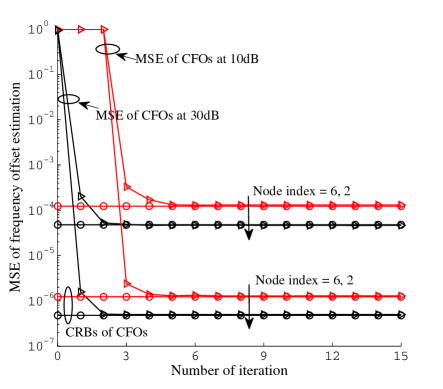
First, consider the network shown in Fig. 2 and each node equipped with two antennas. We employ training with length N=16𝑁16N=16 for relative CFOs estimation and the SNR during training stage in each node is 30dB30dB30\text{dB}. Fig. 4 shows the sum MSE333Sum MSE over the two antennas. of 𝝎isubscript𝝎𝑖\bm{\omega}_{i} for i={3,6,2}𝑖362i=\{3,6,2\} as a function of BP iteration number l𝑙l. It can be seen that the MSEs decrease quickly and touch the corresponding CRBs in only a few iterations.

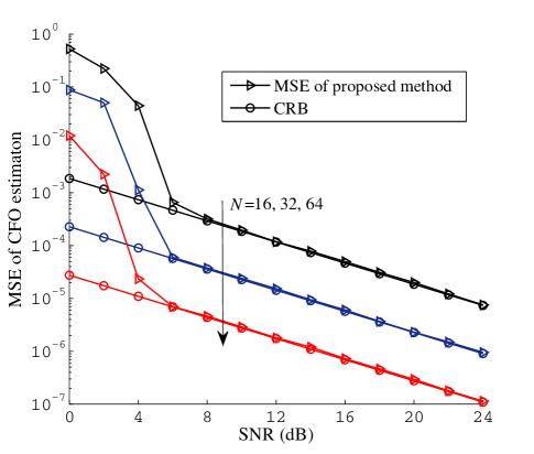
Fig. 5 shows the average sum MSE of {𝝎i}i𝒱subscriptsubscript𝝎𝑖𝑖𝒱\{{\bm{\omega}}_{i}\}_{i\in\mathcal{V}} versus SNRs for different training length N𝑁N. The network is randomly generated within the [0,100]×[0,100]01000100[0,100]\times[0,100] area in each trial, and each node is equipped with 222 antennas. As shown in the figure, the MSEs of proposed distributed algorithm achieve the best performance as the MSEs touch the corresponding CRBs. This verifies Theorem 3. Furthermore, with increasing N𝑁N, 𝑹i,jsubscript𝑹𝑖𝑗\bm{R}_{i,j} touches CRB of the relative CFO 𝑩ϵ{i,j}({ϵk}k=1Nj,{𝒉k}k=1Nj)subscriptsuperscript𝑩𝑖𝑗bold-italic-ϵsuperscriptsubscriptsubscriptbold-italic-ϵ𝑘𝑘1subscript𝑁𝑗superscriptsubscriptsubscript𝒉𝑘𝑘1subscript𝑁𝑗\bm{B}^{\{i,j\}}_{\bm{\epsilon}}(\{{{\bm{\epsilon}}}_{k}\}_{k=1}^{N_{j}},\{{{\bm{h}}}_{k}\}_{k=1}^{N_{j}}) at lower SNR, and thus the estimation MSEs of 𝝎isubscript𝝎𝑖\bm{\omega}_{i} achieves the corresponding CRBs earlier.

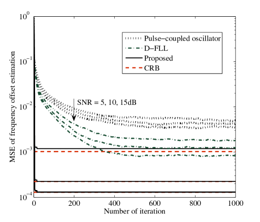
Finally, we compare the performance of the proposed algorithm with that of the D-FLL approach in [29], where CFOs are adjusted to an average common value in each iteration based on consensus principle. The estimation error of consensus method at the lthsuperscript𝑙𝑡l^{th} iteration is measured by the total mean-square deviation of the individual variables from their average, which is

MSEconsensus(l)=1Ki=1K𝔼{𝝁i(l)1Ki=1K𝝁i(l)2}.subscriptsuperscriptMSE𝑙consensus1𝐾superscriptsubscript𝑖1𝐾𝔼superscriptnormsubscriptsuperscript𝝁𝑙𝑖1𝐾superscriptsubscript𝑖1𝐾subscriptsuperscript𝝁𝑙𝑖2\text{MSE}^{(l)}_{\text{consensus}}=\frac{1}{K}\sum_{i=1}^{K}\mathbb{E}\bigg{\{}\big{\|}{\bm{\mu}}^{(l)}_{i}-\frac{1}{K}\sum_{i=1}^{K}{\bm{\mu}}^{(l)}_{i}\big{\|}^{2}\bigg{\}}. (45)

On the other hand, the proposed algorithm estimates the absolute CFO values, therefore, the network estimation MSE at the lthsuperscript𝑙𝑡l^{th} iteration is

MSEBP(l)=1K1i=2K𝔼{𝝁i(l)𝝎i2}.subscriptsuperscriptMSE𝑙BP1𝐾1superscriptsubscript𝑖2𝐾𝔼superscriptnormsubscriptsuperscript𝝁𝑙𝑖subscript𝝎𝑖2\text{MSE}^{(l)}_{\text{BP}}=\frac{1}{K-1}\sum_{i=2}^{K}\mathbb{E}\bigg{\{}\big{\|}{\bm{\mu}}^{(l)}_{i}-\bm{\omega}_{i}\big{\|}^{2}\bigg{\}}. (46)

We consider the 141414 nodes randomly located within the [0,100]×[0,100]01000100[0,100]\times[0,100] area and for fair comparison with D-FLL, each node is equipped with a single antenna. For consensus method, pilots of length 161616 are transmitted by each node in each iteration. However, for the proposed method, 161616 pilots are used only in the relative CFOs estimation at the initial phase. The convergence performance of the two algorithms at different SNRs are shown in Fig. 6. It is apparent that convergence speed of the consensus algorithm decreases with SNRs, and in general takes several hundreds of iterations to converge. For example, at SNR=5SNR5\textrm{SNR}=5dB, around 800800800 iterations is required. Together with the fact that a training of length 161616 is being transmitted by each node in each iteration, this is a huge burden to the network, and also causing long delay in the synchronization process. On the other hand, the proposed method requires only a few iterations of message exchange of two real numbers (mean and variance) to approach the corresponding CRBs.

VI Conclusions

In this paper, a fully distributed CFOs estimation algorithm for cooperative and distributed networks was proposed. The algorithm is based on BP and is easy to be implemented by exchanging limited amount of information between neighboring nodes. Therefore, it has low overhead and is scalable with network size. Furthermore, it was shown analytically that the proposed distributed algorithm converges to the optimal solution with estimation MSE coincides with the centralized CRB asymptotically regardless of the network topology. Simulation results showed that the MSE of the proposed method touches the CRB within only a few iterations.

References

  • [1] H. Meyr, M. Moeneclaey, and S. A. Fechtel, Digital Communication Receivers: Synchronization, Channel Estimation, and Signal Processing. Wiley-InterScience, John Wiley & Sons, Inc., 1997.
  • [2] T. Pollet, M. V. Bladel, and M. Moeneclaey, “BER sensitivity of OFDM systems to carrier frequency offset and Wiener phase noise,” IEEE Trans. Commun., vol. 43, pp. 191–193, Feb./Mar./Apr. 1995.
  • [3] H. Steendam and M. Moeneclaey, “Synchronization sensitivity of multicarrier systems,” European Commun., ETT special issue on multi-carrier spread spectrum, vol. 52, no. 5, pp. 834-844, May 2004.
  • [4] V. K. V. Gottumukkala and H. Minn, “Capacity analysis and pilotdata power allocation for MIMO-OFDM with transmitter and receiver IQ imbalances and residual carrier frequency offset,” IEEE Trans. Veh. Technol., vol. 61, no. 2, pp. 553-565, Feb. 2012.
  • [5] I.-H. Wang and D. N. C. Tse, “Interference mitigation through limited receiver cooperation, IEEE Trans. Inf. Theory., vol. 57, no. 5, pp. 2913-2940, May 2011.
  • [6] V. Havary-Nassab, S. Shahbazpanahi, A. Grami, and Z. Q. Luo, “Distributed beamforming for relay networks based on second-order statistics of the channel state information,” IEEE Trans. Signal Process., vol. 56, no. 9, pp. 4306-4316, Sep. 2008.
  • [7] L. Dong, P. Petropulu, and H. V. Poor, “A Cross-Layer Approach to Collaborative Beamforming for Wireless Ad Hoc Networks,” IEEE Trans. Signal Proc., vol. 56, July 2008, pp. 2981-93.
  • [8] A. D. Wyner, “Shannon-theoretic approach to a Gaussian cellular multiple-access channel,” IEEE Trans. Inf. Theory, vol. 40, no. 6, pp. 1713-1727, Nov. 1994.
  • [9] R. Irmer, H. Droste, P. Marsch, M. Grieger, G. Fettweis, S. Brueck, H.-P. Mayer, L. Thiele, and V. Jungnickel, “Coordinated multipoint: Concepts, performance, and field trial results,” IEEE Commun. Mag., vol. 49, no. 2, pp. 102-111, Feb. 2011.
  • [10] D. Gesbert, S. Hanly, H. Huang, S. Shamai, O. Simeone, and W. Yu, “Multi-cell MIMO cooperative networks: a new look at interference,” IEEE J. Select. Areas Commun., vol. 28, no. 9, pp. 1380-1408, Dec. 2010.
  • [11] J. G. Andrews, H. Claussen, M. Dohler, S. Rangan, and M. C. Reed, “Femtocells: Past, present, and future,” IEEE J. Select. Areas Commun., vol. 30, no. 3, pp. 497 – 508, April 2012.
  • [12] J. G. Andrews “The Seven Ways HetNets are a Paradigm Shift”, to appear in IEEE Comm. Mag., Mar. 2013.
  • [13] F. Pantisano, M. Bennis, W. Saad, and M. Debbah, “Spectrum Leasing as an Incentive towards Uplink Macrocell and Femtocell Cooperation,” IEEE J. Select. Areas Commun., vol. 30, no. 3, 617 – 630, April 2012
  • [14] M. Morelli and U. Mengalli, “Carrier-frequency estimation for transmissions over selective channels,” IEEE Trans. Commun., vol. 48, pp. 1580–1589, Sep. 2000.
  • [15] L. Sanguinetti, M. Morelli, and G. Imbarlina, “An EM-based frequency offset estimator for OFDM systems with unknown interference,” IEEE Trans. Wireless Commun., vol. 8, no. 9, pp. 4470–4475, Sep. 2009.
  • [16] M. Ghogho and A. Swami, “Training design for multipath channel and frequency-offset estimation in MIMO systems,” IEEE Trans. Signal Process., vol. 54, no. 10, pp. 3957–3965, Oct. 2006.
  • [17] O. Besson and P. Stoica, “On parameter estimation of MIMO at fading channels with frequency offsets,” IEEE Trans. Signal Process., vol. 51, no. 3, pp. 602–613, Mar. 2003
  • [18] M. O. Pun, M. Morelli, and C.-C. J. Kuo, “Maximum-likelihood synchronization and channel estimation for OFDMA uplink transmissions,” IEEE Trans. Commun., vol. 54, no. 4, pp. 726–736, Apr. 2006.
  • [19] T. Pham, A. Nallanathan, and Y. Liang, “Joint channel and frequency offset estimation in distributed MIMO flat-fading channels,” IEEE Trans. Wireless Commun., vol. 7, no. 2, pp. 648–656, Feb. 2008
  • [20] J. Chen, Y.-C. Wu, S. Ma, and T.-S. Ng, “Joint CFO and channel estimation for multiuser MIMO-OFDM systems with optimal training sequences,” IEEE Trans. Signal Process., vol. 56, no. 8, pp. 4008-4019, Aug. 2008.
  • [21] H. Mehrpouyan and S. D. Blostein, “Bounds and algorithms for multiple frequency offset estimation in cooperative networks,” IEEE Trans. Wireless Commun., vol. 10, no. 4, pp. 1300–1311, Apr. 2011.
  • [22] H. G. Jeon, K. S. Kim, and E. Serpedin, “An efficient blind deterministic frequency offset estimator for OFDM systesm,” IEEE Trans on Communications., vol. 59, no. 4, Apr. 2011.
  • [23] F. F. Gao, T. Cui, A. Nallanathan, and C. Tellambura, “Maximum likelihood based estimation of frequency and phase offset in DCT OFDM systems under non-circular transmissions: Algorithms, analysis and comparisons,” IEEE Trans on Communications., vol. 56, no. 9, pp. 1425–1429, Sep. 2008.
  • [24] P. A. Parker, P. Mitran, D. W. Bliss, and V. Tarokh, “On bounds and algorithms for frequency synchronization for collaborative communication systems,” IEEE Trans. Signal Process., vol. 56, no. 8, pp. 3742-3752, Aug. 2008.
  • [25] B. Zarikoff and J. Cavers, “Coordinated multi-cell systems: Carrier frequency offset estimation and correction,” IEEE Trans. Select. Areas Commun., vol. 28, no. 9, pp. 1490–1501, Dec. 2010
  • [26] R. Mudumbai, G. Barriac, and U. Madhow, “On the feasibility of distributed beamforming in wireless networks,” IEEE Trans. Wireless Commun., vol. 6, no. 5, pp. 1754–1763, May 2007.
  • [27] D. R. Brown III and H. V. Poor. “Time-Slotted Round-Trip Carrier Synchronization for Distributed Beamforming,” IEEE Trans. Signal Process., vol. 56, no. 11, pp. 5630-5643, November 2008.
  • [28] R. Preuss and D. R. Brown III. “Two-Way Synchronization for Coordinated Multicell Retrodirective Downlink Beamforming,” IEEE Trans. Signal Process.,vol. 59, no. 11, 5415-5427, November 2011.
  • [29] N. Varanese, U. Spagnolini, Y. Bar-Ness, “Distributed frequency-looked loops for wireless networks,” IEEE Trans on Communications., vol.59, n.12, pp. 3440-3451, Dec. 2011
  • [30] S. M. Kay, Fundamentals of Statistical Signal Processing Estimation Theory, Upper Saddle River, NJ: Prentice-Hall, 1993.
  • [31] P. Stoica and O. Besson, “Training sequence design for frequency offset and frequency-selective channel estimation,” IEEE Trans. Commun, vol. 51, no. 11, pp. 1910-1917, Nov. 2003.
  • [32] L. L. He, S. D. Ma, Y. C. Wu, and T. S. Ng, “Semiblind iterative data detection for OFDM systems with CFO and doubly selective channels,” IEEE Trans. on Commun., vol. 58, no. 12, pp. 3491-3499, Dec. 2010.
  • [33] E. Simon, L. Ros, H. Hijazi, and M. Ghogho, Joint carrier frequency offset and channel estimation for OFDM systems via the EM algorithm in the presence of very high mobility,” IEEE Trans. Signal Process., vol. 60, no. 2, pp. 754–765, Feb. 2012
  • [34] F. R. Kschischang, B. J. Frey, and H.-A. Loeliger, “Factor graphs and the sum-product algorithm,” IEEE Trans. Inf. Theory, vol. 47, no. 2, pp. 498-519, Feb. 2001.
  • [35] Y. Weiss and W. T. Freeman, “Correctness of belief propagation in Gaussian graphical models of arbitrary topology,” Neural Computation, vol, 13, no. 10, pp. 2173-2200, 2001.
  • [36] D. M. Malioutov, J. K. Johnson, and A. S. Willsky, “Walk-sums and belief propagation in Gaussian graphical models,” Journal of Machine Learning Research, vol, 7, Oct. 2006.
  • [37] M. Leng and Y.-C. Wu, “Distributed clock synchronization for wireless sensor networks using belief propagation,” IEEE Trans. Signal Process., vol. 59, no. 11, pp. 5404–5414, Nov. 2011.
  • [38] A. Papoulis and S. U. Pillai, Random Variables and Stochastic Processes, 4th ed. New York: McGraw-Hill, 2002.
  • [39] S. Puntanen, G. Styan, and J. Isotalo, Matrix Tricks for Linear Statistical Models Our Personal Top Twenty, Springer, 2011.
  • [40] A. M. Sarhan, N. M. EI-Shazly, and E. M. Shehata, On the existence of extremal positive defnite solutions of the nonlinear matrix equation 𝑿r+i=1m𝑨i𝑿δi𝑨i=𝑰superscript𝑿𝑟superscriptsubscript𝑖1𝑚subscriptsuperscript𝑨𝑖superscript𝑿subscript𝛿𝑖subscript𝑨𝑖𝑰\bm{X}^{r}+\sum_{i=1}^{m}{\bm{A}}^{\ast}_{i}{\bm{X}}^{\delta_{i}}{\bm{A}}_{i}=\bm{I},” Mathematical and Computer Modelling, vol. 51, no. 9- 10, 2010.
  • [41] R. A. Horn and C. R. Johnson, Matrix Analysis. Cambridge, U.K.: Cambridge Univ. Press, 1985.
  • [42] J. W. Demmel Applied Numerical Linear Algebra. SIAM, 1997.
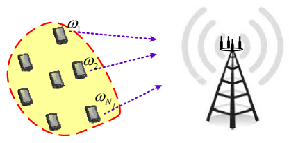
    

Refer to caption
(a) Distributed beamforming networks
Refer to caption
(b) Multi-cell cooperative networks
Refer to caption
(c) A 3-tier HetNet with macro, pico and femto cells.
Figure 1: Scenarios that need network-wide frequency synchronization
Refer to caption
Figure 2: An example of arbitrary network topology with 14 nodes.
Refer to caption
Figure 3: The factor graph representation of the network in Fig. 2.
Refer to caption
Figure 4: Convergence performance of the proposed algorithm at different nodes.
Refer to caption
Figure 5: MSE of CFOs {𝝎i}i𝒱subscriptsubscript𝝎𝑖𝑖𝒱\{{\bm{\omega}}_{i}\}_{i\in\mathcal{V}} averaged over the whole network with respect to SNRs.
Refer to caption
Figure 6: Convergence of the proposed method and consensus method in [29] in single antenna case.