Scalable Bayesian Modeling, Monitoring and
Analysis of Dynamic Network Flow Data

Abstract

Traffic flow count data in networks arise in many applications, such as automobile or aviation transportation, certain directed social network contexts, and internet studies. Using an example of internet browser traffic flow through domains of an international news website, we present Bayesian analyses of two linked classes of models which, in tandem, allow fast, scalable and interpretable Bayesian inference. We first develop flexible state-space models for streaming count data, able to adaptively characterize and quantify network dynamics effectively and efficiently in real-time. We then use these efficiently implemented models as emulators of more structured, time-varying gravity models that allow closer and formal dissection of network dynamics. This yields interpretable inferences on traffic flow characteristics, and on dynamics in interactions among network nodes. Bayesian model monitoring theory defines a strategy for sequential model assessment and adaptation in cases of signaled departures of network flow data from model-based predictions. Exploratory and sequential monitoring analyses of evolving traffic on a defined network of web domains in e-commerce demonstrate the utility of this coupled Bayesian emulation approach to analysis of streaming network count data.

KEY WORDS: Bayesian model emulation, Decouple/Recouple, Dynamic network flow model, Dynamic gravity model, Monitoring and anomaly detection

1 INTRODUCTION

Increasing access to streaming data on dynamic networks drives interest in formal models to quantify stochasticity and structure of latent processes underlying observable data streams. Modeling interests are coupled with concerns to monitor and adapt to changing patterns, and to signal and highlight dynamics that may reflect interesting departures from the norm. Key challenges are real-time/sequential analysis and scalability: interest lies in relevant statistical models whose analyses are inherently sequential in time, as well as computationally efficient and scalable with network size and sampling rates. Relevant models should also define sound statistical methods for monitoring and short-term prediction, and elucidate the complexities and dynamics in network structure in both single sample inference and multi-sample comparisons across contexts.

We contribute to this area with modeling and methodological developments coupled with a motivating applied study of internet traffic in e-commerce. Consistent with the primary applied goals outlined above, the main contributions of this work are as follows.

• A flexible and customized statistical modeling framework for: (i) characterizing patterns of temporal variation in network flows at the levels of nodes and pairs of nodes; (ii) model-based exploratory data analyses of network flows within and across contexts; and (iii) the ability to scale to large networks.

• Use of these flexible, efficient models as Bayesian emulators of more structured network flow models. This yields computationally efficient dissection of the dynamics to evaluate node-specific and dependence/interaction effects across nodes in a structured model context where analysis is otherwise computationally challenging in more than small networks.

• Formal Bayesian model assessment methodology for sequential monitoring of flow patterns with the ability to signal departures from predictions in real-time and allow informed interventions as a response, and in a scalable framework.

• Development and validation of the above in exploratory and monitoring analyses of data from the motivating application; here the observations are streaming counts of visitors in a set of defined web domains (collections of webpages) in a structurally well-defined but dynamic/evolving website. This includes evaluation of node-specific and node-pair interactions in the flow dynamics within the network over a given time period, comparisons across time periods and across days, and analyses utilizing Bayesian monitoring and adaptation to respond to departures from predicted flow patterns.

Following a discussion of the motivating applied setting, network and data in Section 2, we develop our class of Bayesian dynamic flow models (BDFMs) in Section 3. BDFMs are flexible univariate dynamic models for series of counts representing flows into the network and between within-network node pairs. These (non-stationary and non-normal) state-space models for streaming count data rely on discrete-time gamma processes historically used in volatility modeling, and that have very recently become of interest as flexible smoothing and short-term predictive models for space-time processes underlying count data. Our use of these models for within-network flows is novel and involves methodological extension to adapt and customize them to provide suitable univariate emulators of the underlying, inherent dynamic multinomial structures governing flows at each time point. This use of sets of decoupled univariate models that are then recoupled to define the actual multinomial probability processes is: (a) explicitly designed to be computationally efficient in on-line data analysis, scaling quadratically in the number of network nodes and enabling distributed implementation for streaming data on large networks; (b) allows for diverse patterns in the dynamics of flow rates that a time-varying Dirichlet-multinomial model simply annot; and (c) relates to the recent development of conceptually similar (decouple/recouple) approaches that have advanced multivariate dynamic modeling in conditionally normal contexts (Gruber and West 2016a; Zhao et al. 2016; Gruber and West 2016b). Section 3.4 discusses some aspects and summaries of exploratory analysis of the network flow data from a defined MaxPoint network of the Fox News website. This highlights the use of customized BDFMs, with one focus on exploring aspects of flow dynamics on the network across the same time periods on different days. The supporting appendix material gives additional technical details and discussion.

Section 4 introduces a class of more highly structured dynamic gravity models (DGMs) for network flows. These are non-normal, log-linear random-effects models with time-varying parameters for flow rate contributions of origin nodes, destination nodes and origin-destination interaction effects. Our DGMs extend prior work with static gravity models (e.g. West 1994; Sen and Smith 1995; Congdon 2000; Jandarov et al. 2014) to the time-varying parameter context, defining a class of models able to represent complicated patterns of dependency structure, and their temporal variations, across nodes. Importantly, we show that the flexible and computationally simple BDFM framework can be mapped one:one to that of the DGM. This underlies one further novel contribution of this work: the use of the fast, efficient BDFMs as emulators of DGMs. This is key from the viewpoint of scalability; fitting gravity models, even without time-varying parameters, is a challenging issue in more than modest dimensional networks, and simply infeasible in any realistic dynamic extension appropriate for scalable, on-line analysis of streaming network flow data. Further, we avoid the challenging approach of defining and parametrizing time-evolution models for DGMs directly, adopting the implicit structures induced in the mapping from BDFMs where model specification and fitting is relatively facile. Example results and highlights from the Bayesian emulation analysis of DGMs for the MaxPoint Fox News study appear in Section 4.3.

Section 5 develops methods of formal, sequential Bayesian model monitoring and adaptation (automatic intervention) for BDFMs. The aim here is to build into the fast, decoupled analysis an ability to efficiently evaluate incoming flows against model predictions so as to signal data– at the level of individual nodes and node-pairs– that appear discrepant, and that may signal outliers or changes in flow trends/rates beyond the norm. In addition to signaling such events and thus providing opportunity for direct intervention, we couple monitoring with the use of automatic intervention to allow the model to appropriately adapt to data at the next few time points. This Bayesian testing/adaptation strategy builds on core theory underlying its use in time series forecasting contexts with dynamic linear models (West 1986; West and Harrison 1986; Harrison and West 1987; West and Harrison 1989a; see also chapter 11 of West and Harrison 1997). Some of the novelty here is in the use of these ideas in non-linear, non-normal dynamic models for count data– our class of BDFMs. Importantly, monitoring is applied in parallel across nodes and node-pairs, so is also scalable with network size. Some departures from normal variation in patterns of flow may be related across nodes, and the approach has an ability to explore and evaluate this both within the BDFM model context and then following the map to more structured DGMs that directly reflect interaction effects. Application to the Fox News network data highlights some aspects of the use of this in connection with selected network nodes. Summary comments conclude the paper in Section 6, and additional supporting material is given in the Appendix.

2 Web-Domain Network Flows

2.1   Context and Data

Our context is traffic flow among domains (defined sets of pages) of the Fox News website. Domains include the Homepage and several categories of news and consumer content– such as Politics, Entertainment, Travel, Science, etc.– as defined by Fox News. While the domain structure is persistent, the nature of webpage definition and content within a domain is dynamic; content changes on a daily basis (updated at midnight) but also more rapidly when noteworthy events occur. MaxPoint places ads on pages in these Fox News domains, and thus can track flows of anonymized users as they move through its pages. While some users can be tracked individually, this is not the norm, and we focus in this paper on aggregated flow counts, not the trajectories of individuals.

On-line advertisers are interested in a host of statistical issues related to traffic flow and domain content. The field has become quite sophisticated, employing complex recommender systems (Koren et al. 2009), sentiment analysis (Pang and Lee 2008), text mining (Soriano et al. 2013), and other methods (Agarwal et al. 2010; Taddy 2013). However, basic questions of understanding and characterizing traffic across domains have not received the attention they require. In particular, there is commercial value in identifying how the popularity of a site changes on short time scales, and how sites interact with respect to traffic. As example, our data showed a morning-after spike in traffic to the Entertainment domain following the Grammy awards, which would have been an opportunity to market concert tickets; unusual interactions in flows between Science and Health may reflect new medical findings that might incline people to purchase gym memberships; increased flow rates from Homepage to Science that contradict the general stable or somewhat decreasing trends of overall traffic may indicate specific opportunities to target scientific product consumers.

As pages within a domain are updated, questions arise as to whether browsing traffic patterns change as a result. To address this statistically, we need to understand stochastic variation in past browser traffic so that comparisons can be made of incoming traffic streams against recent statistical “norms”, and significant deviations from short-term predictions based on current dynamic patterns can be identified. Companies that have flow models which enable them to predict how traffic will change as content changes, that are able to sensitively characterize and monitor patterns of change in interactions as well as overall rates, and that can signal anomalous changes to provide opportunities for intervention and actions, will be advantaged. They can recognize opportunities more quickly, and– for example– may then adapt bidding strategies for relevant keywords to be dynamically calibrated to expected revenue.

2.2   Data

The data set contains Fox News website visit data during 09:00–10:00am and 01:00–02:00pm EST on each of six days, February 23rd-24th, March 2nd-3rd and 9th-10th, 2015. These days are Mondays or Tuesdays. Since the Fox News website structure changes often, with new pages being added and old pages being archived, the analysis aggregates webpages into groups specified by the host domain www.foxnews.com, and the set of first url paths after the host domain, including examples such as e.g. www.foxnews.com/politics/* and www.foxnews.com/US/*. These classify all pages into 22 domains: Homepage, Politics, US, Opinion, Entertainment, Technology, Science, Health, Travel, Leisure, World News, Sports, Shows, Weather, Category, Latino, Story, On-Air, Video, National News, Magazine, and Other.

The data set includes anonymized visitors from nearly every time zone on the planet. In order to study time-of-day effects, such as, say, a tendency to browse news in the morning and entertainment in the afternoon, it is necessary to stratify by time zone. Here we focus on users in the Eastern North America time zone; those are the most numerous, and the two time windows used in this study were chosen with the expectation that different browsing patterns might occur at those times.

Aggregate data give time series of counts in half-minute intervals, i.e., $120$ time points of domain occupancy, flows from each domain, and flows into each domain. In each half minute interval, if the record shows the same user in two or more domains, then each of her/his moves is counted in the flow data into each of these domains. If the user refreshes the same page multiple times spanning more than one time interval, then s/he is counted as simply staying in that domain; this can be done as the web browsing tool performs automatic refresh. Importantly, if a user stays in the same domain for more than five minutes, s/he is declared as no longer active and counted as leaving the Fox News site. If such a user later appears in one domain, s/he counts as inflow from outside the Fox News site. Finally, we cannot track user information either before or after the one-hour observation window; we thus restrict attention to the period 09:05–09:55am and 01:05–01:55pm, consisting of uncensored flows, using the first 5 minutes of data informally to define priors. Thus the series runs from $t=1{:}T$ with $T=110$ in each time period.

Aggregation at half-minute intervals reflects a balance of interests in fine-time scale modeling against information content of data with low flow rates. For domain pairs with low flow rates it is sometimes too low, leading to excessive volatility in the BDFM and noisy parameter estimates in the DGM. No single window is good for all node pairs at all times, but preliminary exploration found this to be a good compromise. The decision that a user is inactive after five minutes is based on previous research on how users access on-line articles. Few people read more than the first paragraph of a news story, and at the times of day for which data were collected, interruptions are likely. Investigations of on-line session length have focused on dynamics of search engine use (e.g. Silverstein et al. 1999; Qiu et al. 2005, and references therein) in settings where the full breadth of user browsing behavior is visible. Using additional context such as change in search engine query topic, these studies have derived average user session lengths between 5–60minutes (Jansen et al. 2007). We employed a session length limit on the lower end of this spectrum due to the fact that a user is likely to only spend a fraction of a larger total browsing session on Fox News.

2.3   Network Structure and Notation

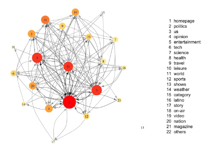
Referring to sites external to the Fox News website as node 0, we have $23$ network nodes; the $I=22$ actual domains and “External”, indexed as $i=0{:}I.$ At each time $t=1{:}T,$ define $x_{ijt}$ as the flow count from node $i$ to $j$, including the inflows $x_{0it}$ and outflows $x_{i0t}$ relative to the External domain. Also, denote the number of occupants of node $i$ at the end of the $t$ period by $n_{it}$– a random quantity at the start of the period, but then known and given by the sum of inflows minus outflows at the end of the period. Figure 2 provides a visualization of data at the first time interval, and the schematic in Figure 2 reflects our notation.

If $\phi>0$ has a gamma distribution with shape $r$ and scale $1/c$, we write $\phi\sim Ga(r,c)$, noting that $E(\phi)=r/c$ and $V(\phi)=r/c^{2}.$ If $\eta\in(0,1)$ has a beta distribution with p.d.f. proportional to $\eta^{a-1}(1-\eta)^{b-1}$ for $a>0,b>0,$ we write $\eta\sim Be(a,b).$ If the $n-$vector of counts $z$ has a multinomial distribution with total counts $n$ and probability vector $\theta,$ we write $z\sim Mn(n,\theta).$ For any series of random quantities $z_{t}$ over $t=0,1,\ldots,$ we use the succinct notation $x_{h:k}=\{x_{h},x_{h+1},\ldots,x_{k}\}$ for any indices $h\leq k.$

Figure 1: A snapshot of counts and flows on the Fox News network at time time $t=1$ (09:05.30 on February 23rd 2015). The circular numbered nodes represent the domains, with diameters (and, in the online paper, color) proportional to occupancy $n_{it}$ for node $i$ at this time point $t.$ Each arrow $i\rightarrow j$ has width proportional to flow $x_{ijt}.$

Figure 2: Network schematic and notation for flows at time $t$.

3 Fast, Flexible Dynamic Flow Models

3.1   Background: Discrete-Time Volatility Models for Poisson Rates

BDFMs are based on gamma-beta random walks that have been key to stochastic volatility modeling for more than 30 years (West and Harrison 1989b, 1997, Section 10.8). Based initially on Bayesian discount concepts related to exponential smoothing for volatilities (Ameen and Harrison 1985; Harrison and West 1987; Quintana and West 1987) and with “steady” evolutions in non-Gaussian dynamic models (Smith 1979), these gamma-beta discount models yield closed form Bayesian analyses. They have seen some– though limited– use as models for rates underling time series of conditionally Poisson counts (Harvey and Fernandes 1989; Brandt et al. 2000), which is a starting point here. We extend the applicability of the basic model in a number of ways, with novel model forms customized to the network flow context and that define flexible models for conditional multinomial data with time-varying probabilities that go beyond prior use. We also heavily utilize full Bayesian posterior simulation of posteriors for latent rate processes, extending the use from the normal/linear dynamic volatility modeling context (Prado and West 2010, Chapter 4).

The essentials of gamma-beta discount models follow; see Appendix A for further details and discussion. In generic notation, suppose that $x_{t}$ is a time series with $x_{t}|\phi_{t}\sim Poi(m_{t}\phi_{t})$ conditionally independently over $t=1,2,\ldots.$ Here $\phi_{t}$ is a latent level process and $m_{t}$ a scaling factor known at time $t$. The $\phi_{t}$ process evolves via the Markov model

$$\phi_{t}=\phi_{t-1}\eta_{t}/\delta_{t},\qquad\eta_{t}\sim Be(\delta_{t}r_{t},(1-\delta_{t})r_{t}),\qquad\eta_{t}\perp\!\!\!\perp\eta_{s},\phi_{s},\,\,s<t,$$ (1)

where $\delta_{t}\in(0,1)$ is a specified discount factor and $r_{t}$ is a known function of $t,x_{0{:}t-1},$ and independent innovations $\eta_{t}/\delta_{t}$ drive the evolution. The beta distributions imply: (i) $E(\phi_{t}|\phi_{t-1})=\phi_{t-1},$ hence this is a multiplicative random walk model, or “steady” evolution; (ii) a lower value of $\delta_{t}$ leads to a more diffuse distribution for $\eta_{t}/\delta_{t}$, and hence increased uncertainty about $\phi_{t}$ and adaptability to changing rates over time; a value closer to one indicates a steady, stable evolution.

The model is structured to ensure full conjugacy in the forward filtering/Bayesian sequential learning over time, and in retrospective analysis. This is reflected in some key summaries, as follows and with further details in Appendix A. Here $x_{0}$ is a synthetic notation for initial information.

• Forward Filtering (FF): At any time $t,$ both the prior $p(\phi_{t}|x_{0{:}t-1})$ and the posterior $p(\phi_{t}|x_{0{:}t})$ for the “current” latent level are gamma distributions, with trivially computed parameters that are updated as $t$ evolves

• One-Step Forecasts: The one-step ahead forecast distribution made at time $t-1$ to predict time $t$ is generalized negative binomial with p.d.f. in eqn. (7). On observing $x_{t},$ the p.d.f. is trivially evaluated to feed into computation of model marginal likelihoods (MMLs, as in Appendix) for assessment.

• Backward Sampling: At end time $T,$ recursive simulation generates time trajectories $\phi_{0{:}T}$ of the rate process under its full posterior $p(\phi_{0{:}T}|x_{0{:}T}).$ The computations are trivial, as detailed in Section A.3.

The model can be defined by any sequence of specified discount factors $\delta_{t}.$ A constant value over time defines a global smoothing rate; values closer to 1 constrain the stochastic innovation and hence the change from $\phi_{t-1}$ to $\phi_{t}$; smaller discount factor values lead to greater random changes in these Poisson levels. Intervention to specify smaller discount factors at some time points, to reflect or anticipate higher levels of dynamic variation at those times, are sometimes relevant. In our network flow models below, we customize the specification of the sequence of discount factor to address issues that arise in cases of low flow levels. That extension of discount-based modeling defines the $\delta_{t}$ as time-varying functions of an underlying base discount rate, and the latter are then evaluated using MML measures.

This model provides the basis for flows into network nodes; we adapt and generalize it to define components of flexible multinomial dynamic models for flows between nodes in a network.

3.2   Network Inflows: Poisson Dynamic Models

With notation for inflows as in Figure 2, we adopt the general model of Section 3.1 by adding suffices $i$ for network nodes and setting the Poisson mean scaling factors to 1. We now customize this model via specification of discount factor sequences. At any node $i,$ the time $t$ inflow to node $i$ is $x_{0it}\sim Poi(\phi_{it})$ independently across nodes $i=1{:}I,$ and the latent levels $\phi_{it}$ follow node-specific gamma-beta discount models with discount factor $\delta_{it}$ at time $t.$ The time $t\to t+1$ update/evolve steps are: (i) the time $t$ prior $\phi_{it}|x_{0i,0{:}t-1}\sim Ga(\delta_{it}r_{i,t-1},\delta_{it}c_{i,t-1})$ updates to the posterior $\phi_{it}|x_{0i,0{:}t}\sim Ga(r_{it},c_{it})$ with $r_{it}=\delta_{it}r_{i,t-1}+x_{0it}$ and $c_{it}=\delta_{it}c_{i,t-1}+1.$ This then evolves to the time $t+1$ prior $\phi_{i,t+}|x_{0i,0{:}t}\sim Ga(\delta_{i,t+1}r_{i,t},\delta_{i,t+1}c_{it})$, and so on. Specifying discount factors $\delta_{it}$ relates to the information content of gamma distributions as measured by the shape parameters $r_{i*}$; evolution each time point reduces this by discount factor, the latter representing a per-time-step decay of information induced by the stochastic evolution. Our specification of discount rates is motivated by the following considerations. First, baseline levels of variation on $\phi_{it}$ are likely to be node specific, so that each node should have its own baseline discount rate to be assessed in data analysis. Second, in cases of zero flow rates for a period of time, $r_{it}$ is continually discounted and shrinks towards 0 while $c_{it}$ is incremented by 1 at each update step. That is, discounting is not balanced by the prior-posterior update and the generates more and more diffuse posteriors favoring lower and lower $\phi_{it}.$ Ideally, the posterior and prior should be very similar in cases of 0 flows, and we address this with the specification $\delta_{it}=d_{i}+(1-d_{i})\exp(-kr_{i,t-1})$ at each $i,t,$ where $d_{i}$ is a constant baseline discount factor for node $i$ and $k>0$ a specified constant. The aim is that $\delta_{it}$ be close to the baseline unless information content is very low; this our applied studies take $k=1$ (so that $\delta_{it}$ be close to– within 10% of– the baseline when $r_{i,t-1}>2$). Then in cases of high information content, the effective $\delta_{it}$ is close to $d_{i};$ otherwise, $\delta_{it}$ will be closer to 1 in cases of low information content, so appropriately limiting the decay of information in such cases.

Node-specific MML measures that feed into model assessment to aid in selection of the baseline discount factors $d_{i}.$ These measures of short-term predictive fit of the models can also be monitored sequentially over time for on-line tracking of model performance. This ability to flag anomalous data at one node or any subset of nodes is key to commercial application of the analysis, since that corresponds to new opportunities or new threats (e.g., offer concert tickets after the Grammy Awards, but not on David Bowie’s obituary). This view on anomaly detection is extended below, in Section 5, using Bayesian model monitoring concepts. One aspect of this is the ability to signal a need to temporarily reduce the value of the discount factor for a node at a time of degradation of predictive performance that may relate to changes in $\phi_{it}$ that are larger than the “standard” baseline discount factor value $d_{i}$ determines.

3.3   Transitions from Network Nodes: Multinomial Dynamic Models

Transitions from any node $i$ at time $t$ are inherently multinomial with time-varying transition probabilities. To build flexible and scalable models for dynamics and dependencies in transition probability vectors is a challenge, with computational issues for even simple models quickly dominating. Novel models here adapt and extend the univariate Poisson/gamma-beta random walk models to enable flexibility in modeling node-pair specific effects as they vary over time as well as scalability.

Considering flows from node $i$ to node $j$ at time $t,$ and using notation as in Figure 2, the core model is $x_{i,0{:}I,t}\sim Mn(n_{i,t-1},\theta_{i,0{:}I,t})$ where the current node $i$ occupancy level is $n_{i,t-1},$ and $\theta_{i,0{:}I,t}$ is the $(I+1)$-vector of transition probabilities $\theta_{ijt}$ (including the “external” node– i.e., leaving the Fox News network– at $j=0).$ We structure decoupled BDFMs in terms of positive flow rates $\phi_{ijt}$ underlying each $x_{ijt}.$ Specifically,

$$x_{ijt}\sim Poi(m_{it}\phi_{ijt}),\qquad m_{it}=n_{i,t-1}/n_{i,t-2},$$ (2)

independently, with independent gamma-beta evolutions for each latent level $\phi_{ijt}.$ These BDFMs for each node pair can be customized with node-pair specific discount factors, allowing greater or lesser degrees of variation by node pair. The set of models for elements of $\phi_{i,0{:}I,t}$ implies a dynamic model for the vector of transition probabilities $\theta_{i,0{:}I,t}$ having elements $\theta_{ijt}=\phi_{ijt}/\sum_{j=0{:}I}\phi_{ijt}.$ Independence across nodes enables scaling, as the analyses can then be decoupled and run in parallel for the $\phi_{ijt}$ and then recoupled to infer the $\theta_{ijt}.$ Dependencies in patterns of changes in the $\phi_{ijt}$ are recovered in evaluating the posterior distributions and, as in Section 4, in using this set of models to emulate gravity models that explicitly characterize interdependencies.

A key and critical component of the model is the definition of the scaling factors $m_{it}$ in eqn. (2). In decoupling the multinomial flows from node $i$ into parallel Poisson models for nodes $i\to j$ the inherent dependency on total occupancy of node $i$ is lost. We restore this in using this specific definition of scaling factors to explicitly correct for occupancy changes. This recognizes that the decoupled, scaled models are not predictive of overall occupancy– rather, they are decoupled, tractable models that are relevant to tracking and short-term prediction of relative occupancy levels through the implied multinomial probabilities. The relevance of this scaling factor is most evident in cases of major changes in occupancy, when an abrupt increase in node $i$ occupancy $n_{i,t-1}$ at time $t-1$ relative to its prior value $n_{i,t-2}$ will lead to increased flows to other nodes at time $t$ even if the underlying transition probabilities $\theta_{i,0{:}I,t}$ are essentially constant. In such a case, the scaling factor will encourage the appropriate view that the $\phi_{ijt}$ are stable. Then, inferences on the $\phi_{ijt}$ directly yield inferences on the transition probabilities of interest: theoretically, the conditional multinomial probabilities are simply not impacted by the scaling factors, i.e.,

$$\theta_{ijt}=m_{it}\phi_{ijt}/\sum_{j=0{:}I}m_{it}\phi_{ijt}=\phi_{ijt}/\sum_{j=0{:}I}\phi_{ijt}.$$

The theory and analysis details of Section 3.1 and Appendix A now apply with data and latent flow levels indexed by origin node $i$ and destination node $j.$ As with inflow models, we have flexibility to choose discount factors specific to context. Following the discussion of Section 3.2, we specify $\delta_{ijt}=d_{ij}+(1-d_{ij})\exp(-kr_{ij,t-1})$ at each $i,j,t,$ where $d_{ij}$ is a constant baseline discount factor for node pair $i,j$ and $k>0$ a specified constant. Again this is later overlaid with intervention to adjust discount factor values as needed, based on sequential monitoring of flow patterns and using the MML measures– now of course for each node pair– as one formal guide to model adequacy.

In sequential analysis of transitions, the node-pair specific models generate full joint predictions one-step ahead (or more, if desired) for the theoretically exact set of multivariate flow vectors $x_{i,0{:}I,t}$ across all nodes. The one-step forecast distribution does not have an analytic closed form, but is trivially simulated to define forecasts. That is: (i) simulate directly from each of the gamma-beta evolutions for the $\phi_{ijt};$ (ii) transform sampled values to the conditional multinomial probabilities $\phi_{ijt}$; then (iii) sample the multinomial $x_{i,0{:}I,t}\sim Mn(n_{i,t-1},\theta_{i,0{:}I,t})$ at these parameter values. Similarly, for both on-line and retrospective inference about transition probabilities, samples from posteriors for the $\phi_{ijt}$ again simply transform to the required probability scale.

3.4   Aspects of BDFM Analysis of Fox News Data

The analysis was applied separately to data from each of the six days. We focus on the am period of February 23rd 2015 for initial summaries, and then make some comparisons across days. Priors for the inflow rates are $\phi_{i0}|x_{0i0}\sim Ga(r_{i0},c_{i0})$ with $c_{i0}=1$ and $r_{i0}=c_{i0}z_{i}$ where $z_{i}$ is from inflows in the 5minutes prior to the start of model analysis at $t=1.$ The priors for the node-node flows are, similarly, $\phi_{ij0}|x_{0ij0}\sim Ga(r_{ij0},c_{ij0})$ with $c_{ij0}=1$ and with $r_{ij0}=c_{ij0}z_{ij}$ where each $z_{ij}$ is a point estimate based on that prior period. With $c_{*}=1$ the priors are relatively diffuse, and for most nodes one or a few initial observations “wash out” the effect of the prior. While some node-node pairs have very low counts, they all see traffic that then updates shape parameters over a few early periods; some network links have counts in the thousands, while the average is around 40–50 across the time period.

Figure 3: Marginal log-posteriors for baseline discount factors $d_{i}$ for the inflows to Fox News nodes $i=1{:}22$ for the February 23rd 2015 am period.

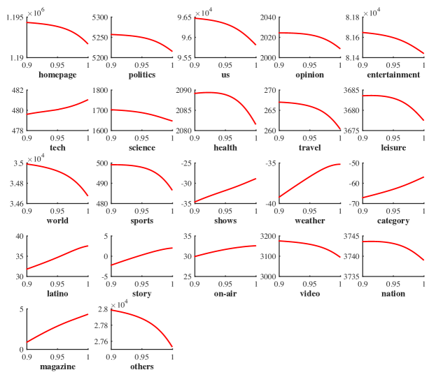
The prior for each baseline discount factor is a smoothness encouraging $Be(19,1)$ truncated to (0.9,0.999); reanalysis using uniform priors on this range led to little in the way of noticeable differences, as the marginal likelihoods at $t=T$ dominate. Running models in parallel across discrete grids of each discount factors and evaluating MML measures at $t=T$ gives marginal likelihoods that are mapped to posteriors. Figure 3 plots posteriors for the $d_{i}$ in the inflow models. Some nodes exhibit higher volatility in flows than others, consistent with smaller discount factors; these are particularly associated with domains with high flow counts (e.g., inflows to Homepage). Constraining the range to higher values is consistent with the expectations to generally “smooth” trajectories for the $\phi_{\ast t}$ processes, which turns out to be consistent with the majority of flows; allowing smaller values has little or no impact on much of the reported analysis. However, for some node flows with patterns of higher levels of change and variation, lower discount factors would lead to posteriors that suggest more volatile trajectories in a few cases. These are better addressed in a model that uses a higher discount factor as standard, but then with interventions to allow increased uncertainty and adaptation in response to discrepant observations (whether single or in batches); our developments in Section 5 are heavily motivated by this. The model is, of course, open to specification of whatever priors a user may regard as relevant or wish to explore.

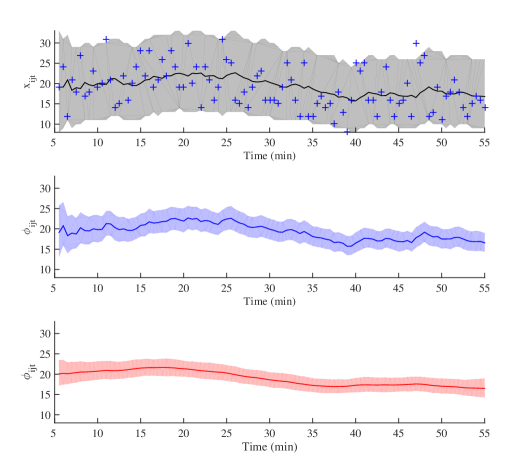
Summary inferences on selected model components are reported from models with discount factors set at posterior modes. Figure 5 gives one example of learning about inflow the Leisure domain. This exemplifies sequential learning about the flow rate together with its retrospectively updated trajectory and a visual assessment of one-step ahead forecasting aligned with the data.

Figure 4: BDFM-based inference on inflows to node $j=10$, the Leisure domain. Upper: data $x_{0,10,t}$ (circles) with one-step ahead forecast means and 95% intervals. Center. trajectory of mean and 95% intervals from on-line posteriors $p(\phi_{0,10,t}|x_{0,10,0{:}t})$. Lower: revised trajectory under full retrospective posterior $p(\phi_{0,10,t}|x_{0,10,0{:}T}).$

Figure 5: BDFM-based inference on transitions from $i=1$ (Homepage) to $j=2$ (Politics). Upper: data $x_{12t}$ (plus signs) with one-step ahead forecast means and 95% intervals. Center. trajectory of mean and 95% intervals from on-line posteriors $p(\phi_{1,2,t}|x_{1,2,0{:}t})$. Lower: revised trajectory under $p(\phi_{1,2,t}|x_{1,2,0{:}T}).$

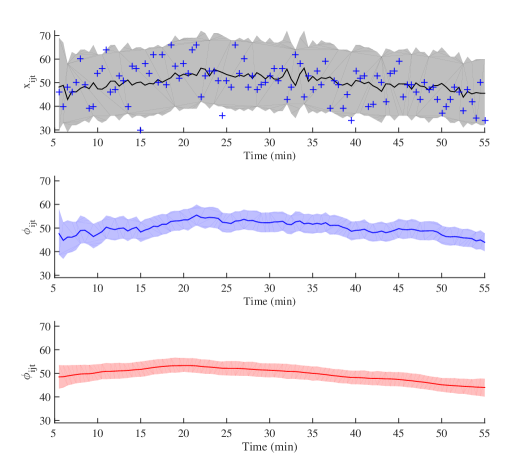
A similar display in Figure 5 is an example of flow between two network nodes: from Homepage to Politics. As with Figure 5, we note the concordance of incoming data with the one-step predictive intervals as they are successively revised in the forward analysis, and the enhanced smoothing of trajectories in the retrospective analysis.

Figure 6: Retrospective posterior means and $95\%$ pointwise intervals of the trajectories of transition probability $\theta_{1,0,t}$ (Homepage $\rightarrow$ External) from analysis on each of the six mornings.

Figure 7: Retrospective posterior means and $95\%$ pointwise intervals of the trajectories of transition probabilities $\theta_{1,5,t}$ (Homepage $\rightarrow$ Entertainment) for each of the six mornings.

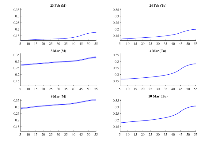
On transition probabilities, it is natural to look at examples involving the Homepage, the most popular single domain on Fox News. For example, Figure 7 shows that the probability of people leaving the Fox News website from Homepage increases in this 50 minute window for each of the six mornings. Note that there are significant day effects; e.g., visitors were more likely to leave Fox News on the morning of March 9th compared to the other mornings. More detailed insights based on the gravity model analysis are noted in Section 4.3. Similar figures (not shown) highlight patterns and day-to-day differences for other transitions. For example, most Homepage visitors stay on Homepage for a while and have a high probability of exiting the Fox News site entirely from that page. Across all six days, the probability of staying on the Homepage each time interval generally decreases over the course of the 50 minute morning period.

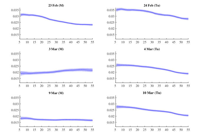
As an illustration of a more detailed analysis of a very specific flow, consider Figure 7. Among the visitors who leave the Homepage for other Fox News domains, Entertainment is generally the most popular destination. Across all mornings, we see major differences in trajectories of transition probabilities; in particular February 23rd and 24th have higher rates than the other days. It is noteworthy that the Academy Awards ceremony was held on the night of February 22nd, which may have driven this uptick. Additional summaries of inference on trajectories of selected $\phi_{ijt}$ and $\theta_{ijt}$ processes appear in the mapping to dynamic gravity models; see the upper row of frames in Figures 10 and 11, for examples.

4 Emulation-Based Mapping to Dynamic Gravity Models

4.1   Dynamic Gravity Models

A more intricate, multivariate dynamic model involves node-specific main effects and node-node interaction terms, representing dependencies in patterns of flows linked to inflow/outflow and node-node relationships. For each within-network node $i=1{:}I$ and all $j=0{:}I,$ the model is

$$\phi_{ijt}=\mu_{t}\ \alpha_{it}\ \beta_{jt}\ \gamma_{ijt}$$ (3)

with: (i) a baseline process $\mu_{t}$; (ii) a node $i$ main effect process $\alpha_{it},$ adjusting the baseline intensity of flows– the origin or outflow parameter process for node $i$; (iii) a node $j$ main effect process $\beta_{jt},$ representing the additional “attractiveness” of node $j$ – the destination or inflow parameter process for node $j$; and (iv) an interaction term $\gamma_{ijt}$, representing the directional “affinity” of node $i$ for $j$ over time relative to the combined contributions of baseline and main effects.

Models of this and more elaborate forms have seen some use in transportation studies (e.g. West 1994; Sen and Smith 1995) where the interaction term is typically structured as a function of physical distance between nodes; there the “gravity model” terminology relates to the role of small distances in defining large interactions and hence “attraction” of traffic from node $i$ to node $j.$ We refer to the $\gamma_{ijt}$ interactions as “affinities”. In dissecting the network flow activity, we are most interested in questions about which affinities are greater than one ($j$ attracts flow from $i$ over and above the main effects), or less than one ($j$ is relatively unattractive to $i$), or not significantly different to one (neutral). Critically, affinities are time-varying, and any identified patterns of variation over time may be related to interpretable events or network changes.

In a first fully Bayesian approach to gravity models using MCMC methods, West (1994) developed such models in the static case; i.e., with no dynamics in the model parameters, and applied the model to a large transportation flow network. Congdon (2000) explored a similar approach in studies of patient flows to hospitals. Analysis via MCMC is computationally very demanding, and the burden increases quadratically in $I$, and inherently non-sequentially. More recently, Jandarov et al. (2014) studied such models for spread of infectious diseases, and used Gaussian process approximations for approximate inference rather than full MCMC or other computational methods.

We share the spirit of this latter work, in using the simply and efficiently implemented BDFM as a path to fitting the gravity model—now extended to time-varying effect parameter processes. However, we do not constrain the affinity parameters $\gamma_{ijt}$ as a function of covariates of any kind, simply treating the DGM as a dynamic, random effects model. This leads to a direct parameter mapping between the BDFM to the DGM; as a result, the trivially generated simulations from the full posterior of the BDFM are mapped directly to full posterior samples from the DGM, providing immediate access to inference on main effect and affinity processes over time.

4.2   Model Mapping for Bayesian Emulation of DGMs by BDFMs

Given a set of flow rates $\phi_{ijt}$ for all $i=1{:}I,j=0{:}I,$ at each time $t=1{:}T,$ the mapping to DGM parameters in eqn. (3) requires aliasing constraints to match dimensions. We adopt the common zero-sum constraint on logged values. Define $h_{t}=\log(\mu_{t})$, $a_{it}=\log(\alpha_{it})$, $b_{jt}=\log(\beta_{jt})$ and $g_{ijt}=\log(\gamma_{ijt}).$ Using the $+$ notation to denote summation over the range of identified indices, constrain via $a_{+t}=b_{+t}=0$, $g_{+jt}=g_{i+t}=0$ for all $i,j,t.$ We then have a bijective map between BDFM and DGM parameters; given the $\phi_{ijt}$ we can directly compute implied, identified DGM parameters. The DGM is saturated– there are exactly as many parameters in the DGM as there are observations in the data set. However, the emulating BDFM enforces smoothness over time in parameter process trajectories, and this acts to substantially reduce the effective model dimension– one key attribute of the emulation approach. Note that this overall strategy inherently adopts the view that temporal structure for DGM parameter processes are those induced by the mapping from BDFMs. In current form, the evolution of latent rate processes in the latter are random walks with levels of variation defined by rate-specific discount factor sequences, so the evolutions for the induced DGM parameters will be more elaborate but still basically of random walk form.

Define $f_{ijt}=\log(\phi_{ijt})$ for each $i=1{:}I,j=0{:}I,$ at each time $t=1{:}T.$ Then at each time $t,$ compute the following in the order given:

• the baseline level $\mu_{t}=\exp(h_{t})$ where $h_{t}=f_{++t}/I(I+1)$;

• for each $i=1{:}I,$ the origin node main effect $\alpha_{it}=\exp(a_{it})$ where $a_{it}=f_{i+t}/(I+1)-h_{t}$;

• for each $j=0{:}I,$ the destination node main effect $\beta_{jt}=\exp(b_{jt})$ where $b_{jt}=f_{+jt}/I-h_{t}$;

• for each $i=1{:}I$ and $j=0{:}I,$ the affinity $\gamma_{ijt}=\exp(g_{ijt})$ where $g_{it}=f_{ijt}-h_{t}-a_{it}-b_{jt}.$

In our data analysis below, we apply this to all simulated $\phi_{ijt}$ from the full posterior analysis under the BDFM to map to posteriors for the DGM parameter processes.

A technical problem with this mapping arises in cases of sparse flows, i.e., when multiple $x_{ijt}$ counts are zero or very small for multiple node pairs. In such cases the posterior for $\phi_{ijt}$ favors very small values and the log transforms are large and negative, which unduly impacts the resulting overall mean and/or origin or destination means. While one can imagine model extensions to address this, at a practical level it suffices to adjust the mapping as is typically done in related problems of log-linear models of contingency tables with structural zeros (Bishop et al. 1975, chap. 5). This is implemented by simply restricting the summations in identifiability constraints to node pairs for which $x_{ijt}>d$, for some small $d,$ and adjusting divisors to count the numbers of terms in each summation. For our study, we use $d=3$. With this adjustment, very small $\phi_{ijt}$ appropriately lead to very small affinities $\gamma_{ijt}$, i.e., small rates underlying very sparse flows.

4.3   Aspects of DGM Analysis of Fox News Data

4.3.1   February 23rd 2015, 09:00–10:00am.

We first apply the gravity model decomposition to the morning data on February 23rd. Following BDFM analysis as in Section 3.4, posterior simulations (5,000 Monte Carlo samples) of flow rates are mapped to posterior samples from the corresponding dynamic gravity model.

Figure 8: Smoothed trajectories of selected node-specific outflows $\alpha_{i,1{:}T}$. The + symbols indicate empirical values computed from the raw data (with cases of 0 occupancy leading to missing values).

Figure 9: Smoothed trajectories of selected node-specific inflows $\beta_{j,1{:}T}$.

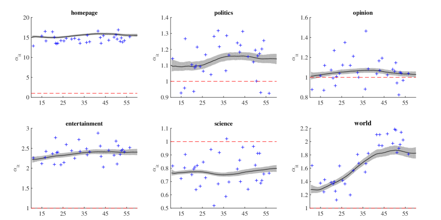
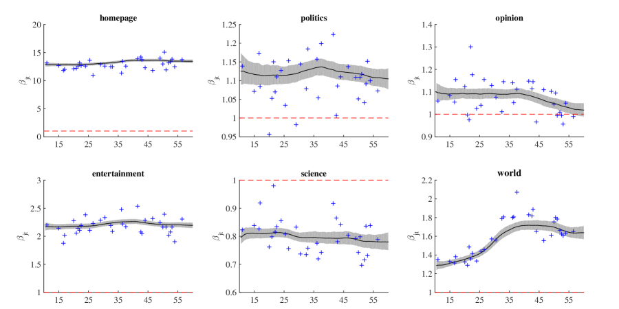
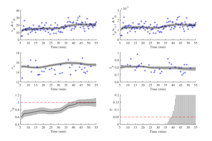
Inference on outflow (origin) parameters $\alpha_{it}$ and inflow (destination) parameters $\beta_{jt}$ for six chosen nodes are shown in Figures 9 and 9. The posteriors for origin effects show that large-scale domains, such Homepage, have higher values of $\alpha_{it}$, while domains with low or zero flows, such as Science, naturally have lower values. Across all domains, subsets show similar patterns but there are also major differences apparent. In particular, the posterior analysis shows that several domains, such as Homepage and Entertainment, are substantially higher than the average as both origin and destination nodes. Several nodes, such as Opinion, have above (or below) average destination effects but origin effects about the norm. These distinctions between the two effects show the roles of $\alpha_{it}$ and $\beta_{jt}$ as representing common factors across the origin and destination of the flows node-by-node. They are also naturally related over time in most domains; this captures the effect of the overall scale, or popularity, of some domains such as Homepage and Entertainment here, while also showing up in clearly similar patterns over time in less active domains, such as World. Further, while some trajectories are relatively stable over time, others show marked changes in the node-specific effects over the morning period. Opinion, for example, has a roughly constant and above-average inflow effect for much of the morning, but it decays toward the end of the morning period; World starts off at a level slightly above the norm in both inflow and outflow effects, which both then increase substantially as the morning progresses; Science, in contrast, has roughly constant effects across the full time period.

For the affinity effects $\gamma_{ijt}$, we have $(I+1)^{2}-1$ parameters (one for each pair of nodes except the unobserved External $\rightarrow$ External flow) at each time $t$. The number of effects becomes massive for large $I$. Even in this example for illustration, $I=22$, the number of $\gamma_{ijt}$ for fixed $t$ is 528, so it is impossible to examine all the results in this paper. For this reason, we pick up a few affinity effects that may interest readers in terms of interpretation. For affinity $\gamma_{ijt}$ with retrospective posterior c.d.f $\Phi_{ijt}(\gamma)$, we introduce the Bayesian credible value $p_{ijt}=\mathrm{min}\{\Phi_{ijt}(1),1-\Phi_{ijt}(1)\}$ as a simple numerical measure of deviation from the “neutral” value of 1. This highlights the practical relevance of the affinity effect and its changes over time.

Traffic from Homepage to other domains are central to understanding normal patterns of variation as Homepage is usually the landing page for visitors. Where users tend to go next, and how the flow patterns begin to evolve from Homepage generally, is one key interest from the advertisement and marketing viewpoints. Figure 10 displays some relevant summaries for flows from Homepage to Science. First, overall counts and also relative frequencies of transitions tend to increase over this morning period. The BDFM appropriately tracks these slowly evolving trends (while not, of course, predicting them). Second, origin/outflow and destination/inflow parameter processes are relatively constant over time, although the former exhibits a slight increase in the later morning period. Of more interest– and highlighting the flexibility and incisiveness of the BDFM$\rightarrow$DGM emulation map– the affinity process is clearly time-varying. Initially at reduced levels– Fox News visitors tend to be much less likely to go to Science from Homepage during the first half or more of the morning period– this trends upwards to be basically negligible in impact after about 35-40minutes. Note that, while the overall outflow and inflow processes are roughly constant over time for this par of nodes, the raw data indicate continued growth in traffic towards the end of the time period, and thus the model responds by inferring the upward drift in the interaction/affinity process.

The pattern over time of the affinity effect also relates to “dynamic sparsity.” While we do not have models that are explicitly exploring sparsity in main or interaction effects, the emulation approach has enabled the identification of an interaction/affinity process that is relevant for some period of time but then, practically, irrelevant for others. In contrast to our easy and scalable methodology, other more formal Bayesian approaches to dynamic sparsity modeling (e.g. Nakajima and West 2013a, b, 2015; Zhou et al. 2014) are difficult or impossible to reliably implement in a sequential context, being reliant on intense MCMC methods for batch data processing. We do note, however, that we are not formally testing consistency of posteriors for affinities against the value of 1, but simply exploring the trajectories to generate insights. More formal assessment is available, if desired, by considering differences in affinities over time from the full posterior sample.

Figure 10: Posterior summaries for DGM parameters for transitions from node $i$=Homepage $\rightarrow j$=Science. As in Figures 9 and 9, the + symbols indicate empirical values (with cases of 0 occupancy leading to missing values). Upper left: Posterior trajectory for the latent flow level process $\phi_{ijt}$ with raw counts (crosses). Upper right: Posterior trajectory for the transition probability process $\theta_{ijt}$ with raw frequencies (crosses). Center left: Posterior trajectory for the Homepage origin (outflow) effect process $\alpha_{it}.$ Center right: Posterior trajectory for the Science destination (inflow) effect process $\beta_{jt}.$ Lower left: Posterior trajectory for the Homepage:Science affinity/interaction process $\gamma_{ijt}$. Lower right: Corresponding trajectories of Bayesian credible values assessing support for $\gamma_{ijt}$ near 1.

Figure 11: Posterior summaries for DGM parameters for transitions from node $i$=Homepage $\rightarrow j$=Entertainment, with details as in Figure 10.

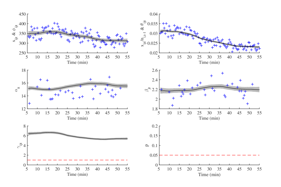
A second example, chosen to represent node pairs with high inflow and outflow levels, concerns transitions from Homepage to Entertainment; see Figure 11. Here again we see that the trivially implemented emulation approach is able to identify a high level of stability over time in the main effects, while indicating subtle changes to reduced levels of affinity in the latter part of the morning period. Considering the downward trending patterns in raw data/relative frequencies of flows from Homepage to Entertainment in the latter period, it would not otherwise be easy to isolate these patterns as idiosyncratic to the node pair. Inferences reflected here on the trajectory of the affinity process clearly show significantly reduced levels later on, with $\gamma_{ijt}$ falling from around 6.5 to around 5.5; relative to the network-wide structure, high affinity is maintained throughout at a practical level, but at a reduced level later on for this node pair.

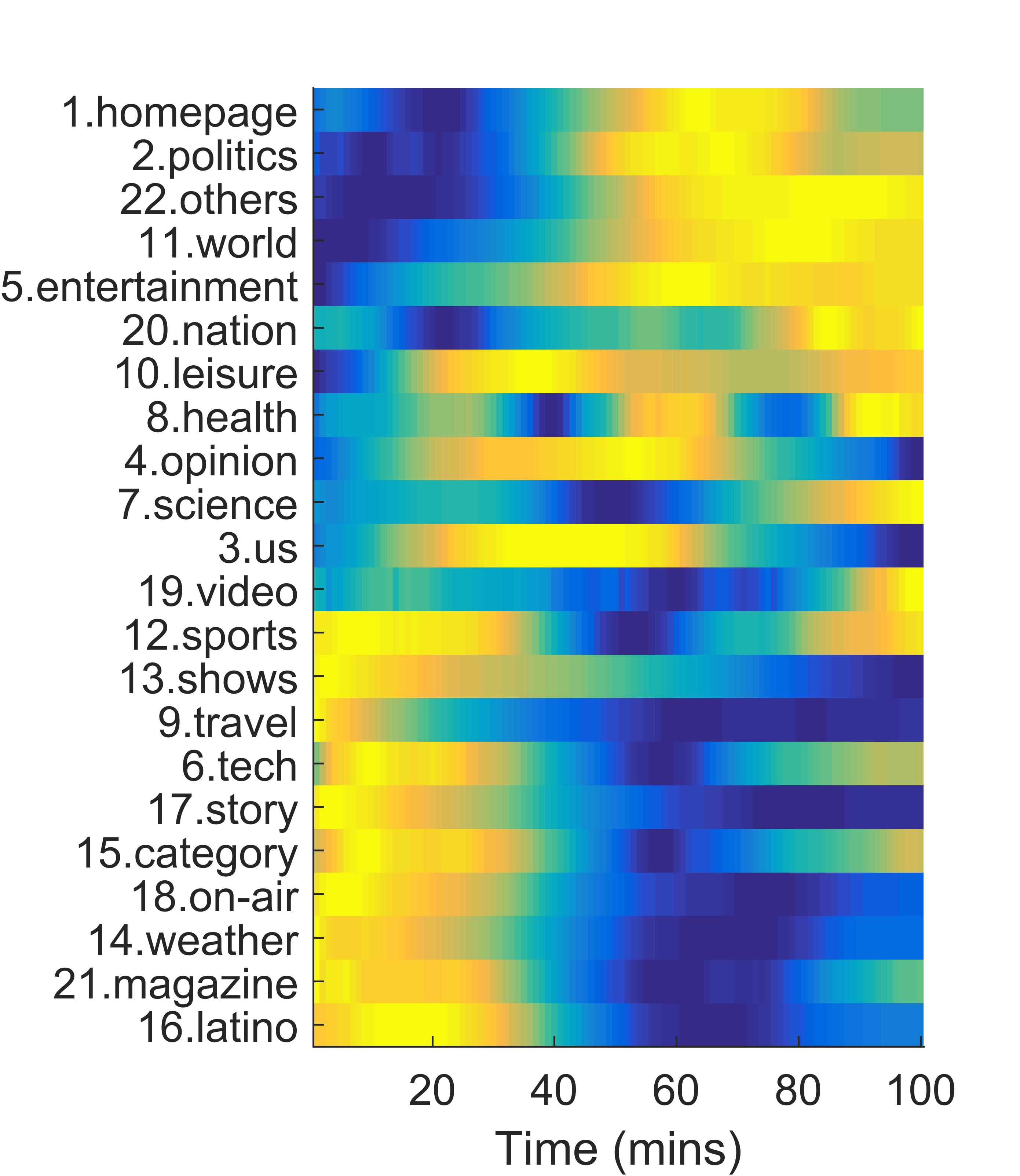
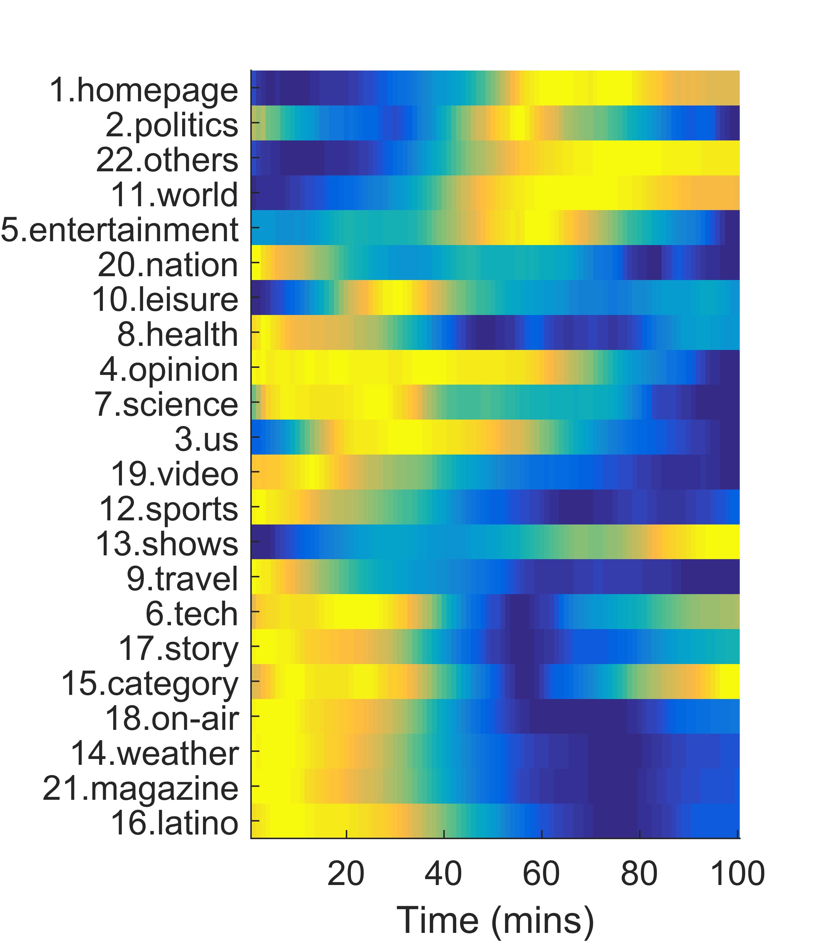
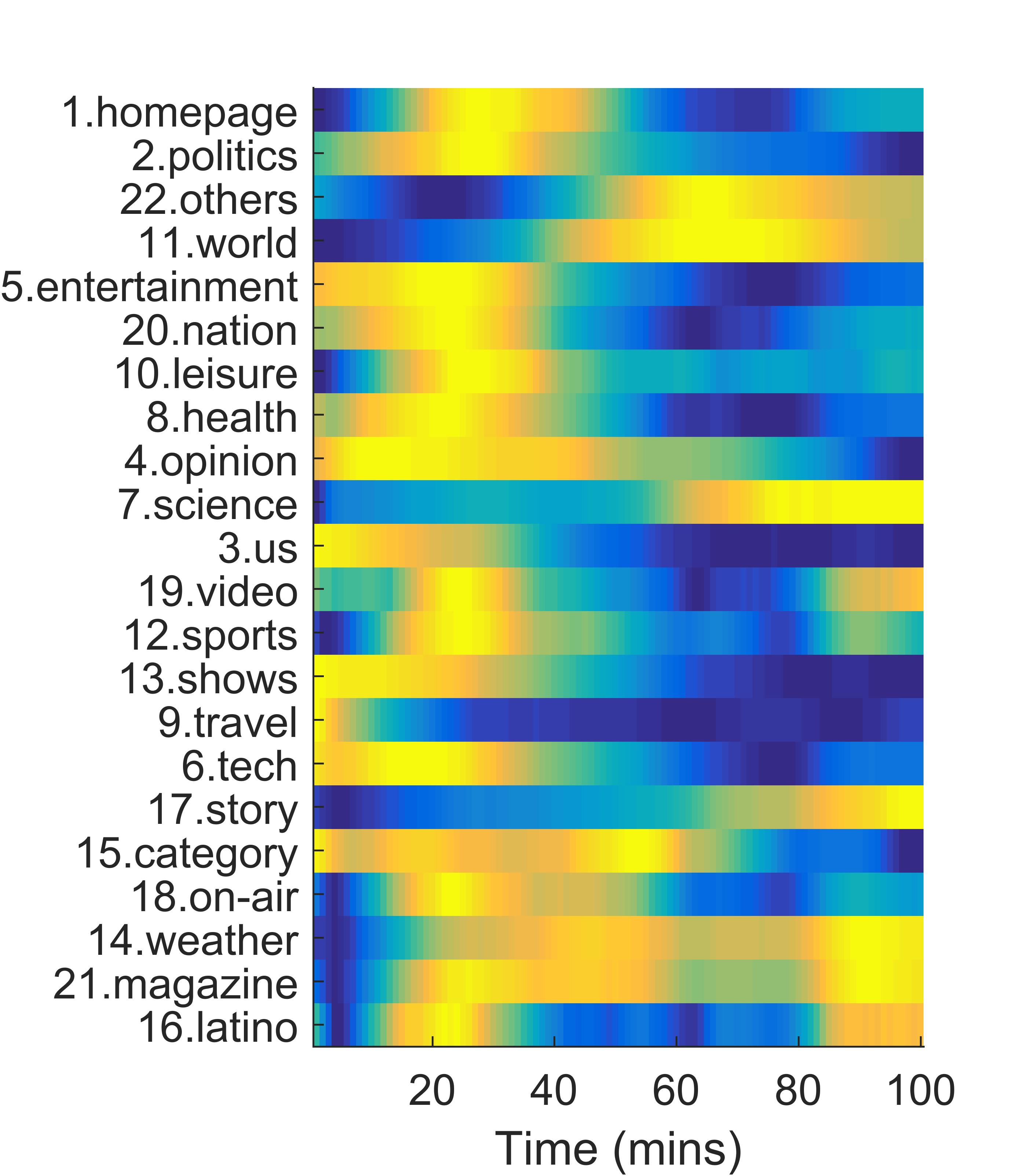
Some heat-maps in Figure 12 show aspects of relationships in some estimated DGM parameters across nodes and across time. These show patterns in the values of the posterior means of $\alpha_{it},\beta_{jt},\gamma_{1jt}$ over time; this includes all main effects and the directional affinities/interactions of all network nodes for flows from domain $1$, the Homepage. Simply for “nice” visual display, the nodes are ordered in terms of correlation over time with the estimated Homepage outflow effect $\alpha_{1t},$ in all three images. The values shown are standardized within each image so that the min/max across time are 0/1. Note common patterns that reflect interdependencies in dynamics across subsets of network nodes. The $\alpha_{it}$ image reflects natural evolution in the morning period of traffic from network nodes, showing the increasing rates of transitions from some of the more popular, core domains (Homepage, Politics, World, Entertainment and others) in later morning. The $\beta_{jt}$ image shows consonant patterns in a subset of these core domains– in that their attractiveness increases in later morning– but with some clearly different cases. For the Homepage affinity processes $\gamma_{1jt},$ there are quite a few domains that see increased incremental traffic rates in the first half, or so, of the morning period, which then drop off to low levels later on.

Outflow effects $\alpha_{it}$	Inflow effects $\beta_{jt}$
Homepage affinities $\gamma_{1jt}$

Figure 12: Heat-map images of standardized posterior means of DGM parameters for all nodes across time in the February 23rd am period. Means are max-min standardized separately for each of the $\alpha_{it}$, $\beta_{jt}$ and $\gamma_{1jt}$ (1=Homepage). Shading runs from 0 (dark grey/dark blue in on-line version) to 1 (white/yellow in on-line version) on these standardized scales. The nodes are ordered based on correlation over time of the main outflow effects $\alpha_{it}$ with that of Homepage; this is an arbitrary ordering chosen simply for visual presentation.

4.3.2   Comparison Across Days.

The study covers morning (09:00–10:00am) and afternoon (01:00–02:00pm) periods on each of 6 days, as already discussed and explored in Section 3.4. Moving to the DGM, we now explore additional features concerning time-of-day effects as well as day-to-day variation. This is based on running the coupled BDFM-DGM analysis separately on each time period/day.

Figure 13 shows the DGM trajectories for the retrospective baseline parameter process $\mu_{1{:}T}$ for each of the 12 fifty-minute intervals. Trajectories are similar across days but for notable differences on February 24th and March 3rd. On February 24th, the afternoon flow is significantly lower than the morning flow, while the morning flow that day is much larger than across other days. One plausible reason is increased morning traffic in response to discussions following the Academy Awards ceremony, with a resulting lull in the afternoon traffic. The reverse happens on March 3 where, although the morning traffic seems typical, the afternoon traffic is unusually high. This was the day on which Fox News posted an article concerning Hillary Clinton’s use of her personal email account for all correspondence during her tenure as Secretary of State. It is plausible that this led to larger than usual afternoon traffic flows as the controversy unfolded.

Figure 13: DGM-based inference on trajectories of baseline flow levels $\mu_{t}$ across days with 95% intervals. Dark/full lines (red in the on-line paper) are for morning periods, lighter/dashed lines are for afternoons.

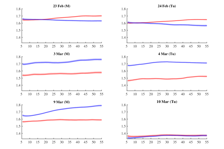
An advantage of the DGM representation is that it allows investigation of such speculative explanations. For example, examination of destination effects (not shown) $\beta_{5,1{:}T}$ confirm that the Entertainment node was unusually popular on February 24th am, and that the Politics and Opinion nodes were unusually popular on March 3 pm, compared to similar flows on other days.

5 Sequential Monitoring of BDFMs and Emulated DGMs

5.1   General Comments

In routine use of dynamic models in sequential monitoring of flows, one key interest is that of being sensitive to data patterns that seem outside the norm, i.e., anomalous, and may reflect events and changes requiring investigation and intervention. We address this here with methodology based on the concepts and theory underlying Bayesian model monitoring in conditionally normal DLMs. While this theory of sequential Bayesian model assessment is well-established, it does not seem to have been adapted to apply to dynamic models of counts; our contributions in this paper include this extension and required customization of the approach.

5.2   Bayesian Model Monitoring and Automated Intervention

Revert to the generic context of a Poisson-gamma model, as in Section3.1 and Appendix A, with time $t$ count observation $x_{t}$ and underlying state $\phi_{t}$. The general strategy here applies to all cases: inflows to any node $j$ when $x_{t}=x_{0jt},$ as well as transitions from a node $i$ to $j$ when $x_{t}=x_{ijt}.$

The sequential Bayesian testing approach in DLMs (West and Harrison 1997, Chapter 11) is extended here to apply to the Poisson-gamma dynamic model. Regard the model as the “standard model” at time $t,$ relabeling the one-step predictive density at each time $t$ as $p_{0}(x_{t}|\delta_{t},\delta_{1{:}t-1},x_{0{:}t-1});$ the suffix 0 indicates the standard model, and we now explicitly recognize the dependence on the discount factors defining levels of stochastic change in the underlying state process $\phi_{t}$. The two components of monitoring and adaptation are as follows.

A. Alternative model predictions: A purely synthetic alternative model at time $t$ that requires only the specification of the alternative predictive p.d.f. $p_{1}(x_{t}|\delta_{t}^{\prime},\delta_{1{:}t-1},x_{0{:}t-1})$, differing from the standard only in the current discount factor $\delta_{t}^{\prime}<\delta_{t}.$ This implies that $p_{1}(\cdot)$ is more diffuse that $p_{0}(\cdot)$ but similarly located. In our Poisson-gamma case, the implied generalized negative binomial p.d.f.s $p_{0}(\cdot)$ and $p_{1}(\cdot)$ have precisely the same mean but the latter has a larger variance and gives more support to both smaller and larger values of $x_{t}$.

B. Bayes factor comparisons: Evaluation of Bayes factors comparing the standard model predictive p.d.f.s with the alternative define the monitoring tests. These marginal likelihood ratios are computed based on both the time $t$ observation and recent consecutive observations to assess and compare consistency of this local data with predictions from the standard model relative to the more diffuse synthetic alternative. Support for the standard model is regarded as a “business as usual” signal. A signal of support for the alternative addresses the potential for: (i) the single observation to be discrepant, a possible outlier; (ii) a relatively abrupt change in the $\phi_{t}$ process at time $t$, beyond that predicted by the model with current discount rate $\delta_{t};$ and (iii) change in the $\phi_{t}$ process at higher levels than the norm, but that are not so abrupt and may have been developing at subtler levels over a few recent time points.

Define the following:

• The time $t$ Bayes factor $H_{t}=p_{0}(x_{t}|\delta_{t},\delta_{1{:}t-1},x_{0{:}t-1})/p_{1}(x_{t}|\delta_{t}^{\prime},\delta_{1{:}t-1},x_{0{:}t-1}),$ assessing the current observation alone.

• The lag-$h$ local Bayes factor $H_{t}(h)=\prod_{r=t-h+1{:}t}p_{0}(x_{r}|\delta_{r},\delta_{1{:}r-1},x_{0{:}r-1})/p_{1}(x_{r}|\delta_{r}^{\prime},\delta_{1{:}r-1}^{\prime},x_{0{:}t-1}).$ based on the most recent $h\in\{1{:}t\}$ observations, including $x_{t}.$

• The local cumulative Bayes factor $L_{t}=\min_{h\in\{1{:}t\}}H_{t}(h)$ and corresponding run-length $l_{t}$ such that $L_{t}=H_{t}(l_{t}).$

Bayesian testing theory (West 1986 and chapter 11 of West and Harrison 1997) shows that the local test measures $L_{t},l_{t}$ are trivially updated as time evolves. At time $t$, the updated pair is

$$[L_{t},\,l_{t}]=\begin{cases}[H_{t},\,1],&\textrm{if }L_{t-1}\geq 1,\\ [H_{t}L_{t-1},\,1+l_{t-1}],&\textrm{if }L_{t-1}<1.\\ \end{cases}$$

Past consistency with the standard model $(L_{t-1}\geq 1)$ means that the entire focus at time $t$ is on the single observation $x_{t}.$ If, however, recent evidence weighs against the standard model $(L_{t-1}<1)$, then that evidence continues to accumulate based on the new observation. The pair $[L_{t},l_{t}]$ define a tracking signal that can be used to formally intervene by rejecting potential outliers and adopting the smaller discount factor $\delta_{t}^{\prime}$ at such times as well as when $L_{t}$ and/or $l_{t}$ suggest cumulating changes in the $\phi_{t}$ process beyond the norm. This operates as follows.

Specify a Bayes factor threshold $\tau$ (e.g. $\tau=0.1$) and run-length threshold $r$ (e.g. $r=4).$ When standing at time $t$, compute single-period Bayes factor $H_{t}$. Then:

• If $H_{t}\leq\tau$, reject $x_{t}$ as potentially outlying.
  $\diamond$ Intervene to apply reduced discount factor $\delta_{t}^{\prime}$ at time $t\to t+1$ in case of changes.

• If $H_{t}>\tau$, then proceed to update $[L_{t},l_{t}]$ to continue monitoring in case of potential changes.

  • If $L_{t}\leq\tau$ or $l_{t}\geq r,$
    $\diamond$ Apply reduced discount factor $\delta_{t}^{\prime}$ to allow for adaptation to potential changes;
    $\diamond$ Update using time $t$ data as usual but with this increased prior uncertainty;
    $\diamond$ Reset monitor to $L_{t}=1$ and $l_{t}=1.$

  • If $L_{t}>\tau$ and $l_{t}<r,$
    $\diamond$ Proceed as usual with prior-posterior and monitor updates.

• Forecast ahead as desired, then proceed to time $t+1.$

This process is displayed in schematic form in Figure 16 of Appendix B, this modified from West and Harrison 1997, Chapter 11, which also discusses choices of thresholds $(\tau,r)$. We follow the recommendations there for these choices. As discussed in Sections 3.2 and 3.3, the discount factors in the standard models are based on $\delta_{t}=d+(1-d)\exp(-kr_{t-1})$ where, in the generic notation here, $r_{t-1}$ is the shape parameter of the time $t-1$ posterior gamma distribution for $\phi_{t-1}$ and $d$ a baseline discount rate. We therefore select the alternative discount factor $\delta_{t}^{\prime}$ for the intervention analysis as $\delta_{t}^{\prime}=d^{\prime}+(1-d^{\prime})\exp(-kr_{t-1})$ where for some smaller baseline $d^{\prime}<d;$ the studies of Fox News network data now mentioned are based on $d=0.1$ whereas the standard models are based on values of $d$ running between 0.9 and 0.99 across the sets of inflow and transition flow models.

5.3   Fox News Network Example

One example from the Fox News study is summarized in Figure 14. While a rather extreme case in terms of one series of time points where the departure from the steady random-walk evolution of the BFDM is very apparent, this example nicely highlights the efficacy of the on-line monitoring and automated intervention strategy. The example is transition flows from Homepage to World over the February 23rd am period.

Figure 14: Summaries from analysis of transitions from node $i$=Homepage $\rightarrow j$=World with Bayesian model monitoring and discount-based intervention. Data is from the February 23rd am period. Upper: Symbol + indicates observations judged consistent with the standard model; x indicates cases identified as potential outliers by low $H_{t}$; * indicates those flagged as potential change points via low $L_{t}$; o indicates cases with $l_{t}>1$. The vertical arrows indicate times of automatic intervention. The full line and shaded region represent one-step forecast means and 95% intervals. Center: Tracks of $\log(H_{t})$ (above center) and $\log(L_{t})$ (below center) over time. Lower: Data (+) with one-step forecast means and 95% intervals from the standard BDFM analysis in light gray (red in on-line version) compared to the analysis with monitoring and intervention in black/dark gray (gray in on-line version).

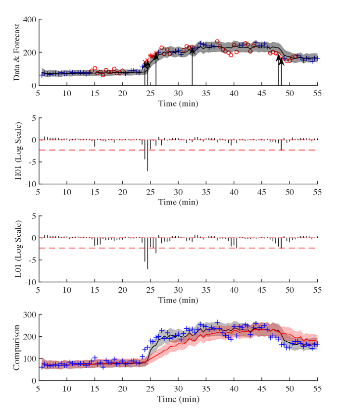
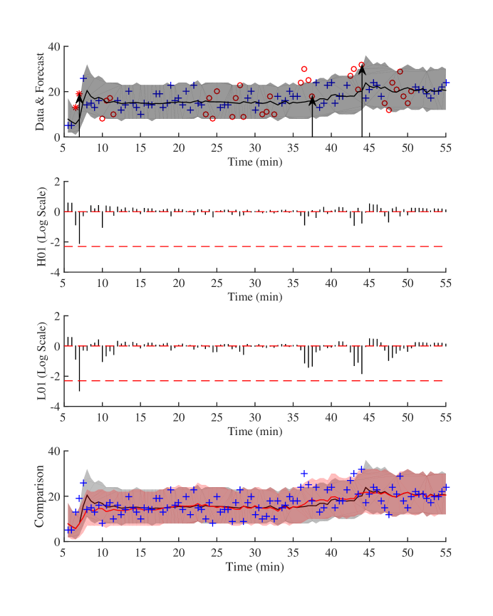
There are several periods in which $l_{t}>1$ but the evidence against the normal model is not so strong as to signal an exception and call for intervention. The period around 23–25minutes saw a substantial upswing in flows that triggered interventions to adapt three times. Interventions at about 32.5 and 48minutes were triggered by a cumulated run-length $l_{t}$ suggesting gradual drift from the standard model. We also note that this picture is very similar when shown in terms of the flow frequencies $x_{ijt}/n_{i,t-1}$ and conditional transition probabilities $\theta_{ijt}$ rather than raw counts $x_{ijt}$ and rates $\phi_{ijt}.$ This is an example where there were (at least) two periods of change in transition characteristics beyond those defined by the BDFM, but that monitoring and intervention is able to adapt to on-line. In a real-life, sequential context, much more can and should be done, of course, at times of intervention. The analysis summary here simply serves to show the potential, recognizing that this is applied in parallel across all inflow and node-node transition models in a wholly automated manner. A second example in Figure 15 shows a somewhat more typical stable trajectory, with only two interventions that appropriately adapt to the modest and subtle level changes in the latter part of the time period.

Figure 15: Summaries from analysis of transitions from node $i$=Homepage $\rightarrow j$=Science under monitoring and intervention, with details as in Figure 14.

6 Closing Comments

The BDFM framework is adaptive to time-varying rates of flows within dynamic networks and able to coherently quantify non-stationary changes in within- and into-/out of- network flow rate processes. This extends and customizes non-stationary process models for count data for transition flows in a network. Novelties include use of relevant occupancy factors to appropriately scale Poisson rates in sets of decoupled models, and the introduction of discount factor scheduling to appropriately address problems with, in particular, low flow rates. Sequential analysis of the resulting Bayesian dynamic flow model is fast and efficient. The decoupled analyses yield full posterior distributions for rate parameter process parameters across nodes and pairs of nodes in a scalable manner. Our analysis of the Fox News network time series data sets shows the utility of the BDFM in generating initial inferences on flow rate processes, in highlighting differences across days and in generating potential practical “leads”. On the latter, for example, it is immediately clear from the BDFM results that most visitors go to just one domain, rather than traversing to multiple domains. This has potential decision implications for computational advertising, and also likely highlights a difference between on-line news consumers and traditional newspaper readers.

The emulation “map” from the BDFM to the DGM represents a strategy of increasing interest in various areas, especially with regard to efficient computation and scalability. We fit a flexible, adaptive model in a set of decoupled analyses, and then directly map posterior samples to the more substantively interesting parameter processes in a model that is otherwise challenging to fit. Applied to the Fox News flow data, we show some (of the many) examples of how this isolates dynamics in node-specific and interaction effects. In some such cases, this indicates “time-varying sparsity” in node-node interaction effects over time, highlighted with our use of Bayesian credible values over time: some interaction effects (affinities) appear significant at some points in time but not in others. A number of the specific node-node inferences mentioned in the application section highlight additional results of substantive interest, some of which are initially unexpected. Others include a sustained positive affinity of Opinion for Homepage, but a similarly sustained but negative affinity of Science for Homepage. Additionally, comparisons across different times of the day and across days identified and quantified patterns related to anomalous flows corresponding to identifiable news events that appear to have driven traffic to specific nodes on the Fox News site.

Computational demands for the full analysis scale as $T(I+1)^{2}n$ where $n$ is the Monte Carlo sample size. Analysis is very fast, based on the core modeling and emulation strategy. A 2016 Matlab implementation running on a standard laptop (2.3GHz cpu, 16Gb memory) took less that 5minutes to run our one period context with $T=110,I=22$ and $n=5{,}000.$ One current interest is in developing this in analysis of a more elaborate, sub-domain network of more than 1,000 nodes, currently under development.

Additional methodological development concerns the use of formal sequential Bayesian model monitoring based on Bayes factor tests, and the accompanying automated intervention analysis to allow models to adapt at time of potential change in underlying flow parameter processes beyond normal levels of variation. Importantly, our use of decoupled/recouple models for within-network transitions allows statistically and computationally efficient development of sequential Bayesian testing based on Bayesian factors related to short-term prediction of each of the individual node-node flows in parallel. At each time point, the decoupled models are monitored, and any signals of significant departure from predictions may be linked across node pairs to explore for dependencies. An unusually significant decrease in inflow to Entertainment at one time, for example, may come via increased transitions from Homepage alone, or represent an Entertainment effect evident in flows from other domains as well. Monitoring and change detection in the decoupled BDFMs can lead to intervention to modify posteriors one or more of the decoupled posteriors for the $\phi_{ijt},$ but the mapping to the DGM parameters will then quantify and highlight the potential relevance for dependencies as well as interaction/affinity effects.

There are now opportunities to use and develop these models as a basis to characterize the stochastic dynamics of website flows, and hence feed into modeling and decision analysis that addresses the needs to respond to changing patterns in computational advertising. An ability to rapidly signal potential anomalies in a small subset of domains in real-time will be of huge interest in this field. More immediately, some of the evident questions arising from the current study concern the overlay of the “unbiased” inferences about changes and structure in network flows with substantive covariate information. In many applications, including computational advertising but also capital and transportation flows, there are useful covariates that could inform the analysis. Our perspective here has been mainly exploratory, aiming to define a formal basis for effectively characterizing non-stationary stochastic dynamics in flow data, and adapting models over time. One next step is to overlay any particular application with covariate information as descriptive/explanatory as we exemplified with some vignettes from the Fox News study. One aspect of this is to consider random effects representing otherwise unexplained extra-Poisson variation that seems relevant in some cases. A more predictive level would involve extensions to incorporate covariates in the BDFMs, so future research in that direction is warranted.

Finally, we note that the general context of time-varying traffic flow analysis arises in multiple other fields. Beyond in origin-destination analysis and related goals in studies of transportation networks  (e.g. Tebaldi and West 1998) and physical traffic (e.g. Tebaldi et al. 2002; Queen and Albers 2009; Anacleto et al. 2013a, b), such data in neural spike train experiments, other varieties of internet traffic, and network studies in areas as diverse as biological anthropology (e.g., grooming interactions in primate troops), human social networks, flows between institutions in finance and economic networks, and others. Our work here represents new methodology of Bayesian dynamic modeling in an application with at least conceptual intersections with some of these areas, and may well be explored in such applications.

Appendix A Appendix: Gamma-Beta Discount Models

This Appendix provides additional details and discussion of the gamma-beta “steady” dynamic model for time-varying Poisson rates, extending the background details underlying the core model summarized in Section 3.1.

Using generic notation, a series of non-negative counts $x_{t}$ over $t=1{:}T$ is modeled via $x_{t}|\phi_{t}\sim Poi(m_{t}\phi_{t})$ conditionally independently over time, where the underlying/latent Poisson rate process $\phi_{t}$ follows a gamma-beta stochastic model and each $m_{t}$ is a scaling constant known at time $t.$ This is effectively a non-stationary, non-Gaussian random walk model, so it has enormous flexibility in adapting to changes over time. The extent of anticipated stochastic change over time is defined by a discount factor parameter $\delta_{t}\in(0,1)$, potentially different at each time $t$. We detail the model concept and structure, and the implied machinery for Bayesian learning and forecasting that includes the forward filtering, backward sampling (FFBS) algorithm for conditionally Poisson time series coupled with the gamma-beta steady process model.

A.1   Forward Filtering (FF)

At time $t=0,$ introduce an hypothetical latent state $\phi_{0}$ and use $x_{0}$ as a synthetic notation for all available initial information. Specify an initial gamma prior, so $\phi_{0}\sim Ga(r_{0},c_{0})$ where $r_{0}>0$, $c_{0}>0$ are known.

For each $t=1{:}T,$ the model and forward/sequential analysis are then as follows.

Posterior at time $t-1$:

Standing at time $t-1$, the posterior for the current Poisson rate given the initial information and all data observed over past times $0{:}t-1$ is gamma,

$$\phi_{t-1}|x_{0{:}t-1}\sim Ga(r_{t-1},c_{t-1})$$ (4)

where the defining parameters are known, evaluated from past information $x_{0{:}t-1}.$

Evolution to time $t$:

The Poisson rate evolves to time $t$ via the gamma-beta evolution

$$\phi_{t}=\phi_{t-1}\eta_{t}/\delta_{t},\qquad\eta_{t}\sim Be(\delta_{t}r_{t-1},(1-\delta_{t})r_{t-1}),$$ (5)

where the random “shock”, or innovation, $\eta_{t}$ is independent of $\phi_{t-1}.$ This is a multiplicative random walk model in that $E(\phi_{t}|\phi_{t-1})=\phi_{t-1},$ hence the use of the “steady model” terminology. A lower value of $\delta_{t}$ leads to a more diffuse beta innovation distribution and the ability to adapt to changing rates over time, while a value closer to one indicates a steady, stable evolution. The random walk nature of the model allows for changes, but does not anticipate specific directional changes. The model results in a fully Bayesian solution to rather simple, flexible smoothing of discrete time series in the context of variation in the underlying latent process.

Note that the beta innovations distribution for $\eta_{t}$ at time $t$ depends in the accumulated information content about the time $t-1$ level through the shape parameter $r_{t-1}.$ The discount factor $\delta_{t}$ acts to decrease the information content between times $t-1$ and $t$ in a natural way. That is, information loss rates are constant over time, rather than parameters of the innovation distribution. The specific choice of beta distribution ensures that the implied time $t$ prior has a conjugate gamma form.

Prior for time $t$:

The time $t-1$ gamma posterior of eqn. (4) couples with the beta innovation to give the time $t-1$ prior for the next state as

$$\phi_{t}|x_{0{:}t-1}\sim Ga(\delta_{t}r_{t-1},\delta_{t}c_{t-1}).$$ (6)

Here we see the discounting effect of the random walk model: the prior for the evolved rate is more diffuse than the time $t-1$ posterior, reflecting increased uncertainty due to evolution.

One-step ahead predictions:

Predicting the data at time $t,$ the one-step ahead forecast distribution is generalized negative binomial with p.d.f.

$$p(x_{t}|x_{0{:}t-1},\delta_{1{:}t})=\frac{\Gamma(\delta_{t}r_{t-1}+x_{t})}{\Gamma(\delta_{t}r_{t-1})\Gamma(x_{t}+1)}\frac{m_{t}^{x_{t}}(\delta_{t}c_{t-1})^{\delta_{t}r_{t-1}}}{(\delta_{t}c_{t-1}+m_{t})^{\delta r_{t-1}+x_{t}}}$$ (7)

on $x_{t}=0,1,\cdots.$

Posterior at time $t$:

Observing $x_{t}$, the resulting posterior is $\phi_{t}|x_{0{:}t}\sim Ga(r_{t},c_{t})$, which has the same form as that at time $t-1$ but with updated parameters $r_{t}=\delta_{t}r_{t-1}+x_{t}$ and $c_{t}=\delta_{t}c_{t-1}+m_{t}$.

A.2   Model Marginal Likelihood (MML)

A key ingredient of formal model assessment is the model marginal likelihood that, in this first-order Markov model, is computed as the product of one-step forecast p.d.f.s evaluated at the realized data. At time $t$, this product is

$$p(x_{1{:}t}|x_{0},\delta_{1{:}t})=\prod_{s=1{:}t}p(x_{s}|x_{0{:}s-1},\delta_{s}).$$

The product is most usefully written in its one-step updated form

$$p(x_{1{:}t}|x_{0},\delta_{1{:}t})=p(x_{t}|x_{0{:}t-1},\delta_{1{:}t})p(x_{1{:}t-1}|x_{0},\delta_{1{:}t-1})$$ (8)

where the contribution at time $t$ derives from the one-step ahead predictive density of eqn. (7) evaluated at the datum $x_{t}.$ These are trivially computed.

One of the most useful roles of the marginal likelihood is in comparing models based on different (sets of) discount factor values. As one key special case, suppose $\delta_{t}=\delta$ is fixed over the time period of interest. Then eqn. (8) gives the value of the marginal likelihood $p(x_{1{:}t}|x_{0},\delta)$ at any chosen value of $\delta.$ In parallel analyses using a discrete set of $\delta$ values, the log of the marginal likelihood is linearly accumulated as data are sequentially processed. At any time $t$ this can be mapped to a posterior $p(\delta|x_{0{:}t})\propto p(\delta|x_{0})p(x_{1{:}t}|x_{0},\delta)$ and then normalized over the grid of values for inference on $\delta$ at any time of interest. This can be used to identify/choose a modal value for inference on the $\phi_{t}$ conditional on a chosen $\delta,$ or for model averaging.

The sequentially computed contributions to the marginal likelihood—the realized p.d.f. ordinates $p(x_{t}|x_{0{:}t-1},\delta)$—can be monitored sequentially over time to provide an on-line tracking of model performance, with potential uses in flagging anomalous data at one node or any subset of nodes, using standard Bayesian model monitoring concepts; see West (1986), West and Harrison (1986, 1989 and Chapter 11 of 1997), and Prado and West (2010, Section 4.3.8).

A.3   Backward Sampling (BS)

Reaching the end time $T$, we look back over time and revise the summary posterior distributions for the full trajectory of the latent gamma process $\phi_{1{:}T}$ based on all the observed data. This uses backward sampling based on theory in West and Harrison (1989b, Section 10.8); see also Prado and West (2010, Section 4.3.7 and problem 4 of Section 4.6).

• Sample the final rate from the time $T$ posterior $\phi_{T}|x_{0{:}T},\delta_{1{:}T}\sim Ga(r_{T},c_{T})$.

• Recurse back over time $t=T-1,T-2,\ldots,1$, at each stage sampling $\phi_{t}$ from the implied $p(\phi_{t}|\phi_{t+1:T},x_{0{:}T},\delta_{1:T})$ via $\phi_{t}=\delta_{t+1}\phi_{t+1}+\epsilon_{t}$ with a “backward innovation” $\epsilon_{t}$ drawn from $\epsilon_{it}\sim Ga((1-\delta_{t+1})r_{t},c_{t})$, independently of $\phi_{t+1}.$

Repeating the backward sampling generates a Monte Carlo sample of the trajectory $\phi_{1{:}T}$ from the full posterior $p(\phi_{1{:}T}|x_{0{:}T},\delta_{1{:}T})$ for summary inferences.

Appendix B Appendix B: Bayesian Model Monitoring and Adaptation

Figure 16: Schematic of monitoring, routine outlier/change assessment and automatic intervention to allow for more adaptability in times of change, as discussed and detailed in Section 5. This relies on a Bayes factor threshold $\tau$ (e.g. $\tau=0.1$) and run-length threshold $r$ (e.g. $r=4).$ This schematic is a modified version of Figure 11.9 in West and Harrison (1997).

References

- Agarwal et al. (2010) D. Agarwal, R. Agrawal, R. Khanna, and N. Kota. Estimating rates of rare events with multiple hierarchies through scalable log-linear models. KDD’10 Proceedings of the 16th ACM SIGKDD, pages 213–222, 2010.
- Ameen and Harrison (1985) J. R. M. Ameen and P. J. Harrison. Normal discount Bayesian models (with discussion). In J. M. Bernardo, M. H. DeGroot, D. V. Lindley, and A. F. M. Smith, editors, Bayesian Statistics 2, pages 271–298. North-Holland, Amsterdam, and Valencia University Press, 1985.
- Anacleto et al. (2013a) O. Anacleto, C. Queen, and C. J. Albers. Forecasting multivariate road traffic flows using Bayesian dynamic graphical models, splines and other traffic variables. Australian and New Zealand Journal of Statistics, 55(2):69–86, 2013. ISSN 1467-842X. doi: 10.1111/anzs.12026.
- Anacleto et al. (2013b) O. Anacleto, C. Queen, and C. J. Albers. Multivariate forecasting of road traffic flows in the presence of heteroscedasticity and measurement errors. Journal of the Royal Statistical Society (Series C: Applied Statistics), 62(2):251–270, 2013. ISSN 1467-9876. doi: 10.1111/j.1467-9876.2012.01059.x.
- Bishop et al. (1975) Y. Bishop, S. E. Fienberg, and P. Holland. Discrete Multivariate Analysis: Theory and Practice. The MIT Press, 1975.
- Brandt et al. (2000) P. T. Brandt, J. T. Williams, B. O. Fordham, and B. Pollins. Dynamic modeling for persistent event-count time series. American Journal of Political Science, 44:823–843, 2000.
- Congdon (2000) P. Congdon. A Bayesian approach to prediction using the gravity model, with an application to patient flow modeling. Geographical Analysis, 32(3):205–224, 2000. ISSN 1538-4632. doi: 10.1111/j.1538-4632.2000.tb00425.x.
- Gruber and West (2016a) L. F. Gruber and M. West. GPU-accelerated Bayesian learning in simultaneous graphical dynamic linear models. Bayesian Analysis, 11:125–149, 2016. doi: 10.1214/15-BA946.
- Gruber and West (2016b) L. F. Gruber and M. West. Bayesian forecasting and scalable multivariate volatility analysis using simultaneous graphical dynamic models. Technical Report, Duke University, 2016. Submitted for publication.
- Harrison and West (1987) P. J. Harrison and M. West. Practical Bayesian forecasting. The Statistician, 36:115–125, 1987.
- Harvey and Fernandes (1989) A. C. Harvey and C. Fernandes. Time series models for count or qualitative observations. Journal of Business and Economic Statistics, 7:409–422, 1989.
- Jandarov et al. (2014) R. Jandarov, M. Haran, O. N. Bjornstad, and B. T. Grenfell. Emulating a gravity model to infer the spatiotemporal dynamics of an infectious disease. Journal of the Royal Statistical Society (Series C: Applied Statistics), 63:423–444, 2014.
- Jansen et al. (2007) B. J. Jansen, A. Spink, and V. Kathuria. How to define searching sessions on web search engines. In O. Nasraoui, M. Spiliopoulou, J. Srivastava, B. Mobasher, and B. Masand, editors, Advances in Web Mining and Web Usage Analysis: 8th International Workshop on Knowledge Discovery on the Web, WebKDD 2006, Lecture Notes in Computer Science, pages 92–109. Springer, 2007.
- Koren et al. (2009) R. Koren, R. Bell, and C. Volinsky. Matrix factorization techniques for recommender systems. Computer, 8:30–37, 2009.
- Nakajima and West (2013a) J. Nakajima and M. West. Bayesian analysis of latent threshold dynamic models. Journal of Business & Economic Statistics, 31:151–164, 2013. doi: 10.1080/07350015.2012.747847.
- Nakajima and West (2013b) J. Nakajima and M. West. Bayesian dynamic factor models: Latent threshold approach. Journal of Financial Econometrics, 11:116–153, 2013. doi: 10.1093/jjfinec/nbs013.
- Nakajima and West (2015) J. Nakajima and M. West. Dynamic network signal processing using latent threshold models. Digital Signal Processing, 47:6–15, 2015. doi: 10.1016/j.dsp.2015.04.008.
- Pang and Lee (2008) B. Pang and L. Lee. Opinion mining and sentiment analysis. Foundations and Trends in Information Retrieval, 2(455):1–135, 2008.
- Prado and West (2010) R. Prado and M. West. Time Series: Modeling, Computation and Inference. Chapman & Hall/CRC Press, 2010.
- Qiu et al. (2005) F. Qiu, Z. Liu, and J. Cho. Analysis of user web traffic with a focus on search activities. In Proceedings of the Eight International Workshop on the Web & Databases (WebDB 2005), pages 103–108, 2005.
- Queen and Albers (2009) Catriona M. Queen and Casper J. Albers. Intervention and causality: Forecasting traffic flows using a dynamic Bayesian network. Journal of the American Statistical Association, 104:669–681, 2009. doi: 10.1198/jasa.2009.0042.
- Quintana and West (1987) J. M. Quintana and M. West. An analysis of international exchange rates using multivariate DLMs. The Statistician, 36:275–281, 1987.
- Sen and Smith (1995) A. Sen and T. Smith. Gravity Models of Spatial Interaction Behavior. Springer, 1995.
- Silverstein et al. (1999) C. Silverstein, H. Marais, M. Henzinger, and M. Moricz. Analysis of a very large web search engine query log. SIGIR Forum, 33:6–12, 1999. doi: 10.1145/331403.331405.
- Smith (1979) J. Q. Smith. A generalization of the bayesian steady forecasting model. Journal of the Royal Statistical Society (Series B: Methodological), 41:375–387, 1979.
- Soriano et al. (2013) J. Soriano, T. Au, and D. Banks. Text mining in computational advertising. Statistical Analysis and Data Mining, 6:273–285, 2013.
- Taddy (2013) M. Taddy. Multinomial inverse regression for text analysis. Journal of the American Statistical Association, 108:755–770, 2013.
- Tebaldi and West (1998) C. Tebaldi and M. West. Bayesian inference on network traffic using link count data (with discussion). Journal of the American Statistical Association, 93:557–576, 1998.
- Tebaldi et al. (2002) C. Tebaldi, M. West, and A. F. Karr. Statistical analyses of freeway traffic flows. Journal of Forecasting, 21:39–68, 2002.
- West (1986) M. West. Bayesian model monitoring. Journal of the Royal Statistical Society (Series B: Methodological), 48:70–78, 1986.
- West (1994) M. West. Statistical inference for gravity models in transportation flow forecasting. Discussion Paper 94-20, Institute of Statistics & Decision Sciences, Duke University (June 1994), and NISS Technical Report #60, US National Institute of Statistical Sciences, 1994.
- West and Harrison (1986) M. West and P. J. Harrison. Monitoring and adaptation in Bayesian forecasting models. Journal of the American Statistical Association, 81:741–750, 1986.
- West and Harrison (1989a) M. West and P. J. Harrison. Subjective intervention in formal models. Journal of Forecasting, 8:33–53, 1989.
- West and Harrison (1989b) M. West and P. J. Harrison. Bayesian Forecasting & Dynamic Models. Springer, 1st edition, 1989.
- West and Harrison (1997) M. West and P. J. Harrison. Bayesian Forecasting and Dynamic Models. Springer, 2nd edition, 1997.
- Zhao et al. (2016) Z. Y. Zhao, M. Xie, and M. West. Dynamic dependence networks: Financial time series forecasting & portfolio decisions (with discussion). Applied Stochastic Models in Business and Industry, 2016. doi: 10.1002/asmb.2161. First published online: March 25, 2016.
- Zhou et al. (2014) X. Zhou, J. Nakajima, and M. West. Bayesian forecasting and portfolio decisions using dynamic dependent sparse factor models. International Journal of Forecasting, 30:963–980, 2014. doi: http://dx.doi.org/10.1016/j.ijforecast.2014.03.017.