Interpreting the cosmic far-infrared background anisotropies using a gas regulator model

Abstract

Cosmic far-infrared background (CFIRB) is a powerful probe of the history of star formation rate (SFR) and the connection between baryons and dark matter across cosmic time. In this work, we explore to which extent the CFIRB anisotropies can be reproduced by a simple physical framework for galaxy evolution, the gas regulator (bathtub) model. This model is based on continuity equations for gas, stars, and metals, taking into account cosmic gas accretion, star formation, and gas ejection. We model the large-scale galaxy bias and small-scale shot noise self-consistently, and we constrain our model using the CFIRB power spectra measured by Planck. Because of the simplicity of the physical model, the goodness of fit is limited. We compare our model predictions with the observed correlation between CFIRB and gravitational lensing, bolometric infrared luminosity functions, and submillimetre source counts. The strong clustering of CFIRB indicates a large galaxy bias, which corresponds to haloes of mass $10^{12.5}\rm M_{\odot}$ at $z=2$, higher than the mass associated with the peak of the star formation efficiency. We also find that the far-infrared luminosities of haloes above $10^{12}\rm M_{\odot}$ are higher than the expectation from the SFR observed in ultraviolet and optical surveys.

1 Introduction

Cosmic far-infrared background (CFIRB) originates from unresolved dusty star-forming galaxies across cosmic time. In these galaxies, the ultraviolet (UV) photons associated with newly formed, massive stars are absorbed by dust and re-emitted in far-infrared (FIR), and the FIR emission serves as an indicator of the star formation rate (SFR). At the FIR wavelengths ($\sim$100 µm to 1 mm, also known as submillimetre), most galaxies are unresolved and can only be observed as background intensity fluctuations. These fluctuations contain information about the cosmic star formation history, as well as the dark matter haloes in which the dusty star-forming galaxies are located. Compared with UV, the star formation history from FIR is much less explored because of the limited angular resolutions of the telescopes; thus, CFIRB provides an important piece of the puzzle of the cosmic star formation history.

Predicted half a century ago (Partridge & Peebles, 1967; Bond et al., 1986), the CFIRB was first discovered by COBE-FIRAS (Puget et al., 1996; Fixsen et al., 1998; Hauser et al., 1998; Gispert et al., 2000; Hauser & Dwek, 2001) and subsequently observed by ISO (Lagache & Puget, 2000; Matsuhara et al., 2000; Elbaz et al., 2002). The anisotropies of CFIRB have been measured by Spitzer (Grossan & Smoot, 2007; Lagache et al., 2007), BLAST (Viero et al., 2009), SPT (Hall et al., 2010), ACT (Hajian et al., 2012), Herschel (Amblard et al., 2011; Berta et al., 2011; Viero et al., 2013a), and Planck (Planck Collaboration XVIII, 2011; Planck Collaboration XXX, 2014). In particular, the angular power spectra of CFIRB provide the luminosity-weighted galaxy bias and thus the information about the mass of the underlying dark matter haloes (e.g., Viero et al., 2009; Amblard et al., 2011; Planck Collaboration XVIII, 2011; De Bernardis & Cooray, 2012; Shang et al., 2012; Xia et al., 2012; Thacker et al., 2013; Viero et al., 2013a; Planck Collaboration XXX, 2014).

To date, most of the interpretations of the CFIRB anisotropies are based on phenomenological models with limited physical interpretation. For example, Addison et al. (2013) modelled the CFIRB and number counts using general parametrizations for the luminosity function, the spectral energy distribution (SED), and the scale-dependent galaxy bias. On the other hand, Shang et al. (2012) implemented a luminosity–mass relation in the halo model to improve the modelling at small scales (also see, e.g., Viero et al., 2013a). In addition, Planck Collaboration XXX (2014) provided updated measurements of the CFIRB power spectra as well as new constraints on linear and halo models; however, the SFR density inferred from their halo model appears higher at high redshift when compared with UV and optical observations.

In this work, we develop a physical model for the connection between dark matter haloes and dusty star-forming galaxies. We constrain this model using the CFIRB power spectra measured by Planck. We then compare our model with various FIR/submillimetre galaxy observations. Our model provides a simple, physically-motivated framework to compare and interpret various FIR observations.

We apply the gas regulator model, which is based on the continuity equations of gas, stars, and metal (also known as the bathtub or reservoir model, see, e.g., Bouché et al., 2010; Krumholz & Dekel, 2012; Dekel et al., 2013; Lilly et al., 2013; Dekel & Mandelker, 2014), to calculate SFR. We then apply the halo model to calculate the power spectra of CFIRB (Scherrer & Bertschinger, 1991; Seljak, 2000; Cooray & Sheth, 2002). We fit the model to the CFIRB anisotropies measured by Planck (Planck Collaboration XXX, 2014). Our model predictions are compared with various IR observations, as well as the cosmic SFR density and cosmic dust mass density constrained by other observations. We find that CFIRB requires high IR luminosity for massive haloes ($L_{\rm IR}\sim 10^{12}\rm L_{\odot}$ for haloes of mass above $10^{13}\rm M_{\odot}$); this result is consistent with earlier findings (e.g., Shang et al., 2012; Addison et al., 2013; Béthermin et al., 2013) but is in excess compared with the SFR constrained by UV and optical. This excess of IR luminosity can be related to heating by old stellar populations.

This paper is organized as follows. Section 2 describes the gas regulator model and provides a quasi-steady-state solution relevant for SFR and dust property. In Section 3, we incorporate the gas regulator model into the halo model to calculate observed quantities. In Section 4, we fit our model to the CFIRB angular power spectra and intensity. Section 5 shows comparisons between our model and other infrared observations. In Section 6, we discuss the implications of our model, including the galaxy–halo connection and the cosmic star formation history; in Section 7, we discuss the limitations of our model and possible improvements. We summarize in Section 8.

Throughout this paper, we use a flat $\Lambda$CDM cosmology based on the Planck 2013 results (Planck Collaboration XVI, 2014); $\Omega_{M}$ = 0.31; $\Omega_{\Lambda}$ = 0.69; $h$ = 0.67. We use the linear matter power spectrum at $z=0$ calculated by CAMB (Lewis et al., 2000) with $\Omega_{b}h^{2}=0.022$; $\Omega_{c}h^{2}=0.12$; $n_{s}=0.96$; $A_{s}=2.215\times 10^{-9}$. When converting SFR to IR luminosity, we use $L_{\rm IR}={\rm SFR}/{K}$, where $K=1.7\times 10^{-10}\ \rm M_{\odot}\ \rm yr^{-1}\ \rm L_{\odot}^{-1}$ based on the Salpeter initial mass function (Kennicutt, 1998).

2 Gas regulator model for galaxy evolution

In the gas regulator model, a galaxy is assumed to be a reservoir of gas, stars, and metal; the mass of each component is determined by a continuity equation with sources (cosmic accretion), sinks (star formation), and outflow. This model assumes that both the SFR and the gas outflow rate are proportional to the gas mass; therefore, the system is self-regulated and will eventually reach a steady state (e.g., Bouché et al., 2010; Dekel et al., 2013; Lilly et al., 2013). Our model is based on the minimal implementation in Dekel & Mandelker (2014, DM14 thereafter) with various modifications. Table 1 summarizes the physical processes in this model, and Table 2 lists the parameters in this model.

2.1 Basic model and quasi-steady-state solution

To describe the source terms, let us denote the cosmic accretion rate of all baryon mass as $\dot{M}_{\rm a}$. In this accreted baryon mass, we assume that the gas mass fraction is $f_{\rm ga}$, and the stellar mass fraction is $(1-f_{\rm ga})$. Star formation converts gas mass to stellar mass. We denote the SFR of the galaxy as $\dot{M}_{\rm sf}$; since stars return a fraction (denoted as $R$) of the gas to the reservoir, the gas consumption rate is given by $(1-R)\dot{M}_{\rm sf}$. In addition, the gas mass can be ejected from the galaxy due to feedback processes, and we assume that the mass-loss rate is proportional to the SFR, $\eta\dot{M}_{\rm sf}$. Here, $\eta$ is the mass-loading factor and will be discussed in detail in Section 2.3. We assume that the outflow of stellar mass is negligible.

The continuity equations of gas mass ($M_{\rm g}$) and stellar mass ($M_{\rm s}$) are given by

$$\dot{M}_{\rm g}=f_{\rm ga}\dot{M}_{\rm a}-(1-R+\eta)\dot{M}_{\rm sf}\ ,$$ (1)

and

$$\dot{M}_{\rm s}=(1-f_{\rm ga})\dot{M}_{\rm a}+(1-R)\dot{M}_{\rm sf}\ .$$ (2)

Since the stellar mass is not directly observable in FIR, we will not further discuss the stellar mass in this paper.

We assume that the cosmic accretion provides negligible metal mass. The metal production rate is given by $y(1-R)\dot{M}_{\rm sf}$, where $y$ is the metal yield. The loss of metal is proportional to the loss of gas. The continuity equation of metal mass ($M_{\rm m}$) is thus given by

$$\dot{M}_{\rm m}=y(1-R)\dot{M}_{\rm sf}-(1-R+\eta)\dot{M}_{\rm sf}\frac{M_{\rm m}}{M_{\rm g}}\ .$$ (3)

For the quasi-steady-state solution, we assume $\dot{M}_{\rm g}=0$ and $\dot{M}_{\rm m}=0$. Equations (1) and (3) become

$$\dot{M}_{\rm sf}=\frac{f_{\rm ga}\dot{M}_{\rm a}}{1-R+\eta}$$ (4)

and

$$M_{\rm m}=M_{\rm g}\frac{y(1-R)}{1-R+\eta}\ .$$ (5)

Under this assumption, the gas metallicity $M_{\rm m}/M_{\rm g}$ is constant with time.

To calculate the gas mass, we assume that $\dot{M}_{\rm sf}=M_{\rm g}/t_{\rm sf}$, where $t_{\rm sf}$ is the star formation time-scale,

$$M_{\rm g}=\frac{f_{\rm ga}\dot{M}_{\rm a}t_{\rm sf}}{1-R+\eta}\ .$$ (6)

Physical process	Gas	Star	Metal in gas
Cosmic accretion	$f_{\rm ga}\dot{M}_{\rm a}$	$(1-f_{\rm ga})\dot{M}_{\rm a}$	(Negligible)
Star formation	$-(1-R)\dot{M}_{\rm sf}$	$(1-R)\dot{M}_{\rm sf}$	$y(1-R)\dot{M}_{\rm sf}-(1-R)\dot{M}_{\rm sf}M_{\rm m}/M_{\rm g}$
Outflow	$-\eta\dot{M}_{\rm sf}$	(Negligible)	$-\eta\dot{M}_{\rm sf}M_{\rm m}/M_{\rm g}$

Table 1: Summary of source, sink, and outflow terms in the gas regulator model.

Parameter	Meaning	Fiducial value	Reference
	Cosmic accretion
$f_{b}$	$\Omega_{b}/\Omega_{M}$	0.18	Planck Collaboration XVI (2014)
$f_{\rm ga}$	(gas mass) / (gas mass + stellar mass) in cosmic accretion, $0<f_{\rm ga}<1$	0.8	Dekel & Mandelker (2014)
$\dot{M}_{\rm a}$	Accretion rate of all baryon mass	–	ibid.
$p$	Penetration factor, $M_{\rm accreted\ baryon}/(f_{b}M_{\rm accreted\ DM})$	0.5	ibid.
	Star formation
$K$	$L_{\rm IR}={\rm SFR}/K$	$1.7\times 10^{-10}$	Kennicutt (1998)
$\dot{M}_{\rm sf}$	SFR	–	Dekel & Mandelker (2014)
$t_{\rm sf}$	Star formation time-scale $t_{\rm sf}=\epsilon^{-1}t_{d}$	–	ibid.
$\epsilon$	SFR efficiency per dynamical time	0.02	ibid.
$t_{d}$	Dynamical time, $t_{d}=\nu_{d}t$, where $t$ is the cosmic time	–	ibid.
$\nu_{d}$	$t_{d}$ in units of the cosmological time	0.0071	ibid.
$R$	Fraction of gas mass returned by star formation	0.46	ibid.
$\eta$	Mass-loading factor, ratio between gas outflow and SFR	–	equation (16)
	Metal and dust
$y$	Metal yield	0.016	Lilly et al. (2013)
$r$	Dust-to-metal mass density ratio	0.4	Hayward et al. (2011)
	Dust SED
$\beta$	Spectral index of dust SED	(2)	ibid.
$\kappa$	Dust opacity, $\kappa=\kappa_{0}(\nu/\nu_{0})^{\beta}$	–	Hayward et al. (2011)
$\kappa_{0}$	Opacity at the pivot frequency	0.050	ibid.
$\nu_{0}$	Pivot frequency for opacity	850$\micron$	ibid.
	Halo mass – IR luminosity relation
$M_{\rm pk}$	Peak halo mass for SFR	$10^{12}\rm M_{\odot}$	Behroozi et al. (2013)
$M_{\rm min}$	Minimum halo mass for hosting a FIR galaxy	$10^{11}\rm M_{\odot}$	Krumholz & Dekel (2012)

Table 2: Parameters in the gas regulator model. Numbers in parentheses indicate the values used in the references; these parameters are set free in our model.

2.2 Implementation

Equation (4) is our prediction for the SFR. We assume that the baryon mass accretion rate $\dot{M}_{\rm a}$ is proportional to the dark matter accretion rate

$$\dot{M}_{\rm a}=f_{b}p\dot{M}_{\rm h}\ ,$$ (7)

where $M_{\rm h}$ is the mass of the dark matter halo; $f_{b}$ is the cosmic baryon mass fraction $\Omega_{b}/\Omega_{M}$, which is assumed to be 0.18 (Planck Collaboration XVI, 2014); $p$ indicates the mass fraction of the gas that can penetrate the halo and reach the galaxy.

For the mass accretion rate of dark matter haloes, we use the fitting formula calibrated using the two Millennium simulations by Fakhouri et al. (2010)

$$\dot{M_{\rm h}}= 46.1{\rm M_{\odot}yr^{-1}}\bigg{(}\frac{M}{10^{12}\rm M_{\odot}}\bigg{)}^{1.1}$$ (8)

$$\times(1+1.11z)\sqrt{\Omega_{M}(1+z)^{3}+\Omega_{\Lambda}}.$$

We include an extra redshift dependence to model the fact that the SFR does not necessarily trace the gas accretion rate,

$$f(z)=(1+z)^{\delta}\ .$$ (9)

We assume that $\dot{M}_{\rm sf}$ is proportional to the IR luminosity,

$$L_{\rm IR}=\frac{\dot{M}_{\rm sf}}{K}\ ,$$ (10)

where $K=1.7\times 10^{-10}\ \rm M_{\odot}\ \rm yr^{-1}\ \rm L_{\odot}^{-1}$ (Kennicutt, 1998, based on the Salpeter initial mass function).

To summarize, the $L_{\rm IR}$–halo mass relation is given by

$$L_{\rm IR}=\frac{f_{\rm ga}f_{b}p}{K(1-R+\eta)}\dot{M_{\rm h}}f(z).$$ (11)

We assume that the dust mass is proportional to the metal mass with a constant dust-to-metal ratio, $r=M_{\rm d}/M_{\rm m}$, and is given by

$$M_{\rm d}=\frac{ry(1-R)}{1-R+\eta}t_{\rm sf}\dot{M}_{\rm sf}=\frac{ry(1-R)}{(1-R+\eta)^{2}}f_{\rm ga}f_{b}p\dot{M_{\rm h}}f(z)t_{\rm sf}\ .$$ (12)

Following DM14, we assume that the star formation time-scale is proportional to the dynamical time, $t_{\rm sf}=\epsilon^{-1}t_{d}$, and $\epsilon=0.02$. The dynamical time is assumed to be proportional to the cosmic time, $t_{d}=\nu t$, and $\nu=0.0071$.

We assume that the spectral luminosity is given by an optically-thin modified blackbody with a single dust temperature $T_{\rm d}$ (e.g., Hayward et al., 2011)

$$L_{\nu}=4{\rm\pi}\kappa_{\nu}M_{\rm d}B_{\nu}(T_{\rm d})\ ,$$ (13)

and that the opacity in IR follows a power-law

$$\kappa_{\nu}=\kappa_{0}\bigg{(}\frac{\nu}{\nu_{0}}\bigg{)}^{\beta}\ .$$ (14)

Integrating $L_{\nu}$ over $\nu$, we obtain $L_{\rm IR}$ as a function of $M_{\rm d}$ and $T_{\rm d}$. Solving for $T_{\rm d}$, we obtain

$$T_{\rm d}=\frac{h}{k}\bigg{[}\frac{L_{\rm IR}c^{2}\nu_{0}^{\beta}}{\Gamma(4+\beta)\zeta(4+\beta)8{\rm\pi}\kappa_{0}hM_{\rm d}}\bigg{]}^{1/(4+\beta)}\ .$$ (15)

Following Hayward et al. (2011), we assume that $\kappa_{0}=0.07\ {\rm m^{2}kg^{-1}}$ at $850\ \micron$ at observed frame, $\nu_{0}=353\ (1+z)\ {\rm GHz}$. The spectral index $\beta$ is a free parameter in our model. Since we are only concerned with the FIR wavelengths in the Rayleigh–Jeans tail, we expect that the single-temperature modified blackbody is a reasonable description for our SED.

2.3 Modelling feedback via mass-loading factor

Equation (4) indicates that the SFR is determined by the mass accretion rate; however, additional feedback processes can affect the SFR. For low-mass haloes, supernova feedback can eject gas efficiently and suppress the SFR (e.g., Benson et al., 2003; Dutton & van den Bosch, 2009). To model this effect, we assume $\eta\propto M_{\rm h}^{-\alpha_{1}}$ for $M_{\rm h}<M_{\rm pk}$, where $M_{\rm pk}$ is the halo mass associated with the peak of the star formation efficiency.

Different values of $\alpha_{1}$ correspond to different physical models for supernova feedback. For example, for energy-driven winds, $\eta\propto V_{\rm vir}^{-2}\propto M_{\rm vir}^{-2/3}$ (e.g., Benson, 2010); for momentum-driven winds, $\eta\propto V_{\rm vir}^{-1}\propto M_{\rm vir}^{-1/3}$ (e.g., Murray et al., 2005; Hopkins et al., 2012); for constant winds, $\eta$ = constant (e.g., Springel & Hernquist, 2003). Steeper scaling relations have also been adopted by some semi-analytical models (e.g., Guo et al., 2011). Observations have been used to estimate the velocities of gas outflow; however, constraining the mass dependence of the mass-loading factor is still challenging (e.g., Weiner et al., 2009; Chen et al., 2010; Martin et al., 2012; Rubin et al., 2014, see Veilleux et al. 2005; Erb 2015 for reviews).

For massive haloes, the SFR is suppressed by feedback from active galactic nuclei (e.g., Croton et al., 2006) or quenched due to environment (e.g., Wetzel et al., 2012). Thus, for massive haloes ($M_{\rm h}>M_{\rm pk}$), we phenomenologically model the mass-loading factor as $\eta\propto M^{\alpha_{2}}$; this parametrization effectively describes the reduced supply of cold gas. In addition, observations have hinted that SFR and the AGN luminosity is related to each other (Lutz et al., 2010), supporting the gas regulator model in the regime of AGN feedback.

To make the transition between high- and low-mass smooth, we adopt the function form (see, e.g., Feldmann, 2015)

$$\eta(M)=f(x,y)=\eta_{0}\bigg{(}1+x+y-(1+x^{-1}+y^{-1})^{-1}\bigg{)}\ ,$$ (16)

where

$$x=\bigg{(}\frac{M_{\rm h}}{M_{\rm pk}}\bigg{)}^{-\alpha_{1}},\quad y=\bigg{(}\frac{M_{\rm h}}{M_{\rm pk}}\bigg{)}^{\alpha_{2}}\ .$$ (17)

We assume $M_{\rm pk}=10^{12}\rm M_{\odot}$ (see e.g., Behroozi et al. 2013) and use three free parameters to describe the mass-loading factor: ($\eta_{0}$, $\alpha_{1}$, $\alpha_{2}$).

3 Halo model for clustering

Given the $L_{\rm IR}$–$M_{\rm h}$ relation and the SED from the gas regulator model, we can apply the halo model to calculate the CFIRB power spectra and various FIR observables. We include the scatter between IR luminosity and halo mass.

3.1 CFIRB Intensity and power spectra

We denote $\nu$ as the frequency in the observed frame. For brevity, we denote $L_{\rm IR}$ as $L$ and $M_{\rm h}$ as $M$ below. The emission coefficient at $\nu$ at redshift $z$ is given by integrating the spectral luminosity of all haloes, described by the halo mass function ($dn/dM$), at this redshift,

$$j_{\nu}(z)=\int dM\frac{dn}{dM}f_{\nu}(M,z)\ ,$$ (18)

where

$$f_{\nu}(M,z)=\frac{1}{4{\rm\pi}}L_{(1+z)\nu}(M,z)\ .$$ (19)

We note that here $L_{(1+z)\nu}$ includes the contribution from both central and satellite galaxies, because in the gas regulator model we calculate the accretion rate of the entire host halo. This is a major difference between our model and the model in Shang et al. (2012).

The spectral intensity is given by integrating the emission coefficient over all redshifts,

$$I_{\nu}=\int dz\frac{d\chi}{dz}aj(z)\ ,$$ (20)

where $a=1/(1+z)$ is the scale factor, and $\chi$ is the comoving distance.

The angular power spectra at large scale are determined by galaxy pairs in two different haloes, i.e., the two halo term, which is given by

$$C^{2h}_{\ell,\nu{\nu^{\prime}}}=\int\frac{dz}{\chi^{2}}\frac{d\chi}{dz}a^{2}B_{\nu}(z)B_{\nu^{\prime}}(z)P_{\rm lin}{\left(k=\ell/\chi,z\right)}\ ,$$ (21)

where $B_{\nu}$ is given by

$$B_{\nu}(z)=\int dM\frac{dn}{dM}b(M)f_{\nu}(M,z)\ ,$$ (22)

where $b(M)$ is the halo bias; we use the fitting function in Tinker et al. (2010).

The contribution by galaxy pairs in the same halo, i.e., the 1-halo term, is given by

$$C^{1h}_{\ell,\nu{\nu^{\prime}}}=\int\frac{dz}{\chi^{2}}\frac{d\chi}{dz}a^{2}A_{\nu\nu^{\prime}}(k,z)\ ,$$ (23)

where

$$A_{\nu\nu^{\prime}}(k,z)=\int dM\frac{dn}{dM}f_{\nu}f_{\nu^{\prime}}u^{2}\ .$$ (24)

Here $u=u(k,M,z)$ is the halo mass density profile in Fourier space; we adopt the NFW profile (Navarro et al., 1997).

3.2 Spectral flux density function and shot noise

The spectral flux density is related to the spectral luminosity via

$$S_{\nu}=\frac{L_{(1+z)\nu}}{4{\rm\pi}\chi^{2}(1+z)}\ .$$ (25)

We assume that at a given halo mass $M$, $S_{\nu}$ has the following probability distribution function

$$P({\rm ln}S_{\nu}|M)=\frac{1}{\sqrt{2{\rm\pi}}\sigma}\exp\bigg{[}-\frac{\big{(}{\rm ln}S_{\nu}-\left\langle{{\rm ln}S_{\nu}}\right\rangle\big{)}^{2}}{2\sigma^{2}}\bigg{]}\ .$$ (26)

We note that under this assumption

$$\left\langle{{\rm ln}S_{\nu}}\right\rangle=\ln\left\langle{S_{\nu}}\right\rangle-\frac{\sigma^{2}}{2}\ .$$ (27)

As we will see later, since $\sigma$ is not negligible, $\left\langle{{\rm ln}S_{\nu}}\right\rangle\neq{\rm ln}\left\langle{S_{\nu}}\right\rangle$.

The flux density function is given by integrating over the halo mass function

$$\frac{dn}{d{\rm ln}S_{\nu}}(z) =\int dM\frac{dn}{dM}P({\rm ln}S_{\nu}|{\rm ln}M)\ .$$ (28)

The shot noise of the power spectra is calculated by integrating the square of the flux density for all galaxies,

$$C^{\rm shot}_{\nu\nu}=\int dz\frac{d\chi}{dz}\chi^{2}\int d{\rm ln}S_{\nu}\frac{dn}{d{\rm ln}S_{\nu}}S_{\nu}S_{\nu}\ .$$ (29)

For the shot noise in cross power spectra ($\nu\neq\nu^{\prime}$), we assume

$$C^{\rm shot}_{\nu\nu^{\prime}}=\bigg{(}C^{\rm shot}_{\nu\nu}C^{\rm shot}_{\nu^{\prime}\nu^{\prime}}\bigg{)}^{1/2}.$$ (30)

This assumption is consistent with the cross shot noise found in Planck Collaboration XXX (2014). We do not take into account the decorrelation between different frequencies, and this decorrelation has been constrained to be less than 1 per cent (Mak et al., 2017).

4 Fitting Model to CFIRB

We present the data sets we use, our fitting procedure, and the constraints on model parameters.

4.1 Observed CFIRB power spectra and intensity

We use the angular power spectra published in Planck Collaboration XXX (2014), which are based on maps measured in four frequency bands by Planck High Frequency Instrument (HFI): 217, 353, 545, and 857 GHz (1382, 849, 550, and 350 $\micron$), for a total area of 2240 deg². In particular, we used the 10 auto- and cross- spectra presented in table D.2 in Planck Collaboration XXX (2014), which exclude the primordial cosmic microwave background (CMB), Galactic dust, and the thermal Sunyaev–Zeldovich effect. We use the multipoles $187\leq\ell\leq 2649$; this leads to 83 data points in total. We use the colour-correction factors given in Section 5.3 of Planck Collaboration XXX (2014).

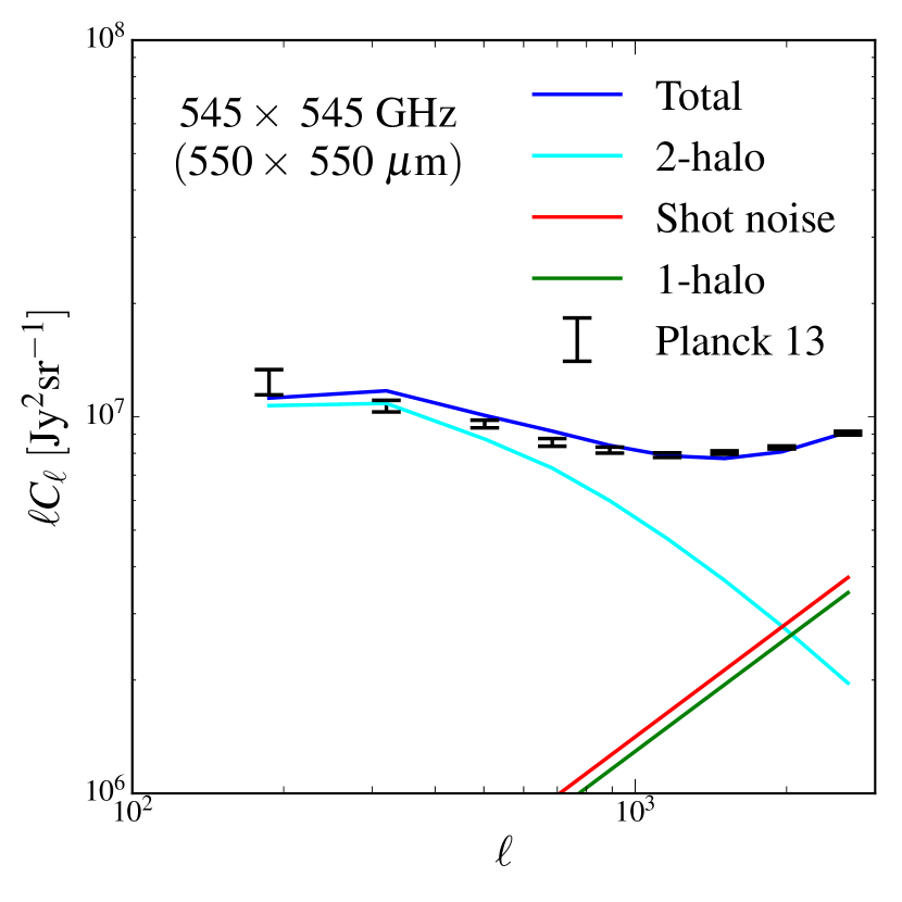
Figure 1: Model fit to the CFIRB angular power spectra measured by Planck Collaboration XXX (2014). The blue curve is our model, which is broken down into the 2-halo term (cyan), the shot noise (red), and the 1-halo term (green). See Fig. 16 for the auto and cross power spectra for four frequency bands.

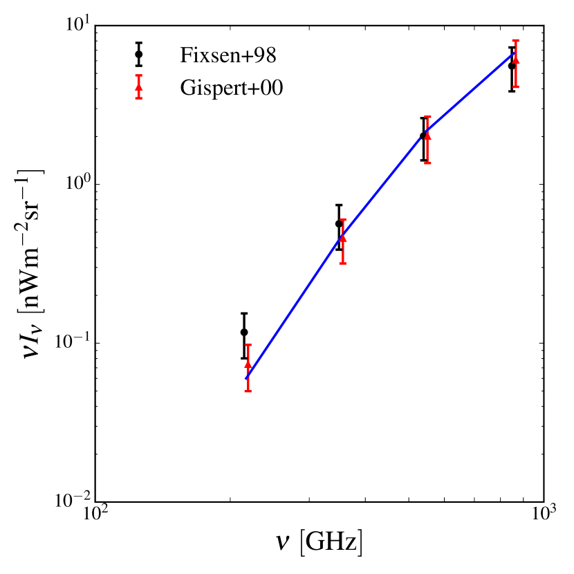
Figure 2: Prediction of the CFIRB intensity from our model compared with the measurement of COBE-FIRAS (Fixsen et al., 1998; Gispert et al., 2000). We use the four frequencies associated with the Planck-HFI bands. The blue curve presents our best-fitting model.

4.2 Fitting procedure

Our likelihood function $P({\bf D}|\theta)$ is given by

$$-\ln P({\bf D}|\theta)=\sum\frac{(D_{i}-M_{i}(\theta))^{2}}{\sigma_{i}^{2}}\ ,$$ (31)

where $D_{i}$ is a data point, $\sigma_{i}$ is its error bar, and $M_{i}$ is the model prediction based on a set of parameters $\theta$. For the CFIRB angular power spectra, $D_{i}$ is $C_{\ell}^{\nu\nu^{\prime}}$ and $\sigma_{i}$ is $\sigma(C_{\ell}^{\nu\nu^{\prime}})$ for four auto- and six cross- spectra, for $\ell$ between 187 and 2649.

We use the publicly available Markov chain Monte Carlo (MCMC) code emcee (Foreman-Mackey et al., 2013) version 2.0.0 to explore the parameter space. In particular, emcee uses an ensemble of $N$ walkers to update each other. Briefly, for a given walker at position $X_{k}$, the algorithm uses another walker $X_{j\neq k}$ to propose a new position $Y=X_{j}+Z[X_{k}-X_{j}]$, where $Z$ is a random variable drawn from a distribution function that makes the proposal symmetric. The new position is accepted with a probability of $\min\left(1,Z^{N-1}p(Y)/p(X_{k})\right)$, where $p(x)$ is the posterior probability. We refer the readers to Foreman-Mackey et al. (2013) for the complete description of the algorithm.

We have six free parameters in the gas regulator model (see Table 3), 87 data points, and the $\chi^{2}$ is $207.691$ for $81$ degrees of freedom. We use top-hat priors with generous ranges for all parameters. We have run 10 MCMC chains, each of which includes approximately 200,000 samples. We discard the first half of the chains as burn-in. We then apply the Gelman–Rubin diagnostic (Gelman & Rubin, 1992), which compares the “within-chain variance” and the “between-chain variance” for multiple chains. We have ensured that the scale reduction factor $\sqrt{\hat{R}}$ is much less than 1.1. Table 3 shows the constraints on the model parameters, and Table 4 shows the correlation matrix for these parameters. Fig. 13 shows the posterior distributions from the MCMC chains.

Our best-fitting $\chi^{2}$ is larger than that in Planck Collaboration XXX (2014), which is 100.7 for 98 degrees of freedom, including the 3000 GHz data and using free parameters to model the shot noise. Here we model the shot noise self-consistently but was unable to achieve such small $\chi^{2}$; therefore, our model should be regarded as qualitative rather than quantitative.

Parameter	Prior	Constraint (68%)	Definition	Equation
$\eta_{0}$	$[0.00,2.00]$	$1.08^{+0.07}_{-0.07}$	Minimum value of mass-loading factor (at $M_{\rm pk}$)	16
$\alpha_{1}$	$[0.00,3.00]$	$2.50^{+0.11}_{-0.07}$	Slope of mass-loading factor for low-mass end ($\eta\propto M^{-\alpha_{1}}$)	16
$\alpha_{2}$	$[0.00,3.00]$	$0.49^{+0.01}_{-0.01}$	Slope of mass-loading factor for high-mass end ($\eta\propto M^{\alpha_{2}}$)	16
$\beta$	$[1.50,2.50]$	$2.11^{+0.02}_{-0.02}$	Spectral index for dust opacity	14
$\sigma$	$[0.20,2.00]$	$0.35^{+0.04}_{-0.03}$	Logarithmic scatter of $L_{\rm IR}$ at a given halo mass	26
$\delta$	$[-1.00,3.00]$	$1.13^{+0.06}_{-0.06}$	Extra redshift dependence of accretion rate	9

Table 3: Constraints on the model parameters.

4.3 Best-fitting model

Fig. 1 shows the data and the best-fitting model (with the maximum likelihood) for the CFIRB the angular power spectrum at 545 GHz (550 $\micron$). Fig. 16 shows the full 10 auto- and cross-spectra from the four bands of Planck. We demonstrate the contribution from the 2-halo term, 1-halo term, and the shot noise. For the angular scale measured by Planck, the 1-halo term is sub-dominant. In Fig. 16, we can see that the agreement is good for almost all angular scales and all bands. The fit for the 217 GHz (1382 $\micron$) auto-power spectrum is noticeably worse than other frequencies, which could be caused by our simplistic assumption of SED. We note that this band is dominated by CMB at all scales, and that the power spectrum can be affected by the procedure used for removing CMB.

Fig. 2 shows the CFIRB intensity calculated from the best-fitting model. We show the data from both Fixsen et al. (1998) and Gispert et al. (2000), using the values and error bars quoted in table 5 in Planck Collaboration XVIII (2011). Our best-fitting model agrees better with Gispert et al. (2000), and we note that the result from Planck Collaboration XVIII (2011, see their fig. 15) also agrees better with Gispert et al. (2000).

4.4 Constraints on model parameters

In the following we discuss the implications of the constraints for our model parameters. We quote the median and the 68% constraints for the 1-D marginalized posterior distribution. Table 3 lists the parameter constraints.

• $\eta_{0}$ (minimum of the mass-loading factor, which occurs at $M_{\rm pk}$). The constraint is $1.08^{+0.07}_{-0.07}$. As mentioned in Section 2.3, several observations provided a lower limit for the mass-loading factor but the observed values are inconclusive.

• $\alpha_{1}$ (the slope of the mass-loading factor at low-mass end): The constraint is $2.50^{+0.11}_{-0.07}$, which implies $\eta\propto M_{\rm h}^{-2.50}\propto V_{\rm vir}^{-7.5}$. This scaling is much steeper compared with any of the supernova wind models. Our model prefers a very low $L_{\rm IR}$ for low-mass haloes, which can be related to low SFR and/or low dust content. It has been shown that low-mass haloes tend to have a $L_{\rm IR}$ lower than expected from the SFR due to the low mass content (e.g., Hayward et al., 2014).

• $\alpha_{2}$ (the slope of the mass-loading factor at high-mass end): The constraint is $0.49^{+0.01}_{-0.01}$. As it is less than 1.1, the SFR does not decrease at the high-mass end (see equation 4 and Fig. 8). We will further discuss this trend in Section 6.1.

• $\beta$ (slope of opacity, emissivity index): The constraint is $2.11^{+0.02}_{-0.02}$, which is close to the value $\beta=2$ expected from theory (Draine & Lee, 1984). It is higher than the results in Planck Collaboration XXX (2014, $\beta$=1.75) and the nearby late-type galaxies observed by Herschel in Boselli et al. (2012, $\beta$=1.5).

• $\sigma$ (scatter of ${\rm ln}S_{\nu}$ and $\ln L_{\rm IR}$ at a given halo mass): The constraint is $0.35^{+0.04}_{-0.03}$ ($0.13$ dex). This parameter is constrained by the shot noise; as we will see later, it also reproduces the bright-end of the IR luminosity functions (Fig. 4). We note that this scatter is smaller than our current knowledge of SFR. For example, the scatter between stellar mass and halo mass is estimated to be 0.2 dex (e.g., Reddick et al., 2013), and the scatter between SFR and stellar mass is estimated to be 0.15 dex (e.g., Bernhard et al., 2014); summing these two scatter values in quadrature will lead to a scatter of 0.25 dex between SFR and halo mass.

• $\delta$ (extra redshift dependence, equation 9): The constraints is $1.13^{+0.06}_{-0.06}$. This value deviates from zero, indicating that the dark matter accretion rate (equation 8) is insufficient to account for the full evolution of the SFR–mass relation. Our overall redshift dependence is approximately $(1+z)^{3.6}$ (see equation 35 below), which is consistent with the results of Planck Collaboration XXX (2014).

4.5 Summary of our model

Here we summarize the main scaling relations based on our parameter constraints. The $L_{\rm IR}$–mass relations is given by

$$L_{\rm IR}(M,z)=\frac{3.6\times 10^{10}}{1+2f(M)}\left(\frac{M}{10^{12}}\right)^{1.1}g(z)\ \rm L_{\odot}\ .$$ (32)

The dust mass is given by

$$M_{\rm d}(M,z)=\frac{14\times 10^{6}}{\left(1+2f(M)\right)^{2}}\left(\frac{M}{10^{12}}\right)^{1.1}\left(\frac{t}{{\rm Gyr}}\right)g(z)\ \rm M_{\odot}\ ,$$ (33)

and the dust temperature is given by

$$T_{\rm d}(M,z)=28\left(\frac{1+2f(M)}{t/{\rm Gyr}}\right)^{1/(4+\beta)}\ {\rm K}\ .$$ (34)

In the equations above, the extra time dependence is given by

$$g(z)=(1+1.11z)\sqrt{\Omega_{M}(1+z)^{3}+\Omega_{\Lambda}}(1+z)^{\delta}\ .$$ (35)

The extra mass dependence is given by

$$f(M)=f(x,y)=1+x+y-(1+x^{-1}+y^{-1})^{-1}\ ,$$ (36)

where

$$x=\left(\frac{M}{10^{12}}\right)^{-2.50}\ ,\quad y=\left(\frac{M}{10^{12}}\right)^{0.49}\ .$$ (37)

In addition, $t$ is the cosmic time

$$t=14.6\int_{z}^{\infty}\frac{dz^{\prime}}{(1+z^{\prime})\sqrt{\Omega_{M}(1+z^{\prime})^{3}+\Omega_{\Lambda}}}\ {\rm Gyr}\ .$$ (38)

Alternatively, one can use the fitting formula given in DM14, which is sufficiently accurate for $z>1$,

$$t=17.5(1+z)^{-1.5}\ {\rm Gyr}\ .$$ (39)

5 Comparisons with other observations

We now compare our model predictions with other observations. We choose not to fit all observations simultaneously because of the different sources of systematic errors involved in them. In all the following calculations, we use 1% of our MCMC chains to calculate the model predictions, and we plot the median as well as the 68% and 95% intervals for all quantities. In the main text, we only show the results of a single band or redshift bin for demonstration; the full comparisons can be found in Appendix B. This section focuses on direct observations from FIR/submillimetre surveys, including power spectra, number counts, and luminosity functions, while Section 6 focuses on derived quantities.

5.1 Correlation between CFIRB and CMB lensing potential

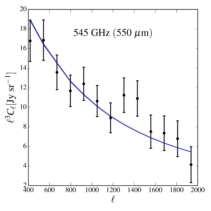
Figure 3: Correlation between CFIRB and CMB lensing potential. The blue band is the prediction from our model, while the data points are from Planck Collaboration XVIII (2014, see Fig. 18 for all Planck-HFI bands).

Planck Collaboration XVIII (2014) presented the first detection of the correlation between CFIRB and CMB lensing potential. The CMB lensing potential is dominated by haloes at $1\lesssim z\lesssim 3$ and is probed by the lower frequency bands of Planck (70 – 217 GHz), while the CFIRB redshift distribution peaks at $1\lesssim z\lesssim 2$ and is measured by the higher frequency bands of Planck. Therefore, the correlation between the two provides a powerful probe for the connection between dark matter and galaxies, as well as cross-check for systematics.

The cross power spectrum between the CMB lensing potential and CFIRB is given by

$$C_{\ell}^{\phi\nu}=\int_{0}^{\chi_{*}}B_{\nu}(z)\frac{3}{\ell^{2}}\Omega_{M}H_{0}^{2}\left(\frac{\chi_{*}-\chi}{\chi_{*}\chi}\right)P_{\rm lin}\left(k=\frac{\ell}{\chi},z\right)d\chi\ ,$$ (40)

where $\chi_{*}$ is the comoving distance to the last scattering surface, and $B_{\nu}(z)$ is given by equation (22) and is equivalent to $b_{\rm eff}(z)j_{\nu}(z)$.

Figs. 3 and 18 show that our model can recover the measurements presented in Planck Collaboration XVIII (2014). We note that the 68% and 95% intervals are very small because our model is constrained by the CFIRB spectra, which have much smaller error bars. Assuming that the IR luminosity is independent of halo mass, Planck Collaboration XVIII (2014) applied a halo occupation distribution model and found that $\rm log_{10}(M_{\rm min}/\rm M_{\odot})=10.5\pm 0.6$, where $M_{\rm min}$ is the minimum mass of a halo that hosts a central galaxy. Planck Collaboration XVIII (2014) interpreted this mass scale as the characteristic mass for haloes hosting CFIRB sources; however, as we will see below in Section 6.2 and Fig. 9, the effective galaxy bias consistent with this data set (as well as the CFIRB auto-correlation) corresponds to a halo mass of $10^{12.5}\ \rm M_{\odot}$ due to the mass dependence of SFR.

5.2 Bolometric infrared luminosity Functions

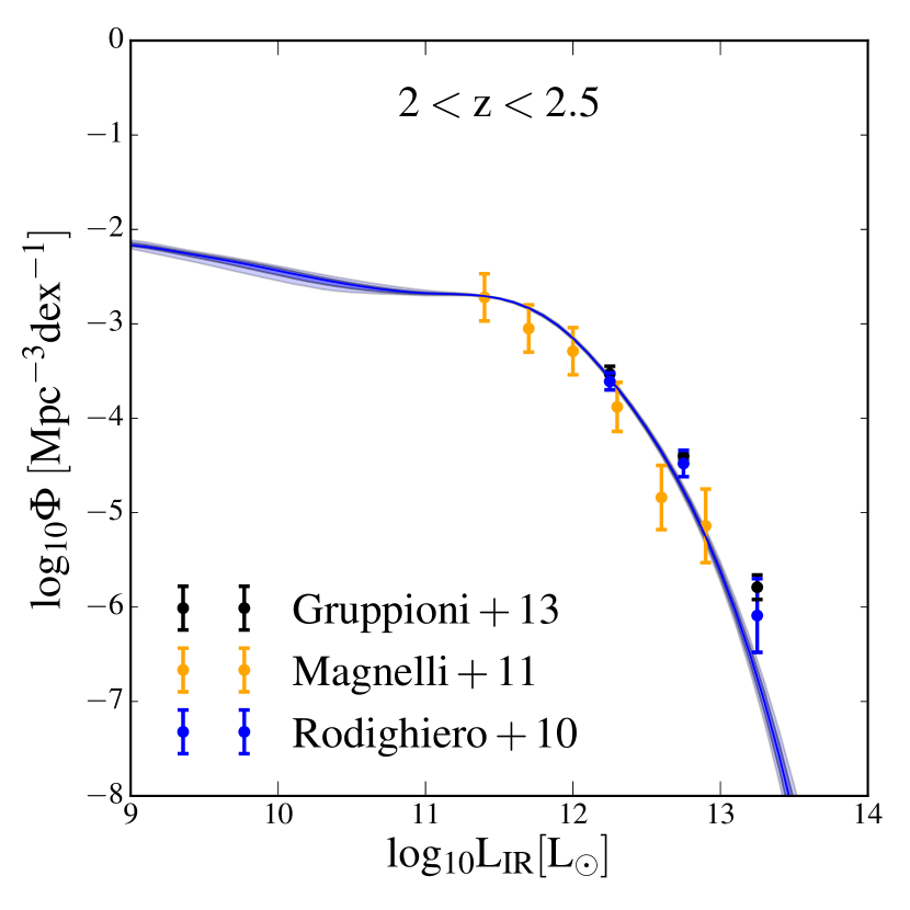
Figure 4: Bolometric infrared luminosity functions (8–1000µm). The observational data sets include Gruppioni et al. (2013) from Herschel, as well as Magnelli et al. (2011) and Rodighiero et al. (2010) from Spitzer (see Fig. 20 for multiple redshift bins between $z=0$ and 4).

We assume that at a given $M$ and $z$, the natural logarithm of the IR luminosity (${\rm ln}L$) of galaxy follows a normal distribution similar to ${\rm ln}S_{\nu}$,

$$P({\rm ln}L|M)=\frac{1}{\sqrt{2{\rm\pi}}\sigma}\exp\bigg{[}-\frac{\big{(}{\rm ln}L-\left\langle{{\rm ln}L}\right\rangle\big{)}^{2}}{2\sigma^{2}}\bigg{]}\ .$$ (41)

Here $\sigma$ is the same as in equation (26). The luminosity function is given by

$$\frac{dn}{d{\rm ln}L}(z)=\int dM\frac{dn}{dM}P({\rm ln}L|M)\ .$$ (42)

We compare our model with the bolometric IR luminosity functions (integrating over 8–1000µm) from the following publications:

• Gruppioni et al. (2013, table 6 therein) based on Herschel (70–550 $\micron$), $0<z<4.2$. The galaxies are selected from PACS (70, 100, 160 µm), and the SEDs are calibrated using SPIRE (250, 350, 550 $\micron$).

• Magnelli et al. (2011, table A6 therein) based on Spitzer (24 and 70 $\micron$), $1.3<z<2.3$. They performed stacked analyses and derived the SED using the correlation between the luminosities at 24 and 70 µm.

• Rodighiero et al. (2010, table 5 therein) based on Spitzer (8–24 $\micron$), $0<z<2.5$. The SED was derived using luminosities from optical to 24 $\micron$ and was thus not probing the peak of the dust emission. Nevertheless, their results are consistent with the results from Gruppioni et al. (2013) based on longer wavelengths.

• Le Floc’h et al. (2005, table 2 therein) based on Spitzer 8 µm, $0.3<z<1.2$. The bolometric luminosity was inferred from 24 $\micron$.

Fig. 4 shows the bolometric IR luminosity functions predicted from our model (see Fig. 20 for 11 redshift bins up to $z=4$). Since these data sets are based on slightly different redshift bins; we re-group these data points using the redshift bins in Gruppioni et al. (2013) and compute the model at the middle of the bin. We note that all these observations are based on mid-infrared and use various SED templates to calculate the bolometric IR luminosity; therefore, they can suffer from different statistical and systematic uncertainties and do not necessarily agree with other. Therefore, we also expect that they will not necessarily agree with our model constrained by CFIRB. As can be seen in Fig. 4, our model agrees with most of the data points but slightly under-predicts the bright end at high redshift. The scatter of the IR luminosity at a given mass ($\sigma$ in equation 26), as constrained by CFIRB, determines the bright-end slopes of the IR luminosity functions.

5.3 Number counts of FIR galaxies

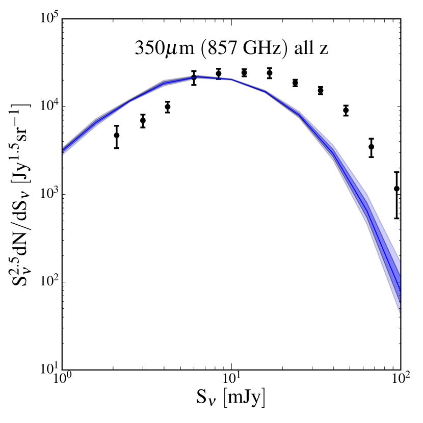
Figure 5: Number counts of infrared galaxies. The data points are from Béthermin et al. (2012) based on Herschel-SPIRE. Our model under-predicts the bright source counts while over-predicts the faint source counts for all redshifts (see Fig. 21 for all Herschel-SPIRE bands and several redshift bins).

The number counts, also known as the flux density distribution function of infrared sources, is given by

$$\frac{dN}{dS_{\nu}}(z_{1}<z<z_{2})=\int_{z_{1}}^{z_{2}}dz\chi^{2}\frac{d\chi}{dz}\frac{dn}{dS_{\nu}}\ .$$ (43)

We compare our model with the deep number counts measured by Béthermin et al. (2012) in the HerMES programme. These authors used the maps in 250, 350, and 500 $\micron$ in the COSMOS and GOODS-N fields observed by Herschel-SPIRE, and they used the catalogues of Spitzer 24 $\micron$ as priors for positions, flux densities, and redshifts. They provided the resolved number counts for $>$ 20 mJy and stacked number counts for between 2 and 20 mJy for several redshift bins.

Fig. 5 shows the comparison between our model (blue band) with the data points from Béthermin et al. (2012); the full comparison is presented in Fig. 21. Our model under-predicts the number of bright sources and over-predicts the number of faint sources. We note that our model includes neither starburst galaxies nor strongly lensed galaxies, which can contribute to the bright end of the number counts functions. We also note that recently Béthermin et al. (2017) show that the bright end of the number counts can be overestimated due to limited resolutions of the telescopes.

5.4 Redshift distribution of CFIRB

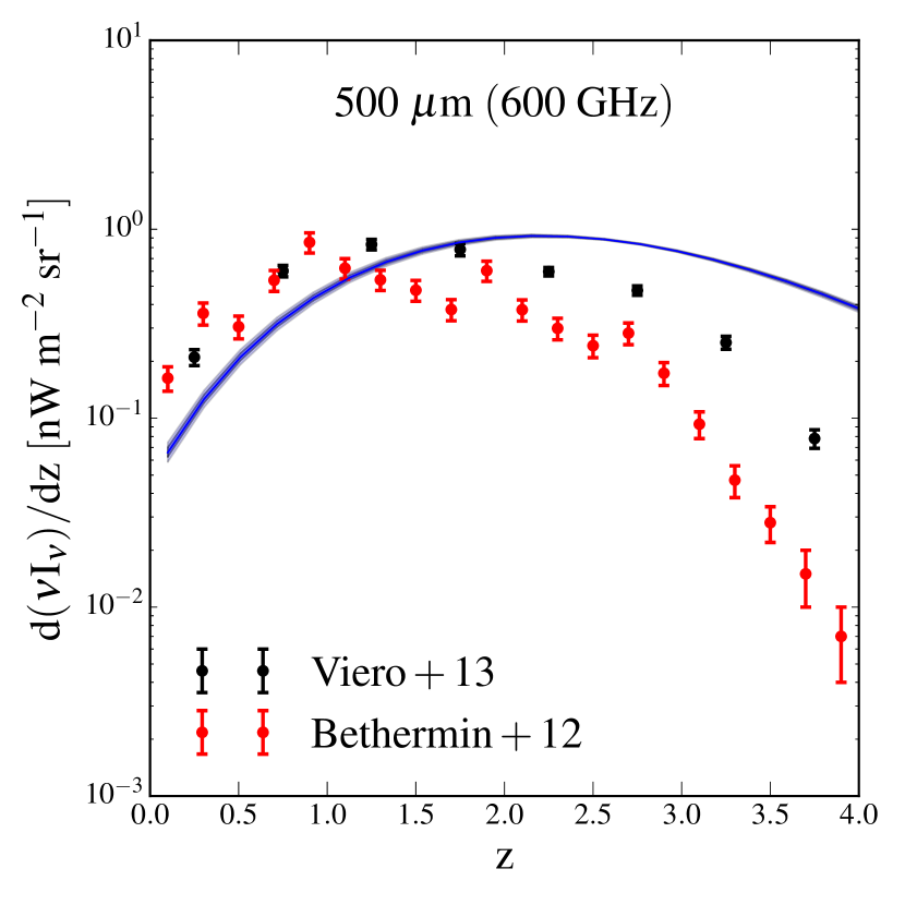
Figure 6: Redshift distribution of CFIRB emission. The data points are from resolved sources in Viero et al. (2013b, black points, based on optical) and Béthermin et al. (2012, red points, based on 24 $\micron$), which serve as lower limits. Our model is above the data points for $z>1.5$ but is slightly lower for $z<1$ (see Fig. 19 for all bands of Herschel–SPIRE).

The redshift distribution of CFIRB emission is given by

$$\frac{dI_{\nu}}{dz}=\chi^{2}\frac{d\chi}{dz}\int dS_{\nu}\frac{dn}{dS_{\nu}}S_{\nu}$$ (44)

We again compare our model with the data set from Béthermin et al. (2012), which was discussed in the previous section.

Independently, Viero et al. (2013b) conducted a stacking analysis to quantify the fraction of CFIRB from galaxies resolved in optical. Specifically, they used the optical galaxy catalogue from the Ultra-Deep Survey fields from the UKIRT Infrared Deep Survey. Using the galaxy positions and photometric redshift, they performed stacking analyses on FIR maps, including the 250, 350, and 500 $\micron$ data from Herschel-SPIRE, and the 1100 $\micron$ data from AzTEC. With this analysis, they were able to separate the contribution of CFIRB from star-forming and quiescent galaxies in different stellar mass and redshift ranges. Their sample resolves 80%, 69%, 65%, and 45% of CFIRB in 250, 350, 500, and 1100 $\micron$, respectively. As mentioned in Viero et al. (2013b), these measurements should be considered as lower limits, since optical catalogues can miss galaxies in FIR, either due to heavy dust obscuration or low intrinsic luminosity. The completeness also decreases rapidly with redshift. Viero et al. (2013b) also suggested that such measurements provide an effective way to break the degeneracies between redshift distribution, temperature, and halo bias.

Figs. 6 and 19 present the comparison between the redshift distribution of CFIRB from our model (blue band) and the results in Béthermin et al. (2012, red points) and Viero et al. (2013b, black points). Our model predicts higher differential intensity for $z>2$ than the data points, which should be considered as lower limits. If we use a lower differential intensity that is consistent with the data points, we will underestimate the total CFIRB intensity and clustering. On the other hand, our model predicts slightly lower differential intensity for $z<1$. This is consistent with what we saw in Fig. 5, where our model also under-predicts the number counts for $z<2$ observed by Herschel.

5.5 CFIRB power spectrum from Herschel

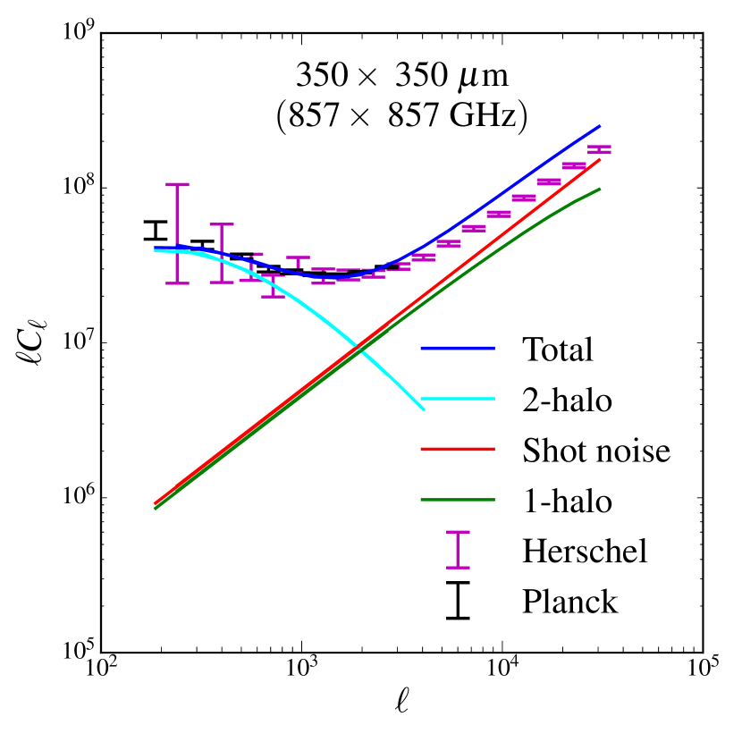
Figure 7: Comparison between our model and the power spectra from Herschel published in Viero et al. (2013a). Our model constrained by Planck overproduces the small-scale power when compared with Herschel. We show the power spectra of both Planck and Herschel in their common frequency 857 GHz (350 $\micron$) to illustrate the different angular scale and sizes of error bars (see Fig. 17 for all frequencies for Herschel-SPIRE).

Fig. 7 shows the CFIRB power spectrum at 350 $\micron$ measured by Herschel (Viero et al., 2013a), compared with our model and the measurement of Planck in the same band. Fig. 17 shows the comparison between our model and all frequencies of Herschel-SPIRE. The power spectra are based on the HerMES program, which covers 70 $\rm deg^{2}$ in 250, 350, and 500 $\micron$. The galactic cirrus was removed using the 100 $\micron$ maps from IRAS. Compared with the Planck data, the Herschel power spectra extend to smaller angular scales. As can be seen, our model over-predict the power for $\ell\gtrsim 4000$. The sum of the shot noise (red) and the 1-halo term (green) exceeds the data points. That is, the Planck power spectra favour higher clustering at small scales. Since the Planck power spectra has limited constraining power on small scale, extrapolating our results to small scales leads to this inconsistency with Herschel results.

6 Implications of our model

Based on the constraints on parameters, we calculate various properties of dusty star-forming galaxies and compare them with observations.

6.1 IR luminosity–mass relation

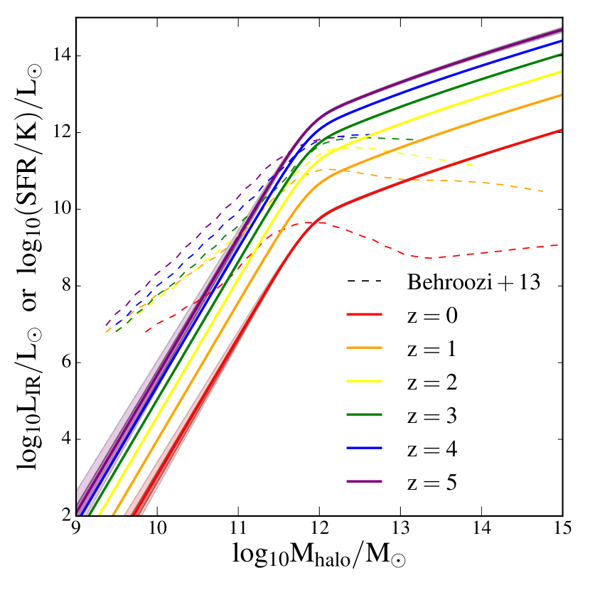
Figure 8: Infrared luminosity versus halo mass in our model (solid curves); the function is provided in equation (32). Comparing with the SFR constraints from UV/optical from Behroozi et al. (2013, dash curves) and assuming $L_{\rm IR}={\rm SFR}/K$, we find that the $L_{\rm IR}$ at low-mass end is lower than expected from SFR, while the high-mass end requires higher $L_{\rm IR}$ than expected from SFR.

Fig. 8 shows the mean relation between the infrared luminosity and the halo mass constrained by CFIRB (equation 32). The solid curves correspond to our model at various redshifts. The dash curves show the $L_{\rm IR}$–$M_{\rm h}$ relation expected from the SFR from Behroozi et al. (2013) and $L_{\rm IR}={\rm SFR}/K$.

For low-mass haloes, $L_{\rm IR}$ is lower than the expectation from SFR. These low-mass haloes tend to be have low dust mass and thus lower IR luminosity given their SFR. For example, using hydrodynamic simulations with radiative transfer, Hayward et al. (2014) have shown that low-mass galaxies are inefficient in absorbing UV photons, and inferring SFR from the IR luminosity can significantly underestimate the SFR for these galaxies (also see, e.g., Jonsson et al., 2006). Using the data from HerMES, Heinis et al. (2014) have found that galaxies with low stellar mass have lower dust attenuation, as well as lower IR excess (the ratio between $L_{\rm IR}$ and $L_{\rm UV}$); this confirms the findings in simulations that low-mass galaxies are inefficient in absorbing UV photons. Therefore, when converting SFR to $L_{\rm IR}$, one should consider the mass dependence of dust attenuation. In Wu & Doré (2017a), we show that a mass-dependent dust attenuation is crucial for recovering the observed CFIRB intensity and amplitude.

For massive haloes, the IR luminosity is significantly higher than what we expect from SFR. The CFIRB power spectra indicate a rather high galaxy bias that requires the contribution of FIR photons from massive haloes (see Section 6.2 below). If we use the $L_{\rm IR}$–$M_{\rm h}$ relation from Behroozi et al. (2013) in our halo model to calculate the power spectra, the amplitude of the CFIRB power spectra are too low regardless of the dust temperature used.

We note that, in addition to massive young stars, old stars can also heat the dust and contribute to FIR emission (e.g., Groves et al., 2012; Fumagalli et al., 2014; Utomo et al., 2014). For example, using hydrodynamic simulations with radiative transfer, Narayanan et al. (2015) have found that old stars can contribute to up to half of the IR luminosity. In addition, the heating from old stars contributes to a larger fraction of the IR luminosity for quiescent galaxies than for star-forming galaxies (e.g., Fumagalli et al., 2014). Since these massive haloes tend to host quiescent galaxies, we expect that the contribution of heating from old stars is significant.

On the other hand, dust-obscured AGN can also heat the dust and contribute the FIR emissions (e.g., Alexander et al., 2005; Lutz et al., 2005; Yan et al., 2005; Le Floc’h et al., 2007; Sajina et al., 2012). However, the contribution from AGNs are expected to be low for massive galaxies; it has been shown that luminous AGNs are hosted by haloes of mass $10^{12}-10^{13}\ \rm M_{\odot}$ (e.g., Alexander & Hickox, 2012). Therefore, AGNs are unlikely to be the main sources of the excess FIR emission.

The excess of FIR light for massive haloes has also be seen in previous publications. For example, Clements et al. (2014) matched Planck sources and HerMES survey from Herschel and found four clumps consistent with galaxy clusters at $0.8<z<2.3$. They found that these cluster-like clumps have $L_{\rm IR}=3-70\times 10^{12}\ \rm L_{\odot}$; if one assumes that all the IR emissions are associated with star formation, such IR luminosities would imply an SFR of $600-10^{4}\rm M_{\odot}yr^{-1}$. Narayanan et al. (2015) used hydrodynamic simulations with radiative transfer to show that at $z\approx 2-3$, a dark matter halo of $10^{13}\rm M_{\odot}$ can have very high SFR ($500-1000\rm M_{\odot}yr^{-1}$). Such haloes can host groups of galaxies that are bright in submillimetre for a prolonged period due to constant gas infall. These findings suggest that there can indeed be IR-bright galaxies in massive haloes, which contribute the strong galaxy bias we find for CFIRB.

6.2 Effective bias

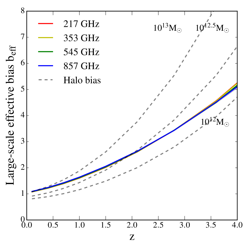
Figure 9: The effective bias from our model, which is consistent with halo mass $10^{13}\rm M_{\odot}$ at $z=0$ and $10^{12.5}\rm M_{\odot}$ at $z=2$.

Fig. 9 shows the large-scale effective bias calculated from our model,

$$b_{\rm eff}=\frac{B_{\nu}(z)}{j_{\nu}(z)}\ ,$$ (45)

where ${B_{\nu}(z)}$ and ${j_{\nu}(z)}$ are given by equations (18) and (22). We note that since the SED depends on halo mass, the effective bias weakly depends on the frequency. For comparison, we show the bias of haloes of $M_{\rm h}=10^{12,12.5,13}\rm M_{\odot}$ as a function of redshift, using the fitting function from Tinker et al. (2010). As can be seen, our effective bias is consistent with haloes of mass $10^{13}\rm M_{\odot}$ at $z=0$ and $10^{12.5}\rm M_{\odot}$ at $z=2$. The CFIRB data favours a high galaxy bias and thus more contribution from haloes above $10^{12}\ \rm M_{\odot}$ .

An alternative explanation of this high galaxy bias could be that FIR galaxies represent biased environments, and the simple linear halo bias does not apply. It has been shown that the halo bias, in addition to its dependence on halo mass, can depend on formation time, concentration, and occupation (e.g. Wechsler et al., 2006). If FIR galaxies preferentially reside in haloes with recent major merger, or if the FIR luminosity and formation history are correlated, it might be possible to explain the high galaxy bias without invoking extra FIR sources in massive haloes. We will explore this in future work.

6.3 Global SFR density

Fig. 10 shows the SFR density based on our model,

$$\rho_{{\rm SFR}}(z)=K\int dM\frac{dn}{dM}L_{\rm IR}(M,z)\ ,$$ (46)

where $K$ is $1.7\times 10^{-10}\rm M_{\odot}yr^{-1}\rm L_{\odot}^{-1}$ (Kennicutt, 1998, assuming Salpeter initial mass function).

We fit the four-parameter function proposed in Madau & Dickinson (2014) to our $\rho_{{\rm SFR}}$ (also see Robertson et al., 2015)

$$\rho_{{\rm SFR}}(z)=a_{p}\frac{(1+z)^{b_{p}}}{1+[(1+z)/c_{p}]^{d_{p}}}{\rm M_{\odot}Mpc^{-3}yr^{-1}}$$ (47)

where

$$a_{p} =0.0157_{-0.0004}^{+0.0003}$$ (48)

$$b_{p} =2.51_{-0.03}^{+0.04}$$

$$c_{p} =3.64_{-0.05}^{+0.04}$$

$$d_{p} =5.46_{-0.09}^{+0.10}\ .$$

We note that these parameters are highly degenerate with each other.

For comparison, we plot the results based on UV and IR luminosity functions compiled by Madau & Dickinson (2014, table 1 and references therein). The green points correspond to the results from FUV luminosity function (1500Å) from GALEX and HST with corrections of dust attenuation. The red points correspond to the results from the IR luminosity function (8–1000µm) from IRAS, Spitzer, and Herschel. We note that Madau & Dickinson (2014) re-computed the total luminosity density by extrapolating the best-fitting luminosity functions down to $0.03L_{*}$ at each redshift from each publication. The faint-end slope and the dust extinction can therefore lead to significant uncertainties. They also cautioned that there is no robust measurements of SFR density for $z\gg 2$ due to the lack of robust selections. We also note that Robertson et al. (2015) found results very similar to Madau & Dickinson (2014) when they added a few more UV results, extrapolated the observed UV and IR luminosity functions down to lower luminosities, and included the constraints of the integrated Thompson optical depth from Planck Collaboration XVI (2014).

For $z<2$, our SFR agrees with the constraints from Madau & Dickinson (2014). For high redshift ($z>3$), CFIRB does not provide strong constraints on the SFR, and the result is the extrapolation from low redshift; however, it is higher than UV constraints. We note that the halo model in Planck Collaboration XXX (2014) also gave higher SFR density at high redshift, which could be related to their parametrization of redshift evolution (also see Serra et al., 2016). On the other hand, observations of gamma-ray bursts (e.g., Kistler et al., 2009) and UV background (e.g., Mitchell-Wynne et al., 2015) also hint at excess of SFR compared with the results from luminosity functions.

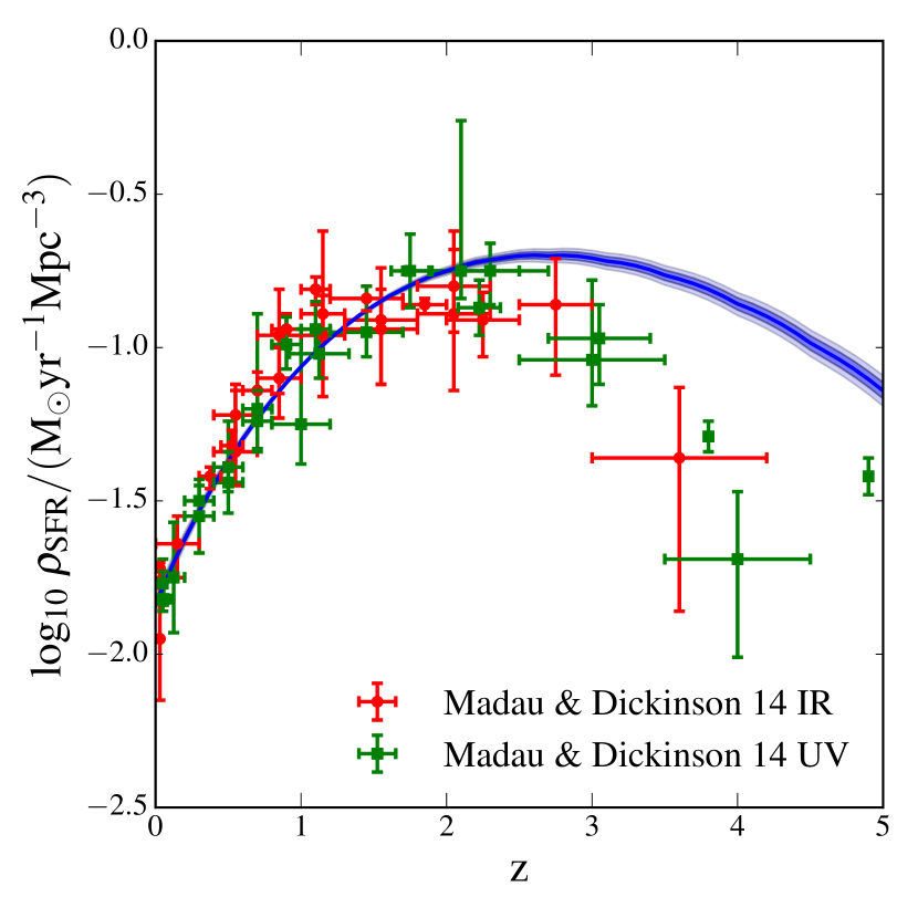
Figure 10: Cosmic SFR density inferred from our model (blue band). Our model is consistent with the results from Madau & Dickinson (2014, red and green points).

6.4 Cosmic dust mass density

Fig. 11 shows the cosmic dust mass density calculated from our model. The dust density is calculated by integrating over the halo mass function in physical units,

$$\rho_{\rm dust}(z)=\int dz\frac{dn}{dM}M_{\rm dust}(M,z)\ .$$ (49)

We express the dust mass density in unit of the critical density of the Universe,

$$\Omega_{\rm dust}(z)=\frac{\rho_{\rm dust}(z)}{\rho_{\rm crit}(z)}\ ,$$ (50)

where

$$\rho_{\rm crit}(z)=2.775\times 10^{11}h^{2}\bigg{(}\Omega_{M}(1+z)^{3}+\Omega_{\Lambda}\bigg{)}\rm{\rm M_{\odot}Mpc^{-3}}\ .$$ (51)

For $z>1$, our results are consistent with the results of Thacker et al. (2013) based on the CFIRB power spectra form H-ATLAS of Herschel. For $z<1$, our results are lower than Thacker et al. (2013) and the low-redshift results of Dunne et al. (2011), which were derived from the luminosity functions of H-ATLAS. This is related to the fact that our model predicts lower number counts than those observed by Herschel. For comparison, we include the results using Mg ii absorber from Ménard & Fukugita (2012). The dust mass density derived from Mg ii serves as a lower limit for the dust associated with galactic haloes; the dust associated with galactic discs has been shown to be comparable to the dust associated with galactic haloes (Fukugita & Peebles, 2004; Driver et al., 2007). Therefore, the total dust mass associated with galaxies is approximately twice of the values of the data points of Ménard & Fukugita (2012).

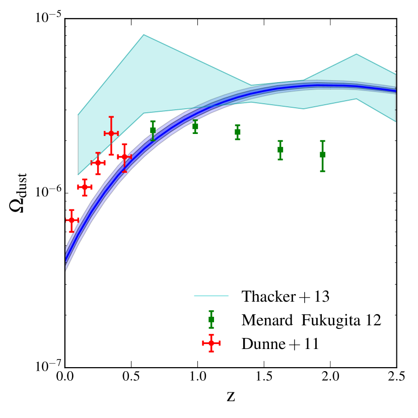
Figure 11: Cosmic dust mass density inferred from our model. Compared with the results from Thacker et al. (2013) using CFIRB of H-ATLAS and from Dunne et al. (2011) using the luminosity functions of H-ATLAS, our results are consistent at $z>1$ but are lower at $z<1$. We note that the results from Ménard & Fukugita (2012) using Mg ii absorbers serve as a lower limit of the dust in galactic haloes.

6.5 Dust temperature and mass

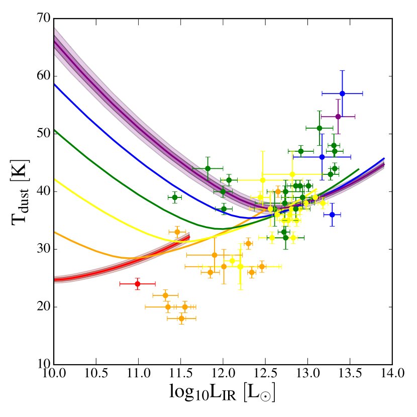
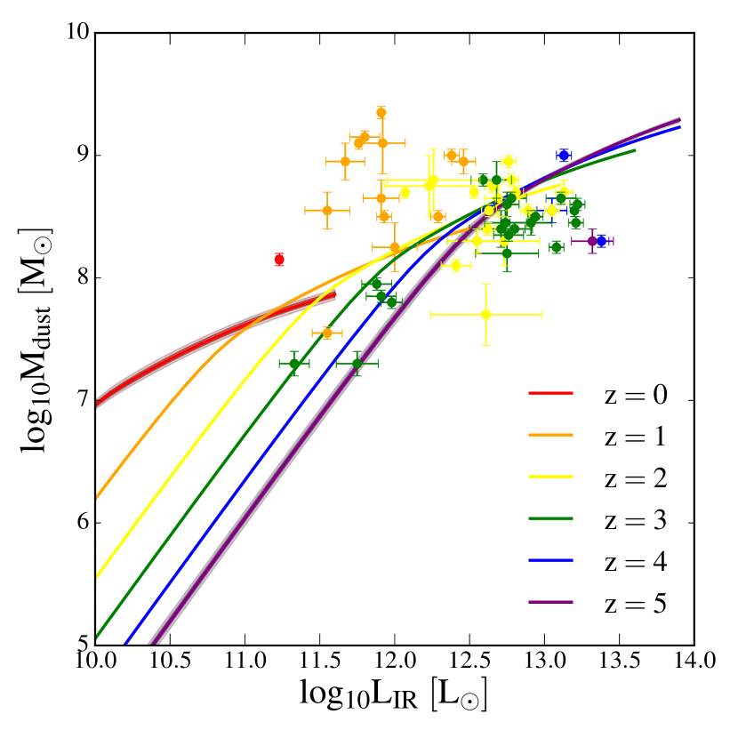
Figure 12: Dust properties from our model compared with observations of 61 SMGs observed by Herschel (Magnelli et al., 2012). We only show the the model uncertainties at $z$ = 0 and 5, and the uncertainties at other redshifts are very similar. We note that this figure is mainly for demonstrating the orders of magnitude because of the complex selection function involved. Left: Our model predicts higher dust temperature than the observation. Right: Our mean dust mass is slightly lower than the observation.

Fig. 12 shows the dust properties from our model. The left-/right- hand panel corresponds to dust temperature/mass versus IR luminosity at various redshifts, shown by different colours. Our model predicts non-monotonic relations with $L_{\rm IR}$; $M_{\rm d}$ tends to be low at both the bright and faint ends, while $T_{\rm d}$ tends to be high at both ends. This can be understood through the mass dependence of the mass-loading factor. In our model, the dust mass is given by

$$M_{\rm d}\propto\frac{1}{(1-R+\eta)^{2}}$$ (52)

(see equations 12 and 33). The high mass-loading factor for both high- and low-mass haloes leads to strong mass outflow and thus low dust mass. In addition, under the assumption of local thermal equilibrium, the dust temperature depends on the ratio between $L_{\rm IR}$ and $M_{\rm d}$,

$$T_{\rm d}\propto\bigg{(}\frac{L_{\rm IR}}{M_{\rm d}}\bigg{)}^{1/(4+\beta)}\propto({1-R+\eta})^{1/(4+\beta)}$$ (53)

(see equations 15 and 34). Therefore, at a given redshift, haloes at both high- and low-mass ends tend to have high dust temperature due to the high mass-loading factor.

We compare our results with the observational results in Magnelli et al. (2012, M12 thereafter), which include 61 submillimetre galaxies (SMGs) selected from ground-based observations and observed with PACS and SPIRE instruments onboard Herschel. We caution that this comparison is mainly for demonstrating the range of values, as the observations of SMGs tend to select merger-driven starbursts and has incomplete coverage for the main-sequence galaxies. As stated in M12, for high IR luminosity, the sample is representative of the entire SMG population, but these galaxies tend to be associated with merger-driven starbursts; on the other hand, for low IR luminosity, the sample tends to bias towards low redshift and colder dust. M12 concluded that approximately half of the sample is consistent with the merger-drive starbursts, while the other half is consistent with the main sequence of stellar mass and SFR. That is, this sample may not be relevant for the galaxies contributing to the CFIRB.

The left-hand panel of Fig. 12 shows the relation between $T_{\rm d}$ and $L_{\rm IR}$ predicted from our model. The correlation between $L_{\rm IR}$ and $T_{\rm d}$ has been known for SMGs (Chapman et al., 2005; Hwang et al., 2010; Hayward et al., 2012). In M12, $T_{\rm d}$ and $L_{\rm IR}$ are derived from fitting the SED to a modified blackbody with a single dust temperature, with $\beta=1.5$. We note that M12 used 40–120 $\micron$ to calculate $L_{\rm FIR}$ and assumed $L_{\rm IR}=1.91L_{\rm FIR}$. The dust temperature from M12 is lower than ours for $z<2$. This may reflect the SMG selection tends to bias towards low-redshift, low-temperature galaxies. In our model, the trend is reversed for faint galaxies; since we require strong feedback to suppress the SFR for low-mass haloes, this feedback also suppresses the dust mass and increases the dust temperature.

The right-hand panel of Fig. 12 shows the relation between $M_{\rm d}$ and $L_{\rm IR}$ from our model, as well as the measurements in M12. To derive the dust mass, M12 assumed a power-law distribution of dust temperature and fit the SED. Our model is consistent with M12. Nevertheless, M12 showed higher dust mass for $z<2$, and this difference is related to the lower dust temperature seen in the left-hand panel.

7 Discussion

In this work, we show that the gas regulator model provides a qualitative description for the CFIRB power spectra but is unable to produce all the details in observations. In this section, we discuss the limitations of our implementation of the gas regulator model and possible improvements.

In our implementation, we assume that most of the parameters are time-independent and mass-independent, and we incorporate the mass-dependence in the mass-loading factor (equation 16) and the extra time-dependence in SFR (equation 9). These parametrizations attempt to capture the effects of feedback, but they do not capture the detailed physics and thus cannot reproduce observations perfectly. The effective mass-loading factor $\eta$, the accretion of gas $f_{\rm ga}$ and stars ($1-f_{\rm ga}$), and the return fraction $R$ can all have non-trivial time and mass dependence. Capturing the time and mass dependence accurately would require hydrodynamic simulations or semi-analytic models. The limitations of the gas regulator model have also been demonstrated in the literature. For example, DM14 have shown that their fiducial model systematically under-estimates the specific SFR at $1<z<4$. In our work, we use a few free parameters but are still unable to fit the data perfectly.

Krumholz & Dekel (2012) implemented a metal-dependent SFR to take into account the fact that at high redshift, low-mass galaxies tend to have low metallicities and are unable to sustain a cool gas reservoir. Therefore, the SFR for low-metallicity galaxies is suppressed and is lower than what we would expect from the gas accretion rate. In our model, this effect is mimicked by the high effective mass-loading factor for low-mass galaxies. Our model qualitatively captures such trend; however, in principle, the SFR should be modelled self-consistently given the metallicity and dust.

Furthermore, in our model we assume that all galaxies follow a simple modified body SED with the dust temperature calculated by assuming thermal equilibrium. This assumption is too simplistic and may be the reason why we have significantly worse fit in the 217 GHz band.

Our model does not include starburst galaxies, which contribute to $\sim$10 per cent of the cosmic SFR density at $z\sim 2$ (Rodighiero et al., 2011; Sargent et al., 2012) and are expected to have negligible contribution to CFIRB (Shang et al., 2012; Béthermin et al., 2013). Including the starburst galaxies could increase the bright end of the luminosity functions and number counts. However, an extra component for starburst would boost the power spectrum in the same way as a higher gas accretion rate would, and breaking such degeneracy would require a joint fit to the bright end of the luminosity functions.

8 Summary

We apply the gas regulator model of galaxy evolution to describe dusty star-forming galaxies across cosmic time. We fit the model to the CFIRB power spectra observed by Planck. We compare our model predictions with the total CFIRB intensity measured by COBE, the correlation between CFIRB and CMB lensing potential measured by Planck, the bolometric IR luminosity functions up to $z=4$ from Herschel and Spitzer, and the total number counts from Herschel. The implications of our model are summarized as follows:

• The CFIRB power spectra favour a strong clustering of FIR galaxies. At $z=0$ ($z=2$), the large-scale galaxy bias is equivalent to the bias of dark matter haloes of mass $10^{13}$ ($10^{12.5}$) $\rm M_{\odot}$. This galaxy bias is consistent with the correlation between CFIRB and CMB lensing potential.

• The luminosity–mass relation from our model indicates that for massive haloes, the IR luminosity is higher than expected from the SFR constrained by UV and optical. This result is consistent with the high galaxy bias we have found. This excess in IR luminosity for massive haloes may come from the dust heated by old stellar populations.

• In our model, the luminosity–mass relation for low-mass haloes is lower than expected from the SFR constrained by UV and optical. These low-mass galaxies tend to be inefficient in absorbing UV photons, and their FIR emissions can underestimate the true SFR.

• Our model under-predicts the bright source counts of Herschel, slightly under-predicts the differential CFIRB intensity of Herschel for $z<1$, and over-predicts the CFIRB power spectra of Herschel at small scales.

• The cosmic star formation history from our model agrees with the recent compilation of Madau & Dickinson (2014) at $z<2$ but shows an excess at higher redshift. In addition, the total dust mass density across cosmic time is consistent with the results from Herschel CFIRB at $z>1$, while it is lower than the results from IR luminosity functions at $z<1$.

• Compared with SMGs selected from ground-based surveys, the galaxies in our model tend to have higher dust temperature ($T_{\rm dust}\gtrsim 25$ at $z=0$ and increases with redshift) and lower dust mass.

Our theoretical framework provides a simple, physically-motivated way to compare different FIR observations. It can be generalized to compute the foreground for various intensity mapping experiments. Our framework will also be useful for optimizing the survey designs and strategies for future FIR surveys. For example, the next generation CMB experiments, such as PIXIE (Kogut et al., 2011) and CORE (De Zotti et al., 2015), will provide larger frequency coverage and/or higher angular resolution and sensitivity than Planck and will be able to provide better measurements for the CFIRB anisotropies as well as individual sources. In Wu & Doré (2017b), we investigate the constraining power from future CFIRB experiments. The Far-IR Surveyor, which is currently explored by NASA, will reveal many more properties of dusty star-forming galaxies.

Appendix A Summary of parameters

Table 4 shows the correlation matrix of these parameters. Fig. 13 shows the 1-D and 2-D posterior distributions from the MCMC chains, which use the corner software (Foreman-Mackey, 2016).

Figs. 14 and 15 show the sensitivity of the power spectra to the model parameters at 217GHz and 857 GHz. In each panel, we increase or decrease a parameter by $2\sigma$. We note that the parameter $\sigma$ only affects the shot noise. Since shot noise dominates at larger $k$ and at higher frequency, the impacts of $\sigma$ is the strongest at large $k$ at 857 GHz.

	$\eta_{0}$	$\alpha_{1}$	$\alpha_{2}$	$\beta$	$\sigma$	$\delta$
$\eta_{0}$	1.00	-0.59	-0.88	-0.48	-0.07	0.99
$\alpha_{1}$	-0.59	1.00	0.55	0.36	-0.47	-0.53
$\alpha_{2}$	-0.88	0.55	1.00	0.50	0.26	-0.86
$\beta$	-0.48	0.36	0.50	1.00	-0.05	-0.56
$\sigma$	-0.07	-0.47	0.26	-0.05	1.00	-0.10
$\delta$	0.99	-0.53	-0.86	-0.56	-0.10	1.00

Table 4: Correlation matrix for the model parameters.

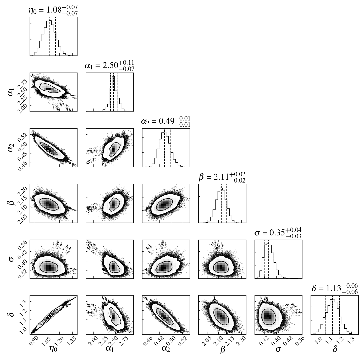
Figure 13: The 68% and 95% constraints of our model parameters. The diagonal panels show the posterior distribution and the 68% constraint of each parameter.

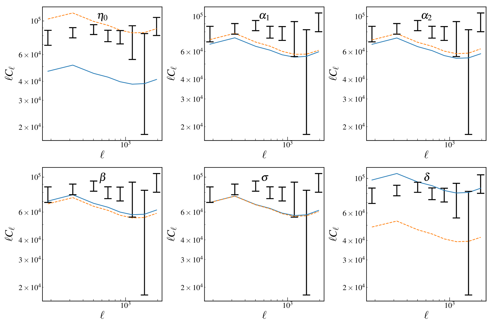
Figure 14: Sensitivity of angular power spectra (217 GHz) to model parameters. In each panel, the solid and dash curves correspond to increasing and decreasing the model parameters by $2\sigma$.

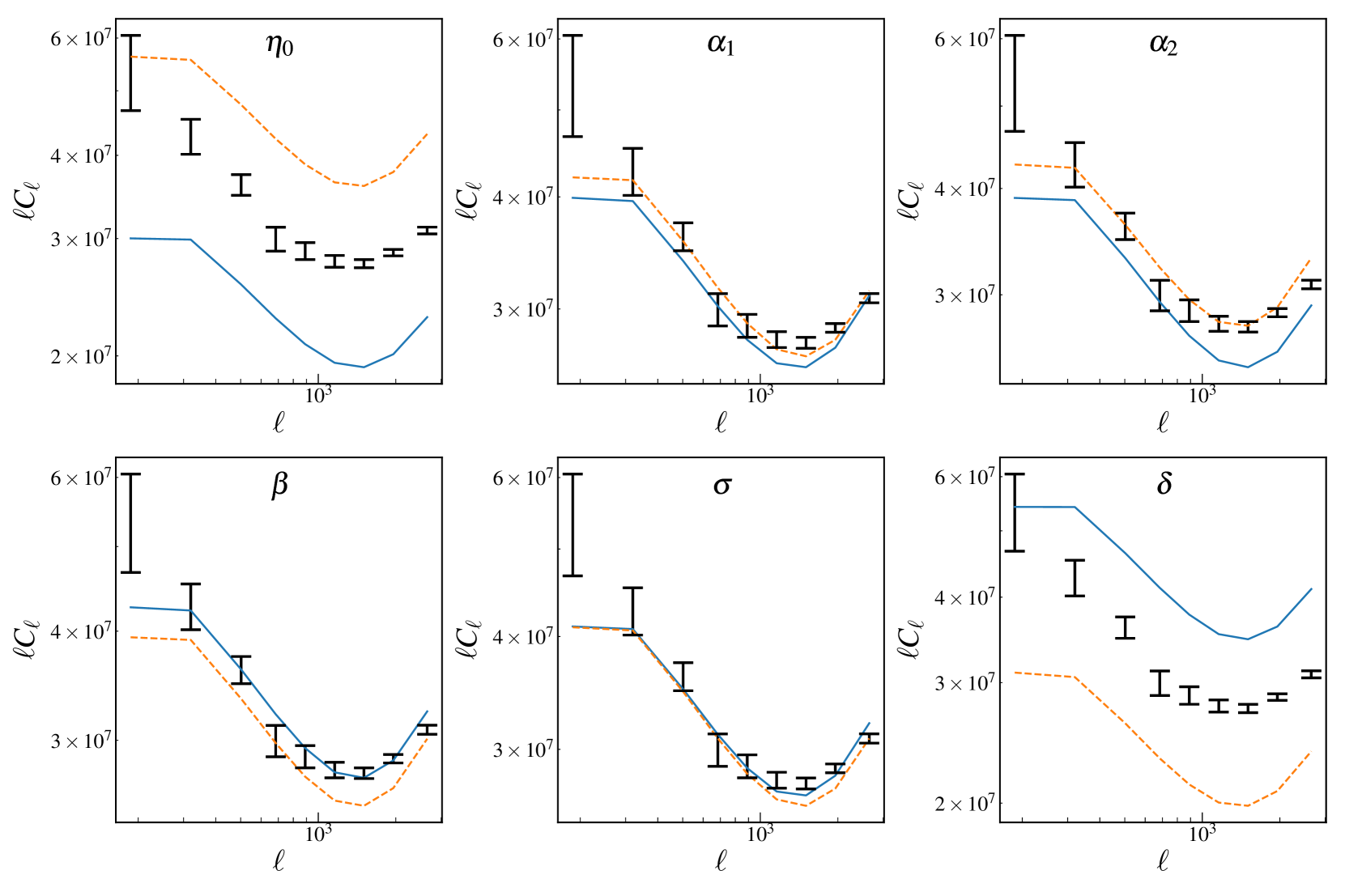
Figure 15: Same as Fig. 14 but for 857 GHz.

Appendix B Complete figures of comparisons between observations and our model

Most of the figures in the main text only show a single band or redshift slice for the purpose of demonstration. In this appendix, we show the full comparison between model predictions and observations we have conducted.

• Fig. 16: our fit to the Planck power spectra of CFIRB.

• Fig. 17: our model prediction for the Herschel power spectra of CFIRB.

• Fig. 18: our model prediction for the correlation between CFIRB and CMB lensing potential.

• Fig. 19: our model prediction for the redshift distribution of CFIRB emission.

• Fig. 20: our model prediction for the bolometric IR luminosity functions.

• Fig. 21: our model prediction for the FIR flux density functions (number counts).

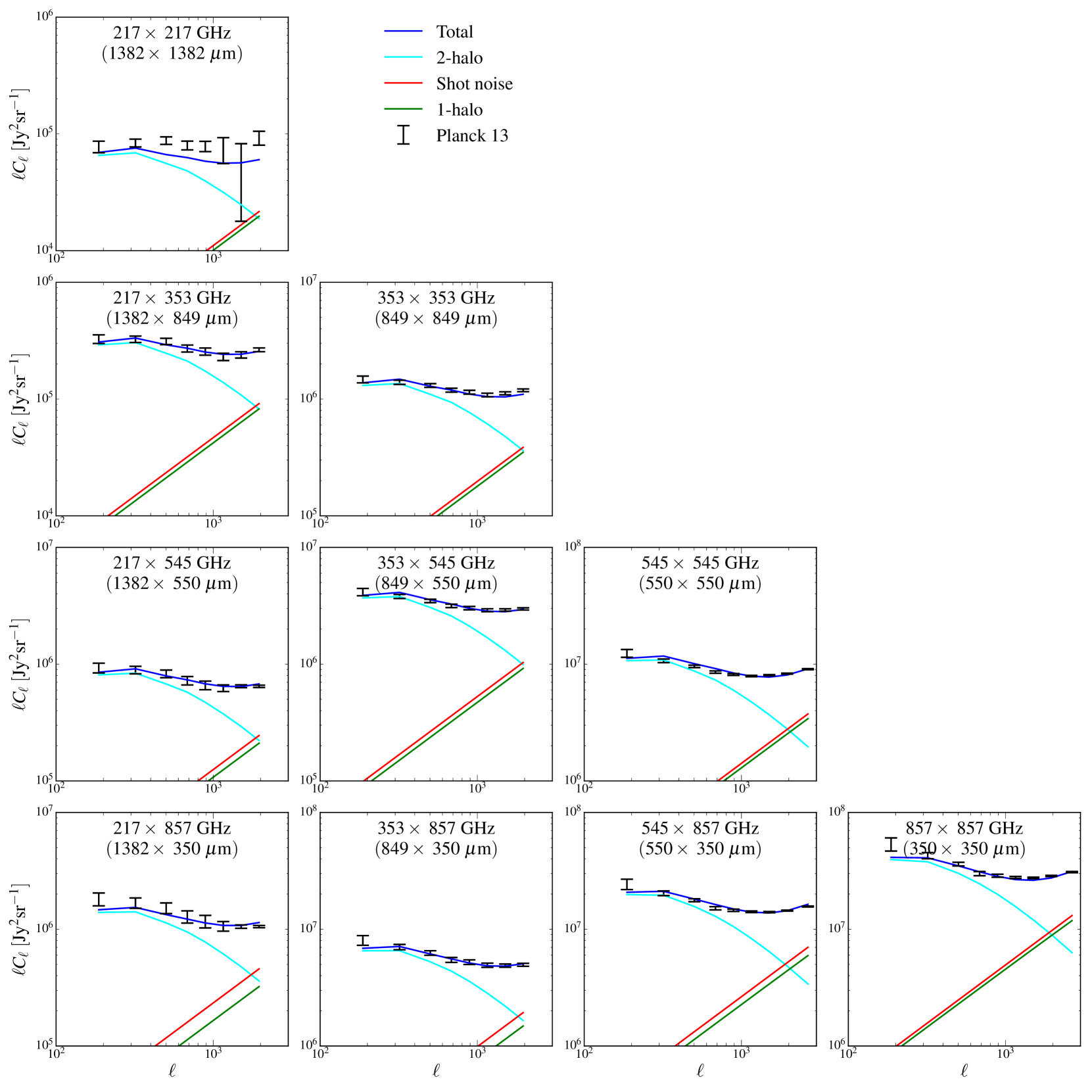
Figure 16: Our model fitting to the CFIRB power spectra from Planck.

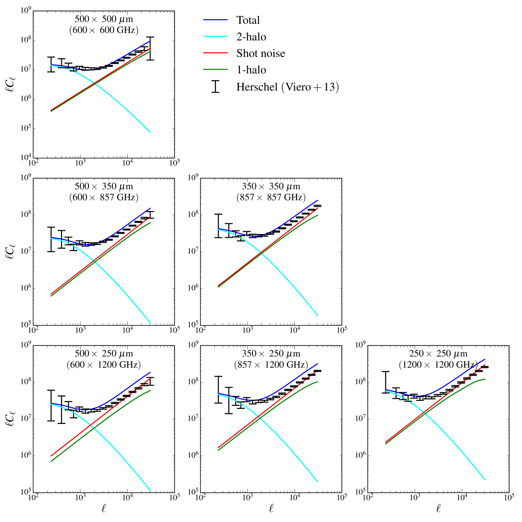
Figure 17: CFIRB power spectra from Herschel–SPIRE (see Section 5.5) compared with our model prediction.

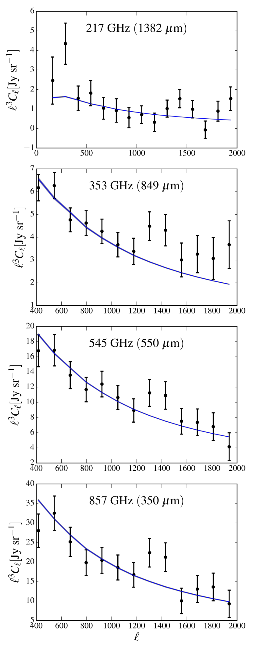
Figure 18: Correlation between CFIRB and CMB lensing potential (see Section 5.1) compared with our model prediction.

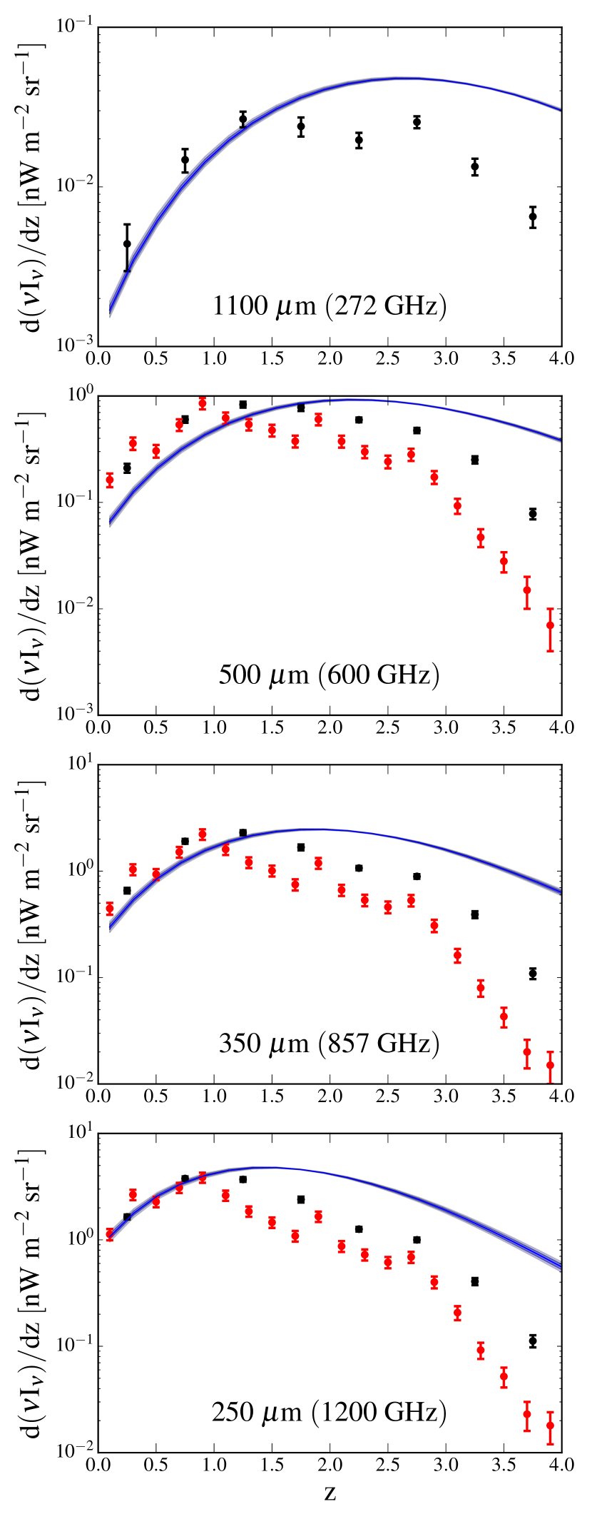
Figure 19: Redshift distribution of CFIRB (see Section 5.4) compared with our model prediction.

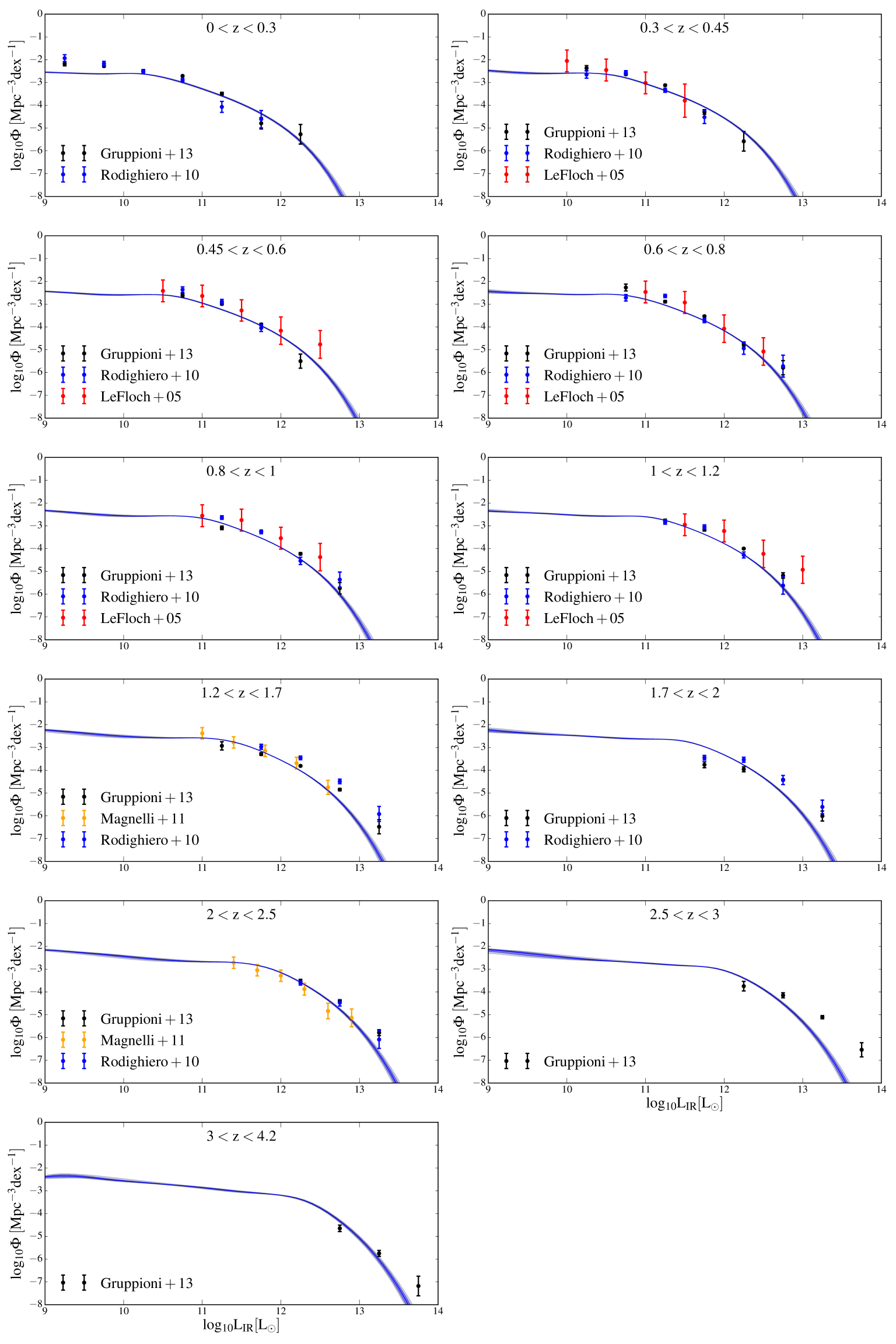
Figure 20: Bolometric infrared luminosity functions (see Section 5.2) compared with our model prediction.

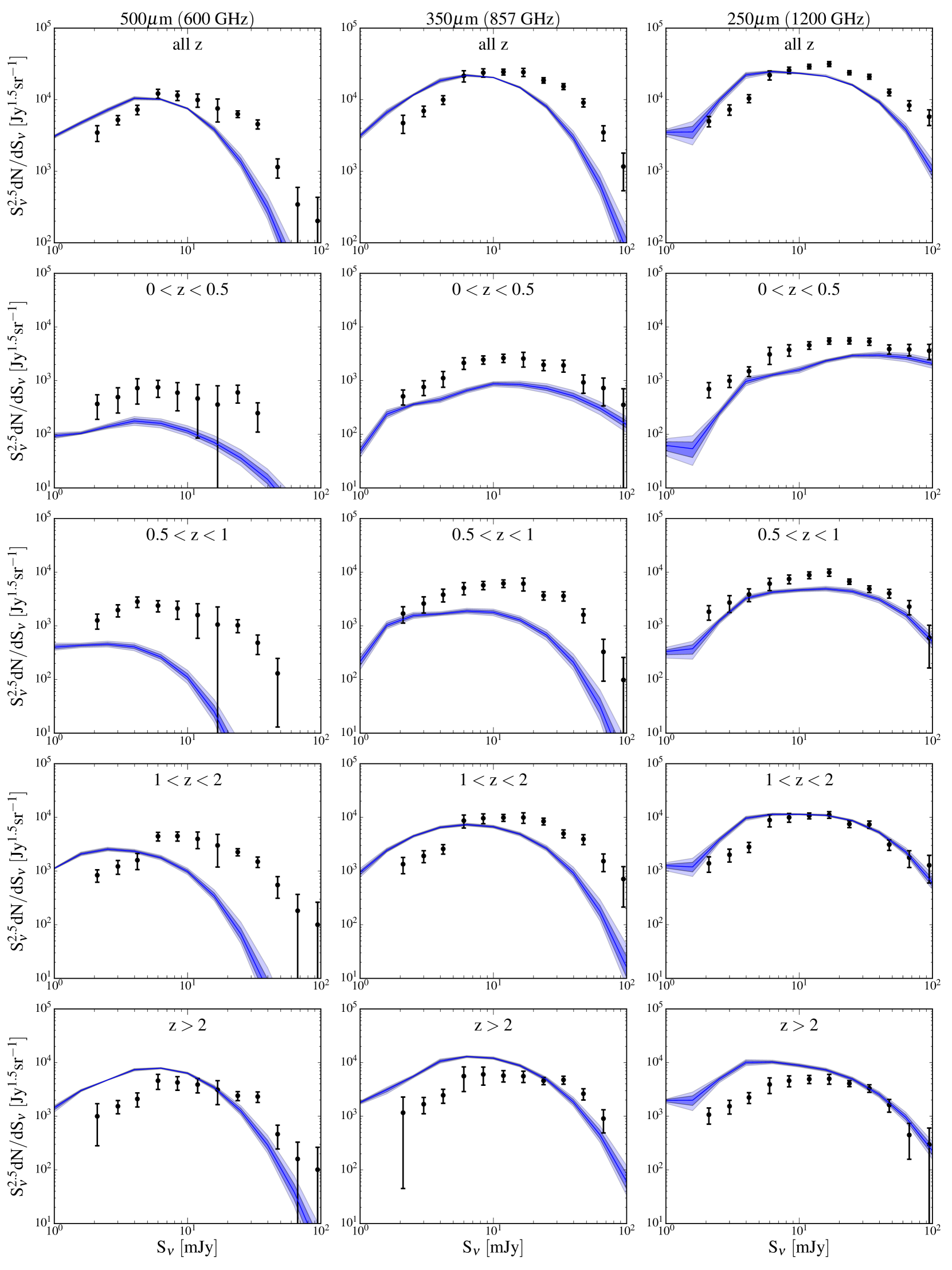
Figure 21: Number counts data from Béthermin et al. (2012, see Section 5.3) compared with our model prediction.

References

- Addison et al. (2013) Addison G. E., Dunkley J., Bond J. R., 2013, MNRAS, 436, 1896
- Alexander & Hickox (2012) Alexander D. M., Hickox R. C., 2012, New Astronomy Reviews, 56, 93
- Alexander et al. (2005) Alexander D. M., Bauer F. E., Chapman S. C., Smail I., Blain A. W., Brandt W. N., Ivison R. J., 2005, ApJ, 632, 736
- Amblard et al. (2011) Amblard A., et al., 2011, Nature, 470, 510
- Behroozi et al. (2013) Behroozi P. S., Wechsler R. H., Conroy C., 2013, ApJ, 770, 57
- Benson (2010) Benson A. J., 2010, Phys. Rep., 495, 33
- Benson et al. (2003) Benson A. J., Bower R. G., Frenk C. S., Lacey C. G., Baugh C. M., Cole S., 2003, ApJ, 599, 38
- Bernhard et al. (2014) Bernhard E., Béthermin M., Sargent M., Buat V., Mullaney J. R., Pannella M., Heinis S., Daddi E., 2014, MNRAS, 442, 509
- Berta et al. (2011) Berta S., et al., 2011, A&A, 532, A49
- Béthermin et al. (2012) Béthermin M., et al., 2012, A&A, 542, A58
- Béthermin et al. (2013) Béthermin M., Wang L., Doré O., Lagache G., Sargent M., Daddi E., Cousin M., Aussel H., 2013, A&A, 557, A66
- Béthermin et al. (2017) Béthermin M., et al., 2017, A&A, 607, A89
- Bond et al. (1986) Bond J. R., Carr B. J., Hogan C. J., 1986, ApJ, 306, 428
- Boselli et al. (2012) Boselli A., Ciesla L., Cortese L., et al., 2012, A&A, 540, A54
- Bouché et al. (2010) Bouché N., et al., 2010, ApJ, 718, 1001
- Chapman et al. (2005) Chapman S. C., Blain A. W., Smail I., Ivison R. J., 2005, ApJ, 622, 772
- Chen et al. (2010) Chen Y.-M., Tremonti C. A., Heckman T. M., Kauffmann G., Weiner B. J., Brinchmann J., Wang J., 2010, AJ, 140, 445
- Clements et al. (2014) Clements D. L., Braglia F. G., Hyde A. K., et al., 2014, MNRAS, 439, 1193
- Cooray & Sheth (2002) Cooray A., Sheth R., 2002, Phys. Rep., 372, 1
- Croton et al. (2006) Croton D. J., et al., 2006, MNRAS, 365, 11
- De Bernardis & Cooray (2012) De Bernardis F., Cooray A., 2012, ApJ, 760, 14
- De Zotti et al. (2015) De Zotti G., et al., 2015, J. Cosmol. Astropart. Phys., 6, 018
- Dekel & Mandelker (2014) Dekel A., Mandelker N., 2014, MNRAS, 444, 2071
- Dekel et al. (2013) Dekel A., Zolotov A., Tweed D., Cacciato M., Ceverino D., Primack J. R., 2013, MNRAS, 435, 999
- Draine & Lee (1984) Draine B. T., Lee H. M., 1984, ApJ, 285, 89
- Driver et al. (2007) Driver S. P., Popescu C. C., Tuffs R. J., Liske J., Graham A. W., Allen P. D., de Propris R., 2007, MNRAS, 379, 1022
- Dunne et al. (2011) Dunne L., Gomez H. L., da Cunha E., et al., 2011, MNRAS, 417, 1510
- Dutton & van den Bosch (2009) Dutton A. A., van den Bosch F. C., 2009, MNRAS, 396, 141
- Elbaz et al. (2002) Elbaz D., Cesarsky C. J., Chanial P., Aussel H., Franceschini A., Fadda D., Chary R. R., 2002, A&A, 384, 848
- Erb (2015) Erb D. K., 2015, Nature, 523, 169
- Fakhouri et al. (2010) Fakhouri O., Ma C.-P., Boylan-Kolchin M., 2010, MNRAS, 406, 2267
- Feldmann (2015) Feldmann R., 2015, MNRAS, 449, 3274
- Fixsen et al. (1998) Fixsen D. J., Dwek E., Mather J. C., Bennett C. L., Shafer R. A., 1998, ApJ, 508, 123
- Foreman-Mackey (2016) Foreman-Mackey D., 2016, The Journal of Open Source Software, 24
- Foreman-Mackey et al. (2013) Foreman-Mackey D., Hogg D. W., Lang D., Goodman J., 2013, PASP, 125, 306
- Fukugita & Peebles (2004) Fukugita M., Peebles P. J. E., 2004, ApJ, 616, 643
- Fumagalli et al. (2014) Fumagalli M., et al., 2014, ApJ, 796, 35
- Gelman & Rubin (1992) Gelman A., Rubin D. B., 1992, Statistical Science, 7, 457
- Gispert et al. (2000) Gispert R., Lagache G., Puget J. L., 2000, A&A, 360, 1
- Grossan & Smoot (2007) Grossan B., Smoot G. F., 2007, A&A, 474, 731
- Groves et al. (2012) Groves B., et al., 2012, MNRAS, 426, 892
- Gruppioni et al. (2013) Gruppioni C., et al., 2013, MNRAS, 432, 23
- Guo et al. (2011) Guo Q., et al., 2011, MNRAS, 413, 101
- Hajian et al. (2012) Hajian A., et al., 2012, ApJ, 744, 40
- Hall et al. (2010) Hall N. R., et al., 2010, ApJ, 718, 632
- Hauser & Dwek (2001) Hauser M. G., Dwek E., 2001, ARA&A, 39, 249
- Hauser et al. (1998) Hauser M. G., et al., 1998, ApJ, 508, 25
- Hayward et al. (2011) Hayward C. C., Kereš D., Jonsson P., Narayanan D., Cox T. J., Hernquist L., 2011, ApJ, 743, 159
- Hayward et al. (2012) Hayward C. C., Jonsson P., Kereš D., Magnelli B., Hernquist L., Cox T. J., 2012, MNRAS, 424, 951
- Hayward et al. (2014) Hayward C. C., et al., 2014, MNRAS, 445, 1598
- Heinis et al. (2014) Heinis S., et al., 2014, MNRAS, 437, 1268
- Hopkins et al. (2012) Hopkins P. F., Quataert E., Murray N., 2012, MNRAS, 421, 3522
- Hwang et al. (2010) Hwang H. S., Elbaz D., Magdis G., et al., 2010, MNRAS, 409, 75
- Jonsson et al. (2006) Jonsson P., Cox T. J., Primack J. R., Somerville R. S., 2006, ApJ, 637, 255
- Kennicutt (1998) Kennicutt Jr. R. C., 1998, ApJ, 498, 541
- Kistler et al. (2009) Kistler M. D., Yüksel H., Beacom J. F., Hopkins A. M., Wyithe J. S. B., 2009, ApJ, 705, L104
- Kogut et al. (2011) Kogut A., et al., 2011, J. Cosmol. Astropart. Phys., 7, 25
- Krumholz & Dekel (2012) Krumholz M. R., Dekel A., 2012, ApJ, 753, 16
- Lagache & Puget (2000) Lagache G., Puget J. L., 2000, A&A, 355, 17
- Lagache et al. (2007) Lagache G., Bavouzet N., Fernandez-Conde N., Ponthieu N., Rodet T., Dole H., Miville-Deschênes M.-A., Puget J.-L., 2007, ApJ, 665, L89
- Le Floc’h et al. (2005) Le Floc’h E., Papovich C., Dole H., et al., 2005, ApJ, 632, 169
- Le Floc’h et al. (2007) Le Floc’h E., Willmer C. N. A., Noeske K., et al., 2007, ApJ, 660, L65
- Lewis et al. (2000) Lewis A., Challinor A., Lasenby A., 2000, ApJ, 538, 473
- Lilly et al. (2013) Lilly S. J., Carollo C. M., Pipino A., Renzini A., Peng Y., 2013, ApJ, 772, 119
- Lutz et al. (2005) Lutz D., Valiante E., Sturm E., et al., 2005, ApJ, 625, L83
- Lutz et al. (2010) Lutz D., Mainieri V., Rafferty D., et al., 2010, ApJ, 712, 1287
- Madau & Dickinson (2014) Madau P., Dickinson M., 2014, ARA&A, 52, 415
- Magnelli et al. (2011) Magnelli B., Elbaz D., Chary R. R., Dickinson M., Le Borgne D., Frayer D. T., Willmer C. N. A., 2011, A&A, 528, A35
- Magnelli et al. (2012) Magnelli B., Lutz D., Santini P., et al., 2012, A&A, 539, A155
- Mak et al. (2017) Mak D. S. Y., Challinor A., Efstathiou G., Lagache G., 2017, MNRAS, 466, 286
- Martin et al. (2012) Martin C. L., Shapley A. E., Coil A. L., Kornei K. A., Bundy K., Weiner B. J., Noeske K. G., Schiminovich D., 2012, ApJ, 760, 127
- Matsuhara et al. (2000) Matsuhara H., Kawara K., Sato Y., et al., 2000, A&A, 361, 407
- Ménard & Fukugita (2012) Ménard B., Fukugita M., 2012, ApJ, 754, 116
- Mitchell-Wynne et al. (2015) Mitchell-Wynne K., et al., 2015, Nature Communications, 6, 7945
- Murray et al. (2005) Murray N., Quataert E., Thompson T. A., 2005, ApJ, 618, 569
- Narayanan et al. (2015) Narayanan D., et al., 2015, Nature, 525, 496
- Navarro et al. (1997) Navarro J. F., Frenk C. S., White S. D. M., 1997, ApJ, 490, 493
- Partridge & Peebles (1967) Partridge R. B., Peebles P. J. E., 1967, ApJ, 148, 377