1 Introduction

Recently, a significant progress has been made in the computation of the structure constants of planar $\mathcal{N}=4$ SYM by integrability techniques. The use of integrability to tackle this problem was initiated mostly in the papers [1, 2, 3] and culminated in a non-perturbative proposal formulated in [4]. This conjectured all-loop solution is grounded on a very stringy picture. The three-point functions are represented by a pair of pants corresponding to the well known idea of the splitting of a string into two other strings. Upon cutting open this pair of pants one is left with two hexagons patches with their edges identified. The hexagons are then regarded as a sort of fundamental objects that inherit information about the initial and final states. In particular, in the integrability language the external states are characterized by a set of parameters named Bethe rapidities and as a consequence the hexagons form-factors are functions of these rapidities. Eventually in [4] it was possible to bootstrap completely the so-called hexagon form-factors mostly by symmetry considerations. Once they are known, the structure constants can be obtained by gluing a pair of these hexagons and the final outcome is expressed in terms of sums over partitions of the Bethe rapidities of each operator. Several checks of the hexagon program predictions against the perturbative data were already made in the original paper [4]. Additional checks were made both at strong and weak coupling in [5, 6, 7, 8, 9, 10] providing very strong support for the correctness of the hexagon solution to the structure constants problem.

In this paper, we concentrate on operators sitting in the closed $\mathfrak{su}(1|1)$ sector which is the smallest sector containing fermionic excitations and consider their asymptotic three-point functions. This means that we take all the lengths involved to be large. In the hexagon language, the finite size corrections are controlled by the mirror particles and thus we can safely neglect them in this regime. One of the goals of this work is to check the predictions of the hexagon program for fermionic correlators against the perturbative data. We have found perfect agreement in all cases considered provided we include some ad hoc partition dependent additional signs in the hexagon program. This rule differs from the original proposal of [4], which already included some put-on signs to cohere with data, and we do not have a convincing geometric explanation for their origin.

In the section 2, we express the $\mathfrak{su}(1|1)$ primary operators in terms of some polarization vectors and directly compute the most general tree-level structure constant involving three of these operators. We prove that the result admits a determinant expression depending on the Bethe rapidities parametrizing the excitations of the three operators. In general, the result of a three-point function is a sum of many inequivalent tensor structures [11, 12, 13]. However in all cases considered in this work there is only one tensor structure (and consequentially one structure constant) and therefore it will be omitted everywhere. We refer the reader to [14] for details.

In the section 3, we apply the hexagon program for the $\mathfrak{su}(1|1)$ sector. Firstly, the case of one BPS and two non-BPS operators is considered. We prove by deriving recursion relations that the relevant hexagon form-factors for computing the structure constants in those cases can be explicitly evaluated and have a completely factorized form at all loops. Interestingly, the matrix part of these hexagon form-factors can be viewed as a partition function of a certain six-vertex model at any loop order. This fact is only true for operators in the $\mathfrak{su}(1|1)$ sector. A similar setup but with operators in the $\mathfrak{su}(2)$ sector was considered in the Appendix K of [4] and the hexagon form-factors are domain wall partition functions of a six-vertex model only at tree-level. This is the expected result because at tree-level the three-point function reduces to an off-shell scalar product [15, 16, 17]. In addition, we take the strong coupling limit of our results for the structure constants in the so-called BMN regime. Surprisingly, we show that the leading contribution to the structure constants can be written as a determinant for any number of excitations.

The case of three non-BPS operators is also studied in the section 3. In [14], the one-loop structure constants for specific three $\mathfrak{su}(1|1)$ operators were computed both by finding the two-loop Bethe eigenstates and by evaluating all the relevant Feynman diagrams. We have checked numerically that the hexagon program reproduces the results of [14]. The final answer for the structure constants in the hexagon program is given as a sum over partitions of three sets of Bethe rapidities (one for each operator) of the product of two hexagons form-factors. It is clearly a quite demanding task to explicitly compute them for a large number of excitations. It is very likely though that this solution can be further simplified at least for some cases. Three instances where such simplifications were attained are the determinant expressions of section 2 and subsection 3.2.2, the final expression for the structure constants of three $\mathfrak{su}(1|1)$ operators of [14] and the results of [10] in the semiclassical limit.

2 General tree-level structure constants in $\mathfrak{su}(1|1)$

In this section, we consider the most general configuration of operators in the $\mathfrak{su}(1|1)$ sector of $\mathcal{N}=4$ SYM. There are different embeddings of $\mathfrak{su}(1|1)$ in the full superconformal group and they can be conveniently parametrized through some polarization vectors. This has a resemblance with the studies made in the $\mathfrak{su}(2)$ sector presented in [18].

The $R$-charge index contractions in the three-point functions considered here are nicely accounted by the scalar products of the polarization vectors. It then remains to compute the dynamical part which is the most interesting one. At tree-level, we make full use of the fact that these operators are described by free fermions and we are able to derive a determinant expression for the structure constants.

2.1 Polarization vectors for $\mathfrak{su}(1|1)$

In order to parametrize the external operators in the three-point function, let us start by introducing a pair of polarization vectors $Z_{a}$ and $W_{a}$, where $a=1,\ldots,4$ are $\mathfrak{su}(4)$ indices, satisfying the following normalization and orthogonality conditions

$$\bar{Z}^{a}Z_{a}=1\,,\quad\bar{W}^{a}W_{a}=1\,,\quad\bar{Z}^{a}W_{a}=0\,,\quad\bar{W}^{a}Z_{a}=0\,,$$ (2.1)

with the bar standing for the usual complex conjugation $\bar{Z}^{a}\equiv(Z_{a})^{*}$.

A state in the $\mathfrak{su}(1|1)$ sector is built out of a scalar field $\mathnormal{\Phi}$ and a fermionic field $\mathnormal{\Psi}$ that we define in terms of the above polarization vectors by

$$\mathnormal{\Phi}=Z_{a}W_{b}\,\phi^{ab}\,,\quad\mathnormal{\Psi}=W_{a}\,\psi^{a}-Z_{c}\,\psi^{c}\,,$$ (2.2)

where $\phi^{ab}$ and $\psi^{c}$ are the scalar and fermion fields of $\mathcal{N}=4$ SYM and we have omitted the Lorentz index $\alpha$ of the fermions, as we fix it once and for all to take the value $\alpha=1$. We now want to show that the fields $\mathnormal{\Phi}$ and $\mathnormal{\Psi}$ form a representation of the tree-level algebra. For that let us define a supercharge $\mathcal{Q}$ as follows

$$\mathcal{Q}\equiv\bar{Z}^{a}Q_{a}^{1}+\bar{W}^{a}Q_{a}^{1}\,,$$ (2.3)

where $Q_{a}^{\alpha}$ is the standard bare supercharge that generates the usual supersymmetry transformations on the fields

$$[Q_{a}^{\alpha}\,,\phi^{bc}]=\delta^{b}_{a}\psi^{c\alpha}-\delta^{c}_{a}\psi^{b\alpha}\,,\quad\quad[Q_{a}^{\alpha},\psi^{b}_{\beta}]=\delta^{b}_{a}F^{\alpha}_{\beta}\,,$$ (2.4)

where $F^{\alpha}_{\beta}$ is the self-dual field-strength. We then observe that the relations $\mathcal{Q}\,\mathnormal{\Phi}=\mathnormal{\Psi}$ and $\mathcal{Q}\,\mathnormal{\Psi}=0$ hold which imply a $\mathfrak{su}(1|1)$ representation.

A general $\mathfrak{su}(1|1)$ primary operator can then be defined by specifying a pair of vectors $(Z_{a},W_{a})$. For example, an operator $\mathcal{O}$ with $N$ excitations and length $L$ is defined by

$$\mathcal{O}(Z,W)=\sum_{1\leq n_{1}<\ldots<n_{N}\leq L}\psi_{n_{1},n_{2},\ldots,n_{N}}\,\text{Tr}\,(\mathnormal{\Phi}\dots\underset{n_{1}}{\mathnormal{\Psi}}\dots\underset{n_{2}}{\mathnormal{\Psi}}\dots\mathnormal{\Phi}),$$ (2.5)

where the dependence in the polarization vectors is hidden in $\mathnormal{\Phi}$ and $\mathnormal{\Psi}$ and $\psi$ is a wave-function (we are omitting the $\mathfrak{su}(4)$ index $a$ to simplify the notation).

The contraction of the $R$-charge indices between two given scalar fields parameterized by $(Z^{(1)},W^{(1)})$ and $(Z^{(2)},W^{(2)})$ respectively, gives the following contribution

$$\langle\mathnormal{\Phi}^{(1)}\mathnormal{\Phi}^{(2)}\rangle =Z^{(1)}_{a}W^{(1)}_{b}Z^{(2)}_{c}W^{(2)}_{d}\,\langle\phi^{ab}\phi^{cd}\rangle$$ (2.6)

$$=\det[\{Z^{(1)},W^{(1)},Z^{(2)},W^{(2)}\}]$$

$$\equiv\langle 12\rangle\,.$$

Analogously, we have that the contraction of a scalar $\mathnormal{\Phi}^{(1)}$ and a conjugate scalar $\bar{\mathnormal{\Phi}}^{(2)}$ is given by

$$\langle\mathnormal{\Phi}^{(1)}\bar{\mathnormal{\Phi}}^{(2)}\rangle =Z^{(1)}_{a}W^{(1)}_{b}\bar{Z}^{(2)\,c}\,\bar{W}^{(2)\,d}\,\langle\phi^{ab}\phi_{cd}\rangle$$ (2.7)

$$=Z^{(1)}_{a}W^{(1)}_{b}\left(\bar{Z}^{(2)\,a}\,\bar{W}^{(2)\,b}-\bar{Z}^{(2)\,b}\,\bar{W}^{(2)\,a}\right)$$

$$\equiv\langle 1\bar{2}\rangle\,.$$

Finally for the fermions, one has

$$\langle\mathnormal{\Psi}^{(1)}\bar{\mathnormal{\Psi}}^{(2)}\rangle =(Z^{(1)}_{a}-W^{(1)}_{a})(\bar{Z}^{(2)\,b}-\bar{W}^{(2)\,b})\,\langle\psi^{a}\bar{\psi}_{b}\rangle$$ (2.8)

$$=(Z^{(1)}_{a}-W^{(1)}_{a})(\bar{Z}^{(2)\,a}-\bar{W}^{(2)\,a})$$

$$\equiv[1\bar{2}]\,.$$

The setup we will be considering in this section is formed by three operators of the type (2.5), each one characterized by a pair of polarization vectors $(Z^{(i)},W^{(i)})$ for $i=1,2,3.$ Moreover, in order to have a non-zero structure constant, we conventionally take the operator $\mathcal{O}_{2}$ to have the antichiral fermions, that is

$$\mathcal{O}_{2}(\bar{Z}^{(2)},\bar{W}^{(2)})=\sum_{1\leq n_{1}<\ldots<n_{N_{2}}\leq L_{2}}\psi^{(2)}_{n_{1},n_{2},\ldots,n_{N_{2}}}\,\text{Tr}\,(\bar{\mathnormal{\Phi}}^{(2)}\dots\underset{n_{1}}{\bar{\mathnormal{\Psi}}}^{(2)}\dots\underset{n_{2}}{\bar{\mathnormal{\Psi}}}^{(2)}\dots\bar{\mathnormal{\Phi}}^{(2)})\,.$$ (2.9)

We will now make use of this parametrization of the operators to compute the tree-level structure constants.

2.2 Tree-level three-point functions as a determinant

At tree-level, the wave-function $\psi^{(i)}$ associated to the operator $\mathcal{O}_{i}$ is given by the standard Bethe wave-function for a free fermion system that follows from the requirement that it diagonalizes the one-loop $\mathfrak{su}(1|1)$ Hamiltonian (more details can be found in [14]). It is given by

$$\psi^{(i)}_{n_{1},n_{2},\ldots,n_{N_{i}}}=\sum_{P}\,(-1)^{P}\,{\rm{exp}}(ip^{(i)}_{\sigma_{P}(1)}n_{1}+ip^{(i)}_{\sigma_{P}(2)}n_{2}+\ldots+ip^{(i)}_{\sigma_{P}(N_{i})}n_{N_{i}})\,,$$ (2.10)

where $P$ indicates sum over all possible permutations $\sigma_{P}$ of the elements $\{1,...,N_{i}\}$, and $(-1)^{P}$ is the sign of the permutation. In addition, the momenta satisfy the Bethe equations

$$e^{ip^{(i)}_{j}L_{i}}=1\,.$$ (2.11)

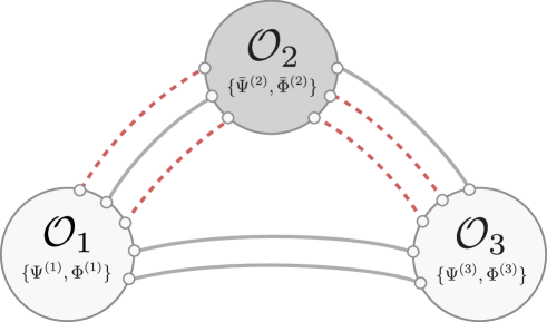
Figure 1: This figure illustrates the Wick contractions for the computation of the tree-level three-point function in the most general $\mathfrak{su}(1|1)$ setup. The dashed (solid) lines correspond to fermions (scalars) propagators. It is clear from the figure that one should multiply the three wave-functions corresponding to each of the operators and perform a sum over the positions of the fermionic excitations. In our conventions, all the operators are oriented clockwise.

The tree-level structure constant is simply given by the product of the three wave-functions with the positions of the excitations of each operator summed over, see figure 1 for clarity. Concretely, we have the following nested sums to evaluate

$$C_{123}=\mathcal{R}\sum_{\begin{subarray}{c}1\leq n_{1}<\ldots<n_{N_{1}}\leq l_{12}\\ 1\leq m_{1}<\ldots<m_{N_{3}}\leq l_{23}\end{subarray}}\psi^{(1)}_{L_{1}-n_{N_{1}}+1,\ldots,L_{1}-n_{1}+1}\psi^{(2)}_{n_{1},\ldots,n_{N_{1}},l_{12}+m_{1},\ldots,l_{12}+m_{N_{3}}}\psi^{(3)}_{l_{23}-m_{N_{3}}+1,\ldots,l_{23}-m_{1}+1}\,,$$ (2.12)

where $\mathcal{R}$ includes the contribution from the $R$-charge contractions and the normalization factor and reads

$$\mathcal{R}=\sqrt{\frac{L_{1}L_{2}L_{3}}{{\mathcal{N}}^{(1)}{\mathcal{N}}^{(2)}{\mathcal{N}}^{(3)}}}\,\,\,\langle 13\rangle^{l_{13}}[3\bar{2}]^{N_{3}}\langle 3\bar{2}\rangle^{l_{23}-N_{3}}[1\bar{2}]^{N_{1}}\langle 1\bar{2}\rangle^{l_{12}-N_{1}}\,,$$ (2.13)

where $\mathcal{N}^{(i)}$ is the norm of the wave-function $\psi^{(i)}$ and $l_{ij}$ is the number of contractions between operators $i$ and $j$.

Given that the wave-functions in (2.10) are completely antisymmetric in all their arguments, we can extend the sums in (2.12) at the price of introducing a trivial overall combinatorial factor. Plugging their explicit expressions, we are left with

$$\frac{C_{123}}{\mathcal{R}}=\sum_{\{n_{i}\},\{m_{i}\}}\sum_{P,\,Q,\,S}\frac{(-1)^{P+Q+S}}{N_{1}!N_{3}!}\,\times\,\hskip 184.9429pt$$ (2.14)

$$\prod_{a=1}^{N_{1}}\prod_{b=1}^{N_{3}}e^{ip^{(1)}_{P(N_{1}-a+1)}(1-n_{a})}e^{ip^{(2)}_{S(a)}n_{a}}e^{ip^{(2)}_{S(N_{1}+b)}(l_{12}+m_{b})}e^{ip^{(3)}_{Q(N_{3}-b+1)}(l_{23}-m_{b}+1)}\,,$$

where we have simplified the wave-function of the operator $\mathcal{O}_{1}$ by using the Bethe equations. Note that the sums over $n_{i}$ and $m_{i}$ are not ordered anymore and run through the full range $1\leq n_{i}\leq l_{12}$ and $1\leq m_{i}\leq l_{23}$. It is now simple to perform the sums over $n_{i}$ and $m_{i}$ as they are geometric series. This results in

$$\frac{C_{123}}{\mathcal{R}}=\sum_{P,\,Q,\,S}\frac{(-1)^{P+Q+S}}{N_{1}!N_{3}!}\,\prod_{a=1}^{N_{1}}\prod_{b=1}^{N_{3}}\,\frac{1-e^{i\left(p^{(2)}_{S(a)}-p^{(1)}_{P(N_{1}+1-a)}\right)l_{12}}}{e^{-ip^{(2)}_{S(a)}}-e^{-ip^{(1)}_{P(N_{1}+1-a)}}}\times\frac{e^{-i\left(p^{(2)}_{S(N_{1}+b)}-p^{(3)}_{Q(N_{3}+1-b)}\right)l_{23}}-1}{e^{-ip^{(2)}_{S(N_{1}+b)}}-e^{-ip^{(3)}_{Q(N_{3}+1-b)}}}.$$ (2.15)

It is not hard to recognize this expression as being, apart for some signs, the definition of the determinant of a $N_{2}$ by $N_{2}$ matrix formed by two blocks namely,

$$C_{123}=\mathcal{R}\,(-1)^{\frac{N_{1}(N_{1}-1)}{2}}\,(-1)^{\frac{N_{3}(N_{3}-1)}{2}}\,\det_{1\leq j,k\leq N_{2}}\left[C^{(1)}_{jk}\oplus C^{(3)}_{jk}\right]$$ (2.16)

with the blocks being

$$C^{(1)}_{jk}=\frac{1-e^{i\left(p^{(2)}_{j}-p^{(1)}_{k}\right)l_{12}}}{e^{-ip^{(2)}_{j}}-e^{-ip^{(1)}_{k}}}\,,\,\,\,\,\,j=1,\dots,N_{2},\,\,k=1,\dots,N_{1}\,,$$ (2.17)

$$C^{(3)}_{jk}=\frac{e^{-i\left(p^{(2)}_{j}-p^{(3)}_{k}\right)l_{23}}-1}{e^{-ip^{(2)}_{j}}-e^{-ip^{(3)}_{k}}}\,,\,\,\,\,\,j=1,\dots,N_{2},\,\,k=1,\dots,N_{3}\,.$$

This is the main result of this section. In what follows we will consider a few limits of this expression.

Extremal limit

In the extremal limit $L_{2}=L_{1}+L_{3}$ which implies that $l_{23}=L_{3}$ and $l_{12}=L_{1}$. Inserting these conditions on the previous formula, it gets simplified once we use the Bethe equations and both blocks get a similar form

$$C_{jk}^{(1)}=\frac{1-e^{ip^{(2)}_{j}L_{1}}}{e^{-ip^{(2)}_{j}}-e^{-ip^{(1)}_{k}}}\,,\quad\quad\quad C_{jk}^{(3)}=-\frac{1-e^{ip^{(2)}_{j}L_{1}}}{e^{-ip^{(2)}_{j}}-e^{-ip^{(3)}_{k}}}\,.$$ (2.18)

It immediately follows that this is a Cauchy matrix and one can use the Cauchy determinant formula to obtain

$$C_{123}=\mathcal{R}\,(-1)^{N_{3}}\,\prod\limits_{i=1}^{N_{2}}{\left(1-e^{ip^{(2)}_{i}L_{1}}\right)}\frac{\prod\limits_{k=1}^{3}\prod\limits_{i>j}^{N_{k}}\mathfrak{f}^{(kk)}_{ij}\prod\limits_{i=1}^{N_{1}}\prod\limits_{j=1}^{N_{3}}\mathfrak{f}^{(13)}_{ij}}{\prod\limits_{i=1}^{N_{2}}\prod\limits_{j=1}^{N_{1}}\mathfrak{f}^{(21)}_{ij}\prod\limits_{i=1}^{N_{2}}\prod\limits_{j=1}^{N_{3}}\mathfrak{f}^{(23)}_{ij}}\,,$$ (2.19)

where we have defined

$$\mathfrak{f}_{ij}^{(km)}\equiv e^{-ip^{(k)}_{i}}-e^{-ip^{(m)}_{j}}\,.$$ (2.20)

In addition to this, the extremal case gets modified by the contribution coming from the one-loop mixing of the single-trace $\mathcal{O}_{2}$ with the double-trace operators. The calculation of this extra piece is outside the scope of the present paper and we leave it for future work.

Reduction to the formula of [14]

Another limit where the determinant (LABEL:determinant) gets factorized is the configuration considered in [14]. In that setup, one sets $l_{23}=N_{3}$ which leads to

$$|C_{123}|=\mathcal{R}\left|\,\prod\limits_{i=1}^{N_{1}}{\left(1-e^{ip^{(1)}_{i}L_{2}}\right)}\frac{\prod\limits_{k=1}^{3}\prod\limits_{j<i}^{N_{k}}\mathfrak{f}^{(kk)}_{ji}}{\prod\limits_{i=1}^{N_{2}}\prod\limits_{j=1}^{N_{1}}\mathfrak{f}^{(21)}_{ij}}\,\right|\,.$$ (2.21)

where $\mathfrak{f}_{ij}^{(km)}$ was defined in (2.20).

3 Hexagon program for fermionic correlators

In this section, we will compute three-point functions of operators containing fermionic excitations using the hexagon program of [4]. This method generates all-loop predictions for the structure constants which as we will see match the results of the previous section when expanded at leading order. Firstly, we will briefly review the definition of the hexagon form-factor. We then show that the relevant hexagon for the three-point function of one BPS and two non-BPS operators in the $\mathfrak{su}(1|1)$ sector has the interpretation of a domain wall partition function of a certain six-vertex model. We further prove that it has a completely factorized form to all loops. We perform checks with the available data for fermionic correlators and point out the need of some additional relative signs when the two hexagon form-factors are combined together to form the three-point function in order to get a match.

3.1 Fermionic hexagons

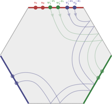
Figure 2: When computing three-point functions using the hexagon program, we only need to consider the hexagon form-factor with excitations in a single edge, say the red edge in the figure. When more than one operator is excited, some of the excitations on the red edge will be mirror transformed. In the figure we identify the rapidities of the corresponding mirror transformed excitations by the upper symbol $\gamma$. This corresponds to having moved them from the red edge to other edges of the hexagon. In particular an even number of such mirror transformations move them to other physical edges, represented in green and blue in the figure. The particular edge where they end up depends on the sign and number of mirror transformations applied to them. The conventions we use here are illustrated in the figure.

The fundamental excitations of an operator in the hexagon program transform in the bifundamental representation of a centrally extended $\mathfrak{su}(2|2)\times\mathfrak{su}(2|2)$ algebra. They are labeled by two indices $(A\,,\dot{A})$. In our conventions, these indices take the values 1 to 4 with $a=1,2$ being bosonic indices and $\alpha=3,4$ fermionic ones. Throughout this section we will be considering fermionic excitations which carry both one bosonic and one fermionic index.

The hexagon form-factor in the string frame with $N$ excitations with rapidities $u_{i}$ in one physical edge (see figure 2) of the hexagon is given by [4]

$$h^{A_{1}\dot{B}_{1},\ldots,A_{N}\dot{B}_{N}}_{\rm{string}}(u_{1},\ldots,u_{N})=(-1)^{f}\prod_{i<j}h(u_{i},u_{j})\langle\chi_{N}^{\dot{B}_{N}}\ldots\chi_{1}^{\dot{B}_{1}}|\,\mathcal{S}\,|\chi_{1}^{{A}_{1}}\ldots\chi_{N}^{{A}_{N}}\rangle\,,$$ (3.1)

where $f=\sum_{i<j}{\rm{grad}}(\dot{B}_{i})\,{\rm{grad}}(A_{j})$ and grad means the grading of the corresponding index being equal to zero for bosonic indices and to one for fermionic indices. In the formula above, $\mathcal{S}$ is the $\mathfrak{su}(2|2)$ $S$-matrix in the string frame [19, 20, 21] with the overall multiplicative constant set to one and $(\chi^{A},\chi^{\dot{A}})$ are states in the fundamental of $\mathfrak{su}(2|2)\times\mathfrak{su}(2|2)$. In Appendix A we present the explicit form of the $S$-matrix used here. In order to evaluate the matrix part of the hexagon form-factor, one uses

$$\langle\chi_{N}^{\dot{B}_{N}}\ldots\chi_{1}^{\dot{B}_{1}}|\,\chi_{N}^{{A}_{N}}\ldots\chi_{1}^{{A}_{1}}\rangle=h^{A_{1}\dot{B}_{1}}\ldots\,h^{A_{N}\dot{B}_{N}}\,,$$ (3.2)

and the only nonvanishing components are

$$h^{1\dot{2}}=-h^{2\dot{1}}=1\,,\quad\quad h^{3\dot{4}}=-h^{4\dot{3}}=-i\,.$$ (3.3)

Finally, the function $h(u,v)$ is defined by

$$h(u,v)=\frac{x_{u}^{-}-x_{v}^{-}}{x_{u}^{-}-x_{v}^{+}}\frac{1-1/x_{u}^{-}x_{v}^{+}}{1-1/x_{u}^{+}x_{v}^{+}}\frac{1}{\sigma(u,v)}\,.$$ (3.4)

The variables $x$ are Zhukowsky variables satisfying $x_{u}+1/x_{u}=u/g$ with $g$ the coupling constant and $x_{u}^{\pm}=x\bigl{(}u\pm\frac{i}{2}\bigr{)}$. Moreover, $\sigma(u,v)$ is half the dressing phase of [22].

When computing a three-point function, we first transfer all the excitations of the three operators to one of the physical edges of the hexagon, see figure 2. This is done by performing successive mirror transformations on the excitations of certain operators. These mirror transformations correspond to an analytic continuation of the hexagon in the rapidities of the corresponding excitations. In Appendix A we present the transformation that the hexagon form-factor undergoes by this analytic continuation for the fermionic excitations. In addition to this, we will compare the predictions for the structure constants obtained using the hexagon program with the available weak coupling data. In order to perform these checks, we first do the computations using the string frame where the mirror transformations are implemented in a simple manner and then map the result to the spin-chain frame [23, 24]. The two frames are related by a phase depending on the momenta of the excitations and that is described in Appendix A.

3.2 All-loop factorization for 1 BPS and 2 non-BPS operators

In this subsection, we compute the structure constants of two non-BPS fermionic operators and one BPS operator using the hexagon program. We will further provide a closed expression for the hexagon form-factors in a completely factorized form.

The non-BPS operators are in the $\mathfrak{su}(1|1)$ sector and contain a single type of fermionic excitations. To fix the conventions, we choose a setup of three operators in which the operator $\mathcal{O}_{1}$ has the excitations $\mathnormal{\Psi}\equiv\chi^{3\dot{1}}$, the operator $\mathcal{O}_{2}$ has the excitations $\bar{\mathnormal{\Psi}}\equiv\chi^{2\dot{4}}$ and the operator $\mathcal{O}_{3}$ is BPS, see figure 3(a).

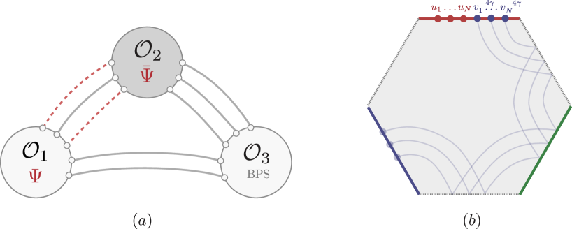
Figure 3: (a) We represent the tree-level configuration used in this section. The operator $\mathcal{O}_{1}$ ($\mathcal{O}_{2}$) contains $\mathnormal{\Psi}$ ($\bar{\mathnormal{\Psi}}$) excitations, $\mathcal{O}_{3}$ is BPS and it has no excitations. (b) The hexagon form-factor used in this section contains two types of excitations associated to the two non-BPS operators. A set of those excitations ($v_{i}$) are mirror transformed four times to the right (hence the minus sign in $-4\gamma$) and end up in the physical edge belonging to the operator $\mathcal{O}_{1}$. Alternatively we could have started with the excitations in the top edge with the positions of $u_{i}$ and $v_{i}$ reversed and performed two mirror transformations on the $v_{i}$ to the left. The first option is used in the main text as it makes the matrix part simpler.

In order to use the defining expression for the hexagon form-factors of (3.1), we need to move all the excitations to the upper edge of the hexagon. There are two possible ways of moving the excitation in the second physical edge to the upper edge. One can perform either one crossing transformation or minus two crossing transformations. We will choose the second possibility, see figure 3(b), for reasons of simplicity as will become clear below. Under this double crossing transformation, the fermionic excitations get their sign flipped according to the formula (A.16) of Appendix A. Taking these signs into account, we get that the central object of the three-point function for this setup is the following hexagon form-factor which we denote by $h_{\mathnormal{\Psi}_{1}\ldots\mathnormal{\Psi}_{N}|\bar{\mathnormal{\Psi}}_{1}\ldots\bar{\mathnormal{\Psi}}_{N}}$ and reads

$$h_{\mathnormal{\Psi}_{1}\ldots\mathnormal{\Psi}_{N}|\bar{\mathnormal{\Psi}}_{1}\ldots\bar{\mathnormal{\Psi}}_{N}}\equiv(-1)^{N}\prod_{i<j}h(u_{i},u_{j})\,h(v_{i}^{-4\gamma},v_{j}^{-4\gamma})\prod_{i,j}h(u_{i},v_{j}^{-4\gamma})\times[\texttt{matrix part}]\,,$$

$$[\texttt{matrix part}]=\langle\chi_{v^{-4\gamma}_{N}}^{\dot{4}}\dots\chi_{v^{-4\gamma}_{1}}^{\dot{4}}\chi_{u_{N}}^{\dot{1}}\dots\chi_{u_{1}}^{\dot{1}}|\,\mathcal{S}\,|\chi_{u_{1}}^{{3}}\ldots\chi_{u_{N}}^{{3}}\chi_{v_{1}^{-4\gamma}}^{{2}}\ldots\chi_{v_{N}^{-4\gamma}}^{{2}}\rangle\,.\hskip 31.29802pt$$ (3.5)

Recall that we evaluate this form-factor in the string frame normalization. When we will later compare with data, we will then map it to the spin-chain frame using the conversion factor in formula (A.18). As an illustration, let us first compute the simplest case namely $h_{\mathnormal{\Psi}|\bar{\mathnormal{\Psi}}}(u,v)$. We find

$$h_{\mathnormal{\Psi}|\bar{\mathnormal{\Psi}}}(u,v)=-h(u,v^{-4\gamma})\langle\chi_{v^{-4\gamma}}^{\dot{4}}\,\chi_{u}^{\dot{1}}|\,\mathcal{S}\,|\chi_{u}^{{3}}\,\chi_{v^{-4\gamma}}^{{2}}\rangle=-\frac{i}{h(v,u)}K_{uv^{-4\gamma}}\,,$$ (3.6)

where the $S$-matrix element $K$ is defined in the Appendix A. Moreover, we have used the following properties of the dressing phase to write $h(u,v^{-4\gamma})$ in terms of $h(v,u)$,

$$\sigma(u^{2\gamma},v)\sigma(u,v)=\frac{(1-1/x^{+}_{u}x^{+}_{v})}{(1-x^{-}_{u}/x^{-}_{v})}\frac{(1-x^{-}_{u}/x^{+}_{v})}{(1-1/x^{+}_{u}x^{-}_{v})}\,,\quad\quad\sigma(u,v)=\frac{1}{\sigma(v,u)}\,.$$ (3.7)

Let us consider now the general case when there are $N$ excitations $\mathnormal{\Psi}$ in the upper edge of the hexagon and $N$ excitations $\bar{\mathnormal{\Psi}}$ in the second physical edge of the hexagon. Using the formulae (A.13), we can immediately write the pre-factor in front of the matrix part in expression (3.5) after the inverse crossing transformation of the set of rapidities $\{v\}$, to get

$$h_{\mathnormal{\Psi}_{1}\ldots\mathnormal{\Psi}_{N}|\bar{\mathnormal{\Psi}}_{1}\ldots\bar{\mathnormal{\Psi}}_{N}}=(-1)^{N}\frac{\prod_{i<j}^{N}h(u_{i},u_{j})\prod_{i<j}^{N}h(v_{i},v_{j})}{\prod_{i,j}^{N}h(v_{i},u_{j})}\times[\texttt{matrix part}]\,.$$ (3.8)

One way of evaluating the matrix part above is to first scatter the excitations $\chi^{3}_{u_{i}}$ among themselves to put them in descending order. We can then scatter them with all the other $\chi^{2}_{{v_{i}}^{-4\gamma}}$. According to (A.1) this scattering will in general produce several terms where the indices can either be conserved or get swapped. Due to the one particle form-factor (3.3), the only non-zero $S$-matrix element occurs for the case where all the excitations $\chi^{3}_{u_{i}}$ swap their indices with $\chi^{2}_{{v_{i}}^{-4\gamma}}$. Finally, we scatter the resulting $\chi^{3}_{{v_{i}}^{-4\gamma}}$ to put them in descending order as well. The first and last step of this procedure where excitations of the same species scatter among themselves results in a trivial factor as the only $S$-matrix element playing a role is $D_{ij}=-1$.

Interestingly, the non-trivial part of this scattering process turns out to be equivalent up to a phase to the computation of a partition function that resembles a domain wall partition function of a certain six-vertex model as illustrated in figure 4(a) with the six nonzero vertices of figure 5.

The fact that we have a six-vertex model at any value of the coupling is remarkable and it is not true in general for other sectors. In the Appendix K of [4] for example, two non-BPS $\mathfrak{su}(2)$ operators were considered and they only have a six-vertex model at tree-level.

3.2.1 Factorization of the domain wall partition function

In this subsection, we will derive a closed expression for the partition function of Figure 4 valid at any value of the coupling constant. We will denote the partition function by ${\rm{\mathcal{P}}}_{N}\left(\{u_{1},\dots,u_{N}\},\{v_{1},\dots,v_{N}\}\right)$. From the properties of the $S$-matrix, we can immediately infer the following relations

1. ${\mathcal{P}}_{1}(\{u_{1}\},\{v_{1}\})=K_{u_{1}{{v_{1}}^{-4\gamma}}}\,,$

2. ${\mathcal{P}}_{N}(\{u\},\{v_{1},\ldots,v_{i},v_{i+1},\ldots,v_{N}\})=-A_{v_{i}v_{i+1}}\,{\mathcal{P}}_{N}(\{u\},\{v_{1},\ldots,v_{i+1},v_{i}\ldots,v_{N}\})\,,$

3. ${\mathcal{P}}_{N}(\{u_{1},\ldots,u_{i},u_{i+1},\ldots,u_{N}\},\{v\})=-A_{u_{i}u_{i+1}}\,{\mathcal{P}}_{N}(\{u_{1},\ldots,u_{i+1},u_{i},\ldots,u_{N}\},\{v\})\,.$

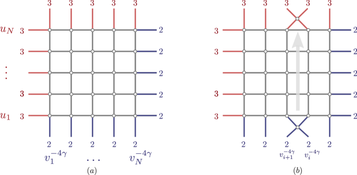
Figure 4: (a) The partition function appearing in the computation of the matrix part of the hexagon form-factor. The vertices at any value of the coupling are given in the figure 5. (b) The procedure to prove the relation II of $\mathcal{P}_{N}$ goes as follows. Inserting an additional vertex to the bottom of the partition function grid, it is possible to move it to the top using the Yang-Baxter equation with some rapidities crossed several times and remove it. The result is proportional to a grid with the two columns swapped. A similar procedure can be used to prove the relation III of $\mathcal{P}_{N}$ but this time the procedure involves two neighboring lines.

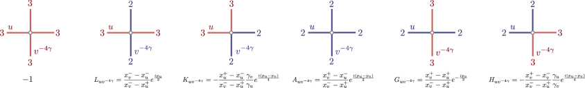
Figure 5: The nonzero six vertices used for computing the partition function and their respective weights which are equal to the components of the string frame $S$-matrix, see Appendix A.

The relation I simply follows from the fact that for $N=1$ the partition function reduces to the weight of the third vertex given in figure 5. The relations II and III follow from using repeatedly the Yang-Baxter equation and the vertices in figure 5 as illustrated in figure 4(b) (see also [25, 26]).

As a first step to compute this partition function, we can use the previous properties to immediately infer its dependence on the phases of momenta $e^{ip_{u_{k}}}$, $e^{ip_{v_{k}}}$ and $\gamma_{u_{k}}$, $\gamma_{v_{k}}$ where $\gamma_{u}=\sqrt{i(x^{-}_{u}-x^{+}_{u})}$. Consider the top horizontal line. It is not difficult to see that the only allowed vertices on that line are the first, third and fifth of figure 5. Moreover, the third vertex always appear only one time for each configuration on that line. Once it is used, then the whole line gets frozen. This vertex is the only among the allowed ones for the top line that depends on the momenta $p_{u_{N}}$ and $\gamma_{u_{N}}$. Therefore we can determine that the dependence of the whole partition function on these quantities comes from the weight of the third vertex.

A similar analysis can be performed on the first vertical line. The only allowed vertices are the first, second and the third ones and again the third vertex necessarily appears only one time in every configuration on that line. Analogously, given the weights of these three vertices, we deduce that the dependence of the partition function on $p_{v_{1}}$ and $\gamma_{v_{1}}$ comes solely from the weight of third vertex in the first vertical line.

Combining these observations with properties II and III, we can determine the dependence of the partition function on $p_{u_{k}},p_{v_{k}}$, $\gamma_{u_{k}}$ and $\gamma_{v_{k}}$ for every $k$ and it reads

$${\mathcal{P}}_{N}(\{u\},\{v\})=\prod_{k=1}^{N}\left[-\frac{\gamma_{v_{k}}}{\gamma_{u_{k}}}\,e^{-\frac{i}{2}p_{v_{k}}\left(k-1/2\right)}e^{-\frac{i}{2}p_{u_{k}}\left(k-1/2-N\right)}\right]\,{\mathcal{DW}}_{N}(\{u\},\{v\})\,,$$ (3.9)

where ${\mathcal{DW}}_{N}(\{u\},\{v\})$ is a domain wall partition function with the same boundary conditions of figure 4, but with the six vertices of figure 6 (it is possible this time to drop the $-4\gamma$ from $v$ everywhere).

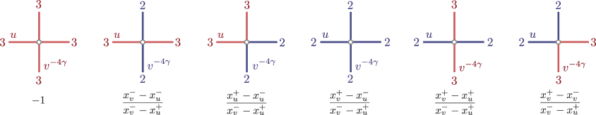
Figure 6: The new six nonzero vertices. They are used to evaluate the domain wall partition function ${\mathcal{DW}}_{N}(\{u\},\{v\})$.

Naturally, the domain wall partition function $\mathcal{DW}_{N}(\{u\},\{v\})$ inherits the properties of $\mathcal{P}_{N}(\{u\},\{v\})$ with small differences. We list them below,

1. ${\mathcal{DW}}_{1}(\{u_{1}\},\{v_{1}\})=\frac{x^{+}_{u_{1}}-x^{-}_{u_{1}}}{x^{-}_{v_{1}}-x^{+}_{u_{1}}}\,,$

2. ${\mathcal{DW}}_{N}(\{u\},\{v\})=-\frac{x^{+}_{v_{i+1}}-x^{-}_{v_{i}}}{x^{-}_{v_{i+1}}-x^{+}_{v_{i}}}\,{\mathcal{DW}}_{N}(\{u\},\{v_{1},\ldots,v_{i+1},v_{i}\ldots,v_{N}\})\,,$

3. ${\mathcal{DW}}_{N}(\{u\},\{v\})=-\frac{x^{+}_{u_{i+1}}-x^{-}_{u_{i}}}{x^{-}_{u_{i+1}}-x^{+}_{u_{i}}}\,{\mathcal{DW}}_{N}(\{u_{1},\ldots,u_{i+1},u_{i},\ldots,u_{N}\},\{v\})\,,$

4. ${\mathcal{DW}}_{N}(\{u\},\{v\})\Big{|}_{x^{+}_{u_{N}}=x^{+}_{v_{N}}}=\,\,(-1)^{N-1}\frac{x^{+}_{u_{N}}-x^{-}_{u_{N}}}{x^{-}_{v_{N}}-x^{+}_{u_{N}}}\,\,\prod_{i=1}^{N-1}\frac{x^{+}_{v_{N}}-x^{-}_{u_{i}}}{x^{-}_{v_{N}}-x^{+}_{u_{i}}}\,\,{\mathcal{DW}}_{N-1}(\{u\},\{v\})\,.$

Property I is again trivial and follows from the weight of the third vertex of the figure 6. Properties II and III are consequence of the Yang-Baxter equation and can be shown in a similar fashion using the procedure described in figure 4(b), but this time using the $R$-matrix built out of the vertices of figure 6. Such $R$-matrix satisfies the unitary condition and the Yang-Baxter equation.

Property IV is a consequence of the weights of the vertices. In the square lattice of figure 4, there are only two allowed vertices at the intersection of the lines $\{u_{N},v_{N}\}$. The vertex with weight proportional to $x^{+}_{v}-x^{+}_{u}$ is zero when $x^{+}_{u_{N}}=x^{+}_{v_{N}}$. So there is only one possible nonzero vertex at this intersection and it is not difficult to see that the lines corresponding to $u_{N}$ and $v_{N}$ are frozen in this case and the fourth property above follows.

The solution for ${\mathcal{DW}}_{N}(\{u\},\{v\})$ is given in a completely factorized form as follows

$${\mathcal{DW}}_{N}(\{u\},\{v\})=\prod^{N}_{i,j}\frac{1}{(x^{-}_{v_{i}}-x^{+}_{u_{j}})}\prod_{i=1}^{N}(x^{+}_{u_{i}}-x^{-}_{u_{i}})\prod_{j>i}^{N}(x^{+}_{v_{j}}-x^{-}_{v_{i}})\prod_{j>i}^{N}(x^{+}_{u_{j}}-x^{-}_{u_{i}})\,.$$ (3.10)

We will now prove that the solution given above is unique. The proof is by induction. One can immediately see that the expression above satisfies the property I above. In addition, inspecting the weights of the vertices of figure 6, we see that the domain wall partition function has the form

$${\mathcal{DW}}_{N}(\{u\},\{v\})=(x^{+}_{u_{N}}-x^{-}_{u_{N}})\prod_{i}^{N}\frac{1}{(x^{-}_{v_{i}}-x^{+}_{u_{N}})}\,g(\{u\},\{v\})\,,$$ (3.11)

where $g(\{u\},\{v\})$ is a polynomial of degree $(N-1)$ in $x^{+}_{u_{N}}$. Suppose that ${\mathcal{DW}}_{N-1}$ is known. Using the property II and the result of property IV, we can derive recursion relations for $x^{+}_{u_{N}}=x^{+}_{v_{i}}$ for $i=1,\ldots,N$. These are $N$ conditions that uniquely fix $g(\{u\},\{v\})$ and consequently the domain wall partition function.

The result for the domain wall partition function that we have just proven enables us to find an expression for the partition function $\mathcal{P}_{N}(\{u\},\{v\})$ which is proportional to the matrix part of the hexagon form-factor of (3.8). Substituting $\mathcal{P}_{N}(\{u\},\{v\})$, we get that

$$h_{\mathnormal{\Psi}_{1}\ldots\mathnormal{\Psi}_{N}|\bar{\mathnormal{\Psi}}_{1}\ldots\bar{\mathnormal{\Psi}}_{N}}(\{u\},\{v\})=\frac{\prod_{i=1}^{N}\prod_{j=1}^{N}h_{\mathnormal{\Psi}|\bar{\mathnormal{\Psi}}}(u_{i},v_{j})}{\prod_{i>j}h_{\mathnormal{\Psi}|\bar{\mathnormal{\Psi}}}(u_{i},u_{j})\prod_{i>j}h_{\mathnormal{\Psi}|\bar{\mathnormal{\Psi}}}(v_{i},v_{j})}\,.$$ (3.12)

Using a similar reasoning, one can also derive the form-factor $h_{\bar{\mathnormal{\Psi}}_{1}\ldots\bar{\mathnormal{\Psi}}_{N}|\mathnormal{\Psi}_{1}\ldots\mathnormal{\Psi}_{N}}$. That simply amounts to exchanging $\bar{\mathnormal{\Psi}}\leftrightarrow\mathnormal{\Psi}$ on the right hand side of the expression above. This is the main result of this section. In what follows, we proceed to the computation of the full three-point function.

3.2.2 The three-point functions

We consider now the full three-point function in the setup of figure 3, in which the excitations of the operator $\mathcal{O}_{1}$ and $\mathcal{O}_{2}$ are parametrized by the set of rapidities $\{u\}$ and $\{v\}$ respectively. We will be working in the asymptotic regime where all the lengths involved (both $L_{i}$ and $l_{ij}$) are large and all the finite size corrections can be neglected. According to the hexagon program, the asymptotic three-point function of these operators at any loop order is given by

$$\left(\frac{C^{\rm{asym}}_{\bullet\bullet\circ}(N)}{C_{\circ\circ\circ}}\right)^{2}=\frac{\prod_{i=1}^{N}\,\mu_{\mathnormal{\Psi}}(u_{i})\,\mu_{\mathnormal{\Psi}}(v_{i})}{\prod\limits_{y=u,v}\Bigl{(}{\rm{det}}\,\partial_{y_{i}}\phi_{y_{j}}\prod\limits_{i<j}S_{\mathfrak{su}(1|1)}(y_{i},y_{j})\Bigr{)}}\times\mathcal{B}(N)^{2}\,,$$ (3.13)

with

$$\mathcal{B}(N)=\underset{\beta\cup\bar{\beta}=\{v\}}{\underset{\alpha\cup\bar{\alpha}=\{u\}}{\sum}}(-1)^{X}\,w_{l_{13}}(\alpha,\bar{\alpha})\,w_{l_{12}}(\beta,\bar{\beta})\,h_{\mathnormal{\Psi}_{1}\ldots\mathnormal{\Psi}_{|\alpha|}|\bar{\mathnormal{\Psi}}_{1}\ldots\bar{\mathnormal{\Psi}}_{|\beta|}}(\alpha,\beta)\,h_{\bar{\mathnormal{\Psi}}_{1}\ldots\bar{\mathnormal{\Psi}}_{|\bar{\beta}|}|\mathnormal{\Psi}_{1}\ldots\mathnormal{\Psi}_{|\bar{\alpha}|}}(\bar{\beta},\bar{\alpha})\,.$$ (3.14)

Moreover, $C_{\circ\circ\circ}$ is the three-point function of the three BPS operators obtained when $N=0$ and it is a constant combinatorial factor. The function $\mu_{\mathnormal{\Psi}}(u)$ is the measure and as explained in [4] its square root gives the correct normalization of the one-particle state in the hexagon program. It is defined by

$$\mu_{\mathnormal{\Psi}}(u)=\frac{i}{\underset{u=v}{{\rm{residue}}}\,\,h_{\mathnormal{\Psi}|\bar{\mathnormal{\Psi}}}(u,v)}\,.$$ (3.15)

The phase $\phi_{u}$ in (3.13) is given by

$$e^{i\phi_{u_{j}}}\equiv e^{ip_{u_{j}}L_{1}}\prod_{i\neq j}^{N_{1}}(-S_{\mathfrak{su}(1|1)}(u_{j},u_{k}))\,,$$ (3.16)

and the phase $\phi_{v}$ is defined similarly. The determinant of the derivative of the phase $\phi_{u}$ is the usual Gaudin norm.

The hexagon form-factors appearing in (3.14) are evaluated in the spin-chain frame and they are nonzero only when $|\alpha|=|\beta|$. Moreover, $w_{l}$ are splitting factors, generically defined for a partition $\gamma\cup\bar{\gamma}$ of a set of rapidities $\{w\}$ by

$$w_{l}(\gamma,\bar{\gamma})=\prod_{w_{j}\in\bar{\gamma}}\left(a_{l}(w_{j})\prod_{w_{i}\in\gamma\,,\,i>j}S_{\mathfrak{su}(1|1)}(w_{j},w_{i})\right)\,,\quad\quad{\rm with}\quad\quad a_{l}(w)=e^{ip(w)l}\,.$$ (3.17)

In the spin-chain frame normalization, the all-loop spin-chain $\mathfrak{su}(1|1)$ $S$-matrix is given by

$$S_{12}|_{{\rm{spin}}}\,|\chi_{1}^{3\dot{1}}\chi_{2}^{3\dot{1}}\rangle=-(S^{0}_{12})^{2}A_{12}|_{{\rm{spin}}}\,|\chi_{2}^{3\dot{1}}\chi_{1}^{3\dot{1}}\rangle\equiv S_{\mathfrak{su}(1|1)}|\chi_{2}^{3\dot{1}}\chi_{1}^{3\dot{1}}\rangle\,,$$ (3.18)

where

$$(S^{0}_{12})^{2}(u_{1},u_{2})=\frac{u_{1}-u_{2}+i}{u_{1}-u_{2}-i}\frac{(1-1/x_{1}^{-}x^{+}_{2})^{2}}{(1-1/x_{1}^{+}x^{-}_{2})^{2}}\frac{1}{\sigma^{2}(u_{1},u_{2})}\,,\quad\quad A_{12}|_{{\rm{spin}}}=\frac{x_{2}^{+}-x_{1}^{-}}{x_{2}^{-}-x_{1}^{+}}\,.$$

The expression (3.14) explicitly depends on the two lengths $l_{13}$ and $l_{12}$. It is possible to use the Bethe equations for the operator $\mathcal{O}_{1}$ (the unusual signs below appear because the excitations are fermionic),

$$a_{L_{1}}(u_{j})\prod_{i\neq j}^{N_{1}}\left(-S_{\mathfrak{su}(1|1)}(u_{j},u_{i})\right)=1\,,\quad\quad j=1,\ldots,N_{1}\,,$$ (3.19)

and rewrite it in terms of the length $l_{12}$ only. After that, one gets at tree-level the scalar product of two off-shell $\mathfrak{su}(1|1)$ states.

In the expression (3.14) above, $(-1)^{X}$ accounts for some sign differences between the two hexagons involved in the structure constant. It was already noticed in [4], that such signs were important in order to get a match with both weak and strong coupling data. The empirical rule found there was to include the factor $(-1)^{M}$, where $M$ is nothing but the total number of magnons of the second hexagon (equivalently $M=|\bar{\alpha}|+|\bar{\beta}|$). In a similar way, we have found the need of introducing additional signs to get an agreement with the tree-level data. In total, we have that

$$X=|\bar{\alpha}|N\,.$$ (3.20)

Note that $M$ should be always even in order to get a nonzero hexagon so that $(-1)^{M}$ does not introduce any sign.

The two particle fermionic hexagon form-factor is related to $S_{\mathfrak{su}(1|1)}$. By explicitly evaluating the hexagon form factors for $N=1$ in the spin-chain frame, one can check that the following identity holds

$$\frac{h_{\mathnormal{\Psi}|\bar{\mathnormal{\Psi}}}(u,v)}{h_{\mathnormal{\Psi}|\bar{\mathnormal{\Psi}}}(v,u)}=S_{\mathfrak{su}(1|1)}(u,v).$$ (3.21)

This identity reflects the Watson equation for form-factors which is, by construction, automatically satisfied by the hexagon ansatz. Using this relation, we can write the three-point function in a more concise way. Given two sets $\rho_{u}=\{u_{1},\dots,u_{|\rho_{u}|}\}$ and $\rho_{v}=\{v_{1},\dots,v_{|\rho_{v}|}\}$, let us introduce the notation

$$e^{ip_{\rho_{u}}l}=\prod_{i}e^{ip(u_{i})\,l}\,,\,\,\,\,\,h_{\mathnormal{\Psi}|\bar{\mathnormal{\Psi}}}(\rho_{u},\rho_{v})=\prod_{i,j}h_{\mathnormal{\Psi}|\bar{\mathnormal{\Psi}}}(u_{i},v_{j})\,,$$ (3.22)

$$h^{>}_{\mathnormal{\Psi}|\bar{\mathnormal{\Psi}}}(\rho_{u},\rho_{v})=\prod_{i>j}h_{\mathnormal{\Psi}|\bar{\mathnormal{\Psi}}}(u_{i},v_{j})\,,\,\,\,\,\,h^{<}_{\mathnormal{\Psi}|\bar{\mathnormal{\Psi}}}(\rho_{u},\rho_{v})=\prod_{i<j}h_{\mathnormal{\Psi}|\bar{\mathnormal{\Psi}}}(u_{i},v_{j})\,.$$ (3.23)

The equation (3.14) can then be rewritten as

$$\mathcal{B}(N)=\underset{\beta\cup\bar{\beta}=\{v\}}{\underset{\alpha\cup\bar{\alpha}=\{u\}}{\sum}}(-1)^{X}\,\frac{e^{ip_{\bar{\alpha}}l_{13}+ip_{\bar{\beta}}l_{12}}\,\,h^{<}_{\mathnormal{\Psi}|\bar{\mathnormal{\Psi}}}(\bar{\alpha},\alpha)h^{<}_{\mathnormal{\Psi}|\bar{\mathnormal{\Psi}}}(\bar{\beta},\beta)h_{\mathnormal{\Psi}|\bar{\mathnormal{\Psi}}}(\alpha,\beta)h_{\bar{\mathnormal{\Psi}}|\mathnormal{\Psi}}(\bar{\beta},\bar{\alpha})}{h^{>}_{\mathnormal{\Psi}|\bar{\mathnormal{\Psi}}}(\alpha,\bar{\alpha})h^{>}_{\mathnormal{\Psi}|\bar{\mathnormal{\Psi}}}(\beta,\bar{\beta})h^{>}_{\mathnormal{\Psi}|\bar{\mathnormal{\Psi}}}(\alpha,\alpha)h^{>}_{\mathnormal{\Psi}|\bar{\mathnormal{\Psi}}}(\beta,\beta)h^{>}_{\bar{\mathnormal{\Psi}}|\mathnormal{\Psi}}(\bar{\alpha},\bar{\alpha})h^{>}_{\bar{\mathnormal{\Psi}}|\mathnormal{\Psi}}(\bar{\beta},\bar{\beta})}\,.$$ (3.24)

Let us now further expand on the comparison with data. In subsection 2.2, a determinant expression for the three-point function of three generic $\mathfrak{su}(1|1)$ operators at tree-level was derived, see (2.16) and (LABEL:determinant). This result, more precisely $C_{123}/\mathcal{R}$ with $N_{3}=0$ and with a suitable normalization of the wave-functions, can be compared with the tree-level limit of $\mathcal{B}(N)$. One way of finding the relevant normalization of the wave-functions is by comparing the two results for the simplest case $N=1$. In this section, all the hexagon form-factors are evaluated in the spin-chain frame and at order $g^{0}$, one has

$$h_{\mathnormal{\Psi}|\bar{\mathnormal{\Psi}}}(u,v)=-h_{\bar{\mathnormal{\Psi}}|\mathnormal{\Psi}}(u,v)=\frac{1}{u-v}\;,\quad\quad S_{su(1|1)}(u_{i},u_{j})=-1\,,$$ (3.25)

and

$$\mathcal{B}(1)=\frac{1}{u-v}\,(1-e^{ip(v)l_{12}}\,e^{ip(u)l_{13}})\,.$$ (3.26)

Using the Bethe equation for the operator $\mathcal{O}_{1}$, it is not difficult to see that the result above agrees with the result for $C_{123}/\mathcal{R}$ given in (2.16) if we multiply this later by the normalization factor $\mathcal{N}(u)\times\mathcal{N}(v)$ where $\mathcal{N}$ is given by

$$\mathcal{N}(u)=\sqrt{i}\,(e^{-ip(u)}-1)\,.$$ (3.27)

In this way, we have found the correct normalization of the wave-functions to compare the two results. We should then multiply the wave-function given in (2.10) by these normalization factors for all rapidities. One can now evaluate $\mathcal{B}(N)$ for different values of $N$ and check that in fact it reproduces the results obtained from the determinant formula. Alternatively, one can directly compare the complete $C_{123}$ given in (2.16) computed with standard normalized wave-functions with the properly normalized structure constants computed with the hexagon program as in (3.13).

We have seen that the factor $\mathcal{B}(N)$ of the tree-level structure constant can be written as a determinant, which is directly related to the fact that the scalar product of two off-shell $\mathfrak{su}(1|1)$ states can also be written in the form of a determinant, see also [29, 30]. This property appears to be special to $\mathfrak{su}(1|1)$ and it is currently not known if such determinant expressions exist in the other rank one sectors, namely $\mathfrak{su}(2)$ and $\mathfrak{sl}(2)$. A natural question is whether $\mathcal{B}(N)$ can still be written as a determinant (or in another computationally efficient form) when loop corrections are included. We have not found a full answer to this question, but in what follows we will show that at strong coupling leading order such simplification exists and the result can be indeed expressed in the form of a determinant.

Strong coupling limit

As a prediction for a direct strong coupling computation of the asymptotic three-point functions considered in this section, we consider the large coupling limit of (3.24). There are several regimes in the kinematical space and here we focus on the so-called BMN regime for which the momentum scales as $p\sim 1/g$ and the rapidities scales as $u\sim g$. Using that in this regime

$$x_{u}^{\pm}=x_{u}\pm\frac{i\,x_{u}\,p_{u}}{2}+\mathcal{O}(1/g^{2})\,,$$ (3.28)

and the leading expression for the dressing phase, i.e. the AFS dressing factor of [31, 32], it is simple to derive that

$$h_{\mathnormal{\Psi}|\bar{\mathnormal{\Psi}}}(u,v)=\frac{\sqrt{p_{u}\,p_{v}\,x_{u}x_{v}}}{x_{u}-x_{v}}+\mathcal{O}(1/g^{2})\,.$$ (3.29)

When we plug this expression in (3.14) and use the fact that

$$S_{\mathfrak{su}(1|1)}(u,v)\simeq-1+\mathcal{O}(1/g)\,,\quad\quad{\rm{and}}\quad\quad L_{i}\sim g\,,$$ (3.30)

where the condition on $L_{i}$ is necessary in order for the operators to satisfy the Bethe equations (3.19), we obtain after a little massaging that the factor $\mathcal{B}(N)$ contributing to the strong coupling structure constant can be expressed as

$$\mathcal{B}(N)= \sqrt{\prod_{i=1}^{N}p_{u_{i}}p_{v_{i}}x_{u_{i}}x_{v_{i}}}\underset{\beta\cup\bar{\beta}=\{v\}}{\underset{\alpha\cup\bar{\alpha}=\{u\}}{\sum}}(-1)^{X}\,\,(-1)^{P_{\alpha}+P_{\beta}}\,e^{ip_{\bar{\alpha}}l_{13}+ip_{\bar{\beta}}l_{12}}\,\frac{g^{\alpha\alpha}_{>}\,g^{\beta\beta}_{>}\,g^{\bar{\alpha}\bar{\alpha}}_{>}\,g^{\bar{\beta}\bar{\beta}}_{>}}{g^{\alpha\beta}g^{\bar{\alpha}\bar{\beta}}}\,,$$ (3.31)

where $(-1)^{P_{\alpha}}$ is defined as the sign of permutation of the ordered set $\{u\}$ which gives $\alpha\cup\bar{\alpha}$. In this expression, we use that $g^{\alpha\beta}=\underset{u_{i}\in\alpha,v_{j}\in\beta}{\prod}(x_{u_{i}}-x_{v_{j}})$ and $g^{\alpha\alpha}_{>}=\underset{i>j}{\underset{u_{i},u_{j}\in\alpha}{\prod}}(x_{u_{i}}-x_{u_{j}})$ .

This formula can be finally recasted as the following determinant

$$\mathcal{B}(N)=(-1)^{\frac{N(N-1)}{2}}\sqrt{\prod_{i=1}^{N}p_{u_{i}}p_{v_{i}}x_{u_{i}}x_{v_{i}}}\,\det_{1\leq i,j\leq N}\left[\frac{1-e^{ip_{u_{i}}l_{13}+ip_{v_{j}}l_{12}}}{x_{u_{i}}-x_{v_{j}}}\right]\,.$$ (3.32)

To compute the properly normalized structure constant of (3.13) in the strong coupling limit, we also need to find the leading contribution both of the measure $\mu_{\mathnormal{\Psi}}(u)$ and the Gaudin norm at large coupling. Using the result (3.29) for $h_{\mathnormal{\Psi}|\bar{\mathnormal{\Psi}}}(u,v)$ and the definition of the measure $\mu_{\mathnormal{\Psi}}(u)$ of (3.15), it is not difficult to see that

$$\mu_{\mathnormal{\Psi}}(u)=i\frac{\partial_{u}x_{u}}{p_{u}x_{u}}+\mathcal{O}(1/g)\,.$$ (3.33)

The Gaudin norms can be evaluated using the definition of the phases $\phi_{u_{j}}$ given in (3.16) and the $S_{\mathfrak{su}(1|1)}(u,v)$ of (3.30), leading to

$${\rm{det}}\,\partial_{u_{i}}\phi_{u_{j}}=\prod_{i=1}^{N}\partial_{u_{i}}p_{u_{i}}L_{1}+\mathcal{O}(1/g^{N+1})\,,$$ (3.34)

and the result for ${\rm{det}}\,\partial_{v_{i}}\phi_{v_{j}}$ is analogous to the one above with both $u_{i}$ and $L_{1}$ replaced by $v_{i}$ and $L_{2}$ respectively.

The strong coupling limit of the structure constants $C^{\rm{asym}}_{\bullet\bullet\circ}(N)$ of (3.13) can then be obtained by assembling together these results. By analyzing how these several contributions scale with $g$, it follows that the structure constants are of order $\mathcal{O}(1)$ in the coupling for any $N$.

3.3 The 3 non-BPS case

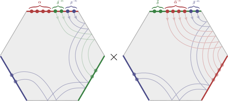
Figure 7: The product of two hexagons is the core of the three-point function. We divide each set of excitations in three partitions and distribute them over the two form-factors. Two out of the three sets are mirror transformed which is equivalent to transfer the excitations to the other physical edges.

In this subsection, we will compare the results for the three-point functions of three $\mathfrak{su}(1|1)$ non-BPS operators obtained in [14] at one-loop order by a direct perturbative calculation with the results predicted by the hexagon program. This constitutes a rather nontrivial test of the hexagon program.

In [14], we have considered a setup consisting of three operators in the $\mathfrak{su}(1|1)$, where $\mathcal{O}_{1}$ was made out of $Z\equiv\mathnormal{\Phi}^{34}$ and $\mathnormal{\Psi}\equiv\psi_{\alpha=1}^{4}$ and $\mathcal{O}_{2}$ was made out of the corresponding conjugate fields $\bar{Z}=(Z)^{*}$ and $\bar{\mathnormal{\Psi}}\equiv(\mathnormal{\Psi})^{\dagger}$. The third operator $\mathcal{O}_{3}$ was chosen to be a certain rotated operator in order to have a non-extremal three-point function. More specifically

$$\mathcal{O}_{3}=\frac{1}{(L_{3}-N_{3})!^{2}}\sum_{1\leq n_{1}<\ldots<n_{N_{3}}\leq L_{3}}\psi^{(3)}_{n_{1},n_{2},\ldots,n_{N_{3}}}\,(\mathfrak{R}^{2}_{\;\;4}\mathfrak{R}^{1}_{\;\;3})^{L_{3}-N_{3}}\cdot\mathop{\mathrm{Tr}}\,(Z\dots\underset{n_{1}}{\mathnormal{\Psi}}\dots\underset{n_{2}}{\mathnormal{\Psi}}\dots Z)\ \,,$$ (3.35)

where $\psi^{(3)}$ is the wave-function depending on the momenta of the excitations $\mathnormal{\Psi}$. Here $\mathfrak{R}^{a}_{\;\;b}$ are the $\mathfrak{su}(4)$ generators with $a,b=1,\ldots,4$. For all operators $\mathcal{O}_{i}$, $L_{i}$ and $N_{i}$ are the corresponding length and number of excitations.

At one-loop level, the corrections coming from both the wave-functions and Feynman diagrams were computed in [14]. This latter correction turned out to be encoded in the form of some splitting operators to be inserted on top of the tree-level contractions. When combined both corrections together we have found a remarkably simple factorized result given by

$$C_{\bullet\bullet\bullet}=\mathcal{C}\;\frac{\prod\limits_{k=1}^{3}\prod\limits_{\begin{subarray}{c}i<j\end{subarray}}^{N_{k}}f(y^{(k)}_{i},y^{(k)}_{j})}{\prod\limits_{i=1}^{N_{1}}\prod\limits_{j=1}^{N_{2}}f(y^{(1)}_{i},y^{(2)}_{j})}\prod\limits_{k=1}^{N_{1}}\left[1-(y^{(1)}_{k})^{L_{2}}\prod\limits_{i=1}^{N_{2}}\left(-S(y^{(2)}_{i},y^{(1)}_{k})\right)\right]\,,$$ (3.36)

where we are using the notation $y^{(i)}_{k}=e^{ip^{(i)}_{k}}$, with $\{p^{(i)}_{k}\}_{k=1}^{N_{i}}$ being the set of momenta characterizing the excitations of the operator $\mathcal{O}_{i}$. The normalization factor $\mathcal{C}$ and $f$ are given by

$$\mathcal{C} =\prod_{i=1}^{3}\left(\frac{L_{i}}{\mathcal{N}^{(i)}}\right)^{1/2}\left[1+g^{2}\left(N_{3}^{2}-1\right)-\frac{1}{4}\sum_{i=1}^{3}\mathbb{\gamma}_{i}\right]\,,$$ (3.37)

$$f(s,t) =(s-t)\left[1-\frac{g^{2}}{2}\left(\frac{s}{t}+\frac{t}{s}-\frac{1}{s}-s-\frac{1}{t}-t+2\right)\right]\,.$$

with $\gamma_{i}$ being the anomalous dimension of the operator $\mathcal{O}_{i}$.

In order to compare the perturbative calculations with the results of the hexagon program, we have to properly normalize the wave-functions $\psi^{(i)}$. One way of finding the correct normalization is to use the results of the previous subsection for two non-BPS operators when $N=1$ and match it with the corresponding one-loop three-point function. Since the wave-functions only contain local information of each operator, they ought to be the same for any three-point function within the same sector. In order to compute the three-point function of one BPS and two non-BPS operators at one-loop we make use of the splitting insertions for fermions obtained in [14]. Once the comparison with $\mathcal{B}(1)$ of (3.14) at one-loop order is made, one finds that the two results agree if the one excitation wave-function is normalized as

$$\psi(n_{1})=\mathcal{N}(p)\,e^{ipn_{1}}\,,\quad{\rm{with}}\quad\quad\mathcal{N}(p)=\sqrt{i}\,\frac{(e^{-ip}-1)}{1+g^{2}(e^{ip}+e^{-ip}-2)}\,.$$ (3.38)

In the case of more than one excitation the normalized wave-function is obtained by multiplying it by $\mathcal{N}(p_{i})$ given above for all the excitations $i$.

We want now to access this three-point function within the framework of the hexagon program. In order to match our previous setup, we choose the set of excitations as follows: the physical edge associated to the operator $\mathcal{O}_{1}$ contains $N_{1}$ excitations of type $\mathnormal{\Psi}=\chi^{3\dot{1}}$, the edge corresponding to $\mathcal{O}_{2}$ has $N_{2}$ excitations of the type $\bar{\mathnormal{\Psi}}=\chi^{2\dot{4}}$ and remaining physical edge has $N_{3}=l_{23}=N_{2}-N_{1}$ excitations of type $\mathnormal{\Psi}=\chi^{3\dot{1}}$. For details about the construction of operators in the hexagon formalism, we refer the reader to the Appendix B of [4]. The relevant hexagon form-factor to be considered contains three sets of type of excitations. Accounting for the mirror transformations illustrated in figure 7, and given three generic sets of rapidities $\{u_{i}\}_{i=1}^{N_{u}},\{w_{i}\}_{i=1}^{N_{w}}$ and $\{v_{i}\}_{i=1}^{N_{v}}$ it reads

$$\mathfrak{h}_{\{u\},\{w\},\{v\}}\equiv(-1)^{N_{v}+N_{w}}h{\overbrace{{}^{3\dot{1},\ldots,3\dot{1},}}^{N_{u}}\overbrace{{}^{1\dot{3},\ldots,1\dot{3},}}^{N_{w}}\overbrace{{}^{2\dot{4},\ldots,2\dot{4}}}^{N_{v}}}(u_{1},\ldots,w^{-2\gamma}_{1},\ldots,v^{-4\gamma}_{1},\ldots),$$ (3.39)

where we are using the notations of (3.1) and the sign $(-1)^{N_{v}+N_{w}}$ comes from the crossing rules for the excitations as described in Appendix A. The full asymptotic three-point function is then built out of this hexagon form-factor through

$$\left(\frac{C^{\rm{asym}}_{\bullet\bullet\bullet}(N_{1},N_{3})}{C_{\circ\circ\circ}}\right)^{2}=\frac{\prod\limits_{i=1}^{N_{1}}\,\mu_{\mathnormal{\Psi}}(u_{i})\,\prod\limits_{i=1}^{N_{2}}\,\mu_{\mathnormal{\Psi}}(v_{i})\,\prod\limits_{i=1}^{N_{3}}\,\mu_{\mathnormal{\Psi}}(w_{i})}{\prod\limits_{y=u,v,w}\Bigl{(}{\rm{det}}\,\partial_{y_{i}}\phi_{y_{j}}\prod\limits_{i<j}S_{\mathfrak{su}(1|1)}(y_{i},y_{j})\Bigr{)}}\,\times\mathcal{C}(N_{1},N_{3})^{2}\,,$$ (3.40)

where $C_{\circ\circ\circ}$ is a constant combinatorial factor equal to the three-point function of the three BPS operators obtained when $N_{1}=N_{3}=0$. The functions $\mu_{\mathnormal{\Psi}}(u)$ and $\phi_{u_{i}}$ were defined in (3.15) and (3.16) respectively. Finally,

$$\mathcal{C}(N_{1},N_{3})=\underset{\delta\cup\bar{\delta}=\{w\}}{\underset{\beta\cup\bar{\beta}=\{v\}}{\underset{\alpha\cup\bar{\alpha}=\{u\}}{\sum}}}(-1)^{X}\,w_{l_{13}}(\alpha,\bar{\alpha})\,w_{l_{12}}(\beta,\bar{\beta})\,w_{l_{23}}(\delta,\bar{\delta})\,\mathfrak{h}_{\alpha,\delta,\beta}\,\mathfrak{h}_{\bar{\delta},\bar{\alpha},\bar{\beta}}\,,$$ (3.41)

with the splitting factors given in (3.17). Upon expanding $\mathcal{C}(N_{1},N_{3})$ above up to one-loop we have found that it matches with the properly normalized results referred to above, once $X$ is taken to be

$$X={|\bar{\delta}|N_{1}+|\bar{\alpha}|N_{2}+|\beta|N_{3}}\,.$$ (3.42)

Note that once again this differs from the rule advocated in [4] and mentioned in the previous section. It is desirable to have a deeper understanding of the origin of these relative signs between the hexagons.

4 Conclusions

In this paper, we have studied the three-point functions of operators in the $\mathfrak{su}(1|1)$ sector, i.e., containing a single type of fermionic excitations. We have managed to parametrize the most general configuration in this rank one sector by a sort of polarization vectors and showed that at leading order the structure constant can be expressed in the form of a determinant. In a particular limit, such determinant reduces to an off-shell scalar product of $\mathfrak{su}(1|1)$ Bethe states.

We have then applied the hexagon program of [4] to study all-loop correlators in this sector. We have started with the case of one BPS and two non-BPS operators. We have shown that the relevant hexagon form-factor can be identified with a domain wall partition function of a six-vertex model defined by some entries of the $\mathfrak{su}(2|2)$ $S$-matrix. This property appears to be specific for this sector and in particular, it is no longer true for other rank one sectors, where only at tree-level such identification can be made. A peculiar feature of the domain wall partition function we have found here is that it completely factorizes, see (3.12), and its computation becomes rather economical. We then assembled a pair of such completely factorized hexagon form-factors to compute the structure constants. Upon expanding it at leading order in the coupling constant we have checked that it matched precisely with our tree-level prediction once we include a relative sign factor between the two hexagons. This is an addition to the prescription put forward in [4], where it was already noticed the need of including some relative signs when the two hexagons are multiplied. This particular point certainly needs a clarification. The expression for the structure constants is given in (3.24) and one interesting limit of this expression is the strong coupling limit which is a prediction for a future string theory computation. We showed that in the BMN regime the structure constant admits surprisingly a determinant expression for any number of excitations. An interesting future direction that comes out of our results is to investigate the possibility of writing the full three-point function at finite coupling in a way that circumvents the computationally costly sums over partitions of Bethe roots. This is generally hard but within this particular setup where the hexagon form-factors are explicitly known, it might be a good starting point. Equally interesting is to take the classical limit of our result, for $L_{1},L_{2},N_{1},N_{2}\rightarrow\infty$ with $L_{i}/N_{i}$ fixed. Such limit for operators within the $\mathfrak{su}(2)$ sector was recently considered in [10].

We finally studied a particular configuration of three non-BPS operators in the same setup previously studied in [14] up to one-loop. We have managed to check that the structure constant computed from the hexagon program nicely reproduces the perturbative data of [14] once we include some relative signs between the two hexagons. This additional feature is analogous to the previous case. The one-loop structure constants computed in [14] have a completely factorized form even at one-loop. This raises hopes that it might be possible to find an all-loop simplification coming out of the hexagons. We hope to address this question in the future.

Appendix A The String Frame $\mathfrak{su}(2|2)$-invariant $S$-matrix

In this Appendix, we set our conventions for the string frame $\mathfrak{su}(2|2)$-invariant $S$-matrix. As explained in the main part of the paper, we evaluate the hexagon form-factors in the string frame and use the map between the frames to translate the results to the spin-chain frame when comparing with the available data. The string frame $S$-matrix obeys the standard Yang-Baxter equation and its action on the states does not produce $Z$ markers. The $S$-matrix has the following nonzero matrix elements ($\epsilon^{12}=\epsilon_{12}=1$)

$$S_{12}|\chi^{a}_{1}\chi^{b}_{2}\rangle=A_{12}|\chi^{\{a}_{2}\chi^{b\}}_{1}\rangle+B_{12}|\chi^{[a}_{2}\chi^{b]}_{1}\rangle+\frac{1}{2}C_{12}\epsilon^{ab}\epsilon_{\alpha\beta}|\chi_{2}^{\alpha}\chi_{1}^{\beta}\rangle\,,$$

$$S_{12}|\chi^{\alpha}_{1}\chi^{\beta}_{2}\rangle=D_{12}|\chi^{\{\alpha}_{2}\chi^{\beta\}}_{1}\rangle+E_{12}|\chi^{[\alpha}_{2}\chi^{\beta]}_{1}\rangle+\frac{1}{2}F_{12}\epsilon^{\alpha\beta}\epsilon_{ab}|\chi_{2}^{a}\chi_{1}^{b}\rangle\,,$$

$$S_{12}|\chi^{a}_{1}\chi^{\alpha}_{2}\rangle=G_{12}|\chi^{\alpha}_{2}\chi^{a}_{1}\rangle+H_{12}|\chi^{a}_{2}\chi^{\alpha}_{1}\rangle\,,\hskip 56.9055pt$$

$$S_{12}|\chi^{\alpha}_{1}\chi^{b}_{2}\rangle=K_{12}|\chi^{\alpha}_{2}\chi^{b}_{1}\rangle+L_{12}|\chi^{b}_{2}\chi^{\alpha}_{1}\rangle\,,\hskip 59.75078pt$$ (A.1)

where using the definitions

$$\eta_{i}=\eta(x_{i}^{+},x_{i}^{-})=e^{\frac{ip_{i}}{4}}\sqrt{i(x^{-}_{i}-x^{+}_{i})}\,,\quad\quad\tilde{\eta}_{1}=\eta_{1}\,e^{\frac{ip_{2}}{2}}\,,\quad\quad\tilde{\eta}_{2}=\eta_{2}\,e^{\frac{ip_{1}}{2}}\,,$$ (A.2)

the matrix elements are

$$A_{12}=\frac{x_{2}^{+}-x_{1}^{-}}{x_{2}^{-}-x_{1}^{+}}\frac{\tilde{\eta}_{2}\eta_{1}}{\eta_{2}\tilde{\eta}_{1}}\,,$$ (A.3)

$$B_{12}=\frac{x_{2}^{+}-x_{1}^{-}}{x_{2}^{-}-x_{1}^{+}}\left(1-2\frac{1-1/x_{2}^{-}x_{1}^{+}}{1-1/x_{2}^{+}x_{1}^{+}}\frac{x_{2}^{-}-x_{1}^{-}}{x_{2}^{+}-x_{1}^{-}}\right)\frac{\tilde{\eta}_{2}\eta_{1}}{\eta_{2}\tilde{\eta}_{1}}\,,$$ (A.4)

$$C_{12}=-\frac{2\eta_{1}\tilde{\eta}_{2}}{ix_{1}^{+}x_{2}^{+}}\frac{1}{1-1/x_{1}^{+}x_{2}^{+}}\frac{x_{2}^{-}-x_{1}^{-}}{x_{2}^{-}-x_{1}^{+}}\,,$$ (A.5)

$$D_{12}=-1\,,$$ (A.6)

$$E_{12}=-\left(1-2\frac{1-1/x^{+}_{2}x_{1}^{-}}{1-1/x^{-}_{2}x^{-}_{1}}\frac{x_{2}^{+}-x_{1}^{+}}{x_{2}^{-}-x^{+}_{1}}\right)\,,$$ (A.7)

$$F_{12}=\frac{2i(x_{1}^{+}-x_{1}^{-})(x_{2}^{+}-x_{2}^{-})}{\tilde{\eta}_{1}\eta_{2}\,x_{1}^{-}x_{2}^{-}}\frac{1}{1-1/x_{1}^{-}x_{2}^{-}}\frac{x_{2}^{+}-x_{1}^{+}}{x_{2}^{-}-x_{1}^{+}}\,,$$ (A.8)

$$G_{12}=\frac{x_{2}^{+}-x_{1}^{+}}{x_{2}^{-}-x_{1}^{+}}\frac{\eta_{1}}{\tilde{\eta}_{1}}\,,$$ (A.9)

$$H_{12}=\frac{x_{2}^{+}-x_{2}^{-}}{x_{2}^{-}-x_{1}^{+}}\frac{\eta_{1}}{\eta_{2}}\,,$$ (A.10)

$$K_{12}=\frac{x_{1}^{+}-x_{1}^{-}}{x_{2}^{-}-x_{1}^{+}}\frac{\tilde{\eta}_{2}}{\tilde{\eta}_{1}}\,,$$ (A.11)

$$L_{12}=\frac{x_{2}^{-}-x_{1}^{-}}{x_{2}^{-}-x_{1}^{+}}\frac{\tilde{\eta}_{2}}{\eta_{2}}\,.$$ (A.12)

One of the reasons to evaluate the hexagon form-factors using the string frame $S$-matrix is the fact that all the branch cut ambiguities of the function $\eta_{i}$ can be resolved by the variable $z$ parametrizing the rapidity torus [33, 20, 34]. This means also that there is no ambiguities when one performs crossing transformations. The way the variables transform will be explained in the next subsection. Using these crossing transformations, we have checked that the hexagon form-factors have all the expected properties such as invariance under cyclic rotations and consistency between all possible ways to move all the particles to a single physical edge. Using the variable $z$ corresponds to choosing a branch for the square roots in $\eta_{i}$.

A.1 Mirror transformations of fermions

The prescription to evaluate the hexagon form-factor in the case where not all the physical excitations are in one edge is to perform crossing transformations and move all of them to a single physical edge. The string frame $\mathfrak{su}(2|2)$ $S$-matrix is a meromorphic function when written in terms of a complex coordinate $z$ parametrizing the rapitidy torus. A crossing transformation, denoted by $2\gamma$ in what follows, corresponds to shift $z$ by half of the imaginary period of the torus. The transformation of the matrix elements of the $S$-matrix under crossing can be deduced using the following transformations

$$\eta_{i}^{-2\gamma}=-\frac{i\eta_{i}}{x_{i}^{+}}\,,\quad\quad\eta_{i}^{2\gamma}=\frac{i\eta_{i}}{x_{i}^{+}}\,,\quad\quad(x_{i}^{-})^{\pm 2\gamma}=\frac{1}{x_{i}^{-}}\,,\quad\quad(x_{i}^{+})^{\pm 2\gamma}=\frac{1}{x_{i}^{+}}\,,$$ (A.13)

where $\eta_{i}$ is defined in (A.2). In addition, it is also necessary to know how the fundamental excitations transform under crossing. According to Appendix D of [4], the fundamental excitations decompose as follows under the diagonal $\mathfrak{psu}(2|2)_{D}$ symmetry preserved by the hexagon

$$\chi^{A\dot{B}}(u)\,\,\mapsto\,\,\chi^{A}_{D}(u)\,\chi^{\dot{B}}_{D}(u^{-2\gamma})\,.$$ (A.14)

Moreover, one can also find in the Appendix D of [4] the relations

$$\chi^{a}(u^{2\gamma})=-\chi^{a}(u^{-2\gamma})\,,\quad\quad\chi^{\alpha}(u^{2\gamma})=\chi^{\alpha}(u^{-2\gamma})\,.$$ (A.15)

Using the above equations, one can deduce the transformations of the fundamental excitations. For example, one has

$$\chi^{\alpha\dot{a}}\,\overset{2\gamma}{\rightarrow}\,\chi^{a\dot{\alpha}}\,,\,\,\quad\chi^{a\dot{\alpha}}\,\overset{2\gamma}{\rightarrow}\,-\chi^{\alpha\dot{a}}\,,\,\,\quad\chi^{\alpha\dot{a}}\,\overset{-2\gamma}{\rightarrow}\,-\chi^{a\dot{\alpha}}\,,\quad\,\,\chi^{a\dot{\alpha}}\,\overset{-2\gamma}{\rightarrow}\,\chi^{\alpha\dot{a}}\,.$$ (A.16)

A.2 String and spin chain frames

In this paper, we compared the predictions for the structure constants obtained using the hexagon program with the available weak coupling data. Thus, it will be convenient to use the spin-chain frame instead of the string frame. There is a map between the excitations in one frame to the other and our strategy will be to evaluate the hexagon form factor in the string frame using the definitions and crossing rules given above and apply the map to the final result. Choosing the spin-chain frame parameters conveniently, the map for derivatives $D$, scalars $\mathnormal{\Phi}$ and fermions $\mathnormal{\Psi}$ is [4, 8]

$$D_{{\rm{string}}}=D_{{\rm{spin}}}\,,\quad\mathnormal{\Phi}_{{\rm{string}}}=Z^{\frac{1}{2}}\mathnormal{\Phi}_{{\rm{spin}}}Z^{\frac{1}{2}}\,,\quad\mathnormal{\Psi}_{{\rm{string}}}=Z^{\frac{1}{4}}\mathnormal{\Psi}_{{\rm{spin}}}Z^{\frac{1}{4}}\,,\quad$$ (A.17)

where $Z$ is the $Z$ marker.

As a consequence of the map above, the hexagon form-factors computed in the string frame can differ from the ones computed in the spin-chain frame only by a phase that depends on the momenta of the excitations. Using both the rule to pass the $Z$ markers from the right to the left of an excitation and replacing the $Z$ markers on the left of all excitations by their eigenvalues, it is possible to derive an expression for this phase, see [4] for details. In this work, we are interested in operators with fermionic excitations, so we are only going to give the expression for the phase in this case. The expression is a generalization of the one in [4] for scalars and the derivation is similar. Consider that the upper edge of the hexagon has $N_{1}$ physical excitations with momenta $p^{(1)}_{i}$. In addition, consider that the next physical edge moving anticlockwise has $N_{2}$ excitations with momenta $p^{(2)}_{j}$ and the remaining physical edge has $N_{3}$ excitations with momenta $p^{(3)}_{k}$. For this configuration, one has

$$h(N_{1},p^{(1)}_{i};N_{2},p^{(2)}_{j};N_{3},p^{(3)}_{k})_{{\rm{string}}}=F_{p^{(1)}}F_{p^{(2)}}F_{p^{(3)}}\times\hskip 71.13188pt$$ (A.18)

$$e^{-\frac{i}{4}[P^{(1)}(N_{1}+N_{3}-N_{2})+P^{(2)}(N_{2}+N_{1}-N_{3})+P^{(3)}(N_{3}+N_{2}-N_{1})]}\,\,h(N_{1},p^{(1)}_{i};N_{2},p^{(2)}_{j};N_{3},p^{(3)}_{k})_{{\rm{spin}}}\,,$$

where $h$ means hexagon form-factor, $P^{(i)}$ is the total momentum of the excitations $i$ and

$$F_{p^{(i)}}=\prod_{j=1}^{N_{i}}e^{\frac{ip^{(i)}_{j}}{2}(N_{i}+\frac{1}{2}-j)}\,.$$ (A.19)

References

- [1] K. Okuyama and L. S. Tseng, “Three-point functions in N = 4 SYM theory at one-loop,” JHEP 0408, 055 (2004) [hep-th/0404190].
- [2] R. Roiban and A. Volovich, “Yang-Mills correlation functions from integrable spin chains,” JHEP 0409 (2004) 032 [hep-th/0407140].
- [3] J. Escobedo, N. Gromov, A. Sever and P. Vieira, “Tailoring Three-Point Functions and Integrability,” JHEP 1109 (2011) 028 [arXiv:1012.2475 [hep-th]].
- [4] B. Basso, S. Komatsu and P. Vieira, “Structure Constants and Integrable Bootstrap in Planar N=4 SYM Theory,” arXiv:1505.06745 [hep-th].
- [5] B. Eden and A. Sfondrini, “Three-point functions in SYM: the hexagon proposal at three loops,” arXiv:1510.01242 [hep-th].
- [6] B. Basso, V. Goncalves, S. Komatsu and P. Vieira, “Gluing Hexagons at Three Loops,” arXiv:1510.01683 [hep-th].
- [7] Y. Jiang and A. Petrovskii, “Diagonal form factors and hexagon form factors,” arXiv:1511.06199 [hep-th].
- [8] Y. Jiang, “Diagonal Form Factors and Hexagon Form Factors II. Non-BPS Light Operator,” arXiv:1601.06926 [hep-th].
- [9] Y. Kazama, S. Komatsu and T. Nishimura, “Classical Integrability for Three-point Functions: Cognate Structure at Weak and Strong Couplings,” arXiv:1603.03164 [hep-th].
- [10] Y. Jiang, S. Komatsu, I. Kostov and D. Serban, “Clustering and the Three-Point Function,” arXiv:1604.03575 [hep-th].
- [11] G. M. Sotkov and R. P. Zaikov, “Conformal Invariant Two Point and Three Point Functions for Fields with Arbitrary Spin,” Rept. Math. Phys. 12, 375 (1977).
- [12] G. M. Sotkov and R. P. Zaikov, “On the Structure of the Conformal Covariant Point Functions,” Rept. Math. Phys. 19, 335 (1984).
- [13] M. S. Costa, J. Penedones, D. Poland and S. Rychkov, “Spinning Conformal Correlators,” JHEP 1111, 071 (2011) [arXiv:1107.3554 [hep-th]].
- [14] J. Caetano and T. Fleury, “Three-point functions and spin chains,” JHEP 1409 (2014) 173 [arXiv:1404.4128 [hep-th]].
- [15] V. E. Korepin, “Calculation of Norms of Bethe Wave Functions,” Commun. Math. Phys. 86 (1982) 391.
- [16] N. A. Slavnov, “Calculation of scalar products of wave functions and form factors in the framework of the algebraic Bethe ansatz,” Theoretical and Mathematical Physics 79, Number 2, 502-508.
- [17] M. Wheeler, “Scalar products in generalized models with SU(3)-symmetry,” Commun. Math. Phys. 327 (2014) 737 [arXiv:1204.2089 [math-ph]].
- [18] Y. Kazama, S. Komatsu and T. Nishimura, “Novel construction and the monodromy relation for three-point functions at weak coupling,” JHEP 1501, 095 (2015) Erratum: [JHEP 1508, 145 (2015)] [arXiv:1410.8533 [hep-th]].
- [19] G. Arutyunov, S. Frolov and M. Zamaklar, “The Zamolodchikov-Faddeev algebra for AdS(5) x S**5 superstring,” JHEP 0704 (2007) 002 [hep-th/0612229].
- [20] G. Arutyunov and S. Frolov, “Foundations of the Superstring. Part I,” J. Phys. A 42 (2009) 254003 [arXiv:0901.4937 [hep-th]].
- [21] N. Beisert et al., “Review of AdS/CFT Integrability: An Overview,” Lett. Math. Phys. 99 (2012) 3 [arXiv:1012.3982 [hep-th]].
- [22] N. Beisert, B. Eden and M. Staudacher, “Transcendentality and Crossing,” J. Stat. Mech. 0701 (2007) P01021 [hep-th/0610251].
- [23] N. Beisert, “The SU(2—2) dynamic S-matrix,” Adv. Theor. Math. Phys. 12 (2008) 948 [hep-th/0511082].
- [24] N. Beisert, “The Analytic Bethe Ansatz for a Chain with Centrally Extended su(2—2) Symmetry,” J. Stat. Mech. 0701 (2007) P01017 [nlin/0610017 [nlin.SI]].
- [25] A. Garbali, “The domain wall partition for the Izergin-Korepin 19-vertex model at a root of unity,” [arXiv:1411.2903 [math-ph]].
- [26] O. Foda, “N=4 SYM structure constants as determinants,” JHEP 1203 (2012) 096 [arXiv:1111.4663 [math-ph]].
- [27] O. Foda, M. Wheeler and M. Zuparic, “Factorized domain wall partition functions in trigonometric vertex models,” J. Stat. Mech. 0710, P10016 (2007) [arXiv:0709.4540 [math-ph]].
- [28] O. Foda, M. Wheeler and M. Zuparic, “Two elliptic height models with factorized domain wall partition functions,” Foda, Wheeler and Zuparic, J. Stat. Mech. P02001 (2008) [arXiv:0711.3058 [math-ph]].
- [29] A. Hutsalyuk, A. Liashyk, S. Z. Pakuliak, E. Ragoucy and N. A. Slavnov, “Scalar products of Bethe vectors in models with symmetry 1. Super-analog of Reshetikhin formula,” arXiv:1605.09189 [math-ph].
- [30] A. Hutsalyuk, A. Liashyk, S. Z. Pakuliak, E. Ragoucy and N. A. Slavnov, “Scalar products of Bethe vectors in models with symmetry 2. Determinant representation,” arXiv:1606.03573 [math-ph].
- [31] G. Arutyunov, S. Frolov and M. Staudacher, “Bethe ansatz for quantum strings,” JHEP 0410 (2004) 016 [hep-th/0406256].
- [32] P. Vieira and D. Volin, “Review of AdS/CFT Integrability, Chapter III.3: The Dressing factor,” Lett. Math. Phys. 99 (2012) 231 [arXiv:1012.3992 [hep-th]].
- [33] G. Arutyunov and S. Frolov, “On String S-matrix, Bound States and TBA,” JHEP 0712 (2007) 024 [arXiv:0710.1568 [hep-th]].
- [34] R. A. Janik, “The AdS(5) x S**5 superstring worldsheet S-matrix and crossing symmetry,” Phys. Rev. D 73 (2006) 086006 [hep-th/0603038].