Learning from Multiway Data: Simple and Efficient Tensor Regression

Abstract

Tensor regression has shown to be advantageous in learning tasks with multi-directional relatedness. Given massive multiway data, traditional methods are often too slow to operate on or suffer from memory bottleneck. In this paper, we introduce subsampled tensor projected gradient to solve the problem. Our algorithm is impressively simple and efficient. It is built upon projected gradient method with fast tensor power iterations, leveraging randomized sketching for further acceleration. Theoretical analysis shows that our algorithm converges to the correct solution in fixed number of iterations. The memory requirement grows linearly with the size of the problem. We demonstrate superior empirical performance on both multi-linear multi-task learning and spatio-temporal applications.

1 Introduction

Massive multiway data emerge from many fields: space-time measurements on several variables in climate dynamics (Hasselmann, 1997), multichannel EEG signals in neurology (Acar et al., 2007) and natural images sequences in computer vision (Vasilescu & Terzopoulos, 2002). Tensor provides a natural representation for multiway data. In particular, tensor decomposition has been a popular technique for exploratory data analysis (Kolda & Bader, 2009) and has been extensively studied. In contrast, tensor regression, which aims to learn a model with multi-linear parameters, is especially suitable for applications with multi-directional relatedness, but has not been fully examined. For example, in a task that predicts multiple climate variables at different locations and time, the data can be indexed by variable $\times$ location $\times$ time. Tensor regression provides us with a concise way of modeling complex structures in multiway data.

Many tensor regression methods have been proposed (Zhao et al., 2011; Zhou et al., 2013; Romera-Paredes et al., 2013; Wimalawarne et al., 2014; Signoretto et al., 2014), leading to a broad range of successful applications ranging from neural science to climate research to social network analysis. These methods share the assumption that the model parameters form a high order tensor and there exists a low-dimensional factorization for the model tensor. They can be summarized into two types of approaches: (1) alternating least square (ALS) sequentially finds the factor that minimizes the loss while keeping others fixed; (2) spectral regularization approximates the original non-convex problem with a convex surrogate loss, such as the nuclear norm of the unfolded tensor.

A clear drawback of all the algorithms mentioned above is high computational cost. ALS displays unstable convergence properties and outputs sub-optimal solutions (Cichocki et al., 2009). Trace-norm minimization suffers from slow convergence (Gandy et al., 2011). Moreover, those methods face the memory bottleneck when dealing with large-scale datasets. ALS, for example, requires the matricization of entire data tensor at every mode. In addition, most existing algorithms are largely constrained by the specific tensor regression model. Adapting one algorithm to a new regression model involves derivations for all the updating steps, which can be tedious and sometimes non-trivial.

In this paper, we introduce subsampled Tensor Projected Gradient (TPG), a simple and fast recipe to address the challenge. It is an efficient solver for a variety of tensor regression problems. The memory requirement grows linearly with the size of the problem. Our algorithm is based upon projected gradient descent (Calamai & Moré, 1987) and can also be seen as a tensor generalization of iterative hard thresholding algorithm (Blumensath & Davies, 2009). At each projection step, our algorithm iteratively returns a set of leading singular vectors of the model, avoiding full singular value decomposition (SVD). To handle large sample size, we employ randomized sketching for subsampling and noise reduction to further accelerate the process.

We provide theoretical analysis of our algorithm, which is guaranteed to find the correct solution under the Restricted Isometry Property (RIP) assumption. In fact, the algorithm only needs a fixed number of iterations, depending solely on the logarithm of signal to noise ratio. It is also robust to noise, with estimation error depending linearly on the size of the observation error. The proposed method is simple and easy to implement. At the same time, it enjoys fast convergence rate and superior robustness. We demonstrate the empirical performance on two example applications: multi-linear multi-task learning and multivariate spatio-temporal forecasting. Experiment results show that the proposed algorithm significantly outperforms existing approaches in both prediction accuracy and speed.

Table 1: Summarization of contemporary tensor regression models, algorithms and applications

MODEL	ALGO	APP
${\mathcal{Y}}=\text{cov}\langle{\mathcal{X}},{\mathcal{W}}\rangle+{\mathcal{E}}$ (Zhao et al., 2011)	High-order Partial Least Square	Neural Imaging (EEG)
${\mathcal{Y}}=\text{vec}({\mathcal{X}})^{T}\text{vec}({\mathcal{W}})+{\mathcal{E}}$ (Zhou et al., 2013)	Alternating Least Square	Neural Imaging (MRI)
${\mathbf{Y}}^{t}={\mathbf{X}}^{t}{\mathbf{w}}^{t}+{\mathbf{\epsilon}}^{t}$ (Romera-Paredes et al., 2013)	ADMM	Multi-task learning
${\mathbf{Y}}_{m}={\mathcal{X}}_{m}{\mathbf{W}}_{m}+{\mathbf{E}}_{m}$ (Yu et al., 2014)	Orthogonal Matching Pursuit	Spatio-temporal Forecasting

2 Preliminary

Across the paper, we use calligraphy font for tensors, such as ${\mathcal{X}},{\mathcal{Y}}$, bold uppercase letters for matrices, such as ${\mathbf{X}},{\mathbf{Y}}$, and bold lowercase letters for vectors, such as ${\mathbf{x}},{\mathbf{y}}$.

Tensor Unfolding Each dimension of a tensor is a mode. An n-mode unfolding of a tensor ${\mathcal{W}}$ along mode $n$ transforms a tensor into a matrix ${\mathcal{W}}_{(n)}$ by treating $n$ as the first mode of the matrix and cyclically concatenating other modes. The indexing follows the convention in (Kolda & Bader, 2009). It is also known as tensor matricization.

N-Mode Product The n-mode product between tensor ${\mathcal{W}}$ and matrix ${\mathbf{U}}$ on mode $n$ is represented as ${\mathcal{W}}\times_{n}{\mathbf{U}}$ and is defined as $({\mathcal{W}}\times_{n}{\mathbf{U}})_{(n)}={\mathbf{U}}{\mathcal{W}}_{(n)}$ .

Tucker Decomposition Tucker decomposition factorizes a tensor ${\mathcal{W}}$ into ${\mathcal{W}}={\mathcal{S}}\times_{1}{\mathbf{U}}_{1}\cdots\times_{n}{\mathbf{U}}_{n}$, where $\{{\mathbf{U}}_{n}\}$ are all unitary matrices and the core tensor satisfies that ${\mathcal{S}}_{(n)}$ is row-wise orthogonal for all $n=1,2,\dots,N$.

3 Related Work

Several algorithms have been proposed for tensor regression. For example, (Zhou et al., 2013) proposes to use Alternating least square (ALS) algorithm. (Romera-Paredes et al., 2013) employs ALS as well as an Alternating Direction Method of Multiplier (ADMM) technique to solve the nuclear norm regularized optimization problem. (Signoretto et al., 2014) proposes a more general version of ADMM based on Douglas-Rachford splitting method. Both ADMM-based algorithms try to solve a convex relaxation of the original optimization problem, using singular value soft-thresholding. To address the scalability issue of these methods, (Yu et al., 2014) proposes a greedy algorithm following the Orthogonal Matching Pursuit (OMP) scheme. Though significantly faster, it requires the matricization of the data tensor, and thus would face memory bottleneck when dealing with large sample size.

Our work is closely related to iterative hard thresholding in compressive sensing (Blumensath & Davies, 2009), sparsified gradient descent in sparse recovery (Garg & Khandekar, 2009) or singular value projection method in low-rank matrix completion (Jain et al., 2010). We generalize the idea of iterative hard thresholding to tensors and utilize several tensor specific properties to achieve acceleration. We also leverage randomized sampling technique, which concerns how to sample data to accelerate the common learning algorithms. Specifically, we employ count sketch (Clarkson & Woodruff, 2013) as a pre-processing step to alleviate the memory bottleneck for large dataset.

4 Simple and Efficient Tensor Regression

We start by describing the problem of tensor regression and our proposed algorithm in details. We use three-mode tensor for ease of explanation. Our method and analysis directly applies to higher order cases.

4.1 Tensor Regression

Given a predictor tensor ${\mathcal{X}}$ and a response tensor ${\mathcal{Y}}$, tensor regression targets at the following problem:

$${\mathcal{W}}^{\star}=\operatorname*{argmin}\limits_{{\mathcal{W}}}\mathcal{L}({\mathcal{W}};{\mathcal{X}},{\mathcal{Y}})$$

$$\text{s.t.}\quad\text{rank}({\mathcal{W}})\leq R$$ (1)

The problem aims to estimate a model tensor ${\mathcal{W}}\in\mathbb{R}^{D_{1}\times D_{2}\times D_{3}}$ that minimizes the empirical loss $\mathcal{L}$, subject to the constraint that the Tucker rank of ${\mathcal{W}}$ is at most $R$. Equivalent, the model tensor ${\mathcal{W}}$ has a low-dimensional factorization ${\mathcal{W}}={\mathcal{S}}\times_{1}{\mathbf{U}}_{1}\times_{2}{\mathbf{U}}_{2}\times_{3}{\mathbf{U}}_{3}$ with core ${\mathcal{S}}\in{\mathbb{R}}^{R_{1}\times R_{2}\times R_{3}}$ and orthonormal projection matrices $\{{\mathbf{U}}_{n}\in{\mathbb{R}}^{D_{n}\times R_{n}}\}$. The dimensionality of ${\mathcal{S}}$ is at most $R$. The reason we favor Tucker rank over others is due to the fact that it is a high order generalization of matrix SVD, thus is computational tractable, and carries nice properties that we later would utilize.

Many existing tensor regression models are special cases of the problem in (4.1). For example, in multi-linear multi-task learning (Romera-Paredes et al., 2013), given the predictor and response for each task $({\mathbf{X}}^{t},{\mathbf{Y}}^{t})$, the empirical loss is defined as the summarization of the loss for all the tasks, i.e., $\mathcal{L}({\mathcal{W}};{\mathcal{X}},{\mathcal{Y}})=\sum_{t=1}^{T}\|{\mathbf{Y}}^{t}-{\mathbf{X}}^{t}{\mathbf{w}}^{t}\|^{2}_{F}$, with ${\mathbf{w}}^{t}$ as the $t$th column of ${\mathcal{W}}_{(1)}$. For the univariate GLM model in (Zhou et al., 2013), the model is defined as ${\mathcal{Y}}=\text{vec}({\mathcal{X}})^{T}\text{vec}({\mathcal{W}})+{\mathcal{E}}$. Table 1 summarizes existing tensor regression models, their algorithms as well as main application domains. In this work, we use the simple linear regression model ${\mathcal{Y}}=\langle{\mathcal{X}},{\mathcal{W}}\rangle+{\mathcal{E}}$ to illustrate our idea, where ${\mathcal{X}}\in\mathbb{R}^{T\times D_{1}\times D_{3}}$, ${\mathcal{Y}}\in\mathbb{R}^{T\times D_{2}\times D_{3}}$ with sample size $T$, and ${\mathcal{E}}$ as i.i.d Gaussian noise. The tensor inner product $\langle{\mathcal{X}},{\mathcal{W}}\rangle$ is defined as the matrix multiplication on each slice independently, i.e., $\langle{\mathcal{X}},{\mathcal{W}}\rangle=\sum_{m=1}^{M}{\mathcal{X}}_{:,:,m},{\mathcal{W}}_{:,:,m}$. Our methodology can be easily extended to handle more complex regression models.

4.2 Tensor Projected Gradient

To solve problem (4.1), we propose a simple and efficient tensor regression algorithm: subsampled Tensor Projected Gradient (TPG). TPG is based upon the prototypical method of projected gradient descent and can also be seen as a tensor generalization of iterative hard thresholding algorithm (Blumensath & Davies, 2009). For the projection step, we resort to tensor power iterations to iteratively search for the leading singular vectors of the model tensor. We further leverage randomized sketching (Clarkson & Woodruff, 2013) to address the memory bottleneck and speed up the algorithm.

As shown in Algorithm 1, subsampled Tensor Projected Gradient (TPG) combines a gradient step with a proximal point projection step (Rockafellar, 1976). The gradient step treats (4.1) as an unconstrained optimization of ${\mathcal{W}}$. As long as the loss function is differentiable in a neighborhood of current solution, standard gradient descent methods can be applied. For our case, computing the gradient under linear model is trivial: $\triangledown{\mathcal{L}}({\mathcal{W}};{\mathcal{X}},{\mathcal{Y}})=\langle{\mathcal{X}}^{T},{\mathcal{Y}}-\langle{\mathcal{X}},{\mathcal{W}}\rangle\rangle$. After the gradient step, the subsequent proximal point step aims to find a projection ${\mathcal{P}}_{R}({\mathcal{W}}):{\mathbb{R}}^{D_{1}\times D_{2}\times D_{3}}\rightarrow{\mathbb{R}}^{D_{1}\times D_{2}\times D_{3}}$ satisfying:

$${\mathcal{P}}_{R}({\mathcal{W}}^{k})=\operatorname*{argmin}\limits_{{\mathcal{W}}}(\|{\mathcal{W}}^{k}-{\mathcal{W}}\|_{F}^{2})$$

$$\text{s.t.}\quad{\mathcal{W}}\in{\mathcal{C}}(R)=\{{\mathcal{W}}:\text{rank}({\mathcal{W}})\leq R\}$$ (2)

The difficulty of solving the above problem mainly comes from the non-convexity of the set of low-rank tensors. A common approach is to use nuclear norm as a convex surrogate to approximate the rank constraint (Gandy et al., 2011). The resulting problem can either be solved by Semi-Definite Programming (SDP) or soft-thresholding of the singular values. However, both algorithms are computational expensive. Soft-thresholding, for example, requires a full SVD for each unfolding of the tensor.

Algorithm 1 Subsampled Tensor Projected Gradient

1:  Input: predictor ${\mathcal{X}}$, response ${\mathcal{Y}}$, rank $R$

2:  Output: model tensor ${\mathcal{W}}\in\mathbb{R}^{D_{1}\times D_{2}\times D_{3}}$

3:  Compute count sketch ${\mathbf{S}}$

4:  Sketch $\tilde{{\mathcal{Y}}}\leftarrow{\mathcal{Y}}\times_{1}{\mathbf{S}}$, $\tilde{{\mathcal{X}}}\leftarrow{\mathcal{X}}\times_{1}{\mathbf{S}}$

5:  Initialize ${\mathcal{W}}^{0}$ as zero tensor

6:  repeat

7:     $\tilde{{\mathcal{W}}}^{k+1}={\mathcal{W}}^{k}-\eta\triangledown{\mathcal{L}}({\mathcal{W}}^{k};\tilde{{\mathcal{X}}},\tilde{{\mathcal{Y}}})$

8:     ${\mathcal{W}}^{k+1}=\text{ITP}(\tilde{{\mathcal{W}}}^{k+1})$

9:  until Converge

Algorithm 2 Iterative Tensor Projection (ITP)

1:  Input: model $\tilde{{\mathcal{W}}}$, predictor ${\mathcal{X}}$, response ${\mathcal{Y}}$, rank $R$

2:  Output: projection ${\mathcal{W}}\in\mathbb{R}^{D_{1}\times D_{2}\times D_{3}}$

3:  Initialize $\{{\mathbf{U}}_{n}^{0}\}$ with $R$ left singular vectors of ${\mathcal{W}}_{(n)}$

4:  while $i\leq R$  do

5:     repeat

6:        ${\mathbf{u}}_{1}^{k+1}\leftarrow\tilde{{\mathcal{W}}}\times_{2}{{\mathbf{u}}_{2}^{k}}^{T}\times_{3}{{\mathbf{u}}_{3}^{k}}^{T}$

7:        ${\mathbf{u}}_{2}^{k+1}\leftarrow\tilde{{\mathcal{W}}}\times_{1}{{\mathbf{u}}_{1}^{k}}^{T}\times_{3}{{\mathbf{u}}_{3}^{k}}^{T}$

8:        ${\mathbf{u}}_{3}^{k+1}\leftarrow\tilde{{\mathcal{W}}}\times_{1}{{\mathbf{u}}_{1}^{k}}^{T}\times_{2}{{\mathbf{u}}_{2}^{k}}^{T}$

9:     until Converge to $\{{\mathbf{u}}_{1},{\mathbf{u}}_{2},{\mathbf{u}}_{3}\}$

10:     Update $\{{\mathbf{U}}_{n}\}$ with $\{{\mathbf{u}}_{n}\}$

11:     ${\mathcal{W}}\leftarrow\tilde{{\mathcal{W}}}\times_{1}{\mathbf{U}}_{1}{{\mathbf{U}}_{1}}^{T}\times_{2}{\mathbf{U}}_{2}{{\mathbf{U}}_{2}}^{T}\times_{3}{\mathbf{U}}_{3}{{\mathbf{U}}_{3}}^{T}$

12:     if $\mathcal{L}({\mathcal{W}};{\mathcal{X}},{\mathcal{Y}})\leq\epsilon$  then

13:        RETURN

14:     end if

15:  end while

Iterative hard thresholding, on the other hand, avoids full SVD. It takes advantage of the general Eckart-Young-Mirsky theorem (Eckart & Young, 1936) for matrices, which allows the Euclidean projection to be efficiently computed with thin SVD. Iterative hard thresholding algorithm has been shown to be memory efficient and robust to noise. Unfortunately, it is well-known that Eckart-Young-Mirsky theorem no long applies to higher order tensors (Kolda & Bader, 2009). Therefore, computing high-order singular value decomposition (HOSVD) (De Lathauwer et al., 2000b) and discarding small singular values do not guarantee optimality of the projection.

To address the challenge, we note that for tensor Tucker model, we have : ${\mathcal{W}}={\mathcal{S}}\times_{1}{\mathbf{U}}_{1}\times_{2}{\mathbf{U}}_{2}\times_{3}{\mathbf{U}}_{3}$. And the projection matrices $\{{\mathbf{U}}_{n}\}$ happen to be the left singular vectors of the unfolded tensor, i.e., ${\mathbf{U}}_{n}{\mathbf{\Sigma}}_{n}{\mathbf{V}}_{n}^{T}={\mathcal{W}}_{(n)}$. This property allows us to compute each projection matrix efficiently with thin SVD. By iterating over all factors, we can obtain a local optimal solution that is guaranteed to have rank at most $R$. We want to emphasize that there is no known algorithm that can guarantee the convergence to the global optimal solution. However, in the Tucker model, different local optimas are highly concentrated, thus the choice of local optima does not really matter (Ishteva et al., 2011b).

When the model parameter tensor ${\mathcal{W}}$ is very large, performing thin SVD itself can be expensive. In our problem, the dimensionality of the model is usually much larger than its rank. With this observation, we utilize another property of Tucker model ${\mathbf{U}}_{n}={\mathcal{W}}\times_{1}\cdots\times_{n-1}{\mathbf{U}}_{n-1}^{T}\times_{n+1}{\mathbf{U}}_{n+1}^{T}\cdots\times_{N}{\mathbf{U}}_{N}$. This property implies that instead of performing thin SVD on the original tensor, we can trade cheap tensor matrix multiplication to avoid expensive large matrix SVD. This leads to the Iterative Tensor Projection (ITP) procedure as described in Algorithm 2. Denote $\{{\mathbf{u}}_{n}\}$ as row vectors of $\{{\mathbf{U}}_{n}\}$, ITP uses power iteration to find one leading singular vector at a time. The algorithm stops either when hitting the rank upper bound $R$ or when the loss function value decreases below a threshold $\epsilon$.

ITP is significantly faster than traditional tensor regression algorithms especially when the model is low-rank. It guarantees that the proximal point projection step can be solved efficiently. If we initialize our solution with the top $R$ left singular vectors of tensor unfoldings, the projection iteration can start from a close neighborhood of the stationary point, thus leading to faster convergence. In tensor regression, our main focus is to minimize the empirical loss. Sequentially finding the rank-$1$ subspace allows us to evaluate the performance as the algorithm proceeds. The decrease of empirical loss would call for early stop of the thin SVD procedure.

Another acceleration trick we employ is randomized sketching. This trick is particularly useful when we are encountered with ultra high sample size or extremely sparse data. Online algorithms, such as stochastic gradient descent or stochastic ADMM are common techniques to deal with large samples and break the memory bottleneck. However, from a subsampling point of view, online algorithms make i.i.d assumptions of the data and uniformly select samples. It usually fails to leverage the data sparsity.

In our framework, the convergence of the TPG algorithm, as will be discussed in a later section, depends only on the logarithm of signal to noise ratio. Randomized sketching instantiates the mechanism to reduce noise by duplicating data instances and combining the outputs. This mechanism provides TPG with considerable amount of boost. Its performance therefore increases linearly if the noise is decreased. We resort to count sketch (Clarkson & Woodruff, 2013) as a subsampling step before feeding data into TPG. A count sketch matrix of size $M\times N$, denoted as ${\mathbf{S}}$, is generated as follows: start with a zero matrix $\mathbb{R}^{M\times N}$ , for each column $j$, uniformly pick a row $i\in\{1,2,\cdots M\}$ and assign $\{-1,1\}$ with equal probability to ${\mathbf{S}}_{i,j}$. In practice, we find count sketch works well with TPG, even when the sample size is very small.

5 Theoretical Analysis

We now analyze theoretical properties of the proposed algorithm. We prove that TPG guarantees optimality of the estimated solution, under the assumption that the predictor tensor satisfies Restricted Isometry Property (RIP) (Candes et al., 2006). With carefully designed step size, the algorithm converges to the correct solution in constant number of iterations, and the achievable estimation error depends linearly on the size of the observation error.

We assume the predictor tensor satisfies Restricted Isometry Property in the following form:

Definition 5.1.

(Restricted Isometry Property) The isometry constant of ${\mathcal{X}}$ is the smallest number $\delta_{R}$ such as the following holds for all ${\mathcal{W}}$ with Tucker rank at most $R$.

$$(1-\delta_{R})\|{\mathcal{W}}\|_{F}^{2}\leq\|\langle{\mathcal{X}},{\mathcal{W}}\rangle\|_{F}^{2}\leq(1+\delta_{R})\|{\mathcal{W}}\|_{F}^{2}$$

Note that even though we make the RIP analogy for tensor ${\mathcal{X}}$, we actually impose the RIP assumption w.r.t. matrix rank instead of tensor rank. Similar assumption can be found in (Rauhut et al., 2015).

The proposed solution TPG as in Algorithm 1 is built upon projected gradient method. To prove the convergence, we first guarantee the optimality (local) of the proximal point step, obtained by ITP in Algorithm 2. The following lemma guarantees the correctness of the solution from ITP.

Lemma 5.2.

(Tensor Projection) The projection step in Algorithm 2, defined as ${\mathcal{P}}_{R}:{\mathbb{R}}^{D_{1}\times D_{2}\times D_{3}}\rightarrow{\mathbb{R}}^{D_{1}\times D_{2}\times D_{3}}$ computes a proximal point ${\mathcal{P}}_{R}(\tilde{{\mathcal{W}}}^{k+1})={\mathcal{W}}^{k+1}$, whose Tucker rank is at most $R$. Formally,

$${\mathcal{W}}^{k+1}=\operatorname*{argmin}\limits_{{\mathcal{W}}}\|{\mathcal{W}}-\tilde{{\mathcal{W}}}^{k+1}\|_{F}^{2}\quad s.t\quad{\text{rank}({\mathcal{W}})\leq R}$$

the projected solution ${\mathcal{W}}^{k+1}$ follows a Tucker model, written as ${\mathcal{W}}^{k+1}={\mathcal{S}}\times_{1}{\mathbf{U}}_{1}\times_{2}{\mathbf{U}}_{2}\times_{3}{\mathbf{U}}_{3}$, where each dimension of the core ${\mathcal{S}}$ is upper bounded by $R$.

Proof.

Minimizing $\|{\mathcal{W}}-\tilde{{\mathcal{W}}}^{k+1}\|_{F}^{2}$ given ${\mathcal{S}}$ is equivalent to minimizing the following problem

$$\|{\mathcal{S}}\times_{1}{\mathbf{U}}_{1}\times_{2}{\mathbf{U}}_{2}\times_{3}{\mathbf{U}}_{3}-\tilde{{\mathcal{W}}}^{k+1}\|_{F}^{2}$$

$$= \{\|{\mathcal{S}}\times_{1}{\mathbf{U}}_{1}\times_{2}{\mathbf{U}}_{2}\times_{3}{\mathbf{U}}_{3}\|_{F}^{2}$$

$$- 2\langle{\mathcal{S}}\times_{1}{\mathbf{U}}_{1}\times_{2}{\mathbf{U}}_{2}\times_{3}{\mathbf{U}}_{3},\tilde{{\mathcal{W}}}^{k+1}\rangle+\|\tilde{{\mathcal{W}}}^{k+1}\|_{F}^{2}\}$$

$$= \{\|{\mathcal{S}}\|_{F}^{2}+\|\tilde{{\mathcal{W}}}^{k+1}\|_{F}^{2}$$

$$- 2\langle{\mathcal{S}},\tilde{{\mathcal{W}}}^{k+1}\times_{1}{\mathbf{U}}_{1}^{T}\times_{2}{\mathbf{U}}_{2}^{T}\times_{3}{\mathbf{U}}_{3}^{T}\rangle\}$$

$$= -\|{\mathcal{S}}\|_{F}^{2}+\|\tilde{{\mathcal{W}}}^{k+1}\|_{F}^{2}$$

Given projection matrices $\{{\mathbf{U}}_{n}\}$, we have:

$${\mathcal{S}}=\tilde{{\mathcal{W}}}^{k+1}\times_{1}{\mathbf{U}}_{1}^{T}\times_{2}{\mathbf{U}}_{2}^{T}\times_{3}{\mathbf{U}}_{3}^{T}$$

Thus, the minimizer of $\|{\mathcal{W}}-\tilde{{\mathcal{W}}}^{k+1}\|_{F}^{2}$ generates projection matrices that maximize the following objective function:

$$\{{\mathbf{U}}_{n}\}=\operatorname*{argmax}\limits_{\{{\mathbf{U}}_{n}\}}\|\tilde{{\mathcal{W}}}^{k+1}\times_{1}{\mathbf{U}}_{1}^{T}\times_{2}{\mathbf{U}}_{2}^{T}\times_{3}{\mathbf{U}}_{3}^{T}\|_{F}^{2}$$ (3)

Each row vector ${\mathbf{u}}_{n}$ of ${\mathbf{U}}_{n}$ can be solved independently with power iteration. Therefore, repeating this procedure for different modes leads to an optimal (local) minimizer near a neighborhood of $\tilde{{\mathcal{W}}}^{k+1}$. In fact, for Tucker tensor, convergence to a saddle point or a local maximum is only observed in artificially designed numerical examples (Ishteva et al., 2011a). $\blacksquare$

Next we prove our main theorem, which states that TPG converges to the correct solution in constant number of iterations with isometry constant $\delta_{2R}<1/3$.

Theorem 5.3.

(Main) For tensor regression model ${\mathcal{Y}}=\langle{\mathcal{X}},{\mathcal{W}}\rangle+{\mathcal{E}}$ , suppose the predictor tensor ${\mathcal{X}}$ satisfies RIP condition with isometry constant $\delta_{2R}<1/3$. Let ${\mathcal{W}}^{\star}$ be the optimal tensor of Tucker rank at most $R$. Then tensor projected gradient (TPG) algorithm with step-size $\eta=\frac{1}{1+\delta_{R}}$ computes a feasible solution ${\mathcal{W}}$ such that the estimation error $\|{\mathcal{W}}-{\mathcal{W}}^{\star}\|_{F}^{2}\leq\frac{1}{1-\delta_{2R}}\|{\mathcal{E}}\|_{F}^{2}$ in at most $\lceil\frac{1}{\log(1/\alpha)}\log(\frac{\|{\mathcal{Y}}\|_{F}^{2}}{\|{\mathcal{E}}|_{F}^{2}})\rceil$ iterations for an universal constance $\alpha$ that is independent of problem parameters.

Proof.

: The decrease in loss

$$\mathcal{L}({\mathcal{W}}^{k+1})-\mathcal{L}({\mathcal{W}}^{k})$$

$$= 2\langle\triangledown\mathcal{L}({\mathcal{W}}^{k}),{\mathcal{W}}^{k+1}-{\mathcal{W}}^{k}\rangle+\|\langle{\mathcal{X}},{\mathcal{W}}^{k+1}-{\mathcal{W}}^{k}\rangle\|_{F}^{2}$$

$$\leq 2\langle\triangledown\mathcal{L}({\mathcal{W}}^{k}),{\mathcal{W}}^{k+1}-{\mathcal{W}}^{k}\rangle+(1+\delta_{2R})\|{\mathcal{W}}^{k+1}-{\mathcal{W}}^{k}\ \|_{F}^{2}$$

Here the inequality follows from RIP condition. And isometry constant of $\delta_{2R}$ follows from the subadditivity of rank.

Define upper bound

$$u({\mathcal{W}}) :=2\langle\triangledown\mathcal{L}({\mathcal{W}}^{k}),{\mathcal{W}}-{\mathcal{W}}^{k}\rangle+(1+\delta_{2R})\|{\mathcal{W}}-{\mathcal{W}}^{k}\ \|_{F}^{2}$$

$$= (1+\delta_{2R})\{\|{\mathcal{W}}-\tilde{{\mathcal{W}}}^{k+1}\|^{2}_{F}-\langle\triangledown\mathcal{L}({\mathcal{W}}^{k}),{\mathcal{W}}-{\mathcal{W}}^{k}\rangle\}$$

where the second equality follows from the definition of gradient step $\tilde{{\mathcal{W}}}^{k+1}={\mathcal{W}}^{k}-\eta\triangledown\mathcal{L}({\mathcal{W}}^{k})$

From Equation (5) and Lemma 5.2,

$$\mathcal{L}({\mathcal{W}}^{k+1})-\mathcal{L}({\mathcal{W}}^{k})\leq u({\mathcal{W}}^{k+1})\leq u({\mathcal{W}}^{\star})$$

$$= 2\langle\triangledown\mathcal{L}({\mathcal{W}}^{k}),{\mathcal{W}}^{\star}-{\mathcal{W}}^{k}\rangle+(1+\delta_{2R})\|{\mathcal{W}}^{\star}-{\mathcal{W}}^{k}\ \|_{F}^{2}$$

$$= 2\langle\triangledown\mathcal{L}({\mathcal{W}}^{k}),{\mathcal{W}}^{\star}-{\mathcal{W}}^{k}\rangle+2\delta_{2R}\|{\mathcal{W}}^{\star}-{\mathcal{W}}^{k}\ \|_{F}^{2}$$

$$+ (1-\delta_{2R})\|{\mathcal{W}}^{\star}-{\mathcal{W}}^{k}\ \|_{F}^{2}$$

$$\leq 2\langle\triangledown\mathcal{L}({\mathcal{W}}^{k}),{\mathcal{W}}^{\star}-{\mathcal{W}}^{k}\rangle+2\delta_{2R}\|{\mathcal{W}}^{\star}-{\mathcal{W}}^{k}\ \|_{F}^{2}$$

$$+ \|\langle{\mathcal{X}},{\mathcal{W}}^{\star}-{\mathcal{W}}^{k}\rangle\|^{2}_{F}$$

$$= \mathcal{L}({\mathcal{W}}^{\star})-\mathcal{L}({\mathcal{W}}^{k})+2\delta_{2R}\|{\mathcal{W}}^{\star}-{\mathcal{W}}^{k}\ \|_{F}^{2}$$

$$\leq \mathcal{L}({\mathcal{W}}^{\star})-\mathcal{L}({\mathcal{W}}^{k})+\tfrac{2\delta_{2R}}{1-\delta_{2R}}\|\langle{\mathcal{X}},{\mathcal{W}}^{\star}-{\mathcal{W}}^{k}\rangle\|^{2}_{F}$$ (7)

In short,

$$\mathcal{L}({\mathcal{W}}^{k+1})\leq\mathcal{L}({\mathcal{W}}^{\star})+\frac{2\delta_{2R}}{1-\delta_{2R}}\|\langle{\mathcal{X}},{\mathcal{W}}^{\star}-{\mathcal{W}}^{k}\rangle\|^{2}_{F}$$ (8)

The inequality (5) and (7) follows from RIP condition. Given model assumption ${\mathcal{Y}}-\langle{\mathcal{X}},{\mathcal{W}}^{\star}\rangle={\mathcal{E}}$, we have

$$\|\langle{\mathcal{X}},{\mathcal{W}}^{\star}-{\mathcal{W}}^{k}\rangle\|^{2}_{F} = \|{\mathcal{Y}}-\langle{\mathcal{X}},{\mathcal{W}}^{k}\rangle-{\mathcal{E}}\|_{F}^{2}$$ (9)

$$= \mathcal{L}({\mathcal{W}}^{k})-2\langle{\mathcal{E}},{{\mathcal{Y}}-\langle{\mathcal{X}},{\mathcal{W}}^{k}\rangle}\rangle+\|{\mathcal{E}}\|^{2}_{F}$$

$$\leq \mathcal{L}({\mathcal{W}}^{k})+\frac{2}{C}\mathcal{L}({\mathcal{W}}^{k})+\frac{1}{C^{2}}\mathcal{L}({\mathcal{W}}^{k})$$

$$= (1+\frac{1}{C})^{2}\mathcal{L}({\mathcal{W}}^{k})$$

as long as the noise satisfies $C^{2}\|{\mathcal{E}}\|_{F}^{2}\leq\mathcal{L}({\mathcal{W}}^{k})$.

Following Equation (8),

$$\mathcal{L}({\mathcal{W}}^{k+1}) \leq \|{\mathcal{E}}\|_{F}^{2}+\frac{2\delta_{2R}}{1-\delta_{2R}}(1+\frac{1}{C})^{2}\mathcal{L}({\mathcal{W}}^{k})$$ (10)

$$\leq [\frac{1}{C^{2}}+\frac{2\delta_{2R}}{1-\delta_{2R}}(1+\frac{1}{C})^{2}]\mathcal{L}({\mathcal{W}}^{k})$$

$$= \alpha\mathcal{L}({\mathcal{W}}^{k})$$

With the assumption that $\delta_{2R}<1/3$, select $C>\tfrac{1+\delta_{2R}}{1-3\delta_{2R}}$, we have $[\tfrac{1}{C^{2}}+\tfrac{2\delta_{2R}}{1-\delta_{2R}}(1+\tfrac{1}{C})^{2}]<1$. The above inequality implies that the algorithm enjoys a globally geometric convergence rate and the loss decreases multiplicatively.

For the simplest case, with initial point as zero, we have $\mathcal{L}({\mathcal{W}}^{0})=\|{\mathcal{Y}}\|^{2}_{F}$.

In order to obtain a loss value that is small enough

$$\mathcal{L}({\mathcal{W}}^{K})\leq\alpha^{K}\mathcal{L}({\mathcal{W}}^{0})\leq\|{\mathcal{E}}\|_{F}^{2}$$ (11)

the algorithm requires at least $K\geq\frac{1}{\log(1/\alpha)}\log(\frac{\|{\mathcal{Y}}\|_{F}^{2}}{\|{\mathcal{E}}|_{F}^{2}})$ iterations.

$$\|{\mathcal{W}}^{K}-{\mathcal{W}}^{\star}\|_{F}^{2} \leq \frac{1}{1-\delta_{2R}}\|\langle{\mathcal{X}},{\mathcal{W}}^{K}-{\mathcal{W}}^{\star}\rangle\|_{F}^{2}$$

$$\leq \frac{1}{1-\delta_{2R}}(1+\frac{1}{C})^{2}\mathcal{L}({\mathcal{W}}^{K})$$

$$\leq \frac{1}{1-\delta_{2R}}\|{\mathcal{E}}\|_{F}^{2}$$

where inequality (5) follows from RIP. $\blacksquare$

Theorem 5.3 shows that under RIP assumption, TGP converges to an approximate solution in $O(\tfrac{1}{\log(1/\alpha)}\log(\tfrac{\|{\mathcal{Y}}\|_{F}^{2}}{\|{\mathcal{E}}|_{F}^{2}}))$ number of iterations, which depends solely on the logarithm of signal to noise ratio. The achievable estimation error depends linearly on the size of the observation error.

As a pre-processing step, our proposed algorithm employs $l_{2}$-subspace embedding (count sketch) to subsample the data instances.

Definition 5.4.

($l_{2}$-subspace embedding) A $(1\pm\epsilon)$ $l_{2}$-subspace embedding for the column space of a $N\times D$ matrix ${\mathbf{A}}$ is a matrix ${\mathbf{S}}$ for which for all ${\mathbf{x}}\in{\mathbb{R}}^{D}$

$$\|{\mathbf{S}}{\mathbf{A}}{\mathbf{x}}\|_{2}^{2}=(1\pm\epsilon)\|{\mathbf{A}}{\mathbf{x}}\|_{2}^{2}$$

Subsampling step solves an unconstrained optimization problem which is essentially a least square problem, the approximation error can be upper-bounded as follows:

Lemma 5.5.

(Approximation Guarantee) For any $0<\delta<1$, given a sparse $l_{2}$-subspace embedding matrix ${\mathbf{S}}$ with $K=O((D_{1}D_{2}D_{3})^{2}/\delta\epsilon^{2})$ rows, then with probability $(1-\delta)$, we can achieve $(1+\epsilon)$-approximation. The sketch ${\mathcal{X}}\times_{1}{\mathbf{S}}$ can be computed in $O(nnz({\mathcal{X}}))$ time, and ${\mathcal{Y}}\times_{1}{\mathbf{S}}$ can be computed in $O(nnz({\mathcal{Y}}))$ time.

The result follows directly from (Clarkson & Woodruff, 2013). The randomized sketching leads to a $(1+\epsilon)$ approximation of the original tensor regression solution. It also serves as a noise reduction step, facilitating fast convergence of subsequent TPG procedure.

6 Applications of Tensor Regression

Tensor regression finds applications in many domains. We present two examples: one is the multi-linear multi-task learning problem in machine learning community, and the other is the spatio-temporal forecasting problem in time series analysis domain.

6.1 Multi-linear Multi-task Learning

Multi-linear multi-task learning (Romera-Paredes et al., 2013; Wimalawarne et al., 2014) tackles the scenario where the tasks to be learned are references by multiple indices, thus contain multi-modal relationship. Given the predictor and response for each task: $({\mathbf{X}}^{t}\in{\mathbb{R}}^{m_{t}\times d_{t}},{\mathbf{Y}}^{t}\in{\mathbb{R}}^{m_{t}\times 1})$, traditional multi-task learning concatenate parameter vector ${\mathbf{w}}^{t}\in{\mathbb{R}}^{d_{t}\times 1}$ into a matrix. Here, with additional information about task indices, the model stacks the coefficient vectors into a model tensor ${\mathcal{W}}$. The empirical loss is defined as the summarization of the least square loss for all the tasks, i.e $\mathcal{L}({\mathcal{W}};{\mathcal{X}},{\mathcal{Y}})=\sum_{t=1}^{T}\|{\mathbf{Y}}^{t}-{\mathbf{X}}^{t}{\mathbf{w}}^{t}\|^{2}_{F}$, with ${\mathbf{w}}^{t}$ as the $t$ th column of ${\mathcal{W}}_{(1)}$. The multi-linear multi-task learning problem can be described as follows:

$$\widehat{{\mathcal{W}}}=\operatorname*{argmin}\limits_{{\mathcal{W}}}\left\{\sum_{t=1}^{T}\|{\mathbf{Y}}^{t}-{\mathbf{X}}^{t}{\mathbf{w}}^{t}\|^{2}_{F}\right\}$$

$$\text{s.t.}\quad\text{rank}({\mathcal{W}})\leq R$$ (13)

6.2 Spatio-temporal Forecasting

Spatio-temporal forecasting (Cressie & Wikle, 2015) is to predict the future values given their historical measurements. Suppose we are given access to measurements ${\mathcal{X}}\in\mathcal{R}^{T\times P\times M}$ of $T$ timestamps of $M$ variables over $P$ locations as well as the geographical coordinates of $P$ locations. We can model the time series with a Vector Auto-regressive (VAR) model of lag $L$, where we assume the generative process as ${\mathcal{X}}_{t,:,m}=\mathbf{X}_{t,m}\mathcal{W}_{:,:,m}+\mathcal{E}_{t,:,m},\text{for }m=1,\ldots,M\text{ and }t=L+1,\ldots,T$. Here $\mathbf{X}_{t,m}=[{\mathcal{X}}_{t-1,:,m}^{\top},\ldots,{\mathcal{X}}_{t-L,:,m}^{\top}]$ denotes the concatenation of $L$-lag historical data before time $t$. We learn a model coefficient tensor ${\mathcal{W}}\in{\mathbb{R}}^{PL\times P\times M}$ to forecast multiple variables simultaneously. The forecasting task can be formulated as follows:

$$\widehat{{\mathcal{W}}}=\operatorname*{argmin}\limits_{{\mathcal{W}}}\left\{\|\widehat{{\mathcal{X}}}-{\mathcal{X}}\|^{2}_{F}+\mu\sum\limits_{m=1}^{M}\text{tr}(\widehat{{\mathcal{X}}}_{:,:,m}^{\top}\mathbf{L}\widehat{{\mathcal{X}}}_{:,:,m})\right\}$$

$$\text{s.t.}\ \widehat{{\mathcal{X}}}=\mathbf{X}_{t,m}\mathcal{W}_{:,:,m},\ \text{s.t.}\quad\text{rank}({\mathcal{W}})\leq R$$ (14)

where rank constraint imposes structures such as spatial clustering and temporal periodicity on the model. The Laplacian regularizer $\mathbf{L}$ is constructed from the kernel using the geographical information, which accounts for the spatial proximity of observations.

7 Experiments

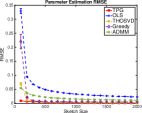
(a) RMSE

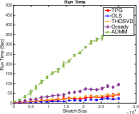
(b) Run Time

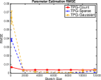
(c) RMSE

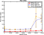
(d) Run Time

Figure 1: Performance comparison on the synthetic dataset over 10 random runs. 1(a) model parameter estimation RMSE for different algorithms, 1(b) running time with respect to sketching size for different algorithms, 1(c) RMSE for different sketching method, 1(d) running time for different sketching method.

We conduct a set of experiments on one synthetic dataset and two real world applications. In this section, we present and analyze the results obtained. We compare TGP with following baseline methods:

• OLS: ordinary least square estimator without low-rank constraint

• THOSVD (De Lathauwer et al., 2000b): a two-step heuristic that first solves the least square and then performs truncated singular value decomposition

• Greedy (Yu et al., 2014): a fast tensor regression solution that sequentially estimates rank one subspace based on Orthogonal Matching Pursuit

• ADMM (Gandy et al., 2011): alternating direction method of multipliers for nuclear norm regularized optimization

7.1 Synthetic Dataset

We construct a model coefficient tensor ${\mathcal{W}}$ of size $30\times 30\times 20$ with Tucker rank equals to $2$ for all modes. Then, we generate the observations ${\mathcal{Y}}$ and ${\mathcal{X}}$ according to multivariate regression model ${\mathcal{Y}}_{:,:,m}={\mathcal{X}}_{:,:,m}{\mathcal{W}}_{:,:,m}+\mathcal{E}_{:,:,m}$ for $m=1,\ldots,M$, where $\mathcal{E}$ is a noise tensor with zero mean Gaussian elements. We generate the time series with $30,000$ time stamps and repeat the procedure for $10$ times.

Figure 1(a) and 1(b) shows the parameter estimation RMSE and the run time error bar with respect to the sketching size. Since the true model is low-rank, simple OLS suffers from poor performance. Other methods are able to converge to the correct solution. The main difference occurs for small sketch size scenario. TPG demonstrates its impressively robustness to noise while others shows high variance in estimation RMSE. ADMM obtains reasonable accuracy and is relatively robust, but is very slow.

We also investigate the impact of sketching scheme on TPG. We compare count sketch (Count) with sketch with i.i.d Gaussian entries (Gaussian) and sparse random projection (Sparse) (Achlioptas, 2003). Figure 1(c) and 1(d) shows the parameter estimation RMSE and the run time errorbar for TPG combined with different random sketching algorithm. TPG with count sketch achieves best performance, especially for small sketch size. The results justify the metrit of leveraging count sketch for noise reduction, in order to accelerate the convergence of TPG algorithm.

7.2 Real Data

In this section, we test the described approaches with two real world application datasets: multi-linear multi-task learning and spatio-temporal forecasting problem.

7.2.1 Multi-linear Multi-task Learning

We compare TPG with state-of-art multi-linear multi-task baseline. Our evaluation follows the same experiment setting in (Romera-Paredes et al., 2013) on the restaurant & consumer dataset, provided by the authors in the paper. The data set contains consumer ratings given to different restaurants. The data has $138$ consumers gave $3$ type of scores for restaurant service. Each restaurant has $45$ attributes for rating prediction. The total number of instances for all the tasks were $3483$. The problem results in a model tensor of dimension $45\times 138\times 3$.

We split the training and testing set with different ratio ranging from 0.1 to 0.9 and randomly select the training data instances. When the training size is small, many tasks contained no training example. We also select 200 instances as the validation set. We compare with MLMTL-C and multi-task feature learning baselines in the original paper. MTL-L21 uses $L_{21}$ regularizer and MTL-Trace is the trace-norm regularized multi-task learning algorithm. The model parameters are selected by minimizing the mean squared error on the validation set.

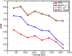
(a) MSE

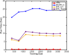
(b) Run Time

Figure 2: Multi-linear multi-task learning performance comparison on the synthetic dataset over 10 random runs. 2(a) average forecasting MSE and 2(b) running time w.r.t. training size.

Figure 2 demonstrates the prediction performance in terms of MSE and runtime with respect to different training size. Compared with MLMTL-C, TPG is around $10\%-25\%$ more accurate and at least $20$ times faster. MTL-L21 or MTL-Trace runs faster than MLMTL-C but also sacrifices accuracy. The difference is more noticeable in the case of small training size. These results are not surprising. Given limited samples and highly correlated tasks in the restaurant score prediction, the model parameters demonstrate low-rank property. In fact, we found that rank $1$ is the optimal setting for this data during the experiments.

7.2.2 Spatio-Temporal Forecasting

For the spatio-temporal forecasting task, we experiment with following two datasets.

Foursquare Check-In

The Foursquare check-in data set contains the users’ check-in records in Pittsburgh area from Feb 24 to May 23, 2012, categorized by different venue types such as Art & Entertainment, College & University, and Food. We extract hourly check-in records of $739$ users in $34$ different venues categories over $3,474$ hours time period as well as users’ friendship network.

USHCN Measurements

The U.S. Historical Climatology Network (USHCN) daily (http://cdiac.ornl.gov/ftp/ushcn_daily/) contains daily measurements for $5$ climate variables for more than $100$ years. The five climate variables correspond to temperature max, temperature min, precipitation, snow fall and snow depth. The records were collected across more than $1,200$ locations and spans over $45,384$ time stamps.

We split the data along the temporal dimension into 80% training set and 20% testing set. We choose VAR (3) model and use 5-fold cross-validation to select the rank during the training phase. For both datasets, we normalize each individual time series by removing the mean and dividing by standard deviation. Due to the memory constraint of the Greedy algorithm, evaluations are conducted on down-sampled datasets.

Table 2: Forecasting RMSE and run time on Foursquare check-in data and USHCN daily measurement for VAR process with 3 lags, trained with 80% of the time series.

	TPG	OLS	THOSVD	Greedy	ADMM
RMSE	0.3580	0.8277	0.4780	0.3639	0.3916
RunTime	37.06	5.85	12.37	290.12	445.41

	TPG	OLS	THOSVD	Greedy	ADMM
RMSE	0.3872	1.4265	0.7224	0.4389	0.5893
RunTime	144.43	23.69	46.26	410.38	6786

Table 2 presents the best forecasting performance (w.r.t sketching size) and the corresponding run time for each of the methods. TPG outperforms baseline methods with higher accuracy. Greedy shows similar accuracy, but TPG converges in very few iterations. For USHCN, TPG achieves much higher accuracy with significantly shorter run time. Those results demonstrate the efficiency of our proposed algorithm for spatio-temporal forecasting tasks.

We further investigate the learned structure of TPG algorithm from USHCN data. Figure 3 shows the spatial-temporal dependency graph on the terrain of California. Each velocity vector represents the aggregated weight learned by TPG from one location to the other. The graph provides an interesting illustration of atmospheric circulation. For example, near Shasta-Trinity National forecast in northern California, the air flow into the forecasts. On the east side along Rocky mountain area, there is a strong atmospheric pressure, leading to wind moving from south east to north west passing the bay area. Another notable atmospheric circulation happens near Salton sea at the border of Utah, caused mainly by the evaporation of the sea.

Figure 3: Velocity vectors plot of spatial-temporal dependency graph obtained via TPG. Results are averaged across all five different climate variables.

8 Discussion

The implication of our approach has several interesting aspects that might shed light upon future algorithmic design.

(1) The projection step in TPG does not depends on data, thus it connects to tensor decomposition techniques such as high order orthogonal iteration (HOOI) (De Lathauwer et al., 2000a). However, there is subtle difference in that the regression would call for early stop of iterative projection as it sequentially search for the orthogonal subspaces.

(2) TPG behaves similarly as first order methods. The convergence rate can be further improved with second order Newton method. This can be done easily by replacing the gradient with Hessian. This modification does not affect the theoretical properties of the proposed algorithm, but would lead to significant empirical improvement (Jain et al., 2010).

9 Conclusion

In this paper, we study tensor regression as a tool to analyze multiway data. We introduce Tensor Projected Gradient to solve the problem. Our approach is built upon projected gradient method, generalizing iterative hard thresholding technique to high order tensors. The algorithm is very simple and general, which can be easily applied to many tensor regression models. It also shares the efficiency of iterative hard thresholding method. We prove that the algorithm converges within a constant number of iterations and the achievable estimation error is linear to the size of the noise. We evaluate our method on multi-linear multi-task learning as well as spatio-temporal forecasting applications. The results show that the our method is significantly faster and is impressively robust to noise.

10 Acknowledgment

This work is supported in part by the U. S. Army Research Office under grant number W911NF-15-1-0491, NSF Research Grant IIS- 1254206 and IIS-1134990. The views and conclusions are those of the authors and should not be interpreted as representing the official policies of the funding agency, or the U.S. Government.

References

- Acar et al. (2007) Acar, Evrim, Aykut-Bingol, Canan, Bingol, Haluk, Bro, Rasmus, and Yener, Bülent. Multiway analysis of epilepsy tensors. Bioinformatics, 23(13):i10–i18, 2007.
- Achlioptas (2003) Achlioptas, Dimitris. Database-friendly random projections: Johnson-lindenstrauss with binary coins. Journal of computer and System Sciences, 66(4):671–687, 2003.
- Blumensath & Davies (2009) Blumensath, Thomas and Davies, Mike E. Iterative hard thresholding for compressed sensing. Applied and Computational Harmonic Analysis, 27(3):265–274, 2009.
- Calamai & Moré (1987) Calamai, Paul H and Moré, Jorge J. Projected gradient methods for linearly constrained problems. Mathematical programming, 39(1):93–116, 1987.
- Candes et al. (2006) Candes, Emmanuel J, Romberg, Justin K, and Tao, Terence. Stable signal recovery from incomplete and inaccurate measurements. Communications on pure and applied mathematics, 59(8):1207–1223, 2006.
- Cichocki et al. (2009) Cichocki, Andrzej, Zdunek, Rafal, Phan, Anh Huy, and Amari, Shun-ichi. Nonnegative matrix and tensor factorizations: applications to exploratory multi-way data analysis and blind source separation. John Wiley & Sons, 2009.
- Clarkson & Woodruff (2013) Clarkson, Kenneth L and Woodruff, David P. Low rank approximation and regression in input sparsity time. In Proceedings of the forty-fifth annual ACM symposium on Theory of computing, pp. 81–90. ACM, 2013.
- Cressie & Wikle (2015) Cressie, Noel and Wikle, Christopher K. Statistics for spatio-temporal data. John Wiley & Sons, 2015.
- De Lathauwer et al. (2000a) De Lathauwer, Lieven, De Moor, Bart, and Vandewalle, Joos. On the best rank-1 and rank-(r 1, r 2,…, rn) approximation of higher-order tensors. SIAM Journal on Matrix Analysis and Applications, 21(4):1324–1342, 2000a.
- De Lathauwer et al. (2000b) De Lathauwer, Lieven, De Moor, Bart, and Vandewalle, Joos. A multilinear singular value decomposition. SIAM journal on Matrix Analysis and Applications, 21(4):1253–1278, 2000b.
- Eckart & Young (1936) Eckart, Carl and Young, Gale. The approximation of one matrix by another of lower rank. Psychometrika, 1(3):211–218, 1936.
- Gandy et al. (2011) Gandy, Silvia, Recht, Benjamin, and Yamada, Isao. Tensor completion and low-n-rank tensor recovery via convex optimization. Inverse Problems, 27(2):025010, 2011.
- Garg & Khandekar (2009) Garg, Rahul and Khandekar, Rohit. Gradient descent with sparsification: an iterative algorithm for sparse recovery with restricted isometry property. In Proceedings of the 26th Annual International Conference on Machine Learning, pp. 337–344. ACM, 2009.
- Hasselmann (1997) Hasselmann, Klaus. Multi-pattern fingerprint method for detection and attribution of climate change. Climate Dynamics, 13(9):601–611, 1997.
- Ishteva et al. (2011a) Ishteva, Mariya, Absil, P-A, Van Huffel, Sabine, and De Lathauwer, Lieven. Best low multilinear rank approximation of higher-order tensors, based on the riemannian trust-region scheme. SIAM Journal on Matrix Analysis and Applications, 32(1):115–135, 2011a.
- Ishteva et al. (2011b) Ishteva, Mariya, Absil, P-A, Van Huffel, Sabine, and De Lathauwer, Lieven. Tucker compression and local optima. Chemometrics and Intelligent Laboratory Systems, 106(1):57–64, 2011b.
- Jain et al. (2010) Jain, Prateek, Meka, Raghu, and Dhillon, Inderjit S. Guaranteed rank minimization via singular value projection. In Advances in Neural Information Processing Systems, pp. 937–945, 2010.
- Kolda & Bader (2009) Kolda, Tamara G and Bader, Brett W. Tensor decompositions and applications. SIAM review, 51(3):455–500, 2009.
- Rauhut et al. (2015) Rauhut, Holger, Schneider, Reinhold, and Stojanac, Željka. Tensor completion in hierarchical tensor representations. In Compressed Sensing and its Applications, pp. 419–450. Springer, 2015.
- Rockafellar (1976) Rockafellar, R Tyrrell. Monotone operators and the proximal point algorithm. SIAM journal on control and optimization, 14(5):877–898, 1976.