Large-strain poroelastic plate theory for polymer gels with applications to swelling-induced morphing of composite plates

Abstract

We derive a large-strain plate model that allows to describe transient, coupled processes involving elasticity and solvent migration, by performing a dimensional reduction of a three-dimensional poroelastic theory. We apply the model to polymer gel plates, for which a specific kinematic constraint and constitutive relations hold. Finally, we assess the accuracy of the plate model with respect to the parent three-dimensional model through two numerical benchmarks, solved by means of the finite element method. Our results show that the theory offers an efficient computational framework for the study of swelling-induced morphing of composite gel plates.

Keywords: plates, large strain, polymer gel, swelling.

1 Introduction

The analysis of plates and shells undergoing large strains has attracted a considerable research effort, especially in computational mechanics (Braun et al., 1994; Sansour, 1995; Basar and Ding, 1996, 1997; Sussman and Bathe, 2013). So far, attention has been essentially restricted to hyperelastic and viscoelastic materials, including rubber-like materials. On the other hand, in the context of thin elastic structures consisting of polymer gels, where rubber-like elasticity is coupled with the motion of a fluid that causes the material to swell, large-strain poroelastic plate models are needed. The complexity of current theories of polymer gel swelling (Hong et al., 2008; Wang and Hong, 2012; Lucantonio et al., 2013) stems from their non-linear, multiphysics and three-dimensional character and typically demands for computationally intensive numerical solutions (Zhang et al., 2009; Bouklas et al., 2015; Chester et al., 2015). In partial response to these issues, the formulation of dimensionally-reduced theories, including poroelastic plate theories, will allow to develop efficient computational models, and occasionally to gain insight from analytical or semi-analytical solutions, which are seldom found for three-dimensional models.

In this spirit but in a different context, a number of plate and shell models has been developed in recent years to describe the mechanics of thin elastic bodies undergoing material growth (Efrati et al., 2009; Dervaux et al., 2009; Lewicka et al., 2010). These models were mainly motivated by the study of shape formation and mechanical instabilities in natural and biological thin structures (Goriely and Ben Amar, 2005). Later, these theories have been applied to model shape morphing of responsive gels (Sharon and Efrati, 2010; Dias et al., 2011) by assimilating swelling to growth. Specifically, in such applications, photolitographic patterning of the cross-linking density of thin gel membranes (Klein et al., 2007; Kim et al., 2012; Wu et al., 2013) and, more generally, fabrication of composite thin gel structures enable three-dimensional transformations through non-homogeneous or anisotropic swelling. Despite their success in reproducing experimental results, these models do not include any thermodynamic treatment of swelling and, as a result, they lack the relation between elasticity of the network and degree of swelling. Such relation is usually introduced phenomenologically through experimental calibration. Finally, all the proposed growth-based models lack an evolution structure, since they do not include the balance of solvent mass, and thus only allow to study the equilibrium shapes of swelling plates (Gemmer and Venkataramani, 2013). Transient swelling processes are fundamental, for instance, in the toughening of homogeneous (Noselli et al., 2016) and composite gels (Lucantonio et al., 2015a; Lucantonio and Noselli, 2016).

Motivated by the observations above, here we introduce a large-strain plate theory for polymer gels obtained by consistent dimensional reduction of the three-dimensional, coupled elasticity-solvent migration model established in Lucantonio et al. (2013). Our theory is not restricted to static equilibrium shapes, but it is also suitable for the study of approach to equilibrium and transient phenomena. This work extends the recent results presented in Lucantonio et al. (2015b), where a membrane theory for swelling polymer gels has been introduced. Our deductive strategy of dimensional reduction employs the weak formulation of the three-dimensional governing equations as a tool to derive the local balance laws for the plate, including the balance of forces, moments and solvent mass. The same deductive approach is employed to obtain the dimensionally reduced counterpart of the three-dimensional swelling constraint, which relates the solvent volume fraction to the volume change of the plate. Thermodynamical consistency is guaranteed through the dissipation inequality, which provides the appropriate constitutive equations for the plate theory, upon introducing for the state variables the same representations along the thickness as those used for the virtual fields. We specialize the constitutive equations for polymer gel plates by employing the Flory-Rehner free energy. In the last section, we study three numerical benchmarks to validate the present plate theory with respect to the parent three-dimensional model. In particular, we show how the proposed plate model can be employed as a computational tool for the shape programming of composite gel plates.

2 Geometry and kinematics of the plate

The ambient space of our theory is represented by the three-dimensional Euclidean point space $\mathcal{E}$, whose associated space of translations is denoted by $\mathcal{V}$. Unless otherwise stated, free Latin indices range over $\{0,1,2\}$, free Greek indices range over $\{1,2\}$, and the standard summation convention over repeated indices is employed. Explicit dependence on time of the fields of interest is omitted.

In its reference configuration, the plate occupies a cylindrical region $\mathcal{B}$ of height $h$ and mid–surface $\mathcal{S}$. For convenience in later computations we parametrize the mid–surface through a generic coordinate system $(s^{1},s^{2})$ ranging in a domain $\mathcal{M}\subset\mathbb{R}^{2}$. Denoting by $\mathring{r}(s)$ the point on $\mathcal{S}$ identified by the coordinates $s=(s^{1},s^{2})$ and letting $\mathring{\mathbf{n}}$ denote the unit vector orthogonal to $\mathcal{S}$, we can write the typical point of the plate as

$$\mathring{p}(s,\zeta)=\mathring{r}(s)+\zeta\mathring{\mathbf{n}}\,,$$ (1)

with $\zeta$ ranging in the interval $(-h/2,+h/2)$. We assume that the function $\mathring{r}:\mathcal{M}\to\mathcal{S}$ is smooth enough so that the forthcoming differential operations performed on $\mathring{r}$ make sense.

Expression (1) provides a parametrization in terms of coordinates $(s^{1},s^{2},\zeta)$ for the reference configuration $\mathcal{B}$ of the plate. The spatial dependence of a (scalar, vectorial, or tensorial) field $f$ defined on $\mathcal{B}$ is expressed using this coordinate system, and we write $f_{,\alpha}=\frac{\partial f}{\partial s^{\alpha}}$ and $f_{,3}=\frac{\partial f}{\partial\zeta}$. In particular, we denote by

$$\mathring{\mathbf{g}}_{\alpha}=\mathring{p}_{,\alpha}=\mathring{r}_{,\alpha},\qquad\mathring{\mathbf{g}}_{3}=\mathring{p}_{,3}=\mathring{\mathbf{n}}$$

the referential covariant basis.

With this notation, we can write the area element of the reference base surface as $\mbox{d}a=\mathring{\Gamma}\,\mbox{d}s^{1}\mbox{d}s^{2}$, with $\mathring{\Gamma}=\mathring{\mathbf{g}}_{1}\times\mathring{\mathbf{g}}_{2}\cdot\mathring{\mathbf{n}}$. Moreover, we denote by $\bm{\nu}(s)$ the outward unit normal to $\partial\mathcal{S}$ at $\mathring{p}(s)$, and by $\ell$ the arc-length parameter of $\partial\mathcal{S}$. Calculus in curvilinear coordinates yields the formulas

$$\nabla f=\operatorname{\nabla_{\!s}}f+f_{,3}\otimes\mathring{\mathbf{n}}\,,\qquad\operatorname{\nabla_{\!s}}f=f_{,\alpha}\otimes\mathring{\mathbf{g}}^{\alpha}\,,$$ (2)

(here, the tensor product between a scalar and a vector is the standard multiplication) where the formulas

$$\mathring{\mathbf{g}}^{1}=\mathring{\Gamma}^{-1}{\mathring{\mathbf{g}}_{2}\times\mathring{\mathbf{n}}}\,,\qquad\mathring{\mathbf{g}}^{2}=\mathring{\Gamma}^{-1}{\mathring{\mathbf{n}}\times\mathring{\mathbf{g}}_{1}}\,,\qquad\mathring{\mathbf{g}}^{3}=\mathring{\mathbf{n}}\,.$$ (3)

express the standard contravariant basis.

The configuration of the plate is described, at each time, by the pair of fields $(p(s,\zeta),c(s,\zeta))$, where $p(s,\zeta)$ is the deformation of the plate and $c(s,\zeta)$ is the solvent concentration per unit reference volume. Plate theories are usually generated by approximating $p(s,\zeta)$ with an expression involving a finite number of fields that depend on $s$ only. The theory we propose in this paper approximates $p(s,\zeta)$ with the expression

$$p(s,\zeta)=r(s)+\zeta\left(1+\frac{{\delta}(s)}{2}\zeta\right)\mathbf{d}(s)$$ (4)

involving three fields: the placement of the mid–surface $r:\mathcal{M}\to\mathcal{E}$, the director $\mathbf{d}:\mathcal{M}\to\mathcal{V}$, and the scalar corrector field $\delta:\mathcal{M}\to\mathbb{R}$. In what follows, we denote by $\mathbf{a}_{\alpha}=r_{,\alpha}$ the covariant basis of the tangent plane to the current configuration of the mid–surface. According to (4) the deformation gradient can be expressed as

$$\mathbf{F}=\nabla p=\mathbf{g}_{\alpha}\otimes\mathring{\mathbf{g}}^{\alpha}+\mathbf{g}_{3}\otimes\mathring{\mathbf{n}}\,,$$ (5)

where

$$\mathbf{g}_{\alpha}=\mathbf{a}_{\alpha}+\zeta\left(1+\frac{\delta}{2}\zeta\right)\mathbf{d}_{,\alpha}+\frac{\delta_{,\alpha}}{2}\mathbf{d}\,,\qquad\mathbf{g}_{3}=\left(1+\zeta\delta\right)\mathbf{d}\,,$$ (6)

is the current covariant basis. The vector $\mathbf{g}_{3}(s,\zeta)$ represents the image under the deformation $p(s,\zeta)$ of an infinitesimal material fiber initially placed at $\mathring{p}(s,\zeta)$ and parallel to $\mathring{\mathbf{n}}$. As is apparent from (6) the fiber becomes parallel to $\mathbf{d}$ and undergoes a non–uniform stretch:

$$\lambda_{3}(s,\zeta)=\sqrt{\mathbf{F}\mathring{\mathbf{n}}\cdot\mathbf{F}\mathring{\mathbf{n}}}=\sqrt{\mathbf{g}_{3}(s,\zeta)\cdot\mathbf{g}_{3}(s,\zeta)}=|(1+\delta(s)\zeta)\mathbf{d}(s)|,$$ (7)

which does not vanish within the interval $[-h/2,h/2]$ provided that $|\delta(s)|<2/h$. The introduction of the scalar field ${\delta}$ in the kinematics of the plate results into a 7-parameter (the other six parameters are the three components of the displacement $\bm{u}(s)=r(s)-\mathring{r}(s)$ of the base surface and the three components of the deformed director $\mathbf{d}(s)$) theory that has been shown to be effective in avoiding locking problems (Braun et al., 1994) in compressible materials, without performing any manipulation of the three-dimensional constitutive equations before dimensional reduction. Typically, in models using a plane-strain (constant thickness) kinematics, locking is avoided by enforcing the plane-stress hypothesis at the three-dimensional level, which is not compatible with plane-strain, but leads nevertheless to a theory that provides accurate results in many cases.

For the sake of calculation, we shall oftentimes find it is convenient to rewrite the deformation as

$$p(s,\zeta)=r(s)+\zeta\mathbf{d}_{1}(s)+\frac{\zeta^{2}}{2}\mathbf{d}_{2}(s)\,,\qquad\mathbf{d}_{1}\equiv\mathbf{d}\,,\qquad\mathbf{d}_{2}\equiv{\delta}\mathbf{d}\,.$$ (8)

Then, letting $\widehat{\mathbf{F}}=\operatorname{\nabla_{\!s}}r=\mathbf{a}_{\alpha}\otimes\mathring{\mathbf{g}}^{\alpha}$, we can rewrite (5) as

$$\mathbf{F}=\left(\widehat{\mathbf{F}}+\zeta\operatorname{\nabla_{\!s}}{\mathbf{d}_{1}}+\frac{\zeta^{2}}{2}\operatorname{\nabla_{\!s}}{\mathbf{d}_{2}}\right)+(\mathbf{d}_{1}+\zeta\mathbf{d}_{2})\otimes\mathring{\mathbf{n}}\,.$$ (9)

As we will see in Section 5, this two-director representation of $\mathbf{F}$ is particularly suitable to express the reduced constitutive equations.

Further, we take the concentration $c$ to be linearly dependent on the thickness coordinate:

$$c(s,\zeta)=c_{0}(s)+\zeta c_{1}(s)\,.$$ (10)

Importantly, we observe that, in principle, neither (4) nor (10) are necessary for the determination of the balance equations of the plate theory from the principle of virtual power, since for that aim only the representations of the virtual fields are involved. Thus, the use of (4), (10) is effectively restricted to performing explicit integrations along the thickness in the derivation of reduced constitutive equations (see Section 5).

3 Balance equations

3.1 Balance of forces and moments

Following Antman (2005); DiCarlo et al. (2001), we derive the balance of forces and moments for the plate-like body $\mathcal{B}$ starting from the principle of virtual power

$$\mathcal{I}^{h}_{\rm m}(\mathcal{M},\widetilde{\mathbf{v}})=\mathcal{W}^{h}_{\rm m}(\mathcal{M},\widetilde{\mathbf{v}})\,,$$ (11)

which states the equality between the virtual expenditures of internal mechanical power

$$\mathcal{I}^{h}_{\rm m}(\mathcal{M},\widetilde{\mathbf{v}})=\int_{\mathcal{M}}\int_{-h/2}^{h/2}{\mathbf{S}\cdot\nabla\widetilde{\mathbf{v}}\,\mbox{d}\zeta\mbox{d}a}$$ (12)

and external mechanical power

$$\mathcal{W}^{h}_{\rm m}(\mathcal{M},\widetilde{\mathbf{v}})=\int_{\mathcal{M}}\int_{-h/2}^{h/2}{\mathbf{f}\cdot\widetilde{\mathbf{v}}}\,\mbox{d}\zeta\mbox{d}a+\int_{\mathcal{M}}\left(\mathbf{t}\cdot\widetilde{\mathbf{v}}\right)\Big{|}_{\pm h/2}\,\mbox{d}a+\int_{\partial\mathcal{M}}\int_{-h/2}^{h/2}{\mathbf{t}\cdot\widetilde{\mathbf{v}}}\,\mbox{d}\ell\,,$$ (13)

for any virtual velocity field $\widetilde{\mathbf{v}}$. Here, $\mathbf{S}$ is the Piola-Kirchhoff stress and the system of external forces is represented by the body force $\mathbf{f}$ acting on $\mathcal{B}$ and the surface traction $\mathbf{t}$ acting on $\partial\mathcal{B}$. The crucial point when using (11) is to restrict test velocities to those compatible with the kinematic constraint that generates the theory. Here, consistent with the expression (8) of the deformation of the plate, we assume that, for $s$ fixed, the virtual velocity field is a quadratic polynomial of $\zeta$:

$$\widetilde{\mathbf{v}}(s,\zeta)=\widetilde{\mathbf{v}}_{0}(s)+\zeta{\widetilde{\mathbf{v}}}_{1}(s)+\frac{\zeta^{2}}{2}{\widetilde{\mathbf{v}}}_{2}(s)\,,$$ (14)

so that the internal virtual power expended is

$$\begin{split}\int_{\mathcal{M}}\int_{-h/2}^{h/2}{\left[\bm{S}\cdot\left(\operatorname{\nabla_{\!s}}{\widetilde{\mathbf{v}}_{0}}+\zeta\operatorname{\nabla_{\!s}}{{\widetilde{\mathbf{v}}}_{1}}+\frac{\zeta^{2}}{2}\operatorname{\nabla_{\!s}}{{\widetilde{\mathbf{v}}}_{2}}\right)+\bm{s}\cdot({\widetilde{\mathbf{v}}}_{1}+\zeta{\widetilde{\mathbf{v}}}_{2})\right]\,\mbox{d}\zeta\mbox{d}a}\,,\end{split}$$ (15)

where $\bm{S}=\mathbf{S}\mathring{\mathbf{P}}$, $\bm{s}=\mathbf{S}\mathring{\mathbf{n}}$ with $\mathring{\mathbf{P}}=\mathring{\mathbf{g}}_{\alpha}\otimes\mathring{\mathbf{g}}^{\alpha}$ the in-plane projector. Introducing the stress resultants

$$\bm{S}^{(i)}(s)=\int_{-h/2}^{h/2}\frac{\zeta^{i}}{i!}\bm{S}(s,\zeta)\,\mbox{d}\zeta\,, \bm{s}^{(i)}(s)=\int_{-h/2}^{h/2}\frac{\zeta^{(i)}}{i!}{\mathbf{s}}(s,\zeta)\,\mbox{d}\zeta\,,$$ (16)

we can recast (15) as

$${\mathcal{I}}_{\rm m}(\mathcal{M},\widetilde{\mathbf{v}}_{i})=\int_{\mathcal{M}}\left(\bm{S}^{(i)}\cdot\operatorname{\nabla_{\!s}}\widetilde{\mathbf{v}}_{i}+{{\bm{s}}}^{(0)}\cdot\widetilde{\mathbf{v}}_{1}+{{\bm{s}}}^{(1)}\cdot\widetilde{\mathbf{v}}_{2}\right)\mbox{d}a\,.$$ (17)

Likewise, introducing the bulk force resultants

$$\mathbf{f}^{(i)}(s)=\int_{-h/2}^{h/2}{\frac{\zeta^{(i)}}{i!}\mathbf{f}(s,\zeta)\,\mbox{d}\zeta}+\left(\frac{\zeta^{(i)}}{i!}\mathbf{t}(s,\zeta)\right)\Big{|}_{\zeta=-h/2}+\left(\frac{\zeta^{(i)}}{i!}\mathbf{t}(s,\zeta)\right)\Big{|}_{\zeta=h/2}$$ (18)

defined for $s\in\mathcal{M}$, and the boundary force resultants

$$\mathbf{t}^{(i)}(s)=\int_{-h/2}^{h/2}{\frac{\zeta^{(i)}}{i!}\mathbf{t}(s,\zeta)\,\mbox{d}\zeta}$$ (19)

defined for $s\in\partial\mathcal{M}$, we can write the external power as

$${\mathcal{W}}_{\rm m}(\mathcal{M},\widetilde{\mathbf{v}}_{i})=\int_{\mathcal{M}}\left(\mathbf{f}^{(i)}\cdot\widetilde{\mathbf{v}}_{i}\right)\mbox{d}a+\int_{\partial\mathcal{M}}\left(\mathbf{t}^{(i)}\cdot\widetilde{\mathbf{v}}_{i}\right)\mbox{d}\ell\,.$$ (20)

When deriving balance equations in strong form by exploiting the arbitrariness of the virtual fields, some care is required, because the virtual velocities $\widetilde{\mathbf{v}}_{1}$ and $\widetilde{\mathbf{v}}_{2}$ are not independent. Indeed, it holds $\widetilde{\mathbf{v}}_{2}=\widetilde{\delta}\mathbf{d}+{\delta}\widetilde{\mathbf{v}}_{1}$, since $\mathbf{d}_{2}={\delta}\mathbf{d}$. Substitution of this relation into the virtual–power functionals (17) and (20), yields, for the internal power

$${\mathcal{I}}^{\prime}_{\rm m}(\mathcal{M},\widetilde{\mathbf{v}}_{0},\widetilde{\mathbf{v}}_{1},\widetilde{\delta})=\int_{\mathcal{M}}\left(\mathbf{N}\cdot\operatorname{\nabla_{\!s}}\widetilde{\mathbf{v}}_{0}+\mathbf{M}\cdot\operatorname{\nabla_{\!s}}\widetilde{\mathbf{v}}_{1}+\mathbf{q}\cdot\widetilde{\mathbf{v}}_{1}+\bm{\tau}\cdot\operatorname{\nabla_{\!s}}\widetilde{\delta}+\tau\widetilde{\delta}\right)\mbox{d}a\,,$$ (21)

where

$$\mathbf{N}=\bm{S}^{(0)}\,, \mathbf{M}=\bm{S}^{(1)}+{\delta}{\bm{S}}^{(2)}\,, \mathbf{q}={{\bm{s}}}^{(0)}+{\delta}{\bm{s}}^{(1)}+\bm{S}^{(2)}\operatorname{\nabla_{\!s}}{\delta}\,,$$ (22)

$${\bm{\tau}}={{\bm{S}}^{(2)}}^{\rm T}{\mathbf{d}}\,, \tau={\bm{s}}^{(1)}\cdot\mathbf{d}+\bm{S}^{(2)}\cdot\operatorname{\nabla_{\!s}}\mathbf{d}\,,$$

and, for the external power

$${\mathcal{W}}^{\prime}_{\rm m}(\mathcal{M},\widetilde{\mathbf{v}}_{0},\widetilde{\mathbf{v}}_{1},\widetilde{\delta})=\int_{\mathcal{M}}\left(\mathbf{f}^{(0)}\cdot\widetilde{\mathbf{v}}_{0}+\overline{\mathbf{f}}^{(1)}\cdot\widetilde{\mathbf{v}}_{1}+f_{d}^{(2)}\widetilde{\delta}\right)\mbox{d}a+\int_{\partial\mathcal{M}}\left(\mathbf{t}^{(0)}\cdot\widetilde{\mathbf{v}}_{0}+\overline{\mathbf{t}}^{(1)}\cdot\widetilde{\mathbf{v}}_{1}+t^{(2)}_{d}\widetilde{\delta}\right)\mbox{d}\ell\,,$$ (23)

where

$$\overline{\mathbf{f}}^{(1)}=\mathbf{f}^{(1)}+{\delta}\mathbf{f}^{(2)}\,, f_{d}^{(2)}=\mathbf{f}^{(2)}\cdot\mathbf{d}\,, \overline{\mathbf{t}}^{(1)}=\mathbf{t}^{(1)}+{\delta}\mathbf{t}^{(2)}\,, t_{d}^{(2)}=\mathbf{t}^{(2)}\cdot\mathbf{d}\,.$$ (24)

For simplicity, we assume that the boundary $\partial\mathcal{M}$ is partitioned into disjoint parts $\partial_{\rm m}^{0}\mathcal{M}$ and $\partial_{\rm m}^{1}\mathcal{M}$, with natural (essential) boundary conditions being prescribed on the former (latter). Then, from the arbitrariness of $(\widetilde{\mathbf{v}}_{0},\widetilde{\mathbf{v}}_{1},\widetilde{\delta})$ in the virtual–power balance

$$\mathcal{I}^{\prime}_{\rm m}(\mathcal{M},\widetilde{\mathbf{v}}_{0},\widetilde{\mathbf{v}}_{1},\widetilde{\delta})=\mathcal{W}^{\prime}_{\rm c}(\mathcal{M},\widetilde{\mathbf{v}}_{0},\widetilde{\mathbf{v}}_{1},\widetilde{\delta})$$ (25)

we deduce the balance equations and the corresponding natural boundary conditions, namely,

$$\operatorname{\mbox{div}_{s}}\mathbf{N}+\mathbf{f}^{(0)}=\mathbf{0}\,, \mbox{in}\ \mathcal{M}\,,$$ (26a)

$$\operatorname{\mbox{div}_{s}}\mathbf{M}-\mathbf{q}+\overline{\mathbf{f}}^{(1)}=\mathbf{0}\,, \mbox{in}\ \mathcal{M}\,,$$ (26b)

$$\operatorname{\mbox{div}_{s}}\bm{\tau}-\tau+f_{d}^{(2)}=0\,, \mbox{in}\ \mathcal{M}\,,$$ (26c)

and

$$\mathbf{N}\bm{\nu}=\mathbf{t}^{(0)}\,, \mbox{on}\ \partial^{0}_{\rm m}\mathcal{M}\,,$$ (27a)

$$\mathbf{M}\bm{\nu}=\overline{\mathbf{t}}^{(1)}\,, \mbox{on}\ \partial^{0}_{\rm m}\mathcal{M}\,,$$ (27b)

$$\bm{\tau}\cdot\bm{\nu}=t_{d}^{(2)}\,, \mbox{on}\ \partial^{0}_{\rm m}\mathcal{M}\,.$$ (27c)

It is easily checked that the symmetry condition $\mathbf{S}\mathbf{F}^{\rm T}\in{\rm Sym}$ entails

$$\mathbf{N}\widehat{\mathbf{F}}^{\rm T}+\mathbf{M}\operatorname{\nabla_{\!s}}\mathbf{d}^{\rm T}+\mathbf{q}\otimes\mathbf{d}\in\mbox{Sym}.$$ (28)

The tensorial identity (28) is equivalent to

$$\mathbf{n}^{\alpha}\times\mathbf{a}_{\alpha}+\mathbf{m}^{\alpha}\times\mathbf{d}_{,\alpha}+\mathbf{q}\times\mathbf{d}=\mathbf{0}\,,$$ (29)

where $\mathbf{n}^{\alpha}=\mathbf{N}\mathring{\mathbf{g}}^{\alpha}$ and $\mathbf{m}^{\alpha}=\mathbf{M}\mathring{\mathbf{g}}^{\alpha}$. This relation can also be obtained by imposing invariance of the internal power expended within every part of the plate under superposed rigid velocity fields. In view of (29), by taking the cross and scalar products of (26b) with $\mathbf{d}$ we obtain, respectively,

$$\operatorname{\mbox{div}_{s}}(\mathbf{D}\mathbf{M})-\mathbf{n}^{\alpha}\times\mathbf{a}_{\alpha}+{\mathbf{d}}\times\overline{\mathbf{f}}^{(1)}=\mathbf{0}\,,$$ (30a)

$$\operatorname{\mbox{div}_{s}}(\mathbf{M}^{\rm T}\mathbf{d})-\mathbf{M}\cdot\operatorname{\nabla_{\!s}}\mathbf{d}-\mathbf{d}\cdot\mathbf{q}+\mathbf{d}\cdot\overline{\mathbf{f}}^{(1)}=0\,,$$ (30b)

where $\mathbf{D}$ is the skew tensor associated to $\mathbf{d}$. From (30), we can recover the classical forms of the balances of torques and director forces for a 6-parameter plate by setting ${\delta}=0$, see Antman (2005); DiCarlo et al. (2001). For a 7-parameter plate, these equations are supplemented by the second-order balance of director forces (26c).

3.2 Balance of solvent mass

In the applications consider here, a flux of solvent is prescribed over the lateral surface of the plate, including the top and bottom faces. The strong form of the balance of solvent mass reads

$$\dot{c}+\operatorname{\mbox{div}}\mathbf{h}=0\,, \mbox{in }\mathcal{B}\,,$$ (31a)

$$-\mathbf{h}\cdot\bm{\nu}=\beta\,, \mbox{on }\partial\mathcal{M}\times(-h/2,+h/2)\,,$$ (31b)

where $\mathbf{h}$ is the referential solvent flux, and $\beta$ is a surface supply of solvent.

With a view towards obtaining a reduced theory, we replace the pointwise statements (31) with their weak form. Inspired by Duda et al. (2010), we interpret such weak form as a version of the virtual-power principle whereby chemical potential is a test field that enters along with its gradient in the power expenditure. Specifically, we prescribe the following representations for virtual expenditures of internal chemical power

$$\mathcal{I}^{h}_{\rm c}(\mathcal{M},\widetilde{\mu})=\int_{\mathcal{M}}\int_{-h/2}^{h/2}(\dot{c}\widetilde{\mu}-\mathbf{h}\cdot\nabla\widetilde{\mu})\,\mbox{d}\zeta\mbox{d}a\,,$$ (32)

and external chemical power

$$\mathcal{W}^{h}_{\rm c}(\mathcal{M},\widetilde{\mu})=\int_{\partial\mathcal{M}}\int_{-h/2}^{h/2}\beta\widetilde{\mu}\,\mbox{d}\zeta\mbox{d}\ell+\int_{\mathcal{M}\times\left\{+\frac{h}{2},-\frac{h}{2}\right\}}\beta\widetilde{\mu}\,\mbox{d}a\,.$$ (33)

Then, the three-dimensional pointwise balance equations (31) are recovered on imposing that the external and internal chemical powers be balanced

$$\mathcal{I}^{h}_{\rm c}(\mathcal{M},\widetilde{\mu})=\mathcal{W}^{h}_{\rm c}(\mathcal{M},\widetilde{\mu})$$ (34)

for any virtual chemical potential $\widetilde{\mu}$.

To arrive at a system of reduced equations, we enforce the principle of virtual power (34) on the class of virtual chemical potentials that depend linearly on $\zeta$:

$$\widetilde{\mu}(s,\zeta)=\widetilde{\mu}_{0}(s)+\zeta\widetilde{\mu}_{1}(s)\,,$$ (35)

consistent with the representation (10) for the work-conjugate field $c$. Granted (35) and using (2) with $\phi=\widetilde{\mu}$, we can write the internal chemical power as:

$$\mathcal{I}_{c}(\mathcal{M},\widetilde{\mu}_{0},\widetilde{\mu}_{1})=\int_{\mathcal{M}}\left(\dot{c}^{(0)}\widetilde{\mu}_{0}+\dot{c}^{(1)}\widetilde{\mu}_{1}-\bm{h}^{(0)}\cdot\operatorname{\nabla_{\!s}}{\widetilde{\mu}_{0}}-h_{3}^{(0)}\widetilde{\mu}_{1}-\bm{h}^{(1)}\cdot\operatorname{\nabla_{\!s}}{\widetilde{\mu}_{1}}\right)\mbox{d}a\,,$$ (36)

where we have introduced the moments of the concentration

$$c^{(i)}(s)=\int_{-h/2}^{h/2}\frac{\zeta^{i}}{i!}c(s,\zeta)\,\mbox{d}\zeta\,,$$ (37)

and of the solvent flux

$$\bm{h}^{(i)}(s)=\int_{-h/2}^{h/2}\frac{\zeta^{i}}{i!}\bm{h}(s,\zeta)\,\mbox{d}\zeta\,,\quad\bm{h}=\mathring{\mathbf{P}}\mathbf{h}\,,$$ (38a)

$$h_{3}^{(i)}(s)=\int_{-h/2}^{h/2}\frac{\zeta^{i}}{i!}h_{3}(s,\zeta)\,\mbox{d}\zeta\,,\quad h_{3}=\mathbf{h}\cdot\mathring{\mathbf{a}}_{3}\,.$$ (38b)

Likewise, the external power becomes

$$\mathcal{W}_{\rm c}(\mathcal{M},\widetilde{\mu}_{0},\widetilde{\mu}_{1})=\int_{\partial\mathcal{M}}(\beta^{(0)}\widetilde{\mu}_{0}+\beta^{(1)}\widetilde{\mu}_{1})\mbox{d}\ell+\int_{\mathcal{M}}(\overline{\beta}^{(0)}\widetilde{\mu}_{0}+\overline{\beta}^{(1)}\widetilde{\mu}_{1})\,\mbox{d}a\,.$$ (39)

where

$$\beta^{(i)}(s) =\int_{-h/2}^{h/2}\frac{\zeta^{i}}{i!}\beta(s,\zeta)\,\mbox{d}\zeta\,,\qquad s\in\partial\mathcal{M}\,,$$ (40a)

$$\overline{\beta}^{(i)}(s) =\sum_{\zeta=\pm\frac{h}{2}}\frac{\zeta^{i}}{i!}\beta(s,\zeta)\,\mbox{d}\zeta\,,\qquad s\in\mathcal{M}.$$ (40b)

With these definitions the principle of virtual power (34) may be written as

$$\mathcal{I}_{\rm c}(\mathcal{M},\widetilde{\mu}_{0},\widetilde{\mu}_{1})=\mathcal{W}_{\rm c}(\mathcal{M},\widetilde{\mu}_{0},\widetilde{\mu}_{1})$$ (41)

for any $\widetilde{\mu}_{0}$ and $\widetilde{\mu}_{1}$.

We partition the boundary of $\mathcal{M}$ into parts $\partial_{\rm c}^{0}\mathcal{M}$ and $\partial_{\rm c}^{1}\mathcal{M}$, and we impose essential boundary conditions for the chemical potential on $\partial_{\rm c}^{1}\mathcal{M}$. On exploiting the arbitrariness of the virtual chemical potential, i.e. of the fields $\widetilde{\mu}_{0}$ and $\widetilde{\mu}_{1}$, in $\mathcal{M}\cup\partial_{\rm c}^{0}\mathcal{M}$, we obtain the balance equations

$$\dot{c}^{(0)}+\operatorname{\mbox{div}_{s}}{\bm{h}^{(0)}}=\overline{\beta}^{(0)}\,, \mbox{in}\ \mathcal{M}\,,$$ (42a)

$$\dot{c}^{(1)}+\operatorname{\mbox{div}_{s}}{\bm{h}^{(1)}}-h_{3}^{(0)}=\overline{\beta}^{(1)}\,, \mbox{in}\ \mathcal{M}\,,$$ (42b)

and the natural boundary conditions

$$-\bm{h}^{(0)}\cdot\bm{\nu}=\beta^{(0)}\,, \mbox{on}\ \partial_{\rm c}^{0}\mathcal{M}\,,$$ (43a)

$$-\bm{h}^{(1)}\cdot\bm{\nu}=\beta^{(1)}\,, \mbox{on}\ \partial_{\rm c}^{0}\mathcal{M}\,.$$ (43b)

Notice that the above equations do not give explicitly the concentration field. However, if we assume that the concentration field has the representation (10), then we can obtain from (42) a set of evolution equations for $c_{0}$ and $c_{1}$. To this aim, it suffices to make use of the following identities:

$$c^{(0)}=hc_{0}\,,\qquad c^{(1)}=\frac{h^{3}}{12}c_{1}\,.$$ (44a)

Then, the balance equations (42) become

$$h\dot{c}_{0}+\operatorname{\mbox{div}_{s}}{\bm{h}^{(0)}}=\overline{\beta}^{(0)}\,, \mbox{in}\ \mathcal{M}\,,$$ (45a)

$$\frac{h^{3}}{12}\dot{c}_{1}+\operatorname{\mbox{div}_{s}}{\bm{h}^{(1)}}-h_{3}^{(0)}=\overline{\beta}^{(1)}\,, \mbox{in}\ \mathcal{M}\,.$$ (45b)

Remark: essential boundary conditions for chemical potential. In the considerations leading to (45), essential boundary conditions for chemical potential have been imposed only on the lateral mantle $\partial\mathcal{M}\times\left(-\frac{h}{2},+\frac{h}{2}\right)$ of the plate. This restriction can be easily removed, and one can impose essential conditions on parts of the top and bottom face of the plate, to be handled by making use of Lagrange multipliers. To be specific: let the boundary values of the chemical potential field be assigned values $\mu^{-}$ and $\mu^{+}$ on parts of the top and bottom faces, which we denote by $\mathcal{M}^{+}\times\left\{\frac{h}{2}\right\}$ and $\mathcal{M}^{-}\times\left\{\frac{h}{2}\right\}$, with $\mathcal{M}^{+}\subseteq\mathcal{M}$ and $\mathcal{M}^{-}\subseteq\mathcal{M}$. Then, denoting by $\chi^{+}:\mathcal{M}\to\{0,1\}$ and $\chi^{-}:\mathcal{M}\to\{0,1\}$ the characteristic functions of $\mathcal{M}^{+}$ and $\mathcal{M}^{-}$, respectively, we add the following reactive term

$$\mathcal{W}_{\rm c}^{r}(\mathcal{M},\widetilde{\mu}_{0},\widetilde{\mu}_{1})=\int_{\mathcal{M}}\Big{(}\chi^{+}r^{+}\big{(}\widetilde{\mu}_{0}+\frac{h}{2}\widetilde{\mu}_{1}\big{)}+\chi^{-}r^{-}\big{(}\widetilde{\mu}_{0}+\frac{h}{2}\widetilde{\mu}_{1}\big{)}\Big{)}\,\mbox{d}a$$

to the external power (39). Then, the additional reactive contributions $\chi^{+}r^{+}+\chi^{-}r^{-}$ and $\frac{h}{2}(\chi^{+}r^{+}-\chi^{-}r^{-})$ appear on the right–hand sides of the first and second equation in (45), respectively.

4 Swelling constraint

For a poroelastic medium undergoing large strain, the assumption of incompressibility of both the solid and the solvent implies that the deformation gradient $\mathbf{F}$ and the concentration $c$ obey the incompressibility constraint (Hong et al., 2008; Lucantonio et al., 2013)

$$J=\det\mathbf{F}=1+\Omega(c-c_{\star})\,,$$ (46)

where $c_{\star}$ is the homogeneous solvent concentration in the reference state. Since the deformation is a polynomial of degree 2 with respect to $\zeta$, its determinant is a polynomial of degree 6 with respect to the same variable. Now, recalling from (10) that concentration is a first–order polynomial in $\zeta$, the constraint (46) cannot be satisfied pointwise.

This state of matters leads us to relax constraint (46), by replacing it with a weak constraint

$$\int_{\mathcal{M}}\int_{-h/2}^{h/2}{[J-1-\Omega(c-c_{\star})]\tilde{p}\,\mbox{d}\zeta\mbox{d}a}=0\,,$$ (47)

where the virtual pressure $\tilde{p}$ has the representation $\tilde{p}(s,\zeta)=\tilde{p}_{0}(s)+\zeta\tilde{p}_{1}(s)$. By enforcing the weak form of the incompressibility constraint with degree-1 virtual pressures we are going to deduce, for each point $s$ of the base surface, a set of two equations relating the deformation with the fields $c_{0}$ and $c_{1}$.

From the identity $J=(\mathbf{F}\mathring{\mathbf{g}}_{1}\times\mathbf{F}\mathring{\mathbf{g}}_{2}\cdot\mathbf{F}\mathring{\mathbf{n}})/(\mathring{\mathbf{g}}_{1}\times\mathring{\mathbf{g}}_{2}\cdot\mathring{\mathbf{n}})$ and from (5) we find $J={\mathbf{g}}_{1}\times{\mathbf{g}}_{2}\cdot{\mathbf{g}}_{3}/\mathring{\Gamma}$. Thus, using (6) we compute:

$$\begin{split}J&=\left(\mathbf{r}_{0}+\zeta\mathbf{r}_{1}+\frac{\zeta^{2}}{2}\mathbf{r}_{2}\right)\cdot(1+\zeta\delta)\mathbf{d}+o(\zeta^{2})\,,\end{split}$$ (48)

with

$$\mathbf{r}_{0}=\frac{\mathbf{a}_{1}\times\mathbf{a}_{2}}{\mathring{\Gamma}}\,,\qquad\mathbf{r}_{1}=\frac{\mathbf{d}_{,1}\times\mathbf{a}_{2}-\mathbf{d}_{,2}\times\mathbf{a}_{1}}{\mathring{\Gamma}}\,,\qquad\mathbf{r}_{2}=\delta\mathbf{r}_{1}+\frac{(\delta_{,2}\mathbf{a}_{1}-\delta_{,1}\mathbf{a}_{2})\times\mathbf{d}+2\mathbf{d}_{,1}\times\mathbf{d}_{,2}}{\mathring{\Gamma}}\,.$$ (49)

Then, we rely on the arbitrariness of $\tilde{p}_{0}(s)$ and $\tilde{p}_{1}(s)$ to obtain the pair of equations holding pointwise in $\mathcal{M}$:

$$1+\Omega(c_{0}-c_{\star}) =\mathbf{r}_{0}\cdot\mathbf{d}+\frac{h^{2}}{24}(2\delta\mathbf{r}_{1}+\mathbf{r}_{2})\cdot\mathbf{d}\,,$$ (50a)

$$\Omega c_{1} =\frac{h^{3}}{12}(\delta\mathbf{r}_{0}+\mathbf{r}_{1})\cdot\mathbf{d}\,.$$ (50b)

5 Thermodynamics and constitutive equations

In this section we obtain constitutive equations for the stress resultants and the flux resultants, starting from those that govern the large-strain behavior of three dimensional poroelastic bodies with incompressible constituents. We first deduce general relations; then, we consider the specialization of these relations to composite polymer gel plates.

5.1 General relations

We begin by assuming that the free energy per unit referential volume obeys the constitutive equation

$$\psi=\widehat{\psi}(\mathbf{F},c).$$ (51)

For $\mathcal{P}\subset\mathcal{M}$ we write the dissipation inequality as

$$\begin{split}&\int_{\mathcal{P}}\int_{-h/2}^{h/2}{\left[\dot{\psi}-p\left(\mathbf{F}^{\star}\cdot\dot{\mathbf{F}}-\Omega\dot{c}\right)\right]\mbox{d}\zeta\mbox{d}a}\leq\mathcal{I}^{h}_{\rm m}(\mathcal{P},\mathbf{v})+\mathcal{I}^{h}_{\rm c}(\mathcal{P},\mu),\end{split}$$ (52)

where $\mathcal{I}^{h}_{\rm m}(\mathcal{P},\mathbf{v})$ and $\mathcal{I}^{h}_{\rm c}(\mathcal{P},\mu)$ are, respectively, the mechanical and the chemical powers given in (12) and (32) expended within a part $\mathcal{P}\times(-h/2,+h/2)$ on the actual velocity $\mathbf{v}=\dot{p}$ and chemical potential. Here, $\mathbf{F}^{\star}$ is the cofactor of $\mathbf{F}$:

$$\mathbf{F}^{\star}=J\mathbf{g}^{i}\otimes\mathring{\mathbf{g}}_{i},$$ (53)

where

$$\mathbf{g}^{1}=\frac{\mathbf{g}_{2}\times\mathbf{g}_{3}}{\Gamma}\,,\qquad\mathbf{g}^{2}=\frac{\mathbf{g}_{3}\times\mathbf{g}_{1}}{\Gamma}\,,\qquad\mathbf{g}^{3}=\frac{\mathbf{g}_{1}\times\mathbf{g}_{2}}{\Gamma}\,,\qquad\mbox{with}\qquad\Gamma=\mathbf{g}_{1}\times\mathbf{g}_{2}\cdot\mathbf{g}_{3}$$ (54)

are the contravariant basis vectors in the current configuration.

We consider evolution processes such that the deformation and the concentration obey the restrictions (4) and (10). For any such process, the velocity and the swelling rate (the time derivative of the concentration) have the form

$$\mathbf{v}(s,\zeta)=\mathbf{v}_{0}(s)+\zeta\mathbf{v}_{1}(s)+\frac{\zeta^{2}}{2}\mathbf{v}_{2}(s)\qquad\mbox{and}\qquad\dot{c}(s,\zeta)=\dot{c}_{0}(s)+\zeta\dot{c}_{1}(s).$$ (55)

From (55) and from the constitutive equation (51) we obtain

$$\int_{-h/2}^{h/2}\dot{\psi}\,\mbox{d}\zeta\mbox{d}a=(\partial_{\mathbf{F}}\widehat{\psi})^{(i)}\cdot\operatorname{\nabla_{\!s}}\mathbf{v}_{i}+(\partial_{\mathbf{F}}\widehat{\psi})^{(0)}[\mathring{\mathbf{n}}]\cdot\mathbf{v}_{1}+(\partial_{\mathbf{F}}\widehat{\psi})^{(1)}[\mathring{\mathbf{n}}]\cdot\mathbf{v}_{2}+(\partial_{c}\widehat{\psi})^{(0)}\dot{c}_{0}+(\partial_{c}\widehat{\psi})^{(1)}\dot{c}_{1},$$ (56)

where

$$(\partial_{\mathbf{F}}\widehat{\psi})^{(i)}=\left(\int_{-h/2}^{h/2}\frac{\zeta^{i}}{i!}\partial_{\mathbf{F}}\widehat{\psi}(\mathbf{F},c)\,\mbox{d}\zeta\right)\mathring{\mathbf{P}}\qquad\textrm{and}\qquad(\partial_{c}\widehat{\psi})^{(i)}=\int_{-h/2}^{h/2}\frac{\zeta^{i}}{i!}\partial_{c}\widehat{\psi}(\mathbf{F},c)\,\mbox{d}\zeta.$$ (57)

Thanks to the identity (53), we have the following representation for the pressure power:

$$\begin{split}\int_{-h/2}^{h/2}{p\mathbf{F}^{\star}\cdot\dot{\mathbf{F}}\,\mbox{d}\zeta}&=\bm{S}_{p}^{(i)}\cdot\operatorname{\nabla_{\!s}}{\mathbf{v}}_{i}+{{\bm{s}}}_{p}^{(\rm 0)}\cdot{\mathbf{v}}_{1}+{{\bm{s}}}_{p}^{(1)}\cdot{\mathbf{v}}_{2},\end{split}$$ (58)

where

$$\bm{S}_{p}^{(i)}=\left(\int_{-h/2}^{h/2}{\frac{\zeta^{i}}{i!}pJ\mathbf{g}^{\alpha}\,\mbox{d}\zeta}\right)\otimes\mathring{\mathbf{g}}_{\alpha}\qquad\textrm{and}\qquad\mathbf{s}_{p}^{(i)}=\int_{-h/2}^{h/2}\frac{\zeta^{i}}{i!}pJ\mathbf{g}^{3}\,\mbox{d}\zeta.$$ (59)

Finally, consistent with the representation of the virtual chemical potential we have selected in (35) to enforce mass balance, we assume that the chemical potential has the form

$$\mu(s,\zeta)=\mu_{0}(s)+\zeta\mu_{1}(s)\,.$$ (60)

Then, with calculations analogous to those leading to (17) and (36), the internal powers in (52) may be recast as $\mathcal{I}_{\rm m}(\mathcal{P},\mathbf{v}_{i})$ and $\mathcal{I}_{\rm c}(\mathcal{P},\mu_{0},\mu_{1})$, respectively, where the virtual fields in (17) and (36) are replaced by the actual fields $\mathbf{v}_{i}$ and $\mu_{i}$.

On account of the reduced representations of the internal powers and the expressions (56) and (58) for the time rate of the free energy and the reactive power, the dissipation inequality (52) reads

$$\begin{split}&\int_{\mathcal{P}}\left[\left((\partial_{\mathbf{F}}\widehat{\psi})^{(i)}+\bm{S}^{(i)}_{p}\right)\cdot\operatorname{\nabla_{\!s}}\mathbf{v}_{i}+\left((\partial_{\mathbf{F}}\widehat{\psi})^{(0)}[\mathring{\mathbf{n}}]-\bm{s}^{(0)}_{p}\right)\cdot\mathbf{v}_{1}+\left((\partial_{\mathbf{F}}\widehat{\psi})^{(1)}[\mathring{\mathbf{n}}]-\bm{s}^{(1)}_{p}\right)\cdot\mathbf{v}_{2}\right]\mbox{d}a\\ &\quad+\int_{\mathcal{P}}\left[\left((\partial_{c}\widehat{\psi})^{(0)}-p^{(0)}\right)\dot{c}_{0}+\left((\partial_{c}\widehat{\psi})^{(1)}-p^{(1)}\right)\dot{c}_{1}\right]\mbox{d}a\\ &\leq\quad\int_{\mathcal{P}}\left(\bm{S}^{(i)}\cdot\operatorname{\nabla_{\!s}}{\mathbf{v}}_{i}+{{\bm{s}}}^{(0)}\cdot{\mathbf{v}}_{1}+{{\bm{s}}}^{(1)}\cdot{\mathbf{v}}_{2}\right)\mbox{d}a\\ &\quad+\int_{\mathcal{P}}\left(\mu^{(0)}\dot{c}_{0}+\mu^{(1)}\dot{c}_{1}-\bm{h}^{(0)}\cdot\operatorname{\nabla_{\!s}}\mu_{0}-h_{3}^{(0)}{\mu}_{1}-\bm{h}^{(1)}\cdot\operatorname{\nabla_{\!s}}{{\mu}_{1}}\right)\mbox{d}a.\end{split}$$ (61)

Consistent with the requirement that (61) holds for every choice of the velocities (55) we prescribe

$$\bm{S}^{(i)}=(\partial_{\mathbf{F}}\widehat{\psi})^{(i)}-\bm{S}^{(i)}_{p}\,, i=0,1,2,$$ (62a)

$$\bm{s}^{(i)}=(\partial_{\mathbf{F}}\widehat{\psi})^{({i})}[\mathring{\mathbf{n}}]-\bm{s}^{(i)}_{p}\,, i=0,1\,,$$ (62b)

$$\mu^{({i})}=(\partial_{c}\widehat{\psi})^{({i})}+\Omega p^{(i)}\,, i=0,1\,.$$ (62c)

Using (62), we obtain from (61) the following reduced dissipation inequality

$$\begin{split}&-\int_{\mathcal{P}}\left(\bm{h}^{(\rm 0)}\cdot\operatorname{\nabla_{\!s}}{{\mu}_{\rm 0}}+h_{3}^{(\rm 0)}{\mu}_{1}+\bm{h}^{(1)}\cdot\operatorname{\nabla_{\!s}}{{\mu}_{1}}\right)\mbox{d}a\geq 0.\end{split}$$ (63)

A selection criterion for the constitutive equations governing the fluxes $\bm{h}^{(0)}$, $\bm{h}^{(1)}$ and $h_{3}^{(0)}$ can be obtained by requiring consistency with the three-dimensional constitutive law of Darcy type

$$\mathbf{h}=-\frac{cD}{\mathcal{R}T}\nabla\mu\,,$$ (64)

where $D$ is the solvent diffusivity, $\mathcal{R}$ is the universal gas constant and $T$ is the absolute temperature. Integrating along the thickness in accord with the definitions (38), and using the representations (10) and (60), we have

$$\bm{h}^{(0)}=-\frac{D}{\mathcal{R}T}h\left(c_{0}\operatorname{\nabla_{\!s}}\mu_{0}+\frac{h^{2}}{12}c_{1}\operatorname{\nabla_{\!s}}\mu_{1}\right)\,,$$ (65a)

$$\bm{h}^{(1)}=-\frac{D}{\mathcal{R}T}\frac{h^{3}}{12}\left(c_{1}\operatorname{\nabla_{\!s}}\mu_{0}+c_{0}\operatorname{\nabla_{\!s}}\mu_{1}\right)\,,$$ (65b)

$$h_{3}^{(0)}=-\frac{c_{0}D}{\mathcal{R}T}h\,\mu_{1}\,.$$ (65c)

In view of (62c), and consistent with representation (60) of the chemical potential, we write the pressure as a linear function of $\zeta$:

$$p(s,\zeta)=p_{\rm 0}(s)+\zeta p_{1}(s)\,.$$ (66)

With this and the definitions (49), the reactive stress resultants (59) can be rendered explicitly as

$$\bm{S}^{(0)}_{p} =h\left(p_{0}+p_{1}\frac{h^{2}}{12}\delta\right)\mathbf{R}_{0}+\frac{h^{3}}{12}\left(p_{1}+p_{0}\frac{3}{2}\delta\right)\mathbf{R}_{1}\,,$$ (67a)

$$\bm{S}^{(1)}_{p} =\frac{h^{3}}{12}\left(\delta p_{0}+p_{1}\right)\mathbf{R}_{0}+\frac{h^{3}}{12}p_{0}\mathbf{R}_{1}\,,$$ (67b)

$$\bm{S}^{(2)}_{p} =\frac{h^{3}}{12}p_{0}\mathbf{R}_{0}\,,$$ (67c)

$$\bm{s}^{(0)}_{p} =hp_{0}\left(\mathbf{r}_{0}+\frac{h^{2}}{24}\mathbf{r}_{2}\right)+\frac{h^{3}}{12}p_{1}\mathbf{r}_{1}\,,$$ (67d)

$$\bm{s}^{(1)}_{p} =\frac{h^{3}}{12}(p_{0}\mathbf{r}_{1}+p_{1}\mathbf{r}_{0})\,,$$ (67e)

where

$${\mathbf{R}_{0}}=\frac{1}{{\mathring{\Gamma}}}\left[(\mathbf{a}_{2}\times\mathbf{d})\otimes\mathring{\mathbf{g}}_{1}-(\mathbf{a}_{1}\times\mathbf{d})\otimes\mathring{\mathbf{g}}_{2}\right]\,, {\mathbf{R}_{1}}=\frac{1}{{\mathring{\Gamma}}}\left[(\mathbf{d}_{,2}\times\mathbf{d})\otimes\mathring{\mathbf{g}}_{1}-(\mathbf{d}_{,1}\times\mathbf{d})\otimes\mathring{\mathbf{g}}_{2}\right]\,,$$ (68)

where we have to retained terms up to $O(h^{3})$. Then, recalling (66), we deduce the following relations from (62c):

$$\mu^{(0)}=(\partial_{c}\widehat{\psi})^{({0})}+\Omega hp_{0}\,,$$ (69a)

$$\mu^{(1)}=(\partial_{c}\widehat{\psi})^{({1})}+\Omega\frac{h^{3}}{12}p_{1}\,.$$ (69b)

A handier constitutive equation can be obtained by recalling that $c(s,\zeta)=c_{0}(s)+\zeta c_{1}(s)$ and the Taylor expansion

$$\partial_{c}\widehat{\psi}(\mathbf{F},c_{0})=\partial_{c}\widehat{\psi}(\mathbf{F},c_{0})+\partial^{2}_{c}\widehat{\psi}(\mathbf{F},c_{0})\zeta c_{1}+\frac{\partial^{3}_{c}\widehat{\psi}(\mathbf{F},c_{0})}{2}\zeta^{2}c_{1}^{2}+o(\zeta^{2})$$

so that, by substituting in (69), and using $\mu^{(0)}=h\mu_{0}$ and $\mu^{(1)}=\frac{h^{3}}{12}\mu_{1}$ we obtain

$$\mu_{0}=\,\partial_{c}\widehat{\psi}(\mathbf{F},c_{0})+\frac{h^{2}}{24}\,\partial^{3}_{c}\widehat{\psi}(\mathbf{F},c_{0})c_{1}^{2}+\Omega p_{0}\,,$$ (70a)

$$\mu_{1}=\partial^{2}_{c}\widehat{\psi}(\mathbf{F},c_{0})c_{1}+\Omega p_{1}\,.$$ (70b)

5.2 The Flory-Rehner free energy

We assume that the reference configuration $\mathcal{B}$ of the polymer gel is attained through a homogeneous swelling from the dry state that produces a spatially–uniform spherical distortion $\mathbf{F}_{\star}=\lambda_{\star}\mathbf{I}$, with $\lambda_{\star}\geq 1$. Hence, the deformation gradient with respect to the dry state and the polymer volume fraction in the current configuration are given by, respectively,

$$\mathbf{F}_{\rm d}=\lambda_{\star}\mathbf{F} \phi=1/(J_{\star}\operatorname{det}\mathbf{F})$$  and    , (71)

where $J_{\star}=\operatorname{det}\mathbf{F}_{\star}$ and in the computation of $\phi$ we have assumed that the polymer network is incompressible. According to Gaussian network theory, the strain energy per unit dry volume is (e.g. (Doi, 2009, Eq. (3.8)))

$$\widetilde{\psi}_{\rm s}(\mathbf{F}_{\rm d})=\frac{G}{2}(|\mathbf{F}_{\rm d}|^{2}-3),$$

where $G$ is the shear modulus of the polymer network. Thus, the function

$$\widehat{\psi}_{\rm s}(\mathbf{F})=\frac{1}{J_{\star}}\widetilde{\psi}_{\rm s}(\lambda_{\star}\mathbf{F})=\frac{G}{2J_{\star}}(|\lambda_{\star}\mathbf{F}|^{2}-3)$$ (72)

yields the dependence on $\mathbf{F}$ of the strain energy per unit reference volume. Moreover, for $\mathcal{R}$ the universal gas constant, $T$ the absolute temperature, and $\chi$ the solvent-polymer interaction parameter, the function (see (Doi, 2009, Eq. (3.68)))

$$\widetilde{\psi}_{\rm m}(\phi)=\frac{\mathcal{R}T}{\Omega}\left(\frac{1}{\phi}-1\right)(\log(1-\phi)+\chi\phi)$$

accounts for the mixing energy per unit dry volume according to the Flory-Huggins solution theory. Now, given that the amount of solvent per unit dry volume is $J_{\star}c$, the volume fraction in the current configuration is $\phi=1/(1+\Omega J_{\star}c)$. Accordingly, given the volume constraint (46) and (71)₂, the initial solvent concentration per unit reference volume is $c_{\star}=(J_{\star}-1)/\Omega J_{\star}$. Moreover,

$$\widehat{\psi}_{\rm m}(c)=\frac{1}{J_{\star}}\widetilde{\psi}_{\rm m}\left(\frac{1}{1+\Omega J_{\star}c}\right)=\mathcal{R}Tc\left[\log\left(\frac{\Omega J_{\star}c}{1+\Omega J_{\star}c}\right)+\chi\frac{1}{1+\Omega J_{\star}c}\right]$$ (73)

is the mixing energy per unit reference volume. Summing up,

$$\widehat{\psi}(\mathbf{F},c)=\widehat{\psi}_{\rm s}(\mathbf{F})+\widehat{\psi}_{\rm m}(c)$$ (74)

represents the total Flory-Rehner free energy per unit reference volume.

In view of (74) and (72), the constitutive prescriptions (62) take the following specialization:

$$\bm{S}^{(0)}=h\frac{G}{\lambda_{\star}}\left(\widehat{\mathbf{F}}+\frac{h^{2}}{24}\left(\mathbf{d}\otimes\operatorname{\nabla_{\!s}}{\delta}+{\delta}\operatorname{\nabla_{\!s}}{\mathbf{d}}\right)\right)-\bm{S}^{(0)}_{p}\,,$$ (75a)

$$\bm{S}^{(1)}=\frac{h^{3}}{12}\frac{G}{\lambda_{\star}}\operatorname{\nabla_{\!s}}{\mathbf{d}}-\bm{S}^{(1)}_{p}\,,$$ (75b)

$$\bm{S}^{(2)}=\frac{h^{3}}{12}\frac{G}{\lambda_{\star}}\widehat{\mathbf{F}}-\bm{S}^{(2)}_{p}\,,$$ (75c)

$$\bm{s}^{(0)}=h\frac{G}{\lambda_{\star}}\mathbf{d}-\bm{s}^{(0)}_{p}\,,$$ (75d)

$$\bm{s}^{(1)}=\frac{h^{3}}{12}\frac{G}{\lambda_{\star}}{\delta}\mathbf{d}-\bm{s}^{(1)}_{p}\,,$$ (75e)

We next turn to the constitutive equations (70) which, granted (74), become

$$\mu_{0}=\,\partial_{c}\widehat{\psi}_{\rm m}(c_{0})+\frac{h^{2}}{24}\,\partial^{3}_{c}\widehat{\psi}_{\rm m}(c_{0})c_{1}^{2}+\Omega p_{0}\,,$$ (76a)

$$\mu_{1}=\partial^{2}_{c}\widehat{\psi}_{\rm m}(c_{0})c_{1}+\Omega p_{1}\,,$$ (76b)

with

$$\partial_{c}\widehat{\psi}_{\rm m}(c_{0})=\mathcal{R}T\left(\log{\frac{J_{\star}\Omega c_{0}}{1+J_{\star}\Omega c_{0}}}+\frac{1}{1+J_{\star}\Omega c_{0}}+\frac{\chi}{(1+J_{\star}\Omega c_{0})^{2}}\right),$$ (77a)

$$\partial^{2}_{c}\widehat{\psi}_{\rm m}(c_{0})=\frac{\mathcal{R}T}{c_{0}}\frac{1+J_{\star}\Omega c_{0}(1-2\chi)}{(1+J_{\star}\Omega c_{0})^{3}},$$ (77b)

$$\partial^{3}_{c}\widehat{\psi}_{\rm m}(c_{0})=-\frac{\mathcal{R}T}{c^{2}_{0}}\frac{1+4J_{\star}\Omega c_{0}+3J^{2}_{\star}\Omega^{2}c^{2}_{0}(1-2\chi)}{(1+J_{\star}\Omega c_{0})^{4}}.$$ (77c)

6 Applications

In this section, we validate numerically the procedure of dimensional reduction by comparing the results obtained with the plate theory with those obtained with the three-dimensional model with reference to three benchmark problems, solved using the finite element method. The three-dimensional model and the related numerical aspects have been described in (Lucantonio et al., 2013). For the reader’s sake we provide in Table 1 below a summary of the initial-boundary value problem that arises from our theory.

Unknowns	Primary	Secondary
	configuration fields $r$, $\mathbf{d}$, $\delta$	stress resultants $\mathbf{N}$, $\mathbf{M}$, $\mathbf{q}$, $\bm{\tau}$, $\tau$
	concentration fields $c_{0}$ and $c_{1}$	chemical potentials $\mu_{0}$, $\mu_{1}$
	pressure fields $p_{0}$, $p_{1}$	fluxes $\bm{h}^{(0)}$, $\bm{h}^{(1)}$, $h_{3}^{(0)}$
Equations	Balance & constraint	Constitutive
	balance of forces (26)	constitutive equations (22), (67), (75), for the stress resultants
	balance of solvent mass (45)	constitutive equations (65) for the solvent flux
	swelling constraint (50)	constitutive equations (76) for the chemical potential
Prescribed fields	Bulk load resultants $\mathbf{f}^{(0)}$, $\overline{\mathbf{f}}^{(1)}$, $f_{d}^{(2)}$ on $\mathcal{M}\times\mathcal{I}$; Boundary loads $\mathbf{t}^{(0)}$, $\overline{\mathbf{t}}^{(1)}$, $t_{d}^{(2)}$ on $\partial_{\rm m}^{0}\mathcal{M}\times\mathcal{I}$; Constraints on the configuration fields $r$, $\mathbf{d}$, $\delta$ on $\partial_{\rm m}^{1}\mathcal{M}\times\mathcal{I}$; Boundary fluxes $\beta^{(0)}$, $\beta^{(1)}$ on $\partial_{\rm c}^{0}\mathcal{M}\times\mathcal{I}$ and $\overline{\beta}^{(0)}$, $\overline{\beta}^{(1)}$ on $\mathcal{M}\times\mathcal{I}$; Constraints on the chemical potential fields $\mu_{0}$, $\mu_{1}$ on $\partial_{\rm c}^{1}\mathcal{M}\times\mathcal{I}$; Initial conditions for $c_{0}$ and $c_{1}$ on $\mathcal{M}\times\{0\}$.

Table 1: Data, unknowns, and governing equations of the boundary-value problem arising from our plate theory. The problem is formulated in a space–time domain $\mathcal{M}\times\mathcal{I}$, with $\mathcal{M}$ a two–dimensional region and $\mathcal{I}$ a time interval.

In what follows, the gel is supposed to be in equilibrium with a solvent at chemical potential $\mu_{\rm e}$. The condition of chemical equilibrium $\mu_{0}=\mu_{\rm e},\mu_{1}=0$ is prescribed through a couple of Lagrange multipliers that enter the balance of solvent mass for $c_{0}$ and $c_{1}$ as bulk source terms in the way illustrated in the remark at the end of Section 3.

6.1 Bending of a cantilever plate

The first problem regards the bending of a cantilever square plate with side length $L$, subject to a vertical edge load $\mathbf{t}^{(0)}=-a\mathbf{e}_{2},a>0$ applied on the edge opposite to the clamp. The chemical potential $\mu_{\rm e}$ of the external solvent is kept fixed to the value, determined by the parameters $G\Omega/\mathcal{R}T=0.001$, $\lambda_{\star}=1.5$, $\chi=0.2$, which guarantees that the unloaded configuration of the plate is stress-free. As reported in Fig. 1, the maximum deflection computed using the plate model excellently agrees with that computed using the three-dimensional model, for all the thickness-to-edge ratios $h/L$ and vertical loads considered. In particular, we notice that the model is able to capture large displacements corresponding to the case $h/L=0.01$ at large vertical loads. We also notice that the 6-parameter shell model, where ${\delta}\equiv 0$, significantly underestimates the deformation of the shell, as observed previously in (Braun et al., 1994).

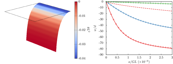
Figure 1: Bending of a square polymer gel plate induced by a vertical edge load with magnitude $a$ applied far from the clamp: comparison between the plate model and the 3D model, for $G\Omega/\mathcal{R}T=0.001$, $\lambda_{\star}=1.5$, $\chi=0.2$. (Left) Deformed equilibrium shape obtained with the plate model for $h/L=0.01$ and $a/GL=3\times 10^{-6}$. The color code represents the dimensionless curvature $\theta L^{2}$ of the midplane, while the black line represents the undeformed configuration of the midplane. (Right) Dimensionless vertical displacement $w/d$ at the tip of the plate as a function of the magnitude of the edge load, for different values of the thickness-to-edge ratio $h/L$: 0.01 (red), 0.014 (blue), 0.03 (green). Solid lines are the results obtained with the 3D model, while circles are the results obtained with the plate model. The dashed line corresponds to the 6-parameter model.

6.2 Swelling–induced wrinkling

The second problem regards the swelling-induced wrinkling of a square polymer gel plate pre-stretched between clamps. A similar problem has been studied in (Lucantonio et al., 2014). First, the clamp-to-clamp distance is increased to fix the nominal strain $\varepsilon=(L^{\prime}-L)/L$, where $L^{\prime}$ is the deformed distance, while keeping the chemical potential of the solvent surrounding the plate unchanged, as in the previous example. We consider nominal strains up to $100\%$, where the large-strain constitutive equations for the plate are crucial to accurately evaluate the initial membranal stress field. At the end of the pre-stretch phase, the plate contracts laterally without developing wrinkles. Then, the chemical potential of the external solvent is increased up to $\mu_{e}=0$, which is higher than the initial chemical potential; as result, the plate absorbs solvent and swells. The constraint imposed by the clamps hampers lateral swelling and thus induces transverse compressive stresses, which trigger the wrinkling instability, as shown in the equilibrium shape of the wrinkled plate depicted in Fig. 2. Compared to the three-dimensional model, the plate model accurately captures amplitude and wavelength of the equilibrium wrinkling pattern, both decreasing with the nominal strain, in agreement with experimental observations.

6.3 Polymer gel composite plates

Inspired by the natural world, where plants adjust their shape by exploiting local changes in swelling, several approaches to shape morphing of polymer gel plates have been proposed. These approaches typically involve the fabrication of polymer gel composite plates (Dickey, 2016), either through the embedding of appropriately oriented reinforcing fibers (Erb et al., 2013; Sydney Gladman et al., 2016), or by introducing a spatial modulation of the cross-linking density of the polymer matrix (Klein et al., 2007; Kim et al., 2012; Wu et al., 2013). In-plane stresses arising from non-homogeneous swelling drive the transformation of the initial, flat configuration into complex, three-dimensional shapes.

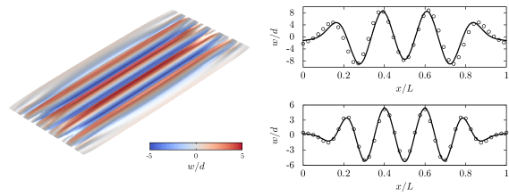
Figure 2: Swelling-induced wrinkling of a square polymer gel plate stretched between clamps: comparison between the plate model and the 3D model, for $G\Omega/\mathcal{R}T=0.001$, $\lambda_{\star}=1.5$, $\chi=0.6$, $h/L=0.001$ and $\mu_{e}=0$. (Left) Deformed equilibrium shape obtained with the plate model for the applied strain $\varepsilon=1.0$. The color code represents the dimensionless vertical displacement of the midplane. (Right) Dimensionless vertical displacement $w/d$ along the line $x/L=1/2$ as a function of the dimensionless transverse coordinate $y/L$, for $\varepsilon=0.5$ (top) and $\varepsilon=1.0$ (bottom). Solid lines and circles are the results obtained with the 3D model and the plate model, respectively.

Here, we study a problem similar to that presented in (Pezzulla et al., 2015). We consider a circular plate consisting of an inner disk with radius $R_{i}$ and a circular annulus with external radius $R_{e}$. The disk and the annulus are made of two polymeric materials with different shear moduli $G_{e}$ and $G_{i}$, respectively, obtained by varying the cross-linking density. We fix the geometrical ratios of the structure as $R_{i}/R_{e}=3/10$, $R_{e}/h=20$, and the solvent-polymer interaction parameter as $\chi=0.2$. The initial swelling of the stiff and soft materials is determined by the swelling ratio $\lambda_{\star}\approx 1.8$. Upon increasing the chemical potential of the external solvent up to $\mu_{e}=0$, incompatible, differential swelling of the disk and the annulus associated with their non-homogeneous stiffness induces compressive stresses that are relieved by out-of-plane buckling.

In the case of stiffer inner disk, the mid-surface of the plate transforms into a saddle-like surface, while in the case of stiffer annulus a dome-like structure is formed, as reported in Fig. 3. As expected, the Gaussian curvature of the deformed mid-surface $K=\det\operatorname{\nabla_{\!s}}\mathbf{n}(s)/\det\widehat{\mathbf{F}}$ is mostly negative (positive) in the saddle-like (dome-like) case.

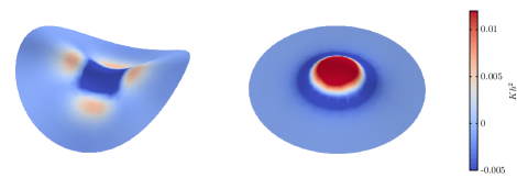
Figure 3: Swelling-induced morphing of saddle-like and dome-like shapes. Deformed equilibrium shapes obtained with the plate model for $G_{e}/G_{i}=3$ (Left) and $G_{e}/G_{i}=1/3$ (Right). The color code represents the dimensionless Gaussian curvature $Kh^{2}$ of the midplane.

7 Conclusions

In conclusion, we have introduced a poroelastic, large-strain plate model that can describe transient, coupled phenomena involving elasticity and solvent migration. The model has been specialized to the case of polymer gels, where the incompressiblity of the polymer matrix and of the solvent induces a kinematic constraint between the volume ratio of the gel and the volume fraction of the solvent. The weak-form plate model has been implemented into a finite element code and its accuracy with respect to the parent three-dimensional model has been demonstrated by several numerical benchmarks. Specifically, we have shown the robustness of the computational model with respect to the analysis of problems involving bifurcations, such as the swelling-induced wrinkling of a pre-stretched membrane and the shape morphing of composite plates.

We consider the present theory to be relevant in computational mechanics of soft, thin structures as a complement to large-strain, elastic plate models. The computational efficiency with respect to three-dimensional models applied to plate-like structures may be exploited in solving optimization problems associated with the design and patterning of gel-based thin structures.

References

- Antman (2005) Antman, S.S., 2005. Nonlinear Problems of Elasticity. Springer.
- Basar and Ding (1996) Basar, Y., Ding, Y., 1996. Finite-element analysis of hyperelastic thin shells with large strains. Computational Mechanics 18, 200–214. URL: http://link.springer.com/article/10.1007/BF00369938, doi:10.1007/BF00369938.
- Basar and Ding (1997) Basar, Y., Ding, Y., 1997. Shear deformation models for large-strain shell analysis. International Journal of Solids and Structures 34, 1687 – 1708. URL: http://www.sciencedirect.com/science/article/pii/S0020768396001217, doi:http://dx.doi.org/10.1016/S0020-7683(96)00121-7.
- Bouklas et al. (2015) Bouklas, N., Landis, C.M., Huang, R., 2015. A nonlinear, transient finite element method for coupled solvent diffusion and large deformation of hydrogels. Journal of the Mechanics and Physics of Solids 79, 21 – 43. URL: http://www.sciencedirect.com/science/article/pii/S0022509615000605, doi:http://dx.doi.org/10.1016/j.jmps.2015.03.004.
- Braun et al. (1994) Braun, M., Bischoff, M., Ramm, E., 1994. Nonlinear shell formulations for complete three-dimensional constitutive laws including composites and laminates. Computational Mechanics 15, 1–18. URL: http://link.springer.com/article/10.1007/BF00350285, doi:10.1007/BF00350285.
- Chester et al. (2015) Chester, S.A., Leo, C.V.D., Anand, L., 2015. A finite element implementation of a coupled diffusion-deformation theory for elastomeric gels. International Journal of Solids and Structures 52, 1 – 18. URL: http://www.sciencedirect.com/science/article/pii/S0020768314003278, doi:http://dx.doi.org/10.1016/j.ijsolstr.2014.08.015.
- Dervaux et al. (2009) Dervaux, J., Ciarletta, P., Ben Amar, M., 2009. Morphogenesis of thin hyperelastic plates: A constitutive theory of biological growth in the föppl–von kármán limit. Journal of the Mechanics and Physics of Solids 57, 458–471. URL: http://linkinghub.elsevier.com/retrieve/pii/S0022509608002093, doi:10.1016/j.jmps.2008.11.011.
- Dias et al. (2011) Dias, M.A., Hanna, J.A., Santangelo, C.D., 2011. Programmed buckling by controlled lateral swelling in a thin elastic sheet. Physical Review E 84, 036603. URL: http://link.aps.org/doi/10.1103/PhysRevE.84.036603, doi:10.1103/PhysRevE.84.036603.
- DiCarlo et al. (2001) DiCarlo, A., Podio-Guidugli, P., Williams, W., 2001. Shells with thickness distension. International Journal of Solids and Structures 38, 1201–1225. URL: http://www.sciencedirect.com/science/article/pii/S0020768300000822, doi:http://dx.doi.org/10.1016/S0020-7683(00)00082-2.
- Dickey (2016) Dickey, M.D., 2016. Hydrogel composites: Shaped after print. Nat Mater 15, 379–380. URL: http://dx.doi.org/10.1038/nmat4608.
- Doi (2009) Doi, M., 2009. Gel dynamics. Journal of the Physical Society of Japan 78, 052001.
- Duda et al. (2010) Duda, F.P., Souza, A.C., Fried, E., 2010. A theory for species migration in a finitely strained solid with application to polymer network swelling. Journal of the Mechanics and Physics of Solids 58, 515 – 529. URL: http://www.sciencedirect.com/science/article/pii/S0022509610000189, doi:http://dx.doi.org/10.1016/j.jmps.2010.01.009.
- Efrati et al. (2009) Efrati, E., Sharon, E., Kupferman, R., 2009. Elastic theory of unconstrained non-Euclidean plates. Journal of the Mechanics and Physics of Solids 57, 762–775. URL: http://linkinghub.elsevier.com/retrieve/pii/S0022509608002160, doi:10.1016/j.jmps.2008.12.004.
- Erb et al. (2013) Erb, R.M., Sander, J.S., Grisch, R., Studart, A.R., 2013. Self-shaping composites with programmable bioinspired microstructures 4, 1712–. URL: http://www.nature.com/doifinder/10.1038/ncomms2666.
- Gemmer and Venkataramani (2013) Gemmer, J., Venkataramani, S.C., 2013. Shape transitions in hyperbolic non-euclidean plates 9, 8151–. URL: http://xlink.rsc.org/?DOI=c3sm50479d.
- Goriely and Ben Amar (2005) Goriely, A., Ben Amar, M., 2005. Differential growth and instability in elastic shells. Phys. Rev. Lett. 94, 198103. URL: http://link.aps.org/doi/10.1103/PhysRevLett.94.198103, doi:10.1103/PhysRevLett.94.198103.
- Hong et al. (2008) Hong, W., Zhao, X., Zhou, J., Suo, Z., 2008. A theory of coupled diffusion and large deformation in polymeric gels. Journal of the Mechanics and Physics of Solids 56, 1779–1793. URL: http://linkinghub.elsevier.com/retrieve/pii/S0022509607002244, doi:10.1016/j.jmps.2007.11.010.
- Kim et al. (2012) Kim, J., Hanna, J.a., Byun, M., Santangelo, C.D., Hayward, R.C., 2012. Designing responsive buckled surfaces by halftone gel lithography. Science 335, 1201–1205. URL: http://www.ncbi.nlm.nih.gov/pubmed/22403385, doi:10.1126/science.1215309.
- Klein et al. (2007) Klein, Y., Efrati, E., Sharon, E., 2007. Shaping of elastic sheets by prescription of non-euclidean metrics. Science 315, 1116–1120. URL: http://www.sciencemag.org/cgi/doi/10.1126/science.1135994, doi:10.1126/science.1135994.
- Lewicka et al. (2010) Lewicka, M., Mahadevan, L., Pakzad, M.R., 2010. The föppl-von kármán equations for plates with incompatible strains. Proceedings of the Royal Society of London A: Mathematical, Physical and Engineering Sciences 467, 402–426. doi:10.1098/rspa.2010.0138.
- Lucantonio et al. (2013) Lucantonio, A., Nardinocchi, P., Teresi, L., 2013. Transient analysis of swelling-induced large deformations in polymer gels. Journal of the Mechanics and Physics of Solids 61, 205–218. doi:10.1016/j.jmps.2012.07.010.
- Lucantonio and Noselli (2016) Lucantonio, A., Noselli, G., 2016. Concurrent factors determine toughening in the hydraulic fracture of poroelastic composites. Meccanica , submitted.
- Lucantonio et al. (2015a) Lucantonio, A., Noselli, G., Trepat, X., DeSimone, A., Arroyo, M., 2015a. Hydraulic fracture and toughening of a brittle layer bonded to a hydrogel. Phys. Rev. Lett. 115, 188105. URL: http://link.aps.org/doi/10.1103/PhysRevLett.115.188105, doi:10.1103/PhysRevLett.115.188105.
- Lucantonio et al. (2014) Lucantonio, A., Roché, M., Nardinocchi, P., Stone, H.A., 2014. Buckling dynamics of a solvent-stimulated stretched elastomeric sheet. Soft Matter 10, 2800. URL: http://xlink.rsc.org/?DOI=c3sm52941j, doi:10.1039/c3sm52941j.
- Lucantonio et al. (2015b) Lucantonio, A., Teresi, L., DeSimone, A., 2015b. Continuum theory of swelling material surfaces with applications to thermo-responsive gels and surface mass transport. Journal of the Mechanics and Physics of Solids doi:10.1016/j.jmps.2016.02.001.
- Noselli et al. (2016) Noselli, G., Lucantonio, A., McMeeking, R.M., DeSimone, A., 2016. Poroelastic toughening in polymer gels: A theoretical and numerical study. Journal of the Mechanics and Physics of Solids 94, 33–46. URL: http://www.sciencedirect.com/science/article/pii/S0022509616301818.
- Pezzulla et al. (2015) Pezzulla, M., Shillig, S.A., Nardinocchi, P., Holmes, D.P., 2015. Morphing of geometric composites via residual swelling. Soft Matter 11, 5812–5820. URL: http://dx.doi.org/10.1039/C5SM00863H.
- Sansour (1995) Sansour, D.I.C., 1995. A theory and finite element formulation of shells at finite deformations involving thickness change: Circumventing the use of a rotation tensor. Archive of Applied Mechanics 65, 194–216. URL: http://link.springer.com/article/10.1007/BF00799298, doi:10.1007/BF00799298.
- Sharon and Efrati (2010) Sharon, E., Efrati, E., 2010. The mechanics of non-euclidean plates. Soft Matter 6, 5693. URL: http://xlink.rsc.org/?DOI=c0sm00479k, doi:10.1039/c0sm00479k.
- Sussman and Bathe (2013) Sussman, T., Bathe, K.J., 2013. 3d-shell elements for structures in large strains. Computers & Structures 122, 2–12. URL: http://www.sciencedirect.com/science/article/pii/S004579491200332X, doi:10.1016/j.compstruc.2012.12.018.
- Sydney Gladman et al. (2016) Sydney Gladman, A., Matsumoto, E.A., Nuzzo, R.G., Mahadevan, L., Lewis, J.A., 2016. Biomimetic 4d printing advance online publication, –. URL: http://www.nature.com/nmat/journal/vaop/ncurrent/full/nmat4544.html.
- Wang and Hong (2012) Wang, X., Hong, W., 2012. A visco-poroelastic theory for polymeric gels. Proceedings of the Royal Society A: Mathematical, Physical and Engineering Sciences 468, 3824–3841. URL: http://rspa.royalsocietypublishing.org/cgi/doi/10.1098/rspa.2012.0385, doi:10.1098/rspa.2012.0385.
- Wu et al. (2013) Wu, Z.L., Moshe, M., Greener, J., Therien-Aubin, H., Nie, Z., Sharon, E., Kumacheva, E., 2013. Three-dimensional shape transformations of hydrogel sheets induced by small-scale modulation of internal stresses. Nature Communications 4, 1586. URL: http://www.nature.com/doifinder/10.1038/ncomms2549, doi:10.1038/ncomms2549.
- Zhang et al. (2009) Zhang, J., Zhao, X., Suo, Z., Jiang, H., 2009. A finite element method for transient analysis of concurrent large deformation and mass transport in gels. Journal of Applied Physics 105, –. URL: http://scitation.aip.org/content/aip/journal/jap/105/9/10.1063/1.3106628, doi:http://dx.doi.org/10.1063/1.3106628.