Log-Concave Duality in Estimation and Control

Abstract

In this paper we generalize the estimation-control duality that exists in the linear-quadratic-Gaussian setting. We extend this duality to maximum a posteriori estimation of the system’s state, where the measurement and dynamical system noise are independent log-concave random variables. More generally, we show that a problem which induces a convex penalty on noise terms will have a dual control problem. We provide conditions for strong duality to hold, and then prove relaxed conditions for the piecewise linear-quadratic case. The results have applications in estimation problems with nonsmooth densities, such as log-concave maximum likelihood densities. We conclude with an example reconstructing optimal estimates from solutions to the dual control problem, which has implications for sharing solution methods between the two types of problems.

1 Introduction

We consider the problem of estimating the state of a noisy dynamical system based only on noisy measurements of the system. In this paper, we assume linear dynamics, so that the progression of state variables is

$$\mathbf{X}_{t+1}= F_{t}(\mathbf{X}_{t})+\mathbf{W}_{t+1},\;\;\;t=0,...,T-1$$ (1)

$$\mathbf{X}_{0}= \mathbf{W}_{0}$$ (2)

$\mathbf{X}_{t}$ is the state variable–a random vector indexed by a discrete time-step $t$ which ranges from $0$ to some final time $T$. All of the results in this paper still hold in the case that the dimension of $\mathbf{X}_{t}$ is time-dependent, but for notational convenience we will assume that $\mathbf{X}_{t}\in\mathbb{R}^{n_{x}}$ for $t=0,...,T$. $F_{t}$ is then a $n_{x}\times n_{x}$ real-valued matrix that, though it may vary with time, is known a priori. The $\mathbf{W}_{t}$ term is a random vector in $\mathbb{R}^{n_{x}}$ that represents noise in the system dynamics. Note that, in this formulation, the random vectors $\mathbf{W}_{t}$ are primitive, in the sense that they generate all of the randomness associated with the problem. The state variables $\mathbf{X}_{t}$ are secondary, being derived from applying dynamic equations to $\mathbf{W}_{t}$ terms.

In addition to the dynamics that govern the state progression, we also have a measurement process which dictates the observable information at time $t$. We assume that the measurement process is linear.

$$\mathbf{Z}_{t}=H_{t}(\mathbf{X}_{t})+\mathbf{V}_{t}$$ (3)

The vector $\mathbf{Z}_{t}$ is a (secondary) random vector of dimension $n_{z}$. Again, we can consider the case that the dimension of $\mathbf{Z}_{t}$ changes with time, but for notational convenience we will assume that the measurements have a fixed dimension. $H_{t}$ is than an $n_{z}\times n_{x}$ matrix, which similar to $F_{t}$ may vary with time but is known in advance. $\mathbf{V}_{t}$ is a primitive random vector of dimension $\mathbb{R}^{n_{z}}$ that represents measurement noise.

Different information structures in this setup correspond to different types of estimation problem. In this paper we consider the smoothing problem, which consists of estimating of $\mathbf{X_{0}},...,\mathbf{X}_{T}$ after all measurement variables $\mathbf{Z}_{0},...\mathbf{Z}_{T}$ have been observed. In this sense, the information associated with the problem is constant–the set of measurements which we use to estimate $\mathbf{X}_{0}$ is the same as the measurements with which we estimate $\mathbf{X}_{T}$ This differs from the filtering problem, which is one of sequential state estimation. In the filtering problem, the set of available measurements depends on the time of the state being estimated. Of course, the difference between these problems can be formulated in terms of measurability with respect to certain filtrations, but we avoid this language because our main problem of interest will end be deterministic.

Kalman, in his seminal paper [9], assumed that there was no measurement noise associated with system, so that $\mathbf{V}_{t}\equiv 0$. Motivated by minimizing mean-squared error, he sought to find the conditional expectation of the states given the measurement. Under the assumption that the dynamic and measurement noise are Gaussian, conditional expectation reduces to a deterministic maximum a posteriori (MAP) problem, in which the optimal estimate is the mode of the conditional density

$$f_{X}(\mathbf{X}_{0},...,\mathbf{X}_{T}|(\mathbf{Z}_{0},...,\mathbf{Z}_{T})=(z_{0},...,z_{T}))$$

Assuming that $\mathbf{W}_{t}\sim\mathcal{N}(0,Q_{t})$ and $\mathbf{V}_{t}\equiv 0$, the problem can be derived explicitly, as in [4]. We are left with the following optimization problem:

$$\min_{x_{0},...,x_{T}} \sum_{t=0}^{T}\frac{1}{2}w_{t}^{\prime}Q_{t}^{-1}w_{t} \mathcal{P}_{Kal}$$ ()

subject to $$x_{t+1}=F_{t}x_{t}+w_{t+1},\;\;t=0,...,T-1$$

$$x_{0}=w_{0}$$

$$z_{t}=H_{t}x_{t},\;\;t=0,...,T$$

In this formulation, the variables $x_{t}$ and $w_{t}$ are estimates of the random variables $\mathbf{X}_{t}$ and $\mathbf{W}_{t}$, respectively. In this sense, $w_{t}$ is also a decision variable, but we prefer to write the problem in this reduced formulation where a decision $x_{0},...,x_{T}$ generates the variables $w_{0},...,w_{T}$.

Kalman observed that the Linear Quadratic Regulator problem

$$\min_{u_{0},...,u_{T}} \sum_{t=0}^{T}\frac{1}{2}y_{t}^{\prime}Q_{t}y_{t} D_{Kal}$$ ()

subject to $$y_{t+1}=F_{t}^{\prime}y_{t}+H_{t}^{\prime}u_{t+1}$$

$$y_{0}=H_{0}^{\prime}u_{0}$$

over controls $\{u_{t}\}_{t=0}^{T}$ and states $\{y_{t}\}_{t=0}^{T}$, is dual to the estimation problem above. Kalman defined this duality in terms of the equations that characterize their solutions: the algebraic Riccati equation which characterizes the value function of ($D_{Kal}$) is the same equation that governs the propagation of the variance of the estimate in ($\mathcal{P}_{Kal}$), with a time reversal. Since the Linear Quadratic Regulator problem is one of optimal control, the relationship between the problems is described as duality between estimation and control, in the Linear-Quadratic Gaussian setting.

Compared to the equation-correspondence duality which is typical in the engineering literature [16], [5] , we take a different approach by using the duality theory of convex programming. The allows us to extend the duality of estimation and control to the more general setting where noise and measurement noise have log-concave densities. This includes the Linear-Quadratic Gaussian framework, but by viewing the duality in a convex-analytic framework we gain more insight into the relationship between estimation and control. Previous literature has focused almost exclusively on either equation-correspondence duality or convex analytic duality between estimation and control problems. We will investigate the relationship between these two notions of duality in a future paper, but for now consider the convex-analytic case.

The rest of this paper is organized as follows. In section 2 we state and prove the main result of the paper: a duality result between estimation and optimal control when the noise terms in (3), (1) are log-concave. Section 3 applies this result to the case where the noise terms have densities which are exponentiated monitoring functions, so that no constraint qualification is required for strong duality. Section 4 contains a practical example, where the solution to the optimal control problem is used to generate an optimal state estimate.

We conclude this section by establishing some definitions and notations that we will use throughout the rest of the paper. Recall that a function is called lower semi-continuous (lsc) if for every $x$ in its domain,

$$\liminf_{x^{\nu}\to x}f(x^{\nu})\geq f(x)$$

for every sequence $x^{\nu}\to x$. In addition, recall that a convex function which takes extended real-values is called proper if it is not identically $\infty$ and never takes the value $-\infty$ [12]. In keeping with convex-analytic literature, we refer to the domain of an extended-valued convex function as the set where it assumes a finite value.

Lastly, given a convex function $f:{\mathbb{R}}^{n}\to(-\infty,\infty]$, we denote by $f^{*}$ the convex conjugate of $f$, which is defined as

$$f^{*}(y)=\sup_{x\in{\mathbb{R}}^{n}}\left\{\langle x,y\rangle-f(x)\right\}.$$

Conjugation is ubiquitous in convex-analytic duality theory, and this paper is no exception. For more details and background on conjugation and its relation to duality, the reader should consult any of [11] [13] [12].

2 Estimation with Convex Penalties

In this section we consider the case where the the random vectors $\mathbf{W}_{t}$ and $\mathbf{V}_{t}$ in (1) and (3) have log-concave density functions. Recall that a function $\phi:{\mathbb{R}}^{d}\to{\mathbb{R}}$ is log-concave if

$$\phi(x)=\exp-f(x)$$

where $f:{\mathbb{R}}^{d}\to(-\infty,\infty]$ is a convex function. By convention, we adopt that $e^{-\infty}=0$.

The collection of random vectors with log-concave densities is broad enough to include many commonly used distributions, such as the normal, Laplace, and exponential [2]. Moreover, it is closed with respect to taking marginals, convolutions, and forming product measures [6]. These characteristics make MAP estimation in the presence of log-concave noise much more amenable to computation than the more general unimodal class, because they guarantee that conditional expectations, sums of random variables, and joint densities formed by independent log-concave random variables remain log-concave. These are exactly the operations performed when considering MAP estimation in the presence of linear dynamics and measurements. The broader class of unimodal distributions, on the other hand, does not enjoy these properties, making them much more difficult to work with in the context of discrete-time state estimation.

Nonparametric density estimation within the class of log-concave random vectors also has attractive theoretical and computational properties. We will not review those results here (see, for example, [7, 10, 15]), but we do comment that the results in the later sections find rich applications in nonparametric log-concave density estimation, particularly because of their non-smooth nature.

The maximum a posteriori estimation of the states, given measurements $z_{0},...,z_{T}$ can be derived similarly to the Gaussian case.

Proposition 2.1.

Assume that $\mathbf{W}_{t}$ and $\mathbf{V}_{t}$ are independent and have log-concave densities $e^{-f_{t}}$ and $e^{-g_{t}}$, respectively, for $t=0,...,T$. Then the maximum a posterior estimate of the states $\mathbf{X}_{0},...,\mathbf{X}_{T}$ given $(\mathbf{Z}_{0},...,\mathbf{Z}_{T})=(z_{0},...,z_{T})$ is given by the solution to the problem

$$\min_{x_{0},...,x_{T}} \sum_{t=0}^{T}f_{t}(w_{t})+\sum_{t=0}^{T}g_{t}(z_{t}-H_{t}x_{t}) \mathcal{P}$$ ()

subject to $$x_{t+1}=F_{t}x_{t}+w_{t+1},\;\;t=0,...,T-1$$

$$x_{0}=w_{0}$$

Equivalently, one can use an extended formulation, minimizing over $w_{t}$ and $x_{t}$, or simply minimizing in $w_{t}$.

Proof.

In maximum a posteriori estimation, we seek to maximize the density

$$p_{\mathbf{X}}(\mathbf{X}_{0},...,\mathbf{X}_{T}|(\mathbf{Z}_{0},...,\mathbf{Z}_{T})=(z_{0},...,z_{n})).$$

By Bayes’ Theorem

$$p_{\mathbf{X}}((\mathbf{X}_{0},...,\mathbf{X}_{T})=(x_{0},...,x_{T})|(\mathbf{Z}_{0},...,\mathbf{Z}_{T})=(z_{0},...,z_{T}))$$

$$=\frac{p_{\mathbf{Z}}((\mathbf{Z}_{0},...,\mathbf{Z}_{T})=(z_{0},...,z_{T})|(\mathbf{X}_{0},...,\mathbf{X}_{T})=(x_{0},...,x_{T}))p_{\mathbf{X}}(\mathbf{X}_{0},...,\mathbf{X}_{T})=(x_{0},...,x_{T}))}{p_{\mathbf{Z}}((\mathbf{Z}_{0},...,\mathbf{Z}_{T})=(z_{0},...,z_{T}))}.$$

By the independence of measurement noise,

$$p_{\mathbf{Z}}((\mathbf{Z}_{0},...,\mathbf{Z}_{T})=(z_{0},...,z_{T})|(\mathbf{X}_{0},...,\mathbf{X}_{T})=(x_{0},...,x_{T}))=\prod_{t=0}^{T}p_{\mathbf{V}_{t}}(z_{t}-H_{t}x_{t}).$$

Furthermore, since the process is Markov (by independence of dynamic noise)

$$p_{\mathbf{X}}((\mathbf{X}_{0},...,\mathbf{X}_{T})=(x_{0},...,x_{T}))=p_{\mathbf{X}_{0}}(x_{0})\cdot p_{\mathbf{X}_{1}}(x_{1}|x_{0})\cdot...\cdot p_{\mathbf{X}_{T}}(x_{T}|x_{T-1}).$$

Our posterior becomes

$$\frac{\prod_{t=0}^{T}p_{\mathbf{V}_{t}}(z_{t}-H_{t}x_{t})\cdot p_{\mathbf{X}_{0}}(x_{0})\cdot\prod_{t=1}^{T}p_{\mathbf{X}_{t}}(x_{t}|x_{t-1})}{p_{\mathbf{Z}}((\mathbf{Z}_{0},...,\mathbf{Z}_{T})=(z_{0},...,z_{T}))}.$$

By the assumptions on the distributions of $\mathbf{V}_{t}$ and $\mathbf{W}_{t}$, this is

$$C(z_{0},...,z_{T})\cdot\exp\left\{-f_{0}(x_{0})-\sum_{t=0}^{T-1}f_{t+1}(x_{t+1}-F_{t}(x_{t}))-\sum_{t=0}^{T}g_{t}(z_{t}-H_{t}x_{t})\right\}$$

where $C(z_{0},...,z_{n})$ is some term not depending on $(x_{0},...,x_{T})$. Maximizing this expression in $(x_{0},...,x_{T})$ is then equivalent to minimizing

$$f_{0}(x_{0})+\sum_{t=0}^{t-1}f_{t+1}(x_{t+1}-F_{t}(x_{t}))+\sum_{t=0}^{T}g_{t}(z_{t}-H_{t}(x_{t})).$$

This gives us the problem in the statement of the proposition. The different formulations follow because each choice of $(x_{0},,,x_{T})$ generates a unique $(w_{0},...,w_{T})$, according to the dynamics, and vice versa. ∎

The extension from the Gaussian noise to log-concave random vectors is signficant. The fact that the functions $f_{t}$ and $g_{t}$ in $\mathcal{P}$ can take the value $\infty$ permits a choice of densities which do not have full support. Correspondingly, the MAP problem then becomes one of traditional convex optimization [13], [12], where constraints are built in to the objective function by allowing that function to take infinite values.

The next lemma provides information about the function $f$ used to define a log-concave density.

Lemma 2.2.

Assume that $f:\mathbb{R}^{n}\to\overline{\mathbb{R}}$ is a convex function which defines the density of a random variable $\mathbf{X}\sim e^{-f(x)}$. Then

1. If ${\mathrm{cl}\,}(f)$ is the lower-semicontinuous hull of $f$, then $e^{{\mathrm{cl}\,}(f)}$ is also a density function for $\mathbf{X}$.

2. $f$ is proper

3. $dom(f)$ is full-dimensional

4. $f$ is level-bounded, so that the minimum of $f$ over $\mathbb{R}^{n}$ is attained.

Proof.

First we prove (a). Since a convex function is continuous on the interior of its domain [13][10.1], the only points where $f$ may fail to be lower semicontinuous is on the boundary of its domain. The domain of a convex function is obviously convex, and since the boundary of a convex set has Lebesgue measure zero [8][Lemma 1.8.1], ${\mathrm{cl}\,}(f)$ and $f$ are equal almost everywhere. Hence $e^{{\mathrm{cl}\,}(f)}$ is also a density function for $X$, since it differs from the given density on a set of measure zero. This results allows us to refer to pointwise values of $f$, by which we mean the values of the unique lower-semicontinuous extension ${\mathrm{cl}\,}(f)$.

(b) follows from (a) and the fact that $\int e^{-f(x)}dx=1$. Because an improper lower-semicontinuous convex function can have no finite values [13][Cor 7.2.1], $f$ must be proper in order for $e^{-f(x)}$ to integrate to one.

For (c), if $dom(f)$ were not full dimensional then it is a subset of a proper affine subspace of $\mathbb{R}^{n}$. This set has measure zero, which violates the condition that $e^{-f(x)}$ integrates to one.

Lastly, we prove (d). In order that $\int e^{-f(x)}dx=1$, we must have $f(x)\to\infty$ as $\left|x\right|\to\infty$. This means that $f$ is level bounded, which combined with the fact that we can without loss of generality take $f$ to be lower-semicontinuous, gives that $f$ attains its minimum [12][Thm 1.9] ∎

To simplify calculations in the results that follow, we will rewrite the problem $\mathcal{P}$ in a more compact form. We borrow from Rockafellar [14] the notion of a supervector, which is simply a concatenated vector consisting of a variable at all time steps. Let $w=(w_{0},...,w_{T})^{\prime}$, $z=(z_{0},...,z_{T})^{\prime}$, $x=(x_{0},...,x_{T})^{\prime}$ be the supervectors corresponding MAP estimates of the dynamical noise, measurements, and states, respectively. Define

$$f(w)=\sum_{t=0}^{T}f_{t}(w_{t}),$$

$$g(z)=\sum_{t=0}^{T}g_{t}(z_{t}).$$

Note that each of these functions is separable with respect to the components of their respective supervectors. Hence infimums and supremums can be performed with respect to each component.

Define

$$A=\left(\begin{array}[]{cccc}1&0&\cdots&0\\ -F_{0}&1&\cdots&0\\ 0&\ddots&\ddots&0\\ 0&\cdots&-F_{T-1}&1\end{array}\right)$$

so that the dynamical system constraint in $\mathcal{P}$ can be represented as

$$Ax-w=0.$$ (4)

Similarly, let

$$H=\left(\begin{array}[]{cccc}H_{0}&0&\cdots&0\\ 0&H_{1}&\cdots&\\ \vdots&\vdots&\ddots&\vdots\\ 0&0&\cdots&H_{T}\end{array}\right).$$

Then the measurement constraint can be rewritten in supervector notation as well, allowing us to rewrite problem $\mathcal{P}$

$$\min_{x,w} \quad f(w)+g(z-Hx)$$ (5)

s.t. $$Ax-w=0.$$

We now turn our attention to convex-analytic duality. For concreteness, we assume that $C\subseteq\mathbb{R}^{n}$ and $D\subseteq\mathbb{R}^{m}$. Recall that a convex problem $\min_{x\in C}h(x)$ is dual to a concave problem $\max_{y\in D}k(y)$ if there is a convex-concave function $L:\mathbb{R}^{n}\times\mathbb{R}^{m}\to\overline{\mathbb{R}}$ such that

$$h(x)=\sup_{y\in D}L(x;y)\;\;\;\text{ and }\;\;\;k(y)=\inf_{x\in C}L(x;y).$$

This definition, from [11], is equivalent to the notion of duality in which one perturbs constraints in order to generate a saddle function $L$. Indeed, a perturbation function $F$ can be generated from the equation

$$F(x,u)=\sup_{y\in D}\left\{K(x,y)-u^{\prime}y\right\}.$$

Of course, this duality framework subsumes the familar Lagrangian duality, Fenchel duality, and various other duality schemes. We refer the reader to [11] for details and examples, and focus on applying this theory to the problem at hand.

Theorem 2.3.

When $f$ and $g$ are convex, problem ($\mathcal{P}$) is the primal problem associated with the saddle function

$$L(w,x;u,y)=f(w)+z^{\prime}u-g^{*}(u)-u^{\prime}Hx+y^{\prime}(Ax-w)$$

on $C:={\mathbb{R}}^{(T+1)\times n_{x}}\times{\mathbb{R}}^{(T+1)\times n_{x}}$, $D:={\mathbb{R}}^{(T+1)\times n_{z}}\times{\mathbb{R}}^{(T+1)\times n_{x}}$

Proof.

To prove that ($\mathcal{P}$) is the primal problem for the saddle-function $L$, we will show that

$$\eqref{prob:EstConv}=\min_{(w,x)\in C}\sup_{(u,y)\in D}L(w,x;u,y)$$

which satisfies the definition in [11]. For ease of notation, in what follows we omit the sets over which we take the infimums and supremums. By the separability of $L$,

$$\sup_{u,y}L(w,x;u,y)=f(w)+\sup_{u}\left\{u^{\prime}(z-Hx)-g^{*}(u)\right\}+\sup_{y}\left\{y^{\prime}(Ax-w)\right\}$$

Obviously the right-most supremum is $0$ when $Ax-w=0$ and $\infty$ otherwise. Furthermore, Lemma 2.2 gives that without loss of generality $g$ is proper and lsc. Therefore the Fenchel-Moreau Theorem [12, Th 11.1] gives that

$$\sup_{u}\left\{u^{\prime}(z-Hx)-g^{*}(u)\right\}=g^{**}(z-Hx)=g(z-Hx).$$

Thus

$$\min_{w,x}\sup_{u,y}L(w,x;u,y)$$

$$=\min_{w,x} f(w)+g(z-Hx)$$

s.t. $$Ax-w=0$$

∎

Theorem 2.4.

The dual problem associated with $L$ on ${\mathbb{R}}^{(T+1)\times n_{x}}\times{\mathbb{R}}^{(T+1)\times n_{x}}$, ${\mathbb{R}}^{(T+1)\times n_{z}}\times{\mathbb{R}}^{(T+1)\times n_{x}}$ is

$$\sup_{y,u}\; z^{\prime}u-f^{*}(y)-g^{*}(u)$$ (6)

s.t. $$A^{\prime}y-H^{\prime}u=0$$

Furthermore, this problem has an equivalent reduced formulation where the supremum is taken over $u$.

Proof.

The dual problem associated with the triple $L$, ${\mathbb{R}}^{(T+1)\times n_{x}}\times{\mathbb{R}}^{(T+1)\times n_{x}}$, ${\mathbb{R}}^{(T+1)\times n_{z}}\times{\mathbb{R}}^{(T+1)\times n_{x}}$ is

$$\sup_{u,y}\inf_{w,x}L(w,x;v,y)$$

$$= \sup_{u,y}\inf_{w,x}f(w)+z^{\prime}u-g^{*}(u)-u^{\prime}Hx+y^{\prime}(Ax-w)$$

$$= \sup_{u,y}\inf_{w,x}f(w)-w^{\prime}y+x^{\prime}(A^{\prime}y-H^{\prime}u)+z^{\prime}u-g^{*}(u)$$

$$= \sup_{u,y}z^{\prime}u-g^{*}(u)+\inf_{w}\left\{f(w)-w^{\prime}y\right\}+\inf_{x}\{x^{\prime}(A^{\prime}y-H^{\prime}u)\}$$

$$=\sup_{u,y} z^{\prime}u-g^{*}(u)-f^{*}(y)$$

s.t. $$A^{\prime}y-H^{\prime}u=0$$

Lastly, the equivalent reduced formulation follows because the each $u$ generates a unique $y$ vector according to the constraints. ∎

Appealing to the separability of $f$ and $g$, and expanding the matrices $A^{\prime}$ and $H^{\prime}$, we have established the following main result.

Theorem 2.5.

The dual problem associated with the estimation problem ($\mathcal{P}$) is the optimal control problem

$$\sup_{u_{0},...,u_{T}} \sum_{t=0}^{T}f_{t}^{*}(y_{t})+g_{t}^{*}(u_{t})-z_{t}^{\prime}u_{t} \mathcal{D}$$ ()

s.t. $$y_{t}=F_{t}^{\prime}y_{t+1}+H^{\prime}_{t}u_{t},\;\;t=0,...,T-1$$

$$y_{T}=H^{\prime}u_{T}$$

The next theorem provides a condition, known as a constraint qualification, for strong duality to hold between the estimation problem $\mathcal{P}$ and control 6 problems above.

Theorem 2.6.

[13, Theorem 28.2] Assume that the problem $\mathcal{P}$ is strictly feasible, so that there exists a pair $(x,w)$ satisfying (4), $w\in\text{int}(\text{dom}(f))$, $z-Hx\in\text{int}(\text{dom}(g))$. Then a strong duality relationship exists between the problems $\mathcal{P}$ and $\mathcal{D}$. In other words, the supremum in $\mathcal{D}$ equals the optimal value in $\mathcal{P}$. Furthermore, this supremum is attained.

Proof.

This follows directly from the strong duality theorem in [13, Theorem 28.2]. Note that the typical formulation of this constraint qualification requires only a relative interior point, when the domains are considered as subsets of their affine hulls, instead of an interior point. However, since by Lemma 2.2 the domains of $f$ and $g$ are full-dimensional, the notions are equivalent. ∎

sectionThe Piecewise Linear Quadratic Case

In this section we investigate structural constraints on the functions $f_{t}$ and $g_{t}$ in the densities of $\mathbf{W}_{t}$ and $\mathbf{V}_{t}$ that allow us to remove the constraint qualification condition in 2.6.

Recall that a function is linear-quadratic if it is polynomial of degree at most two, so that constant and linear functions are included in this family.

Theorem 2.7.

Assume that $f_{t}$ and $g_{t}$ are convex and piecewise linear-quadratic. If either $\mathcal{P}$ or $\mathcal{D}$ are feasible, then strong duality holds between these estimation and optimal contorl problems, so that their optimal objective values are equal. Furthermore, both problems attain their optimal objective values.

Proof.

If $f_{t}$ and $g_{t}$ are piecewise linear quadratic, then the reformulated problem 5 is a piecewise linear-quadratic program. Lemma 2.2 gives us that each of $f_{t}$ and $g_{t}$ are proper, and hence each of their conjugates is as well. Combined with the assumption that one of $\mathcal{P}$ and $\mathcal{D}$ is feasible, we know that the optimal objective value of this problem is finite. Strong duality and the attaining of optimal values then follow directly from [12][Thm 11.42] ∎

Theorem 2.7 removes the contraint qualification of Theorem 2.5 by imposing extra structure on the functions $f_{t}$ and $g_{t}$. By assuming that $f_{t}$ and $g_{t}$ are piecewise linear-quadratic, strong duality becomes automatic.

When $f_{t}$ and $g_{t}$ are arbitrary convex functions, computing closed form expressions for the conjugates that occur in the dual problem may be difficult. The conjugate function, Lagrangian, and dual problem $\mathcal{D}$ are especially easy to compute in the special case that $f_{t}$ and $g_{t}$ are monitoring functions, which includes many problems of practical interest.

A monitoring function is a function $\rho_{U,M}:\mathbb{R}^{n}\to\overline{\mathbb{R}}$ defined by

$$\rho_{U,M}(x)=\sup_{u\in U}\{x^{\prime}u-\frac{1}{2}u^{\prime}Mu\}$$

where $U\subseteq\mathbb{R}^{n}$ is a nonempty polyhedral set and $M$ is an $n\times n$ positive semidefinite matrix.

Monitoring functions are flexible tools for modeling penalties. They are proper, convex, and piecewise linear-quadratic [12][Ex 11.18], and can be used to model a variety of linear and quadratic penalties in addition to polyhedral constraints. A probabilistic interpretation of the use of monitoring functions in robust smoothing problems can be found in [1]. The authors detail the construction of many commonly used penalties in robust optimization, and provide remarks for constructing others.

The incentive for considering the case that $f_{t}$ and $g_{t}$ are monitoring functions is two-fold. The first is that, though this is requires a further restriction on the form of $f_{t}$ and $g_{t}$, the MAP problem Gaussian noise is contained in this case. The second is that the framework provides enough structure to make the computation of the conjugates and the dual control problem $\mathcal{D}$ straight-forward.

We’ll be aided in this by the following lemma.

Lemma 2.8.

If $\rho_{U,M}$ is a monitoring function, then the conjugate $\rho^{*}_{U,M}$ is given by

$$\rho^{*}_{U,M}(y)=\left\{\begin{array}[]{cc}\frac{1}{2}y^{\prime}My&\text{ when }y\in U\\ \infty&\text{ otherwise}\end{array}\right.$$

Proof.

$$\rho^{*}_{U,M}(y) =\sup_{x\in\mathbb{R}^{n}}\left\{x^{\prime}y-\rho_{U,M}(x)\right\}$$

$$=\sup_{x\in\mathbb{R}^{n}}\left\{x^{\prime}y-\sup_{u\in U}\left\{x^{\prime}u-\frac{1}{2}u^{\prime}Mu\right\}\right\}$$

$$=\sup_{x\in\mathbb{R}^{n}}\inf_{u\in U}\left\{x^{\prime}(y-u)+\frac{1}{2}u^{\prime}Mu\right\}$$ (7)

This can be interpreted as the dual to the problem

$$\inf_{u\in U} \frac{1}{2}u^{\prime}Mu$$

s.t. $$u=y$$

In the same spirit as 2.7, we apply [12][11.42] to see that, when $U$ is nonempty, 2 equals

$$\inf_{u\in U}\sup_{x\in\mathbb{R}^{n}} \left\{x^{\prime}(y-u)+\frac{1}{2}u^{\prime}Mu\right\}$$

$$=\left\{\begin{array}[]{cc}\frac{1}{2}y^{\prime}My&\text{ when }y\in U\\ \infty&\text{ otherwise}\end{array}\right.$$

∎

We’ve arrived at a precise formulation of the dual control problem $\mathcal{D}$.

Corollary 2.9.

If $\mathbf{W}_{t}$ and $\mathbf{V}_{t}$ have a PLQ density

$$\mathbf{W}_{t}\propto e^{-\rho_{W_{t},M_{t}}}\;\;\;\mathbf{V}_{t}\propto e^{-\rho_{V_{t},N_{t}}}$$

with $M_{t},N_{t}\succeq 0$ and and $W_{t}$, $V_{t}$ nonempty and polyhedral, then the MAP problem $\mathcal{P}$ is dual to the control problem

$$\sup_{u_{0},...,u_{T}} \sum_{t=0}^{T}\frac{1}{2}y_{t}^{\prime}M_{t}y_{t}+\frac{1}{2}u_{t}^{\prime}N_{t}u_{t}-z_{t}^{\prime}u_{t}$$ (8)

s.t. $$y_{t}=F_{t}^{\prime}y_{t+1}+H^{\prime}_{t}u_{t},\;\;t=0,...,T-1$$

$$y_{T}=H^{\prime}u_{T}$$

$$y_{t}\in W_{t},\;\;\;t=0,...,T$$ (9)

$$u_{t}\in V_{t},\;\;\;t=0,...,T$$ (10)

Optimal values are attained and strong duality holds when either problem is feasible.

Proof.

Follows directly from 2.5 and 2.7. ∎

As an application of Theorem 2.9, we verify the strong duality between estimation and control in the linear-quadratic Gaussian setting. By taking $\mathbf{W}_{t}\sim\mathcal{N}(0,Q_{t})$ and $\mathbf{V}_{t}\sim\mathcal{N}(0,R_{t})$, we can represent the density functions as in theorem 2.9 by taking

$$W_{t}=\mathbb{R}^{n_{x}},\;M_{t}=Q_{t},\;\;\;\;V_{t}=\mathbb{R}^{n_{z}},N_{t}=R_{t}$$

Because $\rho_{t,\mathbb{R}^{n_{x}},Q_{t}}$ and $\rho_{t,\mathbb{R}^{n_{z}},R_{t}}$ have domains $\mathbb{R}^{n_{x}}$ and $\mathbb{R}_{n_{z}}$, respectively, the MAP problem is feasible for any measurements $(z_{0},...,z_{T})$. Strong duality then follows directly from Theorem 2.9.

Moreover, by taking $\mathbf{W}_{t}\sim\mathcal{N}(0,Q_{t})$ and $\mathbf{V}_{t}\equiv 0$, we recover the duality of the two problems considered by Kalman from the introduction. The time reversal is in fact an artifact of taking the convex analytic dual, though recovery of the Riccati-covariance propagation equivalence requires considering each problem as sequential, which is not the appoach that we’ve taken here.

3 Applications: Reconstructing an Estimator from Optimal Controls

In this section we apply the results of the previous sections to construct the solution to an optimal estimation problem from the solution to its dual problem of optimal control. We focus on a nonsmooth problem of practical interest. First, we formulate an estimation problem where the density of the measurement noise is generated via log-concave maximum likelihood estimation from a sample of measurement noise. We then use the result 2.5 to construct a corresponding dual control problem. Finally, we use the solution to this control problem to construct an optimal estimator for the original problem.

The set up for this problem motivated by the following scenario. A practioner aims to estimate the current and previous states of a dynamical system from a set of noisy measurements. Through calibration of a sensor or observation, the practioner has the ability to generate sample data for the measurement noise. How can one use this data to formulate an estimation problem which reflects the tendencies of the sensor? We would like to capitalize on the ability to generate measurement noise, instead of defaulting to a Gaussian noise assumption.

The following theorem, due to [15] and [10], as well as the computational results in [7], allow us to form a nonparametric density estimate of a log-concave density based on a set of sample data.

Theorem 3.1.

If $X_{1},...,X_{n}$ are i.i.d. observations from a univariate log-concave density, then the nonparamtric MLE exists, is unique, and is of the form $\hat{\phi}_{n}=\exp\hat{f_{n}}$. The function $\hat{f}_{n}$ is piecewise linear on $[X_{(1)},X_{(n)}]$, with the set of knots contained in $\{X_{1},...,X_{n}\}$. Outside of $[X_{(1)},X_{(n)}]$, $\hat{f}$ takes the value $\infty$.

For the generation of our example problem, we use 10 time steps and a two dimensional state space, motivated by components representing position and velocity. The dynamics matrices $F_{t}$ corresponds to the physical dynamics that would occur in such a situation. We produce a “true” sequence of states to be estimated by generating dynamical system noise according to a $\mathcal{N}(0,I)$ distribution. We take the measurement operators $H_{t}$ be the sum of the components. Lastly, we construct measurements from a sample of Laplace$(0,1)$ measurement noise.

For the formulation of the MAP problem, we assume that the dynamical system noise was generated according to $\mathcal{N}(0,I)$ distribution. For the measurement noise, we construct a log-concave MLE estimator $e^{-\hat{g}}$ of the density from a sample of size 100 generated from a Laplace(0,1) distribution. $\hat{g}$ and its convex conjugate $\hat{g}^{*}$ are illustrated in figure 1.

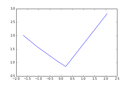
(a) $\hat{g}$

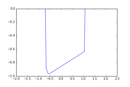
(b) $\hat{g}^{*}$

Figure 1: $\hat{g}$ and $\hat{g}^{*}$, where the MLE density is $e^{-g(x)}$

The MAP problem $\mathcal{P}$ is then

$$\min_{x_{0},...,x_{10}} \sum_{t=0}^{10}\frac{1}{2}\left|\left|w_{t}\right|\right|^{2}+\hat{g}(z_{t}-(\begin{array}[]{cc}1&1\end{array})\cdot x_{t})$$

s.t. $$x_{t+1}=\left(\begin{array}[]{cc}1&1\\ 0&1\end{array}\right)x_{t}+w_{t+1},\;\;\;t=0,...,T-1$$

$$x_{0}=w_{0}$$

According to 2.5 this problem has as its dual the control problem

$$\max_{u_{0},...,u_{10}} \sum_{t=0}^{10}\frac{1}{2}\left|\left|y_{t}\right|\right|^{2}+\hat{g}^{*}(u_{t})-u_{t}^{\prime}z_{t} \mathcal{D}_{ex}$$ ()

s.t. $$y_{t}=\left(\begin{array}[]{cc}1&0\\ 1&1\end{array}\right)y_{t+1}+\left(\begin{array}[]{c}1\\ 1\end{array}\right)u_{t},\;\;\;t=0,...,T-1$$

$$y_{T}=\left(\begin{array}[]{c}1\\ 1\end{array}\right)u_{T}$$

Because our dynamical system noise in 3 has full support, Theorem 2.6 guarantees that strong duality holds between the problems, and that the dual control problem attains its solution. Assume that we have solved this control problem and have a corresponding optimal control $(u^{*},y^{*})$. Since an optimal estimate $(w^{*},x^{*})$ gives a saddle point $(w^{*},x^{*};u^{*},y^{*})$ to the Lagrangian $L$ in Theorem 2.4, it follows from the proof of this theorem that $w^{*}$ minimizes $f(w)-w^{\prime}y^{*}$. In our problem $f$, when $f(w)=\frac{1}{2}\left|\left|w\right|\right|^{2}$, which yields the relationship $w^{*}=y^{*}$. This is similar to the relationship between primal and dual solutions in the Fenchel Duality framework. See [3][Prop. 5.3.8] for further details. Note that this allows us to reconstruct a primal solution from a dual solution and vice versa. In particular, the relationship between $y^{*}$ and $w^{*}$ is linear when the dynamical system noise is assumed to be Gaussian.

Solving $\mathcal{D}_{ex}$ to optimality gives $y^{*}$, from which we generate $w^{*}$ and then an optimal estimate $x^{*}$. Figure 2 contains a plot of the estimated and true state.

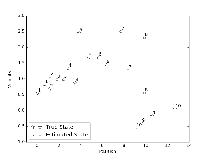
Figure 2: Dual Reconstruction of State Estimate

Though we have demonstrated a convenient technique to generate solutions for an estimation problem from the solution to its dual control problem, in this example we have no reason to believe that solving $\mathcal{D}_{ex}$ is any easier than solving the original problem 3. Nevertheless, the results in this and previous sections provide motivation for further investigation into applying control algorithms to solve estimation problems and vice versa.

References

- [1] Aleksandr Y Aravkin, James V Burke and Gianluigi Pillonetto “Sparse/robust estimation and kalman smoothing with nonsmooth log-concave densities: Modeling, computation, and theory” In The Journal of Machine Learning Research 14.1 JMLR. org, 2013, pp. 2689–2728
- [2] Mark Bagnoli and Ted Bergstrom “Log-concave probability and its applications” In Economic theory 26.2 Springer, 2005, pp. 445–469
- [3] Dimitri P Bertsekas “Convex optimization theory” Athena Scientific Belmont, 2009
- [4] Henry Cox “On the estimation of state variables and parameters for noisy dynamic systems” In Automatic Control, IEEE Transactions on 9.1 IEEE, 1964, pp. 5–12
- [5] M.H.A. Davis “Linear estimation and stochastic control”, Chapman and Hall mathematics series ChapmanHall, 1977 URL: https://books.google.com/books?id=QgIqAQAAMAAJ
- [6] Sudhakar Dharmadhikari and Kumar Joag-Dev “Unimodality, convexity, and applications” Elsevier, 1988
- [7] Lutz Dümbgen and Kaspar Rufibach “logcondens: Computations Related to Univariate Log-Concave Density Estimation”
- [8] Krzysztof Jarosz “Function Spaces in Analysis” American Mathematical Society, 2015
- [9] Rudolph Emil Kalman “A New Approach to Linear Filtering and Prediction Problems” In Transactions of the ASME–Journal of Basic Engineering 82.Series D, 1960, pp. 35–45
- [10] Jayanta Kumar Pal, Michael Woodroofe and Mary Meyer “Estimating a Polya Frequency Function₂” In Lecture Notes-Monograph Series JSTOR, 2007, pp. 239–249
- [11] R Tyrrell Rockafellar “Conjugate duality and optimization” SIAM, 1974
- [12] R Tyrrell Rockafellar and Roger J-B Wets “Variational analysis” Springer Science & Business Media, 2009
- [13] Ralph Tyrell Rockafellar “Convex analysis” Princeton university press, 2015
- [14] RT Rockafellar “Duality and optimality in multistage stochastic programming” In Annals of Operations Research 85 Springer, 1999, pp. 1–19
- [15] Kaspar Rufibach “Log-concave Density Estimation and Bump Hunting for iid Observations”, 2006
- [16] Emanuel Todorov “General duality between optimal control and estimation” In Decision and Control, 2008. CDC 2008. 47th IEEE Conference on, 2008, pp. 4286–4292 IEEE