Real-Time Anomaly Detection for Streaming Analytics
Abstract
Much of the world’s data is streaming, time-series data, where anomalies give significant information in critical situations. Yet detecting anomalies in streaming data is a difficult task, requiring detectors to process data in real-time, and learn while simultaneously making predictions. We present a novel anomaly detection technique based on an on-line sequence memory algorithm called Hierarchical Temporal Memory (HTM). We show results from a live application that detects anomalies in financial metrics in real-time. We also test the algorithm on NAB, a published benchmark for real-time anomaly detection, where our algorithm achieves best-in-class results.
1 Introduction
Across every industry, we are seeing an exponential increase in the availability of streaming, time-series data. Largely driven by the rise of the Internet of Things (IoT) and connected real-time data sources, we now have an enormous number of applications with sensors that produce important, continuously changing data.
The detection of anomalies in real-time streaming data has practical and significant applications across many industries. There are numerous use cases for anomaly detection, including preventative maintenance, fraud prevention, fault detection, and monitoring. The use cases can be found throughout numerous industries such as finance, IT, security, medical, energy, e-commerce, and social media.
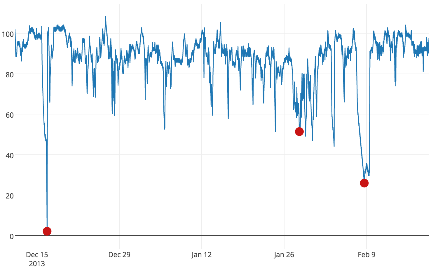
We define an anomaly as a point in time where the behavior of the system is unusual and significantly different from past behavior. Under this definition, an anomaly does not necessarily imply a problem. A change might be for a negative reason like the temperature sensor on an engine going up, indicating a possible imminent failure. Or the change might be for a positive reason like web clicks on a new product page are abnormally high, showing strong demand. Either way, the data is unusual and may require action. Anomalies can be spatial, meaning the value is outside the typical range like the first and third anomalies in Figure 1. They can also be temporal, where the value isn’t outside the typical range but the sequence in which it occurs is unusual. The middle anomaly in Figure 1 is a temporal anomaly.
Real-time applications impose their own unique constraints for machine learning. Anomaly detection in streaming applications is particularly challenging. The detector must process data and output a decision in real-time, rather than making many passes through batches of files. In most scenarios the number of sensor streams is large and there is little opportunity for human, let alone expert, intervention. As such, operating in an unsupervised, automated fashion (e.g. without manual parameter tweaking) is often a necessity. The underlying system is often non-stationary, and detectors must continuously learn and adapt to changing statistics while simultaneously making predictions.
The goal of this paper is to introduce a novel anomaly detection technique designed for such real-time applications. We show how to use Hierarchical Temporal Memory (HTM) networks (Hawkins & Ahmad, 2016; Padilla et al., 2013; Rozado et al., 2012) in a principled way to robustly detect anomalies in a variety of conditions. The resulting system is efficient, extremely tolerant to noisy data, continously adapts to changes in the statistics of the data, and detects very subtle anomalies while minimizing false positives. We show qualitative examples from a real-time financial anomaly detection application. We also report leading results on an open benchmark for real-time anomaly detection. The algorithm has been deployed commercially, and we discuss some of the practical lessons learned from these deployments. We have made the complete source code (including end application code) available in open source repositories 111Please see http://numenta.org.
2 Related Work
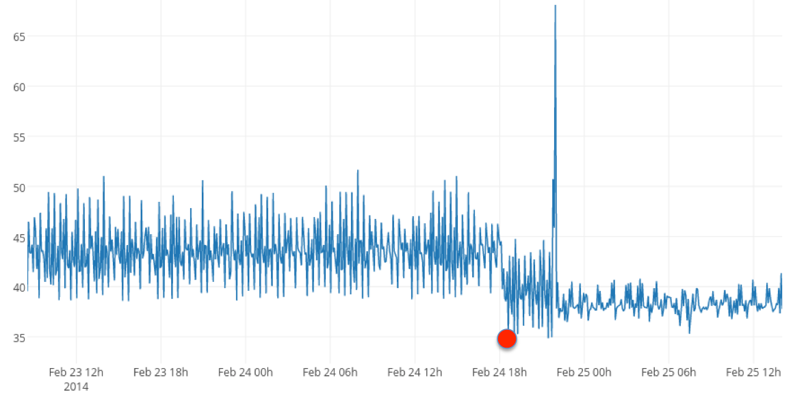
Anomaly detection in time-series is a heavily studied area, dating back to (Fox, 1972). Some techniques, like classification-based methods, are supervised or semi-supervised. While labelled data can be used to improve results, supervised techniques are typically unsuitable for anomaly detection (Görnitz et al., 2013). Figure 2 illustrates the need for continuous learning, which is not typically possible with supervised algorithms.
Other techniques, like simple thresholds, clustering, and exponential smoothing, are only capable of detecting spatial anomalies. Holt-Winters is an example of the latter that is commonly implemented for commercial applications (Szmit & Szmit, 2012). Also commonly used in practice are change point detection methods, which are capable of identifying temporal anomalies. The typical approach is to model the time series in two independent moving windows and detect when there is a significant deviation in the time series metrics (Basseville & Nikiforov, 1993). These methods are often extremely fast to compute and have low memory overhead. The detection performance of these statistical techniques can be sensitive to the size of the windows and thresholds. This sometimes results in many false positives as the data changes, requiring frequent updates to the thresholds in order to detect anomalies while minimizing false positives.
The Skyline project provides an open source implementation of a number of statistical techniques for detecting anomalies in streaming data (Stanway, 2013). The different algorithms can be combined into an ensemble. The Skyline algorithms are included in our results.
There are other algorithms capable of detecting temporal anomalies in complex scenarios. ARIMA is a general purpose technique for modeling temporal data with seasonality (Bianco et al., 2001). It is effective at detecting anomalies in data with regular daily or weekly patterns. It is not capable of dynamically determining the period of seasonality, although extensions have been developed for doing so (Hyndman & Khandakar, 2008). A technique for applying ARIMA to multivariate data has also been studied (Tsay, 2000). Bayesian change point detection methods are a natural approach to segmenting time series and can be used for online anomaly detection (Adams & Mackay, 2007; Tartakovsky et al., 2013). Some additional techniques for general purpose anomaly detection on streaming data include (Keogh et al., 2005; Rebbapragada et al., 2009).
Yahoo released the open source EGADS framework for time series anomaly detection that pairs time series forecasting techniques with common anomaly detection algorithms (Laptev et al., 2015). Twitter released its own open source anomaly detection algorithms for time series data (Kejariwal, 2015). Both are capable of detecting spatial and temporal anomalies. Empirical comparison with Twitter’s detection software are included in our results.
There have been a number of model-based approaches applied to specific domains. These tend to be extremely specific to the domain they are modeling. Examples include anomaly detection in aircraft engine measurements (Simon & Rinehart, 2015), cloud datacenter temperatures (Lee et al., 2013), and ATM fraud detection (Klerx et al., 2014). While these approaches may have success in a specific domain, they are not suitable for general purpose applications.
We have reviewed some of the algorithms most relevant to our work. A comprehensive literature review is outside the scope of this paper but there are several thorough reviews of anomaly detection techniques for further reading (Chandola et al., 2009; Hodge & Austin, 2004; Chandola et al., 2008).
In this paper we focus on using Hierarchical Temporal Memory (HTM) for anomaly detection. HTM is a machine learning algorithm derived from neuroscience that models spatial and temporal patterns in streaming data (Hawkins & Ahmad, 2016; Rozado et al., 2012). HTM compares favorably with some state of the art algorithms in sequence prediction, particularly complex non-Markovian sequences (Cui et al., 2015; Padilla et al., 2013). HTMs are continuously learning systems that automatically adapt to changing statistics, a property particularly relevant to streaming analytics.
3 Anomaly Detection Using HTM
Typical streaming applications involve analyzing a continuous stream of data occurring in real-time. Such applications contain some unique challenges. We formalize this as follows. Let the vector represent the state of a real-time system at time . The model receives a continuous stream of inputs:
| (1) |
Consider for example, the task of monitoring a datacenter. Components of might include CPU usage for various servers, bandwidth measurements, latencies of servicing requests, etc. At each point in time we would like to determine whether the behavior of the system up to that point is unusual. One of the key challenges is that the determination must be made in real-time, i.e. before time and without any look ahead. In practical applications, the statistics of the system can change dynamically. For example, in a production datacenter, software upgrades might be installed at any time that alter the behavior of the system (Figure 2). Any retraining of a model must be done on-line, again before time . Finally, the individual measurements are not independent and contain significant temporal patterns that can be exploited.
HTM is a learning algorithm that appears to match the above constraints. HTM networks are continuously learning and model the spatiotemporal characteristics of their inputs. HTMs have been shown to work well for prediction tasks (Cui et al., 2015; Padilla et al., 2013) but HTM networks do not directly output an anomaly score. In order to perform anomaly detection we utilize two different internal representations available in the HTM. Given an input , the vector is a sparse binary code representing the current input. We also utilize an internal state vector which represents a prediction for , i.e. a prediction of the next input . The prediction vector incorporates inferred information about current sequences. In particular, a given input will lead to different predictions depending on the current detected sequence and the current inferred position of the input within the sequence. The quality of the prediction is dependent on how well the HTM is modeling the current data stream. See (Hawkins & Ahmad, 2016) for a more detailed explanation of these representations.

and are recomputed at every iteration but do not directly represent anomalies. In order to create a robust anomaly detection system we introduce two additional steps. We first compute a raw anomaly score from the two sparse vectors. We then compute an anomaly likelihood value which is thresholded to determine whether the system is anomolous. Figure 3 shows a block diagram of our algorithm. These two steps are detailed below. We then describe how to robustly handle a larger system consisting of multiple distinct models.
3.1 Computing the Raw Anomaly Score
We compute a raw anomaly score that measures the deviation between the model’s predicted input and the actual input. It is computed from the intersection between the predicted and actual sparse vectors. At time the raw anomaly score, , is given as:
| (2) |
The raw anomaly score will be if the current input is perfectly predicted, if it is completely unpredicted, or somewhere in between depending on the similarity between the input and the prediction.
An interesting aspect of this score is that branching sequences are handled correctly. In HTMs, multiple predictions are represented in as a binary union of each individual prediction. Similar to Bloom filters, as long as the vectors are sufficiently sparse and of sufficient dimensionality, a moderate number of predictions can be represented simultaneously with exponentially small chance of error (Bloom, 1970; Ahmad & Hawkins, 2016). The anomaly score handles branching sequences gracefully in the following sense. If two completely different inputs are both possible and predicted, receiving either input will lead to a anomaly score. Any other input will generate a positive anomaly score.
Changes to the underlying system are also handled gracefully due to the continuous learning nature of HTMs. If there is a shift in the behavior of the system, the anomaly score will be high at the point of the shift, but will automatically degrade to zero as the model adapts to the “new normal”. Shifts in the temporal characteristics of the system are handled in addition to spatial shifts in the underlying metric values. (See Results section for some examples.)
3.2 Computing Anomaly Likelihood
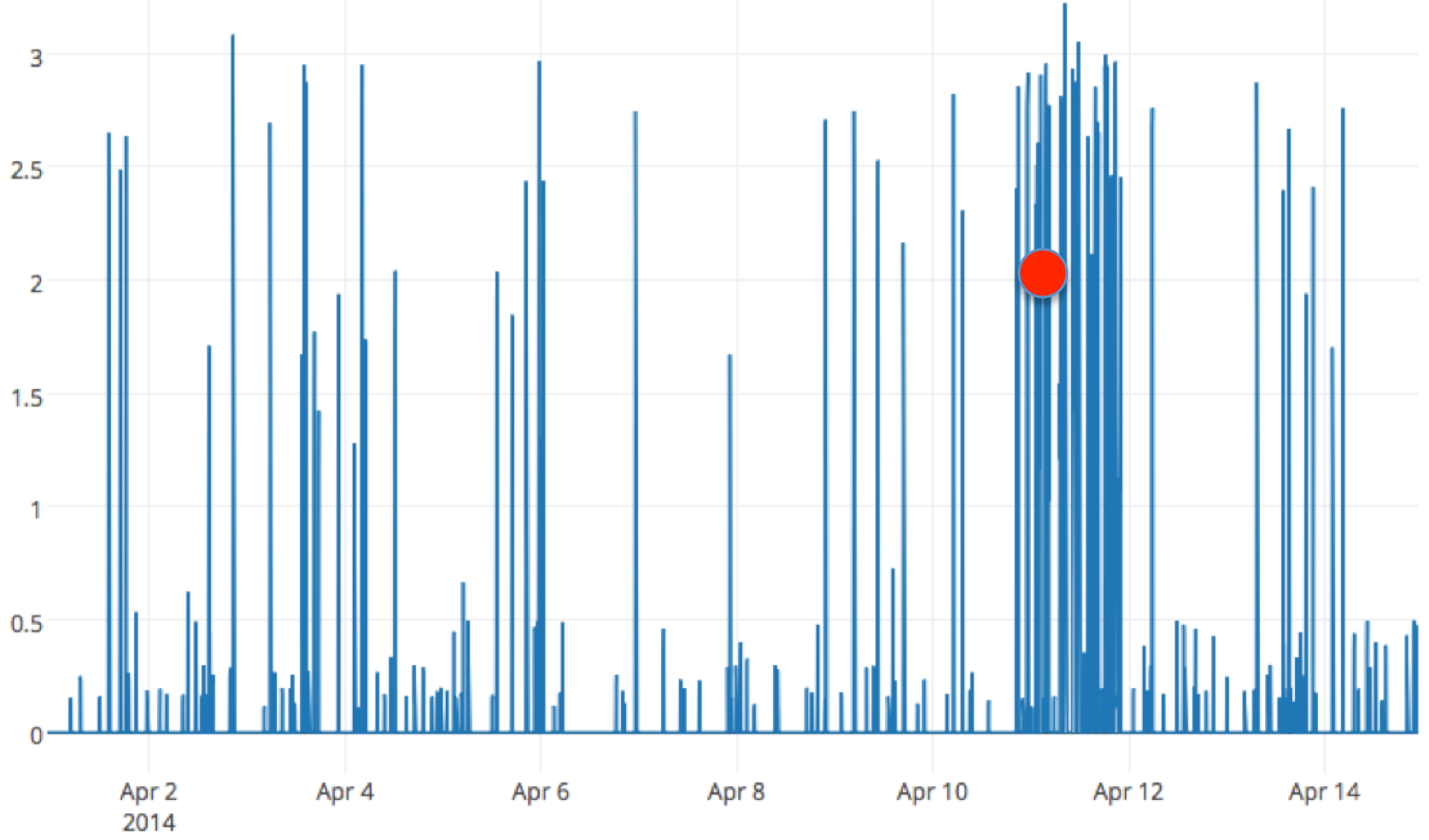
The raw anomaly score described above represents an instantaneous measure of the predictability of the current input stream. This works well for predictable scenarios but in many practical applications, the underlying system is inherently noisy and unpredictable. In these situations it is often the change in predictability that is indicative of anamolous behavior. As an example, consider Figure 4. This data shows the latency of a load balancer in serving HTTP requests on a production web site. Although the latency is generally low, it is not unusual to have occasional random jumps, and the corresponding spike in anomaly score. Thresholding the raw anomaly score directly would lead to many false positives. However, a sustained increase in the frequency of high latency requests, as shown in the second half of the figure, is unusual and thus reported as an anomaly.
To handle this class of scenarios, we introduce a second step. Rather than thresholding the raw score directly, we model the distribution of anomaly scores and use this distribution to check for the likelihood that the current state is anomalous. The anomaly likelihood is thus a metric defining how anomalous the current state is based on the prediction history of the HTM model. To compute the anomaly likelihood we maintain a window of the last raw anomaly scores. We model the distribution as a rolling normal distribution where the sample mean and variance are continuously updated from previous anomaly scores as follows:
| (3) |
| (4) |
We then compute a recent short term average of anomaly scores, and apply a threshold to the Gaussian tail probability (Q-function, (Karagiannidis & Lioumpas, 2007)) to decide whether or not to declare an anomaly222The Guassian tail probability is the probability that a Gaussian variable will obtain a value larger than standard deviations above the mean.. We define the anomaly likelihood as the complement of the tail probability:
| (5) |
where:
| (6) |
here is a window for a short term moving average, where . We threshold and report an anomaly if it is very close to :
| (7) |
It is important to note that this test is applied to the distribution of anomaly scores, not to the distribution of underlying metric values . As such, it is a measure of how well the model is able to predict, relative to the recent history. In clean predictable scenarios behaves similarly to . In these cases the distribution of scores will have very small variance and will be centered near . Any spike in will similarly lead to a corresponding spike in . However in scenarios with some inherent randomness or noise, the variance will be wider and the mean further from . A single spike in will not lead to a significant increase in but a series of spikes will. Interestingly, a scenario that goes from wildly random to completely predictable will also trigger an anomaly.
Since thresholding involves thresholding a tail probability, there is an inherent upper limit on the number of alerts. With very close to it would be unlikely to get alerts with probability much higher than . This also imposes an upper bound on the number of false positives. Under the assumption that anomalies themselves are also extremely rare, the hope is that the ratio of true positives to false positives is always in a healthy range (see Results below).
Although we use HTM as the underlying temporal model, the likelihood technique is not specific to HTMs. It could be used with any other algorithm that outputs a sparse code or scalar anomaly score. The overall quality of the detector will be dependent on the ability of the underlying model to represent the domain.
3.3 Combining Multiple Independent Models
Many industrial or complex environments contain a large number of sensory data streams. In theory, given sufficient resources, it is possible to create one large complex model with the entire vector stream as input. In practice, it is common to decompose a large system into a number of smaller models. It is easier to train smaller models because the complexity of training and inference grows much faster than linearly with the size of the input dimensionality (Bishop, 2006). Thus decomposing the solution into a set of smaller models may lead to improved accuracy and much faster performance. However, even with such a decomposition, it is important to compute a global measure that accumulates the results of individual models and indicates whether those portions of the system are in an unusual state. As an example, consider a datacenter running a production website. An automated alerting system might need to continually decide whether to generate an alarm and possibly wake up the on-call engineer.
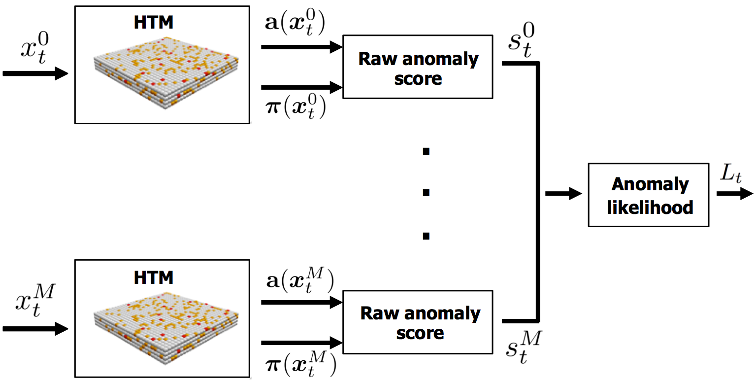
We assume the inputs representing the system are broken up into distinct models. Let be the input at time to the ’th model, and be the raw anomaly scores associated with each model. We wish to compute a global metric indicating the overall likelihood of an anomaly in the system (see Figure 5).
One possible approach is to estimate the joint distribution and apply a threshold to the tail probability. It can be challenging to model the joint distribution, particularly in a streaming context. If we further assume the models are independent, we could simplify and instead estimate:
| (8) |
Given this, a version of our anomaly likelihood can be computed as:
| (9) |
There is one flaw with the above methodology. In real-time dynamic scenarios, critical problems in one part of the system can often cascade to other areas. Thus there are often random temporal delays built in, which can in turn lead to different temporal delays between anomaly scores in the various models (Kim et al., 2013). For example, a situation where multiple unusual events occur close to one another in different models is far more unlikely and unusual than a single event in a single model. It is precisely these situations which are valuable to detect and capture in a complex system.
Ideally we would be able to estimate a joint distribution of anomaly scores that go back in time, i.e. . In theory this would capture all the dependencies, but this is even harder to estimate than the earlier joint probability. Alternatively, in situations where the system’s topology is relatively clear and under your control, it is possible to create an explicit graph of dependencies, monitor expected behavior between pairs of nodes, and detect anomalies with respect to those expectations. This technique has been shown to enable very precise determination of anomalies in websites where specific calls between services are monitored (Kim et al., 2013). However in most applications this technique is also impractical. It may be difficult to model the various dependencies and it is often infeasible to instrument arbitrary systems to create this graph.
We would like to have a system that is fast to compute, makes relatively few assumptions, and is adaptive. We propose a simple general purpose mechanism for handling multiple models by modifying Eq. (9) to incorporate a smooth temporal window. A windowing mechanism allows the system to incorporate spikes in likelihood that are close in time but not exactly coincident. Let be a Gaussian convolution kernel:
| (10) |
We apply this convolution to each individual model to obtain a final anomaly likelihood score333Since this is a real-time system with no look-ahead, the kernel only applies to time . As such we use a half-normal distribution as the kernel, hence the additional factor of 2.:
| (11) |
As before, we detect an anomaly if the combined anomaly likelihood is greater than a threshold . Eq. 11 represents a principled yet pragmatic approach for detecting anomalies in complex real time streaming applications444Due to numerical precision issues with products of probabilities, in our implementation we follow common practice and use summation of log probabilities.. As before, is an indirect measure, computed on top of the raw anomaly scores from each model. It reflects the underlying predictability of the models at a particular point in time and does not directly model the sensor measurements themselves.
3.4 Practical Considerations
There are three parameters in the single model scenario: , , and . is the duration for computing the distribution of anomaly scores. The system performance is not sensitive to as long as it is large enough to compute a reliable distribution. The number controls the short term average of anomaly scores. In all our experiments below, we use a generous value of and .
The parameter is perhaps the most important parameter. It controls how often anomalies are reported, and the balance between false positives and false negatives. In practice we have found that works well across a large range of domains. Intuitively, this should represent one false positive about once every 10,000 records.
The muliple model scenario introduces one additional parameter, the window width . This is somewhat domain dependent but due to the soft Gaussian convolution, the system is not extremely sensitive to this setting. In all our experiments below, .
Computational efficiency is important for real-time applications. In our implementation each model requires less than 10 milliseconds per input vector on a current high end laptop. A server based deployment running multiple models in parallel can run about 5,000 models on a high end server. This figure assumes that each input arrives once every 5 minutes (thus each of the 5,000 models needs to output one score every 5 minutes). As a service to the community, we have released the complete source code to the algorithms as well as the server application codebase as open source555Please see https://github.com/numenta, specifically the nupic and numenta-apps repositories..
4 Results
We first show examples from a deployed application that qualitatively demonstrates the behavior of our algorithm. We then show quantitative results on benchmark data.
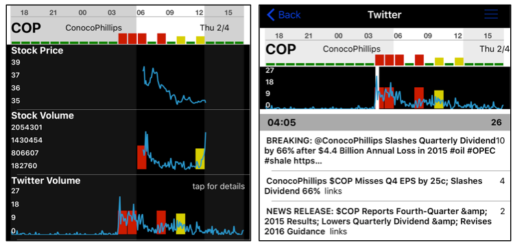
We have integrated our anomaly detection algorithm into a live real-time product. The application continuously monitors a large set of financial and social media metrics for a range of securities and alerts users in real time when significant anomalies occur. Figure 6 shows two screenshots from our application that demonstrate the value of real-time anomaly detection to end users. In this example, an anomaly in the volume of Twitter activity (related to a decrease in dividends) preceded a sharp drop in stock price. The Twitter anomaly occurred well before market opening. The underlying data streams are extremely noisy and many of the important anomalies are temporal in nature. Figure 7 shows raw data extracted from our application demonstrating one such anomaly. The figure plots stock trading volume for Facebook for a few hours. Each point represents average trading volume for a period of five minutes. It is normal to see a single spike in trading volume but it is extremely unusual to see two consecutive spikes. Two consecutive spikes therefore represents a temporal anomaly in this stream. The red dashed line indicates the point at which our algorithm detected the anomaly, i.e. the point in time where .
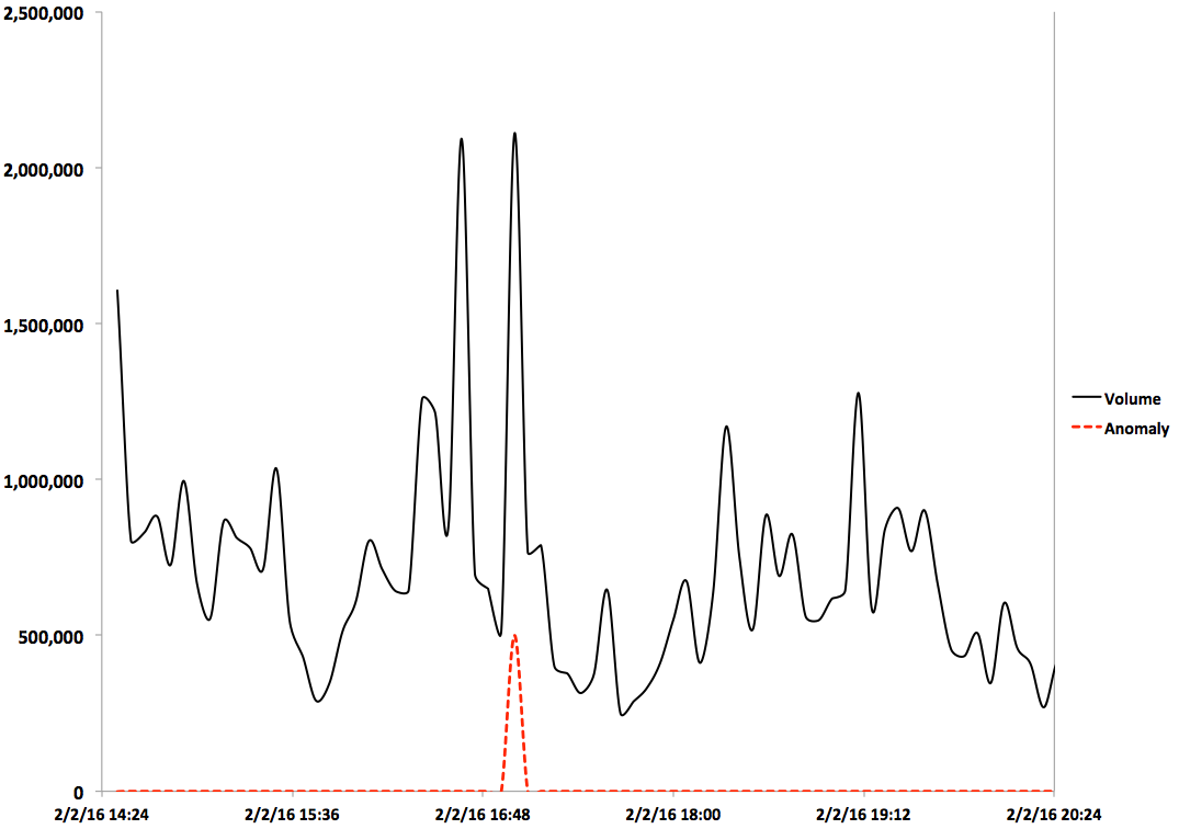
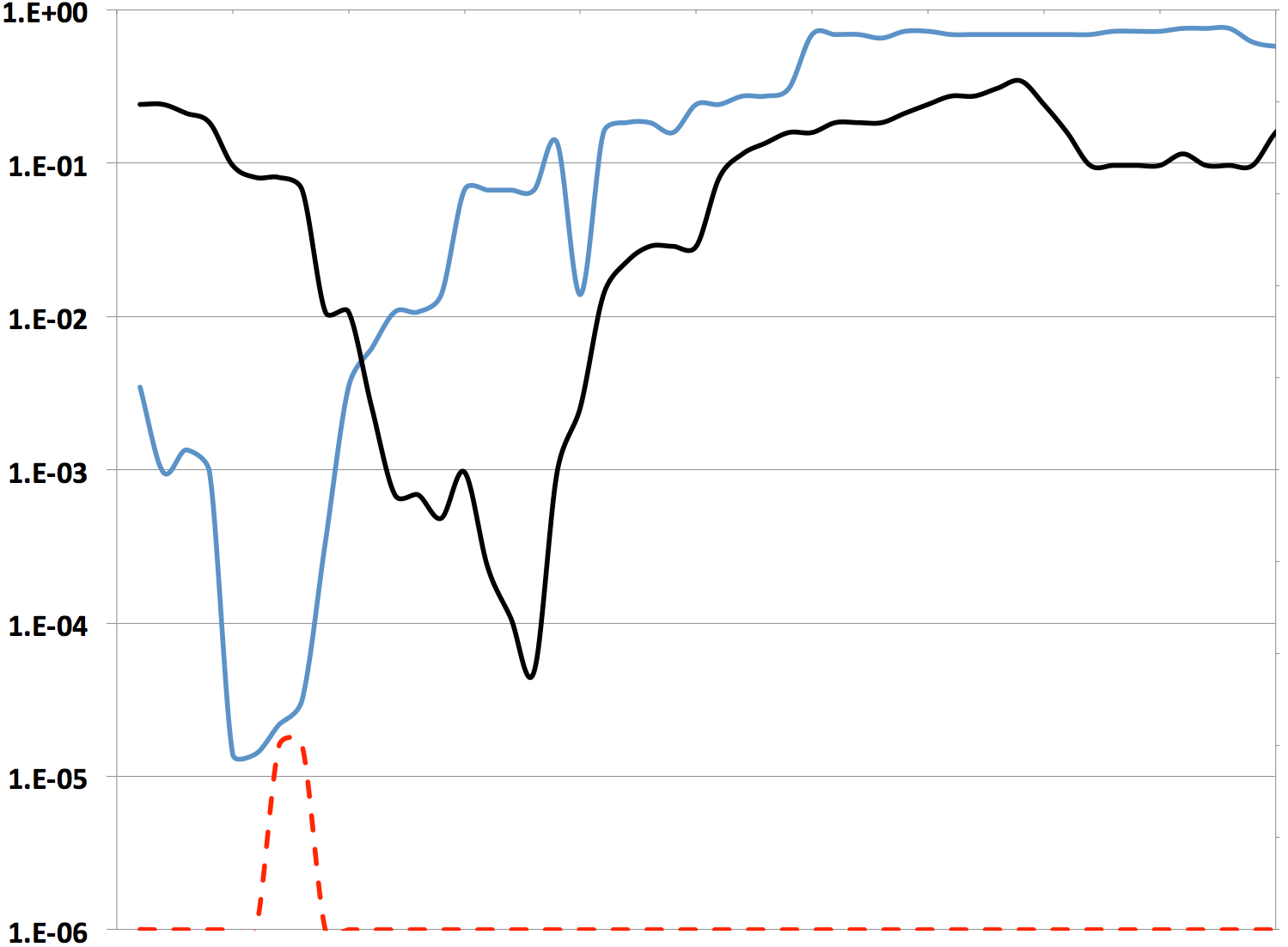
Figure 8 shows a more detailed example demonstrating the value of combining multiple metrics. The two solid lines indicate the Q-values in Eq (5) for two separate metrics related to Comcast shares. The lower the curve, the more likely it is that the underlying metric is anomalous. When looking at single models independently, an anomaly would only be detected if one of these values drops below . In this case no anomaly would be detected since neither one dips below that value. However, as shown by the drops, both metrics are behaving unusually. The red dashed line shows the result of detecting an anomaly based on our combined metric, Eq. (11). Because the blue curve is so close to , incorporating both metrics correctly flags an anomaly as soon as the black curve dips below . As can be appreciated from the chart, it is difficult to line up two metrics precisely, hence the value of the smooth temporal window.
4.1 Results on Real-World Benchmark Data
The above sections demonstrate qualitative results on individual data streams. In this section we provide quantitative benchmark results. NAB is a benchmark containing 58 streams with over 350,000 records of real-time streaming data taken from a variety of different applications (Lavin & Ahmad, 2015). The dataset is labeled with anomalies. The first 15% of each data file is reserved for auto-calibration. NAB also includes a window around each anomaly, and incorporates a time-sensitive scoring mechanism that favors early detection (as long as detections are within the anomaly windows). ”Application profiles” define the weighting for false positives and false negatives to illustrate scenarios where fewer missed detections or fewer erroneous detections are more valued. The benchmark requires models to use a single set of parameters across all streams to mimic automation in real-world deployments.
| Algorithm | NAB Score | Low FP | Low FN |
|---|---|---|---|
| Perfect | 100.0 | 100.0 | 100.0 |
| HTM | 65.3 | 58.6 | 69.4 |
| Twitter ADVec | 47.1 | 33.6 | 53.5 |
| Etsy Skyline | 35.7 | 27.1 | 44.5 |
| Bayes. Change Pt. | 17.7 | 3.2 | 32.2 |
| Sliding Threshold | 15.0 | 0.0 | 30.1 |
| Random | 11.0 | 1.2 | 19.5 |

We ran our HTM based anomaly detector on NAB. Table 1 contains our scores as well as scores for several other algorithms, including Etsy Skyline, Twitter AnomalyDetectionVec (ADVec), and a variant of Bayesian online change point detection (Adams & Mackay, 2007)666Please see the NAB repository at https://github.com/numenta/NAB for specific implementation and parameter tuning details.. We include the score for a “Perfect” detector, i.e. an idealized detector that detects every anomaly as early as possible and generates no false positives. We also include the scores for “sliding threshold” and “random” detectors as baselines for comparison. The HTM detector achieves the best overall score, followed by Twitter ADVec and Etsy Skyline. However, as can be seen by the performance of the Perfect detector, the benchmark is a challenging one with significant room for future improvements.
The NAB benchmark doesn’t measure an explicit ROC curve but includes two additional “application profiles” that tradeoff the weighting between false positives and false negatives. The “reward low FP” profile applies a higher cost to false positives. Conversely the “reward low FN” profile applies a higher cost to false negatives. The last two columns of Table 1 show our scores for those two profiles. Although there are individual variations (Twitter in particular improves significantly in the “reward low FN” column), our detector performs best overall indicating that it achieves a good tradeoff between false positives and false negatives.
A closer look at the errors illustrates some interesting situations that arise in real time applications. Figure 9(a) demonstrates the value of continuous learning. This file shows CPU usage on a production server over time and contains two anomalies. The first is a simple spike detected by all algorithms. The second is a sustained shift in the usage. Skyline and HTM both detect the change but then adapt to the new normal (with Skyline adapting quickest). Twitter ADVec however continues to generate anomalies for several days. Skyline scored highest on this stream.
Figure 9(b) and (c) demonstrate temporal anomalies and their importance in early detection. Figure 9(b) is an example demonstrating early detection. All three detectors detect the anomaly but HTM detects it three hours earlier due to a subtle shift in metric dynamics. Figure 9(c) shows a close up of the results for the machine temperature sensor data shown in Figure 1. The anomaly on the left is a somewhat subtle temporal anomaly where the temporal behavior is unusual but individual readings are within the expected range. This anomaly (which preceded the catastrophic failure on February 8) is only detected by HTM. All three detectors detect the anomaly on the right, although Skyline and HTM detect it earlier than ADVec. In this plot HTM and Skyline also each have a false positive.
We chose these examples because they illustrate common situations that occur in practice. Qualitatively we have found that temporal changes in behavior often precede a larger, easily detectable, shift. Temporal and sequence based anomaly detection techniques may be able to detect anomalies in streaming data before they are easily visible. We speculate that the early detection in Figure 9(b) is due to the temporal modeling in HTMs as the earlier shift is difficult to detect through purely spatial means. This provides hope that such algorithms can be used in production to provide early warning and perhaps help avoid problems far more reliably than spatial techniques.
Low scores for Bayesian change point detection are due to its strong assumptions regarding a Gaussian or Gamma distribution of data points. Real-world streaming data is messy and these assumptions do not hold in many applications. In data where it does hold (e.g. Figs 2, 9a) the algorithm works well but for most streams (e.g. Figs 1, 4) it does not. Indeed, it is this lack of any consistent distribution across streaming applications that led us to model the distribution of anomaly scores rather than the distribution of metric values.
From the standpoint of computational efficiency, on the first author’s laptop, it takes 48 minutes to run NAB’s complete dataset of 365,558 records. This represents an average of 8 milliseconds per record.
5 Discussion
With the increase in connected real-time sensors, the detection of anomalies in streaming data is becoming increasingly important. The use cases cut across a large number of industries; anomaly detection might represent the most significant near-term application for machine learning in IoT.
In this paper we have discussed a novel anomaly detection algorithm for real-time streaming applications. Based on HTMs, the algorithm is capable of detecting spatial and temporal anomalies in predictable and noisy domains. A probabilistic formulation allows the user to control the rate of false positives, an important consideration in many applications. We have discussed an extension to large systems with multiple independent models that incorporate temporal windows.
Our results show that the algorithm can achieve best in class results on a benchmark of real world data sources. Our system is practical in that it is computationally efficient, automatically adapts to changing statistics, and requires little to no parameter tuning. It is currently in use in commercial applications, and the complete source code to the algorithm is available as open source software777Please see http://numenta.com/nab.
There are a number of possible extensions to the algorithm. The error analysis from NAB indicates that the errors from our algorithm are not necessarily correlated with errors from the other two algorithms. As such an ensemble based approach might provide a significant increase in accuracy. The assumption of a Gaussian distribution for anomaly scores is not always correct. Exploring other distributions represents another possible extension that could potentially improve the results.
Acknowledgements
We thank Alex Lavin, Yuwei Cui, and Jeff Hawkins for many helpful comments and suggestions.
References
- Adams & Mackay (2007) Adams, Ryan Prescott and Mackay, David J. C. Bayesian Online Changepoint Detection. arXiv.org, pp. 7, 2007. doi: arXiv:0710.3742v1. URL http://arxiv.org/abs/0710.3742.
- Ahmad & Hawkins (2016) Ahmad, Subutai and Hawkins, Jeff. How do neurons operate on sparse distributed representations? A mathematical theory of sparsity, neurons and active dendrites. pp. arXiv:1601.00720 [q–bio.NC], jan 2016. URL http://arxiv.org/abs/1601.00720.
- Basseville & Nikiforov (1993) Basseville, M and Nikiforov, I V. Detection of Abrupt Changes, volume 2. 1993.
- Bianco et al. (2001) Bianco, A. M., García Ben, M., Martínez, E. J., and Yohai, V. J. Outlier detection in regression models with ARIMA errors using robust estimates. Journal of Forecasting, 20(8):565–579, 2001.
- Bishop (2006) Bishop, Christopher M. Pattern Recognition and Machine Learning, volume 4. Springer, 2006. ISBN 9780387310732.
- Bloom (1970) Bloom, Burton H. Space/time trade-offs in hash coding with allowable errors, 1970. ISSN 00010782.
- Chandola et al. (2008) Chandola, V., Mithal, V., and Kumar, V. Comparative Evaluation of Anomaly Detection Techniques for Sequence Data. 2008 Eighth IEEE International Conference on Data Mining, pp. 743–748, 2008. ISSN 1550-4786. doi: 10.1109/ICDM.2008.151.
- Chandola et al. (2009) Chandola, Varun, Banerjee, A, and Kumar, V. Anomaly detection: A survey. ACM Computing Surveys (CSUR), (September):1–72, 2009.
- Cui et al. (2015) Cui, Yuwei, Surpur, Chetan, Ahmad, Subutai, and Hawkins, Jeff. Continuous online sequence learning with an unsupervised neural network model. pp. arXiv:1512.05463 [cs.NE], 2015. URL http://arxiv.org/abs/1512.05463.
- Fox (1972) Fox, A J. Outliers in time series. Journal of the Royal Statistical Society, Series B (Methodological), 34(3):350–363, 1972. ISSN 00359246.
- Görnitz et al. (2013) Görnitz, Nico, Kloft, Marius, Rieck, Konrad, and Brefeld, Ulf. Toward supervised anomaly detection. Journal of Artificial Intelligence Research, 46:235–262, 2013. ISSN 10769757. doi: 10.1613/jair.3623.
- Hawkins & Ahmad (2016) Hawkins, Jeff and Ahmad, Subutai. Why Neurons Have Thousands of Synapses, a Theory of Sequence Memory in Neocortex. Frontiers in Neural Circuits, 10(23):1–13, mar 2016. ISSN 1662-5110. doi: 10.3389/fncir.2016.00023. URL http://journal.frontiersin.org/article/10.3389/fncir.2016.00023/abstract.
- Hodge & Austin (2004) Hodge, Victoria J. and Austin, Jim. A survey of outlier detection methodologies, 2004. ISSN 02692821.
- Hyndman & Khandakar (2008) Hyndman, Rob J and Khandakar, Yeasmin. Automatic time series forecasting : the forecast package for R Automatic time series forecasting : the forecast package for R. Journal Of Statistical Software, 27(3):1–22, 2008.
- Karagiannidis & Lioumpas (2007) Karagiannidis, George K. and Lioumpas, Athanaszsios S. An improved approximation for the Gaussian Q-function. IEEE Communications Letters, 11(8):644–646, 2007.
- Kejariwal (2015) Kejariwal, Arun. Twitter Engineering: Introducing practical and robust anomaly detection in a time series [Online blog], 2015. URL http://bit.ly/1xBbX0Z.
- Keogh et al. (2005) Keogh, Eamonn, Lin, Jessica, and Fu, Ada. HOT SAX: Efficiently finding the most unusual time series subsequence. In Proceedings - IEEE International Conference on Data Mining, ICDM, pp. 226–233, 2005. ISBN 0769522785. doi: 10.1109/ICDM.2005.79.
- Kim et al. (2013) Kim, Myunghwan, Sumbaly, Roshan, and Shah, Sam. Root cause detection in a service-oriented architecture. ACM International Conference on Measurement and Modeling of Computer Systems (SIGMETRICS ’13), pp. 93, 2013. doi: 10.1145/2465529.2465753.
- Klerx et al. (2014) Klerx, Timo, Anderka, Maik, Buning, Hans Kleine, and Priesterjahn, Steffen. Model-Based Anomaly Detection for Discrete Event Systems. In 2014 IEEE 26th International Conference on Tools with Artificial Intelligence, pp. 665–672. IEEE, nov 2014. ISBN 978-1-4799-6572-4. doi: 10.1109/ICTAI.2014.105.
- Laptev et al. (2015) Laptev, Nikolay, Amizadeh, Saeed, and Flint, Ian. Generic and Scalable Framework for Automated Time-series Anomaly Detection. In Proceedings of the 21th ACM SIGKDD International Conference on Knowledge Discovery and Data Mining, pp. 1939–1947. ACM, 2015.
- Lavin & Ahmad (2015) Lavin, Alexander and Ahmad, Subutai. Evaluating Real-time Anomaly Detection Algorithms – the Numenta Anomaly Benchmark. In 14th International Conference on Machine Learning and Applications (IEEE ICMLA’15), Miami, Florida, 2015. IEEE. doi: 10.1109/ICMLA.2015.141.
- Lee et al. (2013) Lee, Eun Kyung, Viswanathan, Hariharasudhan, and Pompili, Dario. Model-based thermal anomaly detection in cloud datacenters. Proceedings - IEEE International Conference on Distributed Computing in Sensor Systems, DCoSS 2013, pp. 191–198, 2013. doi: 10.1109/DCOSS.2013.8.
- Padilla et al. (2013) Padilla, Daniel E., Brinkworth, Russell, and McDonnell, Mark D. Performance of a hierarchical temporal memory network in noisy sequence learning. In 2013 IEEE International Conference on Computational Intelligence and Cybernetics (CYBERNETICSCOM), pp. 45–51. IEEE, dec 2013. ISBN 978-1-4673-6053-1. doi: 10.1109/CyberneticsCom.2013.6865779.
- Rebbapragada et al. (2009) Rebbapragada, Umaa, Protopapas, Pavlos, Brodley, Carla E., and Alcock, Charles. Finding anomalous periodic time series : An application to catalogs of periodic variable stars. Machine Learning, 74(3):281–313, 2009. ISSN 08856125. doi: 10.1007/s10994-008-5093-3.
- Rozado et al. (2012) Rozado, David, Rodriguez, Francisco B., and Varona, Pablo. Extending the bioinspired hierarchical temporal memory paradigm for sign language recognition. Neurocomputing, 79:75–86, mar 2012. ISSN 09252312. doi: 10.1016/j.neucom.2011.10.005.
- Simon & Rinehart (2015) Simon, Donald L and Rinehart, Aidan W. A Model-Based Anomaly Detection Approach for Analyzing Streaming Aircraft Engine Measurement Data. Technical Report 2015-218454, NASA, 2015.
- Stanway (2013) Stanway, A. Etsy Skyline, 2013. URL https://github.com/etsy/skyline.
- Szmit & Szmit (2012) Szmit, MacIej and Szmit, Anna. Usage of modified holt-winters method in the anomaly detection of network traffic: Case studies. Journal of Computer Networks and Communications, 2012, 2012. ISSN 20907141. doi: 10.1155/2012/192913.
- Tartakovsky et al. (2013) Tartakovsky, Alexander G., Polunchenko, Aleksey S., and Sokolov, Grigory. Efficient Computer Network Anomaly Detection by Changepoint Detection Methods. IEEE Journal of Selected Topics in Signal Processing, 7(1):4–11, feb 2013. ISSN 1932-4553. doi: 10.1109/JSTSP.2012.2233713. URL http://ieeexplore.ieee.org/lpdocs/epic03/wrapper.htm?arnumber=6380529.
- Tsay (2000) Tsay, R. S. Outliers in multivariate time series. Biometrika, 87(4):789–804, dec 2000. ISSN 0006-3444. doi: 10.1093/biomet/87.4.789.