Is there substructure around M87?

Abstract

We present a general method to identify infalling substructure in discrete datasets with position and line-of-sight velocity data. We exploit the fact that galaxies falling onto a brightest cluster galaxy (BCG) in a virialised cluster, or dwarf satellites falling onto a central galaxy like the Milky Way, follow nearly radial orbits. If the orbits are exactly radial, we show how to find the probability distribution for a satellite’s energy, given a tracer density for the satellite population, by solving an Abel integral equation. This is an extension of Eddington (1916)’s classical formula for the isotropic distribution function. When applied to a system of galaxies, clustering in energy space can then be quantified using the Kullback-Leibler divergence, and groups of objects can be identified which, though separated in the sky, may be falling in on the same orbit. This method is tested using mock data and applied to the satellite galaxy population around M87, the BCG in Virgo, and a number of associations are found which may represent infalling galaxy groups.

1 Introduction

In the hierarchical model of galaxy formation, elliptical galaxies and the stellar haloes of spiral galaxies are built up gradually by prolonged periods of accretion. In this picture, early-type galaxies form during an early phase of dissipational star formation fed by gas-rich mergers, creating compact cores, while their subsequent evolution is mainly driven by abundant minor mergers, feeding the outer regions of the galaxy and bringing them onto the local size-mass relation (e.g. Shen et al., 2003; Naab et al., 2009; Hopkins et al., 2010).

This phenomenon is even more important in clusters, where the brightest cluster galaxies (BCGs) that reside in their centres are thought to have acquired the majority of their stars through the accumulation and subsequent destruction of satellite galaxies (Laporte et al., 2013; Cooper et al., 2015). BCGs have haloes that are embedded in the intracluster light, and it is not obvious whether a useful distinction between the halo and the intra-cluster medium is even possible (Gonzalez et al., 2005); the disruption of satellite galaxies as they are funnelled by dynamical friction from the intra-cluster medium onto the central BCG then creates an extensive envelope. Indeed, it is possible that the progenitors of today’s BCGs are the extremely compact ‘red nuggets’ that have been observed at redshifts $z\sim 2$ (e.g. Trujillo et al., 2007; van Dokkum et al., 2008). The evolution of the BCG is therefore dominated by the addition of stars and globular clusters that have formed outside the BCG itself.

In the Local Group, a much lower-mass example compared to galaxy clusters, the biggest members show convincing evidence of a structured satellite galaxy population. For instance, the Large Magellanic Cloud, together with its satellites, may be part of an extended group that is on its first infall onto the Milky Way (Koposov et al., 2015), while M31 seemingly has an extended thin disk of satellites (Ibata et al., 2013) that may be the result of group infall and accretion (e.g. Bowden et al., 2014). In these systems, detailed searches for substructure are made possible by the high-quality six-dimensional phase-space data that are available for individual stars (e.g. Xue et al., 2011).

Given these findings, the extreme densities found in cluster environments make it very likely that the outer parts of BCGs are also permeated with radially infalling satellite groups. However, substructure identification in these much more distant systems cannot be carried out using the same methods as in the Local Group as it is not possible to resolve individual stars, and bright stellar proxies such as globular clusters, planetary nebulae and satellite galaxies must be used instead. Another difficulty is that these studies must be carried out using projected data, as only three of the full six-dimensional phase space coordinates are usually available – namely, position on the sky and line-of-sight velocity – and this gives rise to much larger uncertainty. Nevertheless, a number of recent studies have used globular cluster kinematics to find evidence for recent accretion events (e.g. Côté et al., 2003; Schuberth et al., 2010; Romanowsky et al., 2012; Longobardi et al., 2015), while searches for apparent photometric disturbances such as shells and tidal tails have also made strong cases for recent and ongoing accretion (Tal et al., 2009). Extended sheets or pancakes of satellite galaxies have also been tentatively identified in the outskirts of clusters (Falco et al., 2013).

Here, we introduce a new method to identify members of the same infalling satellite galaxy group in a cluster, using only projected galactocentric distances and line-of-sight velocities. We argue that, in the outer parts of clusters, galaxies are falling in on almost radial orbits. This suggests an appealing simple ansatz, namely that the distribution function (DF) is

$$F\propto\delta(v_{\theta})\delta(v_{\phi})f(E)$$ (1)

where $v_{r},v_{\theta},v_{\phi}$ are velocity components resolved with respect to the spherical polar coordinates and $E$ is the energy. In Section 2, we show that this leads to an Abel inversion, which can be performed exactly. In other words, for any tracer density of objects, a DF of this form can be found, although – as always – we must check for positive definiteness a posteriori. As an application, Section 3 applies the method to the dataset of satellite galaxies around M87, one of the most massive galaxies in the local universe. This giant E0 elliptical resides at the centre of the Virgo cluster, and its environment has been catalogued extensively by Binggeli et al. (1985) and Kim et al. (2014). Here, we use the carefully-selected subsample of Virgo galaxies considered to be certain M87 satellites, compiled by Oldham & Auger (2016b), and identify possible substructures by looking for objects which are clustered in energy space, and hence falling onto M87 on the same orbital path but with different phases. Finally, we summarise in Section 4 and consider possible extensions, applications and future prospects for our method.

2 Radial Orbit Models

We consider spherical densities of tracer satellites all moving on exactly radial orbits. The DF must depend on the integrals of motion (Jeans theorem). These are binding energy $E$ and square of the angular momentum $L^{2}$ given by

$$E = \psi(r)-\frac{1}{2}(v_{r}^{2}+v_{T}^{2})$$

$$L^{2} = r^{2}v_{T}^{2}$$ (2)

where $v_{r}$ and $v_{T}$ are the radial and tangential velocity components judged from the centre of the cluster. The gravitational (relative) potential $\psi$ is unknown, and we wish to solve for properties of the potential given the kinematics of the tracers.

Velocity anisotropy is usually characterised by the anisotropy parameter $\beta=1-\langle v_{\rm T}^{2}\rangle/\langle v_{r}^{2}\rangle$, where angled brackets denote averages over the velocity distribution. Models with purely radial orbits, such as the ones presented in this paper, have $\beta=1$ everywhere. While this assumption is clearly an idealisation, many simulations of hierarchical formation do produce very strongly radially anisotropic structures – for instance, the galaxy haloes formed by Bullock & Johnston (2005) have $\beta\approx 0.8$, as can be clearly seen in Figure 8 of Williams & Evans (2015). Similarly, simulated galaxy clusters have been found to have strongly radial anisotropy parameters $\beta\approx 0.7$ in the outer regions, as in Figure 3.2 of Sarli et al. (2014). However, there is considerable cosmic variance and values $\beta\approx 0.3-0.5$ for clusters are also present in the literature (see e.g., Cuesta et al., 2008; Wojtak et al., 2008; Prada et al., 2012). Therefore, the assumption we make here is a simplification that applies to some, but by no means all, clusters.

2.1 The general case

For any tracer density $\nu$, the integral equation for the DF $F(E,L^{2})=F_{E}(E)\delta(L^{2})$ is of Abel form and can be inverted in a similar manner to Eddington (1916)’s classical work to give

$$F_{E}(E)={\sqrt{2}\over\pi^{2}}{d\over dE}\int_{0}^{E}{d\psi\over(E-\psi)^{1/2}}r^{2}\nu,$$ (3)

where $r^{2}\nu$ is regarded as a function of $\psi$ via the inversion of $\psi(r)$. This is the general solution for the DF of any radial orbit model. Note that the well-known Osipkov-Merritt models (see e.g., Binney & Tremaine, 1987) attain $\beta=1$ or extreme radial anisotropy at large distances, and so are closely related to our models.

The problem is straightforward if the function $F_{E}$ is a power-law, so that the DF has the form

$$F(E,L^{2})=\begin{cases}F_{0}\delta(L^{2})(E-E_{0})^{-p}&E\geq E_{0}\cr 0&E<E_{0},\end{cases}$$ (4)

where $F_{0}$ is a normalisation constant. The model has a finite edge $r_{\rm t}$ at which $\psi(r_{\rm t})=E_{0}$. The density is obtained by integrating over velocity space as

$$\nu(r)={\pi^{{\frac{3}{2}}}\Gamma(1-p)\over\sqrt{2}\Gamma({\frac{3}{2}}-p)}{F_{0}\over r^{2}(\psi-E_{0})^{p\!-\!{\frac{1}{2}}}},$$ (5)

with $p<1$. By integrating along the line of sight, we obtain the surface density $\Sigma(R)$ as:

$$\Sigma(R)={\sqrt{2}\pi^{{\frac{3}{2}}}\Gamma(1\!-\!p)F_{0}\over\Gamma({\frac{3}{2}}\!-\!p)}\int_{R}^{r_{\rm t}}{dr\over r(r^{2}\!-\!R^{2})^{{\frac{1}{2}}}(\psi\!-\!E_{0})^{p\!-\!{\frac{1}{2}}}}.$$ (6)

The intrinsic velocity dispersions generated by this model are

$$\langle v_{r}^{2}\rangle={2\over 3-2p}\left(\psi-E_{0}\right),\qquad\langle v_{\theta}^{2}\rangle=\langle v_{\phi}^{2}\rangle=0.$$ (7)

There is no dispersion in the angular velocities, as the satellite galaxies all move on radial orbits. The square of the radial velocity dispersion is proportional to the gravitational potential.

The data on any satellite comprise projected positions $R$ and line-of-sight velocities $v_{\rm los}$. Let ${\cal P}$ be shorthand for the parameters of the model. Using the product rule for probabilities, we have:

$$P(v_{\rm los},R|{\cal P})=P(v_{\rm los}|R,{\cal P})P(R|{\cal P}).$$ (8)

Here, $P(R|{\cal P})$ is the probability of finding a satellite galaxy at projected position $R$, which is just $2\pi R\Sigma(R)$, modulated by the selection function $S(R)$ of the survey. The probability distribution of line-of-sight velocity $v_{\rm los}$ at any position is

$$P(v_{\rm los}|R,{\cal P})={2\pi F_{0}\over\Sigma(R)}J(v_{\rm los},R),$$ (9)

with

$$J(v_{\rm los},R)=\int^{r_{\rm t}}_{{r_{-}}}{dr\over[(r^{2}\!-\!R^{2})(\psi\!-\!E_{0})\!-\!\frac{1}{2}v^{2}_{\rm los}r^{2}]^{p}(r^{2}\!-\!R^{2})^{1\!-\!p}}.$$ (10)

Here, ${r_{-}}$ is the smallest positive root for $x$ of

$$(x^{2}-R^{2})(\psi(x)-E_{0})-\frac{1}{2}v^{2}_{\rm los}x^{2}=0.$$ (11)

The physical significance of ${r_{-}}$ is that it is the minimum three-dimensional position at which we can find a radial orbit whose velocity projected along the line of sight is $v_{\rm los}$.

Given a set of $N$ satellite galaxies with projected positions $R_{j}$ and line of sight velocities $v_{{\rm los},j}$, the logarithm of the likelihood is then

$$\log L=\sum_{j=1}^{N}\log P(v_{{\rm los},j},R_{j}|{\cal P}),$$ (12)

whose maximum needs to be found via a grid search to identify the best model parameters ${\cal P}$. If the spatial selection function $S(R)$ is not known, we can still make progress by taking the likelihood as

$$\log L\approx\sum_{j=1}^{N}\log P(v_{{\rm los},j}|R_{j},{\cal P}),$$ (13)

which is tantamount to assuming that the surface density falls approximately like $R^{-1}$ and makes only a modest contribution to the likelihood. We check the validity of this assumption a posteriori.

2.2 Power-law tracers

So far, we have described the method for an arbitrary spherical potential. Now, let us consider a specific case which can be applied to real datasets. We assume that the potential $\psi$ behaves like a power law

$$\psi=\psi_{0}\left({r_{0}\over r}\right)^{\alpha},$$ (14)

so that (assuming $r_{\rm t}\rightarrow\infty$ so $E_{0}\rightarrow 0$)

$$\nu(r)=N_{0}\left({r_{0}\over r}\right)^{\gamma},$$ (15)

where the normalisation constant $N_{0}$ is given in Appendix A. We have put $p=\frac{(2-\gamma)}{\alpha}+\frac{1}{2}$, so that the absolute value of the logarithmic gradient of the potential is $\alpha$ and that of the density is $\gamma$.

The observables – the surface density and the line-of-sight velocity dispersions – are also power laws given by

$$\Sigma(R) = S_{0}\left({r_{0}\over R}\right)^{\gamma-1},$$

$$\langle v_{\rm los}^{2}\rangle = v_{0}^{2}\left({r_{0}\over R}\right)^{\alpha},$$ (16)

where again the normalisation constants $S_{0}$ and $v_{0}$ are relegated to the Appendix. Our model therefore describes a population of satellite galaxies whose density and velocity dispersion profiles are power laws to at least a reasonable approximation. This is reasonable given that satellite galaxies mainly reside in the outer parts. For the same reason, we also do not worry about the singularity of the power-laws at $r=0$.

In this model, the distribution of line-of-sight velocities (the line profile) is

$$P(v_{\rm los}|R,{\cal P})={2\pi F_{0}\over\Sigma(R)}J(v_{\rm los},R),$$ (17)

with

$$J=\int^{r_{\rm t}}_{{r_{-}}}{r^{2-\gamma+\alpha/2}dr\over[\psi_{0}r_{0}^{\alpha}(r^{2}-R^{2})-\frac{1}{2}v^{2}_{\rm los}r^{\alpha+2}]^{p}(r^{2}-R^{2})^{1-p}}.$$ (18)

As before, ${r_{-}}$ is the root of

$$(x^{2}-R^{2})\psi_{0}r_{0}^{\alpha}-\frac{1}{2}v^{2}_{\rm los}x^{\alpha+2}=0.$$ (19)

This enables us to construct the logarithm of the likelihood according to Equation (13), and therefore find the best fit of our model to data.

As an aside, we briefly note that the case $p={\frac{1}{2}}$ is a singular limit and eq. (5) becomes independent of the potential. The model is then the exact solution discovered by Fridman & Polyachenko (1984) and reported in Binney & Tremaine (1987). Choosing $F_{0}=\sqrt{2}C/\pi^{2}$, the model then has a density given by

$$\nu(r)=\begin{cases}{\displaystyle C\over\displaystyle r^{2}}&r<r_{\rm t}\\ 0&r>r_{\rm t}.\end{cases}$$ (20)

Unlike the models described earlier in this Section, this DF solves Equation (5 in a self-consistent way, such that the potential and density are related via Poisson’s equation. As is well-known, such self-consistent models are subject to the radial orbit instability; however, we emphasise that this does not apply to our models in which the distribution function describes a tracer population and so stability is not compromised.

Figure 1: A map of the satellite galaxies, colour-coded by line-of-sight velocity. M87 is shown by a black star.

3 Case Study: M87

3.1 Data

We demonstrate the working of this method by applying it to the population of satellite galaxies belonging to M87, the BCG in the Virgo cluster, located at redshift $z=0.004$ or a distance $D_{L}=16.5$ Mpc (Mei et al., 2007). Though Virgo is a relatively poor cluster compared to others (e.g. Coma), its proximity to us means it is perhaps the best studied: Binggeli et al. (1985) were the first to compile an extensive catalogue of possible cluster members, comprising 2096 galaxies within an area of $\sim 140$ deg², including velocities for 572 objects, and classifying 1227 galaxies as certain cluster members. More recently, Kim et al. (2014) presented an Extended Virgo Cluster Catalogue (EVCC) based on the Sloan Digital Sky Survey (SDSS) Data Release 7, increasing the area coverage by a factor of 5. The EVCC includes 1589 cluster candidates – 1324 of which have velocities measured from the SDSS spectra, with the remainder having velocity measurements taken from Ned Wright’s Extragalactic Database (NED) – with each classified as a certain or possible cluster member according to morphological and spectroscopic criteria. However, Virgo has a somewhat complex environment comprising a number of sub-clumps, with two main ‘clouds’ – the A cloud, centred on M87 and the B cloud, centred on M49, both at similar line-of-sight distances – along with a number of smaller structures, such as the W cloud, which is located slightly further away at $D_{L}\sim 23$ Mpc. This means that, to select a sample of galaxies that are associated dynamically with M87, it is not sufficient to simply take all confirmed cluster members: care must be taken to separate satellites belonging to the different structures, each of which has its own massive central object in whose potential the galaxies can be taken to move.

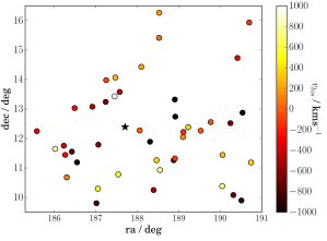
We therefore use the (significantly smaller) subset of satellites compiled in Oldham & Auger (2016b). While the selection criteria were fully explained in that paper, we briefly summarise them here: objects classified as certain cluster members in Kim et al. (2014) were cross-correlated with the distance modulus catalogue of Blakeslee et al. (2009) and removed from the sample if $D_{L}>20$ Mpc, to avoid contamination with the smaller, more distant substructures. While this step has a dramatic effect on the number of objects in the sample, it is important because it is impossible to tell from redshift measurements alone whether an object is at the desired distance or instead has a peculiar velocity which only makes it appear to be. Objects with declination angles $<9$ degrees were further removed to avoid contamination from the B cloud. Here, we apply a further cut in projected radius $R<800$ kpc, beyond which the potential from the other subclumps may be having a non-negligible effect on the dynamics. This leaves a catalogue of 50 satellites ranging from 248 kpc to 794 kpc from the centre of M87, as shown in Figure 1. We note that while the EVCC does not provide uncertainties on the velocity measurements, it does provide a comparison between SDSS and NED velocities for the 498 objects having measurements in both, and indicates a mean difference of $\Delta v=2.6$ kms^-1. We therefore assume all objects to have velocity uncertainties comparable to the typical uncertainty in the SDSS measurements, which we conservatively take to be 4 %. We also note that, since the sample in Kim et al. (2014) was selected spectroscopically, its distribution may not be representative of the underlying population – it may, for example, be missing the faintest galaxies – and that further, as we have applied additional rigorous cuts to eliminate contaminants, our sample is not complete. Nevertheless, we are able to make progress under the (not unreasonable assumption) that our sample is a close representation of the parent population.

Figure 2: The binned surface density of satellite galaxies (left) and the binned velocity dispersion profile (right), with the fit overplotted. The number of objects per bin is small (typically $\sim 5$). The deviation from the fit at the largest radii may be due to small-number statistics, or alternatively may be a sign of the limitations of our model.

3.2 Implementation: the DF

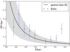
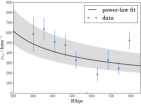
To fit to the observed line-of-sight velocities and projected distances for our sample of Virgo cluster galaxies, we carry out a grid search for the maximum-likelihood parameters $\psi_{0}$, $\alpha$ and $\gamma$ of the potential and density profiles, and account for uncertainties on the parameters due to uncertainties in the data by Monte-Carlo sampling – though we note that the projected positions $R$ have negligible uncertainty. We also allow for the uncertainty due to the curvature of the likelihood surface. The parameters are summarised in Table 1, together with 1$\sigma$ uncertainties. Figure 2 then shows the binned surface density and line-of-sight velocity dispersion, with our fitted profiles overplotted. This suggests the model is an encouraging match to the data and validates the assumptions made in our approach. We can also perform the test of assuming instead a constant selection function and fully incorporating the spatial information on the satellite galaxies in the likelihood. This changes the inference on both $\alpha$ and $\gamma$ by $\sim 0.1$, which is consistent with our current uncertainty.

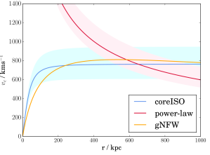
To test our inference, we compute the circular velocity profile predicted by our model and compare it with those inferred in Oldham & Auger (2016b), in which a more extensive dataset was used (encompassing stars and globular clusters in addition to the satellite galaxy population). In that study, models with stars and globular clusters moving on both isotropic and anisotropic orbits were considered, while in all cases, the anisotropy of the satellite population was calibrated using simulations and taken to be $\beta=0.3$: here, then, for simplicity, we compare with the isotropic case. Figure 3 shows the comparison: due to the distribution of the satellite galaxies, we expect to be constraining the potential most strongly at large radii. We see that, while the large-radius circular velocity profiles are comparable, we ultimately predict a lower circular velocity than in the isotropic models of Oldham & Auger (2016b); this can be clearly understood in terms of our very different assumptions about the anisotropy of the satellites, with the models considered here assuming totally radial infall as opposed to the much milder $\beta=0.3$ used in the Oldham & Auger (2016b) analysis.

$\log(\psi_{0})$	$\alpha$	$\gamma$	$\log(F_{0})$
$8.89\pm 0.07$	$1.13\pm 0.10$	$2.41\pm 0.13$	$-2.59\pm 0.07$

Table 1: Maximum-likelihood values for the potential normalisation $\psi_{0}$ and power-law index $\alpha$, the density power-law index $\gamma$ and the normalisation of the DF $F_{0}$, along with uncertainties.

Figure 3: A comparison of the circular velocity curves predicted by this model and the (cored isothermal and generalised NFW) models of Oldham & Auger (2016b). The deviation at small radii is mainly due to the fact that the majority of our satellite galaxies are at larger radii, meaning we cannot expect to constrain the potential there: also, we the power-law potential that we consider here is a simpler and more rigid model than in Oldham & Auger (2016b). On the other hand, the profiles agree quite well at large radii, with the potential inferred in this study slightly lower due to our assumption of complete radial anisotropy.

3.3 Implementation: clustering

Given our inferred potential and density parameters, we search for clustering in energy among the satellite population using the Kullbeck-Leibler divergence $D_{kl}$ (Kullback & Leibler, 1951). Recently, this has been used with success by Sanderson et al. (2015) to infer the gravitational potential of the Milky Way, and more generally is a good way of quantifying the difference between two distributions or probability distributions because of its natural interpretation in terms of probabilistic inference. Also known as the relative entropy, the $D_{kl}$ from $p(x)$ to $q(x)$ is given by

$$D_{kl}(p:q)=\int p(x)\log\frac{p(x)}{q(x)}dx,$$ (21)

which, following Sanderson et al. (2015), can also be written

$$D_{kl}(p:q) =\int p(x)\log p(x)dx-\int p(x)\log q(x)dx$$ (22)

$$=<\log L(H_{p}|x)>_{p}-<\log L(H_{q}|x)>_{p},$$

for logarithmic likelihood $\log L$ and hypotheses $H_{p}$ and $H_{q}$ that the data are drawn from $p$ and $q$ respectively (formally, this assumes flat priors). Seen in this light, the $D_{kl}$ can be simply understood as the amount of information lost in describing data $x$ as drawn from a distribution $q$ instead of the true distribution $p$. This allows us to choose contours of $D_{kl}$ to set confidence intervals: for a Gaussian probability distribution, the $1\sigma$, $2\sigma$ and $3\sigma$ levels correspond to $D_{kl}=0.5,2$ and $4.5$ respectively.

For each object, we use the inferred potential, along with the observed projected position $R$ and line-of-sight velocity $v_{\rm los}$, to compute the energy profile as a function of the unknown 3D radius $r$, as

$$E(r)=\frac{1}{2}\frac{r^{2}v_{\rm los}^{2}}{r^{2}-R^{2}}-\psi(r),$$ (23)

where we have used the fact that all motion is radial, such that $r^{2}v_{\rm los}^{2}=(r^{2}-R^{2})v_{r}^{2}$ . This can be inverted to give the position $r=r(E)$ as a function of radius, and the probability $p(E|R_{p},v_{\rm los},{\cal P})$ of finding an object with energy $E$ given its observed $R$ and $v_{\rm los}$ and model parameters ${\cal P}=(\psi_{0},\alpha,\gamma)$ can be calculated as

$$p(E|R,v_{\rm los},{\cal P})\propto 4\pi r^{2}\nu(r)\Bigl{|}\frac{dr}{dE}\Bigr{|}.$$ (24)

We note that the probabilities are very peaked due to the stationary points in the energy distributions, which allow the energy to be minimised at some $r$. This preference for the minimum-energy configuration also results in the probability distributions being asymmetric, with the maximum probability always associated with the smallest allowable energy. This suggests that the probability distributions themselves could be well-approximated by truncated Gaussians, where the truncation is applied at the peak of the distribution itself. Figure 6 shows the energy distributions under this approximation, for the subset of objects which are found to belong in groups.

We therefore model the probability distributions using truncated Gaussians with full-width half-maxima (FWHM) determined by the energies at which the true distributions drop to half their peak value, and compute the $D_{kl}$ analytically: we check that this is a good approximation by also fitting the distributions using cubic splines and integrating the $D_{kl}$ numerically, and find that the effect of this is negligible. We also test an even simpler model in which the distributions are described by (non-truncated) Gaussians, though here we find that the loss of asymmetry in the energy distributions causes significantly more clumping to be found: this indicates the importance of modelling the energy distributions using appropriate parametric forms. While our sample here is small, it is important to check that fast analytic representations of the probability distributions are sufficient, as this means that the method can be tractably applied to much larger datasets without the need for numerical integration. For each object, we then convolve the FWHM from the probability distribution with an uncertainty due to our assumed measurement uncertainty of 4% on $v_{\rm los}$, in addition to a correction to allow for the fact that the objects may not be moving completely radially: to this end, we broaden the distribution to account for an uncertainty $\Delta\beta=0.2$ on the anisotropy. We also investigate the dependence of the clump identification of the upper cut-off in $D_{kl}$ by comparing the clustering that is identified at both the $1\sigma$ and $2\sigma$ levels.

Initially, we test the ability of the $D_{kl}$ analysis to identify ‘real’ structure. To do this, we generate 1000 mock datasets, each the same size as the real dataset, using random draws from the DF, and insert single groups of between three and seven objects which have themselves been drawn from a Gaussian PDF with some central energy and uncertainty, both of which are chosen to be within the 20th and 80th percentiles of those of the main mock dataset. We then perform our $D_{kl}$ test on each mock catalogue. The result is summarised in Figure 4: for cut-offs in $D_{kl}$ at both the $1\sigma$ and $2\sigma$ levels, we find that the contamination fraction is consistently low, with an average of $\sim 5\%$; for the $1\sigma$ test, the average completeness is $82\%$ while for the $2\sigma$ test, this increases to $87\%$. In both cases, the scatter is small, at $\sim 9\%$. This is reassuring, as it indicates that our $D_{kl}$ analysis is indeed a good way of picking out clustering in this scenario; further, given the result that the $1\sigma$ and $2\sigma$ tests both have similar levels of low contamination, we investigate both cut-offs in what follows but ultimately pursue only the $2\sigma$ results.

Figure 4: Mock catalogues generated from the DF, with single groups of between three and seven objects inserted, are analysed using our $D_{kl}$ algorithm and, as shown by these normalised histograms, imply high levels of completeness and low levels of contamination for both $1\sigma$ and $2\sigma$ cut-off levels. Given that the contamination fraction changes little between the two limits, whereas the more generous limit allows a significantly higher completeness, we adopt the $2\sigma$ limit for the majority of this work.

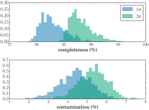
Figure 5 presents the $D_{kl}$ grid for all the different galaxy pairs for both $1\sigma$ and $2\sigma$ limits, labelling each galaxy by its index in our catalogue. We note that the asymmetry of the energy distributions and in the definition of the $D_{kl}$ carry through to an asymmetry in divergence space, and that $D_{kl}=0$ along the diagonal as there is no information lost in describing the energy distribution of galaxy $i$ as being drawn from the energy distribution of galaxy $i$. It is also clear that a larger degree of clustering is identified when the divergence limit is relaxed from $1\sigma$ to $2\sigma$, as this is a more generous criterion for associating energy distributions – this is consistent with our finding that the $2\sigma$ limit allows a higher level of completeness without significantly compromising the level of contamination. Where a set of objects emerges with mutually small divergences, these can be sorted into a ‘group’ or cluster; however, we note that the $D_{kl}$ strictly only sets upper limits on sets of groupable objects, as opposed to identifying groups. That is, given two objects with a $D_{kl}<2\sigma$, we can formally only say that these are compatible with being in the same group at the 2$\sigma$ level, given current observational limitations.

Figure 5: The Kullback-Leibler divergence $D_{kl}$ between all galaxy pairs. For identical distributions, $D_{kl}=0$, as can be seen down the diagonal. For an overlap between the two distributions $<1\sigma$ for a Gaussian distribution, $D_{kl}<0.5$. Hence coloured squares are indicative of pairs that may have been drawn from the same initial energy distribution. Left: with a $1\sigma$ cut-off in $D_{kl}$. Right: with a $2\sigma$ cut-off.

Figure 6: Left: Energy-position maps of the satellites, colour-coded according to the identified groups for the $2\sigma$ case. For each satellite, we use the energy and radius corresponding to the maximum of the probability distribution. Right: Probability distributions in energy for the satellites, colour-coded in the same groups. The clumps are much easier to pick out in this 1D space.

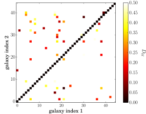
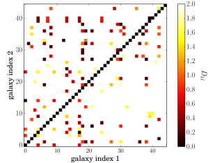
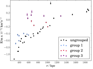
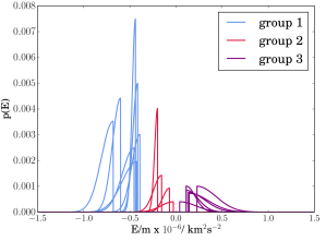
Table 2 summarises the groups that are identified in the $2\sigma$ case, and their distributions in both the 2D energy-position space and 1D energy space are shown in the middle and lower left-hand panels of Figure 6: for the former, we note that objects that are clustered in energy can be very dispersed in their positions on the sky, as might be expected to arise from phase mixing over the time since they started their infall, and that clustering can therefore be seen particularly clearly when plotted as a function of energy alone. With this $2\sigma$ limit, we find three clearly distinct clusters of galaxies with energies that appear to have been drawn from the same distribution, each with a small number of members (4, 6 and 7 objects); a remaining 28 objects do not appear to be associated with any others in this paradigm. We note that when we restrict our divergence limit to $1\sigma$, we find that the original groups fragment, and we end up with five clusters, each containing either two or three objects.

As a final test, we also examine the uncertainty introduced into our $D_{kl}$ analysis via uncertainties in $\alpha$, $\gamma$ and $\psi_{0}$. We do this by repeating the analysis for 100 samples of $(\alpha,\gamma,\psi_{0})$ drawn from their uncertainty distributions. We find the clustering to be robust against changes of the order of the uncertainties in all three parameters, but as long as correlations in the PDF between $\alpha$ and $\psi_{0}$ are accounted for correctly. That is, these two parameters are degenerate as they combine to describe the potential. Thus, drawing samples from the PDF assuming no covariance causes both parameters to be sampled too widely and thus begins to introduce uncertainty into the final object groupings. However, as long as the covariance is accounted for correctly, the same groupings are generally recovered at the $2\sigma$ level (with a small number of objects passing in and out of the larger groups across the samples). This is reassuring and suggests that our identification of substructure should not be significantly affected by our uncertainties on the potential and surface density.

ID	ra (deg)	dec (deg)	R (kpc)	$v_{\rm los}$ (kms-1)	$u$ (mag)	$g$ (mag)	$r$ (mag)	$i$ (mag)	$z$ (mag)
Group 1
1	186.92	13.08	309.76	-482.40	13.01	11.29	10.48	10.10	9.91
4	187.06	11.79	248.02	-609.60	15.48	13.66	12.89	12.39	12.40
5	187.24	13.24	287.81	-648.60	14.35	12.66	11.94	11.51	11.28
14	188.39	11.26	370.03	-521.40	16.61	15.56	14.85	14.49	14.25
18	188.55	12.05	257.81	750.20	16.29	14.92	14.21	13.81	13.60
8	187.47	14.07	504.22	269.80	13.85	12.15	11.39	11.00	10.76
25	189.23	12.52	453.82	363.85	15.91	14.25	13.63	13.33	13.05
Group 2
3	187.05	10.30	629.11	544.55	16.18	14.88	14.25	13.78	13.47
9	187.54	10.78	482.31	577.25	14.86	13.43	12.77	12.40	12.31
38	185.58	14.76	784.52	-299.05	16.59	15.42	14.71	14.34	14.01
43	186.42	12.81	402.81	-772.90	14.37	12.65	11.90	11.49	11.24
Group 3
7	187.45	13.43	318.31	1008.35	12.63	10.78	10.00	9.59	9.32
19	188.88	12.22	342.04	-902.70	13.78	12.17	11.42	11.03	10.77
20	188.91	12.38	352.58	-1023.75	16.82	15.11	14.34	13.94	13.65
22	188.92	12.56	363.50	-943.80	12.25	10.42	9.63	9.21	8.92
31	190.32	11.39	677.70	-708.75	15.92	14.17	13.40	13.01	12.78
39	186.02	11.22	505.59	800.20	14.77	13.15	12.44	12.04	11.81

Table 2: Galaxy clumps identified at the 2$\sigma$ level. Radii are clustocentric (taking M87 as the centre of the cluster) and line-of-sight velocities are also measured relative to M87; magnitudes are taken from SDSS DR7.

4 Discussion and Conclusions

Strong tests of the current cosmological paradigm are provided by the abundance of substructure. As larger structures are assembled hierarchically from mergers and accretion, we should be able to identify fossil signatures of these events in galaxies and clusters. In particular, galaxy clusters are characterised by a virialised region within which all components – galaxies and dark matter – are in dynamical equilibrium surrounded by infall zones in which groups of galaxies are falling into the relaxed cluster.

The identification of substructure has mainly been studied in the context of the Milky Way halo. Here, the existence of (in the best cases) six dimensional phase space coordinates makes the problem easier. For example, the use of the actions and frequencies (McMillan & Binney, 2008; Smith et al., 2009) has been advocated to identify past merger events in the Milky Way. The problem of the identification of substructure in projected datasets – in which only positions on the sky, line-of-sight velocities and heliocentric distances are available – is harder. It is also of much greater interest and applicability, both to nearby galaxies and to galaxy clusters.

Here, we have introduced a new formalism to describe the dynamical state of the outer parts of galaxies and galaxy clusters. The infalling motions of objects are assumed to be generated by purely radial orbits. This means that the probability distributions of observable quantities can be inferred, given the density of the infalling tracers and an estimate of the gravitational potential in which they move. We have provided a general algorithm to do this for spherical potentials. This enables us to search for infalling groups of objects, even though they may be scattered across the sky. Algorithms to quantify substructure in projected data are scarce. The only other one known to us looks for shells, which can be quantified by the characteristic “chevron pattern” discernible in line-of-sight velocity and position plots (Romanowsky et al., 2012).

As a practical application of our method, we have examined the dataset of satellite galaxies around M87. The extended envelope of M87 has been built from a deluge of smaller satellite galaxies, which may have accreted along preferred directions. Hence, we expect correlations in the satellite galaxy dataset, as some of the satellites may have fallen in along the same orbital path. Our algorithm exploits these correlations to identify kinematically similar substructure. In the case of M87, we have identified a number of possible galaxy associations. These are satellite galaxies whose position and kinematics are consistent with infall on the same radial path. This is expected in theories like $\Lambda$CDM in which the infall of satellites is coherent rather than random. This provides proof of principle that our algorithm can be applied to real data to extract useful results.

A possible test of the galaxy associations around M87 may be afforded by deep photometry of the candidates to find the position angles of the major axis. Infalling objects are expected to be stretched out along the orbital path, and so – if they lie on the orbits conjectured in this paper – they will be radially distended and their major axes will point towards M87. This effect is seen in the accretion of subhaloes in dissipationless simulations (Kuhlen et al., 2007; Barber et al., 2015) and persists with the inroduction of baryons (Knebe et al., 2010). Radial alignment has also been detected observationally in galaxy clusters and groups (see e.g., Hawley & Peebles, 1975; Agustsson & Brainerd, 2006), though the magnitude of this effect is unclear. However, we would predict significant isophotal alignment of the major axis of our candidates with the cluster radial direction if our associations are real.

Another natural application is to globular cluster and satellite galaxy datasets in other nearby galaxies. There are intense observational efforts focussing on completing the surveys of stellar streams and substructure around the Milky Way; however, a complete picture can only be obtained by studying a wider sample of galaxies at greater distances, although this is a much harder problem observationally. A good place to start would be with the satellites and clusters of M31, where coherent streams are readily visible; slightly further afield, the Centaurus group may also be a good candidate. We also note that M87 has a very large number of globular clusters (Oldham & Auger, 2016a) which may provide additional insights into the accretion history of the galaxy we have studied in this work. We anticipate that this algorithm will be a valuable tool in helping to investigate the build up of structure in the Local Group and beyond.

It is surprising that DFs built from only radial orbits have not received much more attention. Perhaps this is because for the fully self-consistent problem (in which the density generates the potential), such DFs fall foul of the radial orbit instability (Fridman & Polyachenko, 1984). However, this objection does not apply to tracer populations, which are moving in an external potential provided largely by other stellar and dark matter populations. We have shown that the radial orbit DF can always be found by Abel transforms via an inversion similar to Eddington (1916)’s classical work for the isotropic DF. In fact, radial orbit DFs are applicable to a wide range of astrophysical problems. In this paper, we have concentrated on material infalling onto BCGs, but the DFs are also applicable to populations expelled from central nuclei. The hypervelocity stars in the Milky Way are believed to be ejected by the central black hole with speeds from a few hundred to a few thousand kms^-1. The runaway stars are formed when one component of binary receives a kick as its companion explodes as a supernovae. Both hypervelocity and runaway stars are ejected from the central parts of the Milky Way with such high velocities that they move on almost radial orbits, as shown by simulations of their space motion by  Kenyon et al. (2014). Our DFs should have a ready application to the descriptions of these radially ejected populations as well.

Appendix A Numerical Constants

This appendix gives the three normalisation constants for power-law tracers in power-law potentials moving on radial orbits (see Section 2.2)

$$N_{0} = {\pi^{3/2}\Gamma([2\gamma+\alpha-4]/(2\alpha))\over\sqrt{2}r_{0}^{2}\Gamma([\gamma+\alpha-2]/\alpha)}F_{0}\psi_{0}^{(\gamma-2)/\alpha}$$

$$S_{0} = {\pi^{2}\Gamma([\gamma-1]/2)\Gamma([2\gamma+\alpha-4]/(2\alpha))\over\sqrt{2}r_{0}\Gamma(\gamma/2)\Gamma([\gamma+\alpha-2]/\alpha)}F_{0}\psi_{0}^{(\gamma-2)/\alpha}$$

$$v_{0}^{2} = {\psi_{0}\Gamma(\gamma/2)\Gamma([\alpha+\gamma-1)/2]\over 2\Gamma((\gamma-1)/2)\Gamma([\alpha+\gamma+2]/2)}.$$ (25)

References

- Agustsson & Brainerd (2006) Agustsson, I., & Brainerd, T. G. 2006, ApJL, 644, L25
- Barber et al. (2015) Barber, C., Starkenburg, E., Navarro, J. F., & McConnachie, A. W. 2015, MNRAS, 447, 1112
- Binggeli et al. (1985) Binggeli, B., Sandage, A., & Tammann, G. A. 1985, AJ, 90, 1681
- Binney & Tremaine (1987) Binney J., Tremaine S. 1987, Galactic Dynamics, Princeton University Press, Princeton
- Blakeslee et al. (2009) Blakeslee J. P., Jordán A., Mei S., Côté P., Ferrarese L., Infante L., Peng E. W., Tonry J. L., West M. J., 2009, ApJ, 694, 556
- Bowden et al. (2014) Bowden, A., Evans, N. W., & Belokurov, V. 2014, ApJL, 793, L42
- Bryan et al. (2012) Bryan, S. E., Mao, S., Kay, S. T., et al. 2012, MNRAS, 422, 1863
- Bullock & Johnston (2005) Bullock, J. S., & Johnston, K. V. 2005, ApJ, 635, 931
- Cooper et al. (2015) Cooper, A. P., Gao, L., Guo, Q., et al. 2015, MNRAS, 451, 2703
- Côté et al. (2003) Côté, P., McLaughlin, D. E., Cohen, J. G., & Blakeslee, J. P. 2003, ApJ, 591, 850
- Cuesta et al. (2008) Cuesta, A. J., Prada, F., Klypin, A., & Moles, M. 2008, MNRAS, 389, 385
- Eddington (1916) Eddington, A. S. 1916, MNRAS, 76, 572
- Falco et al. (2013) Falco, M., Mamon, G. A., Wojtak, R., Hansen, S. H., & Gottlöber, S. 2013, MNRAS, 436, 2639
- Fridman & Polyachenko (1984) Fridman, A., Polyachenko, V. 1984, Physics of Self-Gravitating Systems, Springer Verlag, New York
- Gonzalez et al. (2005) Gonzalez, A. H., Zabludoff, A. I., & Zaritsky, D. 2005, ApJ, 618, 195
- Hansen & Moore (2006) Hansen, S. H., & Moore, B. 2006, New Ast, 11, 333
- Hawley & Peebles (1975) Hawley, D. L., & Peebles, P. J. E. 1975, AJ, 80, 477
- Hopkins et al. (2010) Hopkins, P. F., Bundy, K., Hernquist, L., Wuyts, S., & Cox, T. J. 2010, MNRAS, 401, 1099
- Ibata et al. (2013) Ibata, R. A., Lewis, G. F., Conn, A. R., et al. 2013, Nat, 493, 62
- Kenyon et al. (2014) Kenyon, S. J., Bromley, B. C., Brown, W. R., & Geller, M. J. 2014, ApJ, 793, 122
- Kim et al. (2014) Kim S., Rey S.-C., Jerjen H., Lisker T., Sung E.-C., Lee Y., Chung J., Pak M., Yi W., Lee W., 2014, ApJSuppl. Ser., 215, 22
- Koposov et al. (2015) Koposov, S. E., Belokurov, V., Torrealba, G., & Evans, N. W. 2015, ApJ, 805, 130
- Kuhlen et al. (2007) Kuhlen, M., Diemand, J., & Madau, P. 2007, ApJ, 671, 1135
- Kullback & Leibler (1951) Kullback, S., Leibler, R. A. 1951, Ann. Math. Stat., 22, 79
- Knebe et al. (2010) Knebe, A., Libeskind, N. I., Knollmann, S. R., et al. 2010, MNRAS, 405, 1119
- Laporte et al. (2013) Laporte, C. F. P., White, S. D. M., Naab, T., & Gao, L. 2013, MNRAS, 435, 901
- Longobardi et al. (2015) Longobardi, A., Arnaboldi, M., Gerhard, O., & Mihos, J. C. 2015, AA, 579, L3
- Mackey et al. (2010) Mackey, A. D., Huxor, A. P., Ferguson, A. M. N., et al. 2010, ApJL, 717, L11
- McMillan & Binney (2008) McMillan, P. J., & Binney, J. J. 2008, MNRAS, 390, 429
- Mei et al. (2007) Mei, S., Blakeslee, J. P., Côté, P., et al. 2007, ApJ, 655, 144
- Naab et al. (2009) Naab, T., Johansson, P. H., & Ostriker, J. P. 2009, ApJL, 699, L178
- Oldham & Auger (2016a) Oldham, L. J., & Auger, M. W. 2016, MNRAS, 455, 820
- Oldham & Auger (2016b) Oldham, L. J., & Auger, M. W. 2016, MNRAS, 457, 421
- Prada et al. (2012) Prada, F., Klypin, A. A., Cuesta, A. J., Betancort-Rijo, J. E., & Primack, J. 2012, MNRAS, 423, 3018
- Romanowsky et al. (2012) Romanowsky, A. J., Strader, J., Brodie, J. P., et al. 2012, ApJ, 748, 29 Martínez-Delgado, D., Martin, N. F., et al. 2016, MNRAS, 457, L103
- Sanderson et al. (2015) Sanderson, R. E., Helmi, A., & Hogg, D. W. 2015, ApJ, 801, 98
- Sarli et al. (2014) Sarli, E., Meyer, S., Meneghetti, M., et al. 2014, AA, 570, A9
- Schuberth et al. (2010) Schuberth, Y., Richtler, T., Hilker, M., et al. 2010, AA, 513, A52
- Shen et al. (2003) Shen, S., Mo, H. J., White, S. D. M., et al. 2003, MNRAS, 343, 978
- Smith et al. (2009) Smith, M. C., Evans, N. W., Belokurov, V., et al. 2009, MNRAS, 399, 1223
- Tal et al. (2009) Tal, T., van Dokkum, P. G., Nelan, J., & Bezanson, R. 2009, AJ, 138, 1417
- Trujillo et al. (2007) Trujillo, I., Conselice, C. J., Bundy, K., et al. 2007, MNRAS, 382, 109
- van Dokkum et al. (2008) van Dokkum, P. G., Franx, M., Kriek, M., et al. 2008, ApJL, 677, L5
- Wojtak et al. (2008) Wojtak, R., Łokas, E. L., Mamon, G. A., et al. 2008, MNRAS, 388, 815
- Williams & Evans (2015) Williams, A. A., & Evans, N. W. 2015, MNRAS, 454, 698
- Xue et al. (2011) Xue, X.-X., Rix, H.-W., Yanny, B., et al. 2011, ApJ, 738, 79