A projection-based time-splitting algorithm for approximating nematic liquid crystal flows with stretching

Abstract.

A numerical method is developed for solving a system of partial differential equations modeling the flow of a nematic liquid crystal fluid with stretching effect, which takes into account the geometrical shape of its molecules. This system couples the velocity vector, the scalar pressure and the director vector representing the direction along which the molecules are oriented. The scheme is designed by using finite elements in space and a time-splitting algorithm to uncouple the calculation of the variables: the velocity and pressure are computed by using a projection-based algorithm and the director is computed jointly to an auxiliary variable. Moreover, the computation of this auxiliary variable can be avoided at the discrete level by using piecewise constant finite elements in its approximation. Finally, we use a pressure stabilization technique allowing a stable equal-order interpolation for the velocity and the pressure. Numerical experiments concerning annihilation of singularities are presented to show the stability and efficiency of the scheme.

Mathematics Subject Classification: Nematic liquid crystal; Finite elements; Projection method; Time-splitting method.

Keywords: 35Q35, 65M60, 76A15

1. Introduction

For a long time we have all believed that matter only existed in three states: solid, liquid, and gas. However, liquid crystals are substances that combine features of both isotropic liquids and crystalline solids, exhibiting intermediate transitions between solid and liquid phases, called mesophases. This behavior is due, in part, to the fact that liquid crystals are made up of macromolecules of similar size. Moreover it is well-known that the shape of the molecules plays an important role in the flow regimes of liquid crystal fluids. Thus, in general, different behaviors are expected for the dynamics of liquid crystal fluids being constituted by molecules of different shapes. For instance, liquid crystal fluids built from disk-shaped molecules may exhibit strikingly different properties from those composed of rod-shape materials.

The mathematical theory for the hydrodynamics of liquid crystal fluids was initiated by Ericksen [8, 9], and Leslie [15, 16]. Such a theory describes liquid crystals according to the different degrees of positional and orientational ordering of their molecules. The former refers to the relative position, on average, of the molecules or groups of molecules, while the latter alludes to the fact that the molecules tend to be locally aligned toward a specific and preferred direction, described by a unit vector, called director, defined according to the form of the molecules.

Within the liquid crystal phases, we find the so-called nematic phase. In it, the molecules have no positional order, but they self-organize to have long-range directional order. Thus, the molecules flow freely and their center of mass positions are randomly distributed as in a liquid, while maintain their long-range directional order. The breakdown of the self-alignment causes the appearance of defects or singularities which are able to significantly influence the flow behavior.

In this paper we are interested in the numerical solution of the flow of a nematic liquid crystal governed by an Ericksen-Leslie-type system which incorporates the stretching effect. This stretching effect comes from the kinematic transport of the director field, which depends on the shape of the molecules.

Let $T>0$ be a fixed time and let $\Omega\subset\mathbb{R}^{M},M=2$ or $3$, be a bounded open set with boundary $\partial\Omega$. Set $Q=\Omega\times(0,T]$ and $\Sigma=\partial\Omega\times(0,T]$. Then the equations are written as follows (see [17], [18] for more physical background, derivation, and discussion):

$$\left\{\begin{array}[]{rcl}\partial_{t}{\boldsymbol{d}}+({\boldsymbol{u}}\cdot\nabla){\boldsymbol{d}}+\beta(\nabla{\boldsymbol{u}}){\boldsymbol{d}}+(1+\beta)(\nabla{\boldsymbol{u}})^{T}{\boldsymbol{d}}+\gamma({\boldsymbol{f}}(\varepsilon,{\boldsymbol{d}})-\delta{\boldsymbol{d}})&=&\boldsymbol{0}\quad\mbox{ in $Q$,}\\ \partial_{t}{\boldsymbol{u}}+({\boldsymbol{u}}\cdot\nabla){\boldsymbol{u}}-\nu\delta{\boldsymbol{u}}+\nabla p+\lambda\nabla\cdot((\nabla{\boldsymbol{d}})^{T}\nabla{\boldsymbol{d}})&&\\ +\lambda\nabla\cdot(\beta({\boldsymbol{f}}(\varepsilon,{\boldsymbol{d}})-\delta{\boldsymbol{d}}){\boldsymbol{d}}^{T}+(1+\beta){\boldsymbol{d}}({\boldsymbol{f}}(\varepsilon,{\boldsymbol{d}})-\delta{\boldsymbol{d}})^{T})&=&\boldsymbol{0}\quad\mbox{ in $Q$,}\\ \nabla\cdot\,{\boldsymbol{u}}&=&0\quad\mbox{ in $Q$.}\end{array}\right.$$ (1)

We complete this system with homogeneous Dirichlet conditions for the velocity field (non-slip) and homogeneous Neumann boundary conditions for the director field:

$${\boldsymbol{u}}({\boldsymbol{x}},t)=\boldsymbol{0},\quad\partial_{{\boldsymbol{n}}}{\boldsymbol{d}}({\boldsymbol{x}},t)=\boldsymbol{0}\quad\mbox{ for $({\boldsymbol{x}},t)\in\Sigma$,}$$ (2)

and the initial conditions

$${\boldsymbol{d}}(\textit{{x}},0)={\boldsymbol{d}}_{0}(\textit{{x}}),\quad\quad{\boldsymbol{u}}(\textit{{x}},0)={\boldsymbol{u}}_{0}(\textit{{x}})\quad\mbox{ for ${\boldsymbol{x}}\in{\Omega}$.}$$ (3)

In system (1), ${\boldsymbol{u}}:\overline{Q}\to\mathbb{R}^{M}$ is the velocity of the liquid crystal flow, $p:\overline{Q}\to\mathbb{R}$ is the pressure, and ${\boldsymbol{d}}:\overline{Q}\to\mathbb{R}^{M}$ is the orientation of the molecules. The physical parameters $\nu$, $\lambda$ and $\gamma$ stand for positive constants which represent viscosity, elasticity, and relaxation time, respectively. The geometrical parameter $\beta\in[-1,0]$ is a constant associated with the aspect ratio of the ellipsoid particles. For instance, $\beta=-1/2,-1$ and $0$, corresponds to spherical, rod-like and disk-like liquid crystal molecules [14], respectively. Moreover, $\varepsilon>0$ is the penalty parameter and ${\boldsymbol{f}}(\varepsilon,{\boldsymbol{d}})$ is the penalty function related to the constraint $|{\boldsymbol{d}}|=1$. This penalty term can also be physically meaningful and represents a possible extensibility of molecules. It is defined by

$${\boldsymbol{f}}(\varepsilon,{\boldsymbol{d}})=\frac{1}{\varepsilon^{2}}\left(|{\boldsymbol{d}}|^{2}-1\right){\boldsymbol{d}}.$$ (4)

It should be noted that ${\boldsymbol{f}}(\varepsilon,{\boldsymbol{d}})=\nabla_{\boldsymbol{d}}F(\varepsilon,{\boldsymbol{d}})$, for all ${\boldsymbol{d}}\in{\rm I}\hskip-2.41849pt{\rm R}^{M}$, for the following scalar potential function

$$F(\varepsilon,{\boldsymbol{d}})=\frac{1}{4\varepsilon^{2}}(|{\boldsymbol{d}}|^{2}-1)^{2}.$$

The following energy law for system (1) holds under some regularity assumptions for ${\boldsymbol{u}}$ and ${\boldsymbol{d}}$ [17, 18]:

$$\frac{d}{dt}{\mathcal{E}}({\boldsymbol{u}},{\boldsymbol{d}})+\nu\int_{\Omega}|\nabla{\boldsymbol{u}}|^{2}+\lambda\gamma\int_{\Omega}|-\delta{\boldsymbol{d}}+{\boldsymbol{f}}(\varepsilon,{\boldsymbol{d}})|^{2}=0,$$ (5)

where

$${\mathcal{E}}({\boldsymbol{u}},{\boldsymbol{d}})=\frac{1}{2}\int_{\Omega}|{\boldsymbol{u}}|^{2}+\frac{\lambda}{2}\int_{\Omega}|\nabla{\boldsymbol{d}}|^{2}+\lambda\int_{\Omega}F(\varepsilon,{\boldsymbol{d}}).$$ (6)

The energy (6) expresses the competition between the kinetic and elastic energies. It should be noted that (5) is independent of $\varepsilon$ and $\beta$. Moreover, it provides a uniform bound for $F(\varepsilon,{\boldsymbol{d}})$ which leads to the unit sphere constraint in the limit as $\varepsilon\to 0$.

The mathematical structure of system (1) consists of the Navier-Stokes equations with some extra stress tensors taking into account the geometric of the molecules coupled with a gradient flow equation similar to that of harmonic maps into the sphere. The numerical resolution of system (1) is a nontrivial task due to the nonlinear nature of the system, the coupling terms between orientation and flow and the presence of the incompressibility constraint.

It is well known that time discretizations for the Navier–Stokes equations based on implicit time strategies give rise to highly time-consuming linear solver steps due to the coupled computation of both velocity and pressure. Furthermore, choices of stable finite element pairings are restricted by the inf–sup constraint. As a result, projection-based time-splitting techniques [11] turn to be a very favorable alternative to cutting down the computational cost of current iteration by successively updating velocity and pressure. It is obvious that such a strategy is desirable to solve system (1) in order to decouple the pressure computation from the velocity field as well as the computation of the director field. Instead, inf-sup conditions can be avoided by adding a pressure stabilizing term at the projection step, such that equal interpolation spaces for velocity and pressure are allowed. The stabilizing term is devised in such a way that the stability and convergence rate are not compromised [5].

There is an extensive literature on the mathematical analysis of finite element methods approximating system (1) without stretching effect, which corresponds to neglecting all the terms involving the paramter $\beta$. The interested reader is referred to the works [20, 19, 4, 10, 2, 3, 12, 6]. Very little has appeared for system (1) in the context of finite elements. In [17], Lin, Liu and Zhang presented a modified Crank-Nicolson scheme for which a discrete energy law is derived. As a solver, the author devised a fixed iterative method which gave rise to a matrix being symmetric and independent of time and the number of the fixed point iterations at each iteration. In [18], Liu, Lin and Zhang proposed a numerical algorithm based on a semi-implicit BDF2 rotational pressure-correction method for an axi-symmetric domain for studying the annihilation of a hedgehog-antihedgehog pair of defects. An extra term related to ${\boldsymbol{f}}(\varepsilon,{\boldsymbol{d}})$ was added so that the proposed scheme was somewhat unconditional, but no energy estimate was provided.

The goal of this paper is to use the above-mentioned techniques for the Navier-Stokes equations so as to be able to potentially enhance the performance of previous algorithms for system (1). In particular, we look for a numerical scheme using low-order finite-elements, which is linear at each time step and unconditionally stable and decouples the computation of the all primary variables. Moreover, we investigate the interplay of the flow of a nematic fluid and the geometric shape of its molecules in several numerical experiments.

The outline of the rest of this paper is the following. In section 2 we establish the function spaces, the notation and the hypotheses used in the work. Then the new numerical method are introduced. In section 3, we prove a priori estimates for the algorithm which provides the unconditional energy-stability property. The paper finishes with section 4, where some details about the implementation and numerical simulations that illustrate the performance of the scheme concerning the evolution of singularities are presented.

2. The numerical algorithm

2.1. Notation

For $1\leq p\leq\infty$, $L^{p}(\Omega)$ denotes the space of $p$th-power integrable real-valued functions defined on $\Omega$ for the Lebesgue measure. This space is a Banach space endowed with the norm $\|v\|_{L^{p}(\Omega)}=(\int_{\Omega}|v({\boldsymbol{x}})|^{p}\,{\rm d}{\boldsymbol{x}})^{1/p}$ for $1\leq p<\infty$ or $\|v\|_{L^{\infty}(\Omega)}={\rm ess}\sup_{{\boldsymbol{x}}\in\Omega}|v({\boldsymbol{x}})|$ for $p=\infty$. In particular, $L^{2}(\Omega)$ is a Hilbert space with the inner product

$$\left(u,v\right)=\int_{\Omega}u({\boldsymbol{x}})v({\boldsymbol{x}}){\rm d}{\boldsymbol{x}},$$

and its norm is simply denoted by $\|\cdot\|$. For $m$ a non-negative integer, we denote the classical Sobolev spaces as

$$H^{m}(\Omega)=\{v\in L^{2}(\Omega)\,;\,\partial^{k}v\in L^{2}(\Omega)\ \forall~{}|k|\leq m\},$$

associated to the norm

$$\|v\|_{H^{m}(\Omega)}=\left(\sum_{0\leq|k|\leq m}\|\partial^{k}v\|^{2}\right)^{1/2}\,,$$

where $k=(k_{1},\ldots,k_{M})\in{\mathds{N}^{M}}$ is a multi-index and $|k|=\sum_{i=1}^{M}k_{i}$, which is a Hilbert space with the obvious inner product. We will use boldfaced letters for spaces of vector functions and their elements, e.g. ${\boldsymbol{L}}^{2}(\Omega)$ in place of $L^{2}(\Omega)^{M}$.

Let $\mathcal{D}(\Omega)$ be the space of infinitely times differentiable functions with compact support on $\Omega$. The closure of ${\mathcal{D}}(\Omega)$ in $H^{m}(\Omega)$ is denoted by $H^{m}_{0}(\Omega)$. We will also make use of the following space of vector fields:

$${\boldsymbol{V}}=\{{\boldsymbol{v}v}\in\boldsymbol{\mathcal{D}}(\Omega):\nabla\cdot{\boldsymbol{v}v}=0\mbox{ in }\Omega\}.$$

We denote by ${\boldsymbol{H}}$ and ${\boldsymbol{V}}$, the closures of $\boldsymbol{\mathcal{V}}$, in the ${\boldsymbol{L}}^{2}(\Omega)$- and ${\boldsymbol{H}}^{1}(\Omega)$-norm, respectively, which are characterized (for $\Omega$ being Lipschitz-continuous) by (see [22])

$${\boldsymbol{H}} = \{{\boldsymbol{u}}\in{\boldsymbol{L}}^{2}(\Omega):\nabla\cdot{\boldsymbol{u}}=0\mbox{ in }\Omega,{\boldsymbol{u}}\cdot\boldsymbol{n}=0\hbox{ on }\partial\Omega\},$$

$${\boldsymbol{V}} = \{{\boldsymbol{u}}\in{\boldsymbol{H}}^{1}(\Omega):\nabla\cdot{\boldsymbol{u}}=0\mbox{ in }\Omega,{\boldsymbol{u}}=\boldsymbol{0}\hbox{ on }\partial\Omega\},$$

where ${\boldsymbol{n}}$ is the outward normal to $\Omega$ on $\partial\Omega$. Finally, we consider

$$L^{2}_{0}(\Omega)=\{p\in L^{2}(\Omega):\ \int_{\Omega}p({\boldsymbol{x}})\,d{\boldsymbol{x}}=0\}.$$

2.2. Hypotheses

Herein we introduce the hypotheses that will be required along this work.

1. Let $\Omega$ be a bounded domain of ${\rm I}\hskip-2.41849pt{\rm R}^{M}$ with a polygonal or polyhedral Lipschitz-continuous boundary.

2. Let $\{{\mathcal{T}}_{h}\}_{h>0}$ be a family of regular, quasi-uniform subdivisions of $\overline{{\Omega}}$ made up of triangles or quadrilaterals in two dimensions and tetrahedra or hexahedra in three dimensions, so that $\overline{\Omega}=\cup_{K\in{\mathcal{T}}_{h}}K$.

3. Assume three sequences of finite-dimensional spaces $\{{\boldsymbol{d}}_{h}\}_{h>0}$, $\{{\boldsymbol{V}}_{h}\}_{h>0}$ and $\{Q_{h}\}_{h>0}$ associated with $\{{\mathcal{T}}_{h}\}_{h>0}$ such that ${\boldsymbol{D}}_{h}\subset{\boldsymbol{H}}^{1}(\Omega)$, ${\boldsymbol{V}}_{h}\subset{\boldsymbol{H}}^{1}_{0}(\Omega)$ and $P_{h}\subset H^{1}(\Omega)\cap L^{2}_{0}(\Omega)$. Also, consider an extra finite-element space $\{{\boldsymbol{W}}_{h}\}_{h>0}$ with ${\boldsymbol{W}}_{h}\subset{\boldsymbol{L}}^{2}(\Omega)$.

4. Suppose that $({\boldsymbol{u}}_{0},{\boldsymbol{d}}_{0})\in{\boldsymbol{H}}\times{\boldsymbol{H}}^{1}(\Omega)$ with $|{\boldsymbol{d}}_{0}|\leq 1$ a.e. in $\Omega$.

In particular, hypothesis $\rm(H3)$ allows us to consider equal-order finite-element spaces for velocity and pressure. For instance, let $\mathcal{P}_{1}(K)$ be the set of linear polynomials on a triangle or tetrahedron $K$. Thus the space of continuous, piecewise polynomial functions associated to ${\mathcal{T}}_{h}$ is denoted as

$$X_{h}=\left\{v_{h}\in{C}^{0}(\overline{\Omega})\;:\;v_{h}|_{K}\in\mathcal{P}_{1}(K),\ \forall K\in\mathcal{T}_{h}\right\},$$

and the set of piecewise constant functions as

$$Y_{h}=\{w_{h}\in L^{\infty}(\Omega)\;:\;w_{h}|_{K}\in\mathbb{R},\ \forall K\in{\mathcal{T}}_{h}\}.$$

We choose the following continuous finite-element spaces

$${\boldsymbol{d}}_{h}={\boldsymbol{X}}_{h},\quad{\boldsymbol{V}}_{h}={\boldsymbol{X}}_{h}\cap{\boldsymbol{H}}^{1}_{0}(\Omega)\quad\hbox{and}\quad P_{h}=X_{h}\cap L^{2}_{0}(\Omega),$$

for approximating the director, the velocity and the pressure, respectively. Additionally, we select the extra discontinuous finite-element ${\boldsymbol{W}}_{h}={\boldsymbol{Y}}_{h}$ to be the space for an auxiliary variable related to the vector director.

Observe that our choice of the finite-element spaces for velocity and pressure does not satisfy the discrete inf-sup condition

$$\|p_{h}\|_{L^{2}_{0}({\Omega})}\leq\alpha\sup_{{\boldsymbol{v}v}_{h}\in{\boldsymbol{V}}_{h}\setminus\{0\}}\frac{\Big{(}q_{h},\nabla\cdot{\boldsymbol{v}v}_{h}\Big{)}}{\|{\boldsymbol{v}v}_{h}\|_{H^{1}({\Omega})}}\quad\forall\,p_{h}\in P_{h},$$ (7)

for $\alpha>0$ independent of $h$.

The following proposition is concerned with an interpolation operator $I_{h}$ associated with the space ${\boldsymbol{d}}_{h}$. In fact, we can think of $I_{h}$ as the Scott-Zhang interpolation operator, see [21].

Proposition 1.

Assuming hypotheses $\rm(H1)$-$\rm(H3)$, there exists $I_{h}:{\boldsymbol{H}}^{1}(\Omega)\to{\boldsymbol{d}}_{h}$ an interpolation operator satisfying

$$\|{\boldsymbol{d}}-I_{h}{\boldsymbol{d}}\|\leq C_{app}\,h\|\nabla{\boldsymbol{d}}\|\quad\forall\,{\boldsymbol{d}}\in{\boldsymbol{H}}^{1}(\Omega),$$ (8)

$$\|I_{h}{\boldsymbol{d}}\|_{{\boldsymbol{L}}^{\infty}(\Omega)}\leq C_{sta}\|{\boldsymbol{d}}\|_{{\boldsymbol{L}}^{\infty}(\Omega)}\quad\forall\,{\boldsymbol{d}}\in{\boldsymbol{L}}^{\infty}(\Omega),$$ (9)

$$\|I_{h}{\boldsymbol{d}}\|_{{\boldsymbol{H}}^{1}(\Omega)}\leq C_{sta}\|{\boldsymbol{d}}\|_{{\boldsymbol{H}}^{1}(\Omega)}\quad\forall\,{\boldsymbol{d}}\in{\boldsymbol{H}}^{1}(\Omega),$$ (10)

where $C_{app}>0$ and $C_{sta}>0$ are constants independent of $h$.

2.3. Description of the scheme

As explained in the introduction, we aim to construct a numerical solution to system (1) that, at each time step, one only needs to solve a sequence of decoupled elliptic equations for director, velocity and pressure. In particular, the linear systems associated to director and pressure are symmetric; therefore, scalable parallel solvers can be defined. Instead, the linear system associated to velocity is block diagonal, which means that each component of velocity can be computed in parallel. This makes our time-splitting be very appealing for high performance computing.

The starting point to design our time-splitting method is the non-incremental velocity-correction method for the Navier-Stokes equations. Moreover, it is also rather standard to take an essentially quadratic truncated potential $\widetilde{F}(\varepsilon,{\boldsymbol{d}})$ instead of the “quartic” potential $F(\varepsilon,{\boldsymbol{d}})$. To be more precise, one considers

$$\widetilde{F}(\varepsilon,{\boldsymbol{d}})=\frac{1}{\varepsilon^{2}}\begin{cases}\displaystyle\frac{1}{4}(|{\boldsymbol{d}}|^{2}-1)^{2},&\mbox{ if }|{\boldsymbol{d}}|\leq 1,\\ \displaystyle(|{\boldsymbol{d}}|-1)^{2},&\mbox{ if }|{\boldsymbol{d}}|>1,\end{cases}$$ (11)

for which

$$\widetilde{\boldsymbol{f}}(\varepsilon,{\boldsymbol{d}})=\nabla_{\boldsymbol{d}}\widetilde{F}(\varepsilon,{\boldsymbol{d}})=\frac{1}{\varepsilon^{2}}\begin{cases}\displaystyle(|{\boldsymbol{d}}|^{2}-1){\boldsymbol{d}},&\mbox{ if }|{\boldsymbol{d}}|\leq 1,\\ \displaystyle 2(|{\boldsymbol{d}}|-1)\frac{{\boldsymbol{d}}}{|{\boldsymbol{d}}|},&\mbox{ if }|{\boldsymbol{d}}|>1.\end{cases}$$

Let $N\in\mathds{N}$ and let $k=T/N$ denote the time-step size. To start up the sequence of approximation solutions, we consider

$${\boldsymbol{d}}_{0h}=\mathcal{I}_{h}{\boldsymbol{d}}_{0}$$ (12)

and $({\boldsymbol{u}}_{0h},p_{0h})\in{\boldsymbol{V}}_{h}\times P_{h}$ such that

$$({\boldsymbol{u}}_{0h},\bar{\boldsymbol{u}}_{h})+(\nabla p_{0h},\bar{\boldsymbol{u}}_{h}) =({\boldsymbol{u}}_{0},\bar{\boldsymbol{u}}_{h}),$$ (13a)

$$(\nabla\cdot{\boldsymbol{u}}_{0h},\bar{p}_{h})+j(p_{0h},\bar{p}_{h}) =0,$$ (13b)

for all $(\bar{\boldsymbol{u}}_{h},\bar{p}_{h})\in{\boldsymbol{V}}_{h}\times P_{h}$. It should be noted that $\|{\boldsymbol{u}}_{0h}\|\leq C\|{\boldsymbol{u}}_{0}\|$ holds.

Then the algorithm reads as follows. Let $({\boldsymbol{d}}^{n}_{h},{\boldsymbol{u}}^{n}_{h})\in{\boldsymbol{d}}_{h}\times{\boldsymbol{V}}_{h}$ be given. For the $n+1$ time step, do the following steps:

1. Find $({\boldsymbol{d}}^{n+1}_{h},{\boldsymbol{w}}^{n+1}_{h})\in{\boldsymbol{d}}_{h}\times{\boldsymbol{W}}_{h}$ satisfying

   $$\left\{\begin{array}[]{rcl}\displaystyle\left(\frac{{\boldsymbol{d}}^{n+1}_{h}-{\boldsymbol{d}}^{n}_{h}}{k},\bar{\boldsymbol{w}}_{h}\right)+({\boldsymbol{u}}^{\star}_{h},(\nabla{\boldsymbol{d}}^{n}_{h})^{T}\bar{\boldsymbol{w}}_{h})-\beta({\boldsymbol{u}}^{\star\star}_{h},\nabla\cdot(\bar{\boldsymbol{w}}_{h}({\boldsymbol{d}}^{n}_{h})^{T}))&&\\ -(1+\beta)({\boldsymbol{u}}^{\star\star\star}_{h},\nabla\cdot({\boldsymbol{d}}^{n}_{h}\bar{\boldsymbol{w}}^{T}_{h}))+\gamma({\boldsymbol{w}}^{n+1}_{h},\bar{\boldsymbol{w}}_{h})&=&0,\\ \displaystyle(\nabla{\boldsymbol{d}}^{n+1}_{h},\nabla\bar{\boldsymbol{d}}_{h})+(\widetilde{\boldsymbol{f}}_{\varepsilon}({\boldsymbol{d}}^{n}_{h})+\frac{H_{F}}{2\varepsilon^{2}}({\boldsymbol{d}}^{n+1}_{h}-{\boldsymbol{d}}^{n}_{h}),\bar{\boldsymbol{d}}_{h})-({\boldsymbol{w}}^{n+1}_{h},\bar{\boldsymbol{d}}_{h})=0,\end{array}\right.$$ (14)

   for all $(\bar{\boldsymbol{d}}_{h},\bar{\boldsymbol{w}}_{h})\in{\boldsymbol{D}}_{h}\times{\boldsymbol{W}}_{h}$, where (see (18) below)

   $$H_{F}:=(M3^{2}+(M^{2}-M)2^{2})^{1/2}$$

   and

   $${\boldsymbol{u}}^{\star}_{h} = {\boldsymbol{u}}^{n}_{h}+3\lambda\,k\,(\nabla{\boldsymbol{d}}_{h}^{n})^{T}{\boldsymbol{w}}^{n+1}_{h},$$

   $${\boldsymbol{u}}^{\star\star}_{h} = {\boldsymbol{u}}^{n}_{h}-3\lambda\beta k\,\nabla\cdot({\boldsymbol{w}}^{n+1}_{h}({\boldsymbol{d}}^{n}_{h})^{T}),$$

   $${\boldsymbol{u}}^{\star\star\star}_{h} = {\boldsymbol{u}}^{n}_{h}-3\lambda(1+\beta)k\,\nabla\cdot({\boldsymbol{d}}^{n}_{h}({\boldsymbol{w}}^{n+1}_{h})^{T}).$$

2. Find $p^{n+1}_{h}\in P_{h}$ satisfying

   $$k(\nabla p^{n+1}_{h},\nabla\bar{p}_{h})+j(p^{n+1}_{h},\bar{p}_{h})-(\widetilde{\boldsymbol{u}}^{n+1}_{h},\nabla\bar{p}_{h})=0,$$ (15)

   for all $\bar{p}_{h}\in P_{h}$, with

   $$\widetilde{\boldsymbol{u}}^{n+1}_{h} = \frac{{\boldsymbol{u}}^{\star}_{h}+{\boldsymbol{u}}^{\star\star}_{h}+{\boldsymbol{u}}^{\star\star\star}_{h}}{3}$$

   $$= {\boldsymbol{u}}^{n}_{h}+\lambda\,k\,\Big{(}(\nabla{\boldsymbol{d}}_{h}^{n})^{T}{\boldsymbol{w}}^{n+1}_{h}-\beta\nabla\cdot({\boldsymbol{w}}^{n+1}_{h}({\boldsymbol{d}}^{n}_{h})^{T})-(1+\beta)\nabla\cdot({\boldsymbol{d}}^{n}_{h}({\boldsymbol{w}}^{n+1}_{h})^{T})\Big{)}$$

   and

   $$j(p^{n+1}_{h},\bar{p}_{h})=S\frac{1}{\nu}(p^{n+1}_{h}-\pi_{0}(p^{n+1}_{h}),\bar{p}_{h}-\pi_{0}(\bar{p}_{h})),$$

   where $S>0$ is an algorithmic constant, and $\pi_{0}$ is the $L^{2}$-orthogonal projection operator onto $Y_{h}$.

3. Find ${\boldsymbol{u}}_{n}^{n+1}\in{\boldsymbol{V}}_{h}$ satisfying

   $$\begin{array}[]{l}\displaystyle\left(\frac{{\boldsymbol{u}}^{n+1}_{h}-{\boldsymbol{u}}^{n}_{h}}{k},\bar{\boldsymbol{u}}_{h}\right)+c({\boldsymbol{u}}^{n}_{h},{\boldsymbol{u}}^{n+1}_{h},\bar{\boldsymbol{u}}_{h})+\nu(\nabla{\boldsymbol{u}}^{n+1}_{h},\nabla\bar{\boldsymbol{u}}_{h})+(\nabla p_{h}^{n+1},\bar{\boldsymbol{u}}_{h})\\ +(-\lambda(\nabla{\boldsymbol{d}}^{n}_{h})^{T}{\boldsymbol{w}}^{n+1}_{h}+\lambda\beta\,\nabla\cdot({\boldsymbol{w}}^{n+1}_{h}({\boldsymbol{d}}^{n}_{h})^{T})+\lambda(1+\beta)\,\nabla\cdot({\boldsymbol{d}}^{n}_{h}({\boldsymbol{w}}^{n+1}_{h})^{T}),\bar{\boldsymbol{u}}_{h})=0,\end{array}$$ (16)

   for all $\bar{\boldsymbol{u}}_{h}\in{\boldsymbol{V}}_{h}.$

To enforce the skew-symmetry of the trilinear convective term in (16), we have defined

$$c({\boldsymbol{u}}_{h},{\boldsymbol{v}v}_{h},{\boldsymbol{w}}_{h})=(({\boldsymbol{u}}_{h}\cdot\nabla){\boldsymbol{v}v}_{h},{\boldsymbol{w}}_{h})+\frac{1}{2}(\nabla\cdot{\boldsymbol{u}}_{h},{\boldsymbol{v}v}_{h}\cdot{\boldsymbol{w}}_{h})$$

for all ${\boldsymbol{u}}_{h},{\boldsymbol{v}v}_{h},{\boldsymbol{w}}_{h}\in{\boldsymbol{V}}_{h}$. Thus, $c({\boldsymbol{u}}_{h},{\boldsymbol{v}v}_{h},{\boldsymbol{v}v}_{h})=0$ for all ${\boldsymbol{u}}_{h},{\boldsymbol{v}v}_{h}\in{\boldsymbol{V}}_{h}$.

Since scheme (14)-(16) is linear, it suffices to prove its uniqueness, which follows easily by comparing two solutions [6].

The main characteristic of scheme (14)-(16) is that the approximations $({\boldsymbol{d}}^{n+1}_{h},{\boldsymbol{w}}^{n+1}_{h})$, $p^{n+1}_{h}$ and ${\boldsymbol{v}v}^{n+1}_{h}$ are performed successively. The use of the auxiliary variable ${\boldsymbol{w}}^{n+1}_{h}$ is just to be able to derive a priori energy estimates, although the computation of ${\boldsymbol{w}}^{n+1}_{h}$ can be avoided as will be seen in section 4.

Concerning the stabilizing term $j(\cdot,\cdot)$, other choices are feasible if one wants to improve the spatial convergence rate:

$$j(p_{h},\bar{p}_{h})=S\frac{h^{2}}{\nu}(\nabla p_{h}-\pi(\nabla p_{h}),\nabla\bar{p}_{h}-\pi(\nabla\bar{p}_{h})),$$

where $\pi$ could be the ${\boldsymbol{L}}^{2}(\Omega)$-orthogonal protection operator onto ${\boldsymbol{Y}}_{h}$ [7] or the Scott-Zhang operator into ${\boldsymbol{Y}}_{h}$ [1]. The latter is more appealing since no auxiliary variable is required to compute it.

3. A priori energy estimates

Let us begin by noting that the $ij$-component of the Hessian matrix of the truncated potential $\widetilde{F}(\varepsilon,{\boldsymbol{d}})$ with respect to ${\boldsymbol{d}}$ is given by

$$H_{\boldsymbol{d}}\widetilde{F}(\varepsilon,{\boldsymbol{d}})_{ij}=\frac{1}{\varepsilon^{2}}\begin{cases}\displaystyle 2d_{i}d_{j}+(|{\boldsymbol{d}}|^{2}-1)\delta_{ij},&\mbox{ if }|{\boldsymbol{d}}|\leq 1,\\ \displaystyle 2\frac{d_{i}d_{j}}{|{\boldsymbol{d}}|^{3}}+2\frac{|{\boldsymbol{d}}|-1}{|{\boldsymbol{d}}|}\delta_{ij},&\mbox{ if }|{\boldsymbol{d}}|>1.\end{cases}$$

We thus have

$$\begin{array}[]{rl}\widetilde{F}(\varepsilon,{\boldsymbol{d}}^{n+1})-\widetilde{F}(\varepsilon,{\boldsymbol{d}}^{n})&=\nabla_{\boldsymbol{d}}\widetilde{F}(\varepsilon,{\boldsymbol{d}}^{n})\cdot({\boldsymbol{d}}^{n+1}-{\boldsymbol{d}}^{n})\\ &+\displaystyle\frac{1}{2}({\boldsymbol{d}}^{n+1}-{\boldsymbol{d}}^{n})^{T}H_{\boldsymbol{d}}\widetilde{F}(\varepsilon,{\boldsymbol{d}}^{n+\theta})({\boldsymbol{d}}^{n+1}-{\boldsymbol{d}}^{n}),\end{array}$$ (17)

where ${\boldsymbol{d}}^{n+\theta}=\theta{\boldsymbol{d}}^{n+1}+(1-\theta){\boldsymbol{d}}^{n}$ for some $\theta\in(0,1)$. Since $\widetilde{F}(\varepsilon,\cdot)$ is essentially quadratic, each component of the associated Hessian is uniformly bounded as

$$\|H_{\boldsymbol{d}}\widetilde{F}(\varepsilon,\cdot)_{ij}\|^{2}_{L^{\infty}({\rm I}\hskip-2.41849pt{\rm R}^{M})}\leq\frac{1}{\varepsilon^{2}}(2+\delta_{ij}).$$

Hence, the Frobenius norm is bounded as

$$\left(\sum_{i,j}^{M}\|H_{\boldsymbol{d}}\widetilde{F}(\varepsilon,\cdot)_{ij}\|^{2}_{L^{\infty}({\rm I}\hskip-2.41849pt{\rm R}^{M})}\right)^{1/2}\leq\frac{1}{\varepsilon^{2}}H_{F},\mbox{ where }H_{F}=(M3^{2}+(M^{2}-M)2^{2})^{1/2}.$$ (18)

In particular, using the consistence of the Frobenius norm gives

$$\frac{1}{2}({\boldsymbol{d}}^{n+1}-{\boldsymbol{d}}^{n})^{T}H_{\boldsymbol{d}}\widetilde{F}(\varepsilon,{\boldsymbol{d}}^{n+\theta})({\boldsymbol{d}}^{n+1}-{\boldsymbol{d}}^{n})\leq\frac{H_{F}}{2\varepsilon^{2}}|{\boldsymbol{d}}^{n+1}-{\boldsymbol{d}}^{n}|^{2}.$$ (19)

Consequently, by adding to $\widetilde{\boldsymbol{f}}(\varepsilon,{\boldsymbol{d}}^{n})$ a large enough first-order linear dissipation term, $\displaystyle\widetilde{\boldsymbol{f}}(\varepsilon,{\boldsymbol{d}}^{n})+\frac{H_{F}}{2\varepsilon^{2}}({\boldsymbol{d}}^{n+1}-{\boldsymbol{d}}^{n})$, we have, from (17) and (19),

$$\left(\widetilde{\boldsymbol{f}}(\varepsilon,{\boldsymbol{d}}^{n})+\frac{H_{F}}{2\varepsilon^{2}}({\boldsymbol{d}}^{n+1}-{\boldsymbol{d}}^{n})\right)\cdot({\boldsymbol{d}}^{n+1}-{\boldsymbol{d}}^{n})\geq\widetilde{F}(\varepsilon,{\boldsymbol{d}}^{n+1})-\widetilde{F}(\varepsilon,{\boldsymbol{d}}^{n}).$$ (20)

This inequality will play an essential role for the energy-stability of scheme (14). To prove this, we denote the discrete energy as

$${\mathcal{E}}({\boldsymbol{u}}_{h},{\boldsymbol{d}}_{h})=\frac{1}{2}\|{\boldsymbol{u}}_{h}\|^{2}+\frac{\lambda}{2}\|\nabla{\boldsymbol{d}}_{h}\|^{2}+\lambda\int_{\Omega}\widetilde{F}(\varepsilon,{\boldsymbol{d}}_{h}).$$

We are now in a position to prove the following result concerning a local-in-time discrete energy estimate.

Lemma 2.

Under hypotheses $(\rm H1)$–$(\rm H4)$, it follows that, for any $k>0$, $h>0$ and $\varepsilon>0$, the corresponding solution $({\boldsymbol{u}}^{n+1}_{h},p^{n+1}_{h},{\boldsymbol{d}}^{n+1}_{h},{\boldsymbol{w}}^{n+1}_{h})$ of scheme (14)-(16) satisfies the following inequality:

$$\begin{array}[]{rl}\displaystyle{\mathcal{E}}({\boldsymbol{u}}^{n+1}_{h},{\boldsymbol{d}}^{n+1}_{h})-{\mathcal{E}}({\boldsymbol{u}}^{n}_{h},{\boldsymbol{d}}^{n}_{h})+k\left(\nu\|\nabla{\boldsymbol{u}}_{h}^{n+1}\|^{2}+\lambda\gamma\|{\boldsymbol{w}}^{n+1}_{h}\|^{2}\right)+\frac{\lambda}{2}\|\nabla({\boldsymbol{d}}^{n+1}_{h}-{\boldsymbol{d}}^{n}_{h})\|^{2}&\\ \displaystyle+\frac{1}{2}\Big{(}\|{\boldsymbol{u}}_{h}^{n+1}-\widehat{\boldsymbol{u}}^{n+1}_{h}\|^{2}+\|\widehat{\boldsymbol{u}}_{h}^{n+1}-\widetilde{\boldsymbol{u}}^{n+1}_{h}\|^{2}\Big{)}+k\,j(p^{n+1}_{h},p^{n+1}_{h})&\\ \displaystyle+\frac{1}{2}\frac{\|\widetilde{\boldsymbol{u}}^{n+1}_{h}-{\boldsymbol{u}}^{\star}_{h}\|^{2}+\|\widetilde{\boldsymbol{u}}^{n+1}_{h}-{\boldsymbol{u}}^{\star\star}_{h}\|^{2}+\|\widetilde{\boldsymbol{u}}^{n+1}_{h}-{\boldsymbol{u}}^{\star\star\star}_{h}\|^{2}}{3}&\\ \displaystyle+\frac{1}{2}\frac{\|{\boldsymbol{u}}^{\star}_{h}-{\boldsymbol{u}}^{n}_{h}\|^{2}+\|{\boldsymbol{u}}^{\star\star}_{h}-{\boldsymbol{u}}^{n}_{h}\|^{2}+\|{\boldsymbol{u}}^{\star\star\star}_{h}-{\boldsymbol{u}}^{n}_{h}\|^{2}}{3}&\leq 0.\end{array}$$ (21)

Proof.

We take $\bar{\boldsymbol{w}}_{h}=\lambda\,k\,{\boldsymbol{w}}^{n+1}_{h}$ in $\eqref{scheme3eq1}_{a}$ and $\bar{\boldsymbol{d}}_{h}=\lambda({\boldsymbol{d}}^{n+1}_{h}-{\boldsymbol{d}}^{n}_{h})$ in $\eqref{scheme3eq1}_{b}$ and use (20) to obtain

$$\begin{array}[]{rl}\displaystyle\frac{\lambda}{2}\left(\|\nabla{\boldsymbol{d}}^{n+1}_{h}\|^{2}-\|\nabla{\boldsymbol{d}}^{n}_{h}\|^{2}+\widetilde{F}(\varepsilon,{\boldsymbol{d}}^{n+1}_{h})-\widetilde{F}(\varepsilon,{\boldsymbol{d}}^{n}_{h})\right)+\lambda\,\gamma\,k\|{\boldsymbol{w}}^{n+1}_{h}\|^{2}&\\ \displaystyle+\frac{\lambda}{2}\|\nabla({\boldsymbol{d}}^{n+1}_{h}-{\boldsymbol{d}}^{n}_{h})\|^{2}+\lambda\,k(({\boldsymbol{u}}^{\star}_{h},(\nabla{\boldsymbol{d}}^{n}_{h})^{T}{\boldsymbol{w}}^{n+1}_{h})\\ -\lambda\,k\,\beta\,({\boldsymbol{u}}^{\star\star}_{h},\nabla\cdot({\boldsymbol{w}}_{h}^{n+1}({\boldsymbol{d}}^{n}_{h})^{T}))-\lambda\,k\,(1+\beta)\,({\boldsymbol{u}}^{\star\star\star}_{h},\nabla\cdot({\boldsymbol{d}}^{n}_{h}({\boldsymbol{w}}^{n+1}_{h})^{T})&\leq 0.\end{array}$$ (22)

Next we take $\bar{\boldsymbol{u}}_{h}=k\,{\boldsymbol{u}}^{n+1}_{h}$, as a test function, in (16) and introduce the auxiliary velocity $\widehat{\boldsymbol{u}}^{n+1}_{h}=\widetilde{\boldsymbol{u}}^{n+1}_{h}-k\,\nabla p^{n+1}_{h}$ to obtain

$$\frac{1}{2}\|{\boldsymbol{u}}^{n+1}_{h}\|^{2}-\frac{1}{2}\|{\widehat{\boldsymbol{u}}}^{n+1}_{h}\|^{2}+\frac{1}{2}\|{\boldsymbol{u}}_{h}^{n+1}-{\widehat{\boldsymbol{u}}}^{n+1}_{h}\|^{2}+\nu\,k\|\nabla{\boldsymbol{u}}_{h}^{n+1}\|^{2}=0.$$ (23)

Now we take $\bar{p}_{h}=p^{n+1}_{h}$ in (15) and use the auxiliary velocity $\widehat{\boldsymbol{u}}^{n+1}_{h}$ introduced previously to obtain

$$\frac{1}{2}\|\widehat{\boldsymbol{u}}^{n+1}_{h}\|^{2}-\frac{1}{2}\|\widetilde{\boldsymbol{u}}^{n+1}_{h}\|^{2}+\frac{1}{2}\|\widehat{\boldsymbol{u}}^{n+1}_{h}-\widetilde{\boldsymbol{u}}^{n+1}_{h}\|^{2}+k\,j(p^{n+1}_{h},p^{n+1}_{h})=0.$$ (24)

From the definition of $\widetilde{\boldsymbol{u}}^{n+1}_{h}$ in (15), we write

$$\frac{\widetilde{\boldsymbol{u}}^{n+1}_{h}-{\boldsymbol{u}}^{\star}_{h}}{3}+\frac{\widetilde{\boldsymbol{u}}^{n+1}_{h}-{\boldsymbol{u}}^{\star\star}_{h}}{3}+\frac{\widetilde{\boldsymbol{u}}^{n+1}_{h}-{\boldsymbol{u}}^{\star\star\star}_{h}}{3}=0.$$

Hence,

$$\frac{1}{2}\|\widetilde{\boldsymbol{u}}^{n+1}_{h}\|^{2}-\frac{1}{2}\frac{\|{\boldsymbol{u}}^{\star}_{h}\|^{2}+\|{\boldsymbol{u}}^{\star\star}_{h}\|^{2}+\|{\boldsymbol{u}}^{\star\star\star}_{h}\|^{2}}{3}+\frac{1}{2}\frac{\|\widetilde{\boldsymbol{u}}^{n+1}_{h}-{\boldsymbol{u}}^{\star}_{h}\|^{2}+\|\widetilde{\boldsymbol{u}}^{n+1}_{h}-{\boldsymbol{u}}^{\star\star}_{h}\|^{2}+\|\widetilde{\boldsymbol{u}}^{n+1}_{h}-{\boldsymbol{u}}^{\star\star\star}_{h}\|^{2}}{3}=0.$$ (25)

Moreover, from the definitions of ${\boldsymbol{u}}^{\star}_{h}$, ${\boldsymbol{u}}^{\star\star}_{h}$ and ${\boldsymbol{u}}^{\star\star\star}_{h}$ in $\eqref{scheme3eq1}_{a}$, we deduce the following equalities:

$$\frac{1}{6}\|{\boldsymbol{u}}^{\star}_{h}\|^{2}-\frac{1}{6}\|{\boldsymbol{u}}^{n}_{h}\|^{2}+\frac{1}{6}\|{\boldsymbol{u}}^{\star}_{h}-{\boldsymbol{u}}^{n}_{h}\|^{2}-\lambda\,k\,((\nabla{\boldsymbol{d}}^{n}_{h})^{T}{\boldsymbol{w}}^{n+1}_{h},{\boldsymbol{u}}^{\star}_{h}) = 0,$$ (26)

$$\frac{1}{6}\|{\boldsymbol{u}}^{\star\star}_{h}\|^{2}-\frac{1}{6}\|{\boldsymbol{u}}^{n}_{h}\|^{2}+\frac{1}{6}\|{\boldsymbol{u}}^{\star\star}_{h}-{\boldsymbol{u}}^{n}_{h}\|^{2}+\lambda\,k\,\beta\,({\boldsymbol{u}}^{\star\star}_{h},\nabla\cdot({\boldsymbol{w}}_{h}^{n+1}({\boldsymbol{d}}^{n}_{h})^{T})) = 0,$$ (27)

$$\frac{1}{6}\|{\boldsymbol{u}}^{\star\star\star}_{h}\|^{2}-\frac{1}{6}\|{\boldsymbol{u}}^{n}_{h}\|^{2}+\frac{1}{6}\|{\boldsymbol{u}}^{\star\star\star}_{h}-{\boldsymbol{u}}^{n}_{h}\|^{2}+\lambda\,k\,(1+\beta)\,({\boldsymbol{u}}^{\star\star\star}_{h},\nabla\cdot({\boldsymbol{d}}^{n}_{h}({\boldsymbol{w}}^{n+1}_{h})^{T}) = 0,$$ (28)

Adding equalities (23)-(28) leads to

$$\begin{array}[]{rl}\displaystyle\frac{1}{2}\|{\boldsymbol{u}}^{n+1}_{h}\|^{2}-\frac{1}{2}\|{\boldsymbol{u}}^{n}_{h}\|^{2}+\nu\,k\|\nabla{\boldsymbol{u}}_{h}^{n+1}\|^{2}+\lambda\,k\,((\nabla{\boldsymbol{d}}^{n}_{h})^{T}{\boldsymbol{w}}^{n+1}_{h},{\boldsymbol{u}}^{\star}_{h})&\\ \displaystyle+\frac{1}{2}\left(\|{\boldsymbol{u}}_{h}^{n+1}-{\widehat{\boldsymbol{u}}}^{n+1}_{h}\|^{2}+\|\widehat{\boldsymbol{u}}^{n+1}_{h}-\widetilde{\boldsymbol{u}}^{n+1}_{h}\|^{2}\right)+k\,j(p^{n+1}_{h},p^{n+1}_{h})&\\ \displaystyle+\frac{1}{2}\frac{\|\widetilde{\boldsymbol{u}}^{n+1}_{h}-{\boldsymbol{u}}^{\star}_{h}\|^{2}+\|\widetilde{\boldsymbol{u}}^{n+1}_{h}-{\boldsymbol{u}}^{\star\star}_{h}\|^{2}+\|\widetilde{\boldsymbol{u}}^{n+1}_{h}-{\boldsymbol{u}}^{\star\star\star}_{h}\|^{2}}{3}&\\ \displaystyle+\frac{1}{2}\frac{\|{\boldsymbol{u}}^{\star}_{h}-{\boldsymbol{u}}^{n}_{h}\|^{2}+\|{\boldsymbol{u}}^{\star\star}_{h}-{\boldsymbol{u}}^{n}_{h}\|^{2}+\|{\boldsymbol{u}}^{\star\star\star}_{h}-{\boldsymbol{u}}^{n}_{h}\|^{2}}{3}&\\ \displaystyle-\lambda\,k\,((\nabla{\boldsymbol{d}}^{n}_{h})^{T}{\boldsymbol{w}}^{n+1}_{h},{\boldsymbol{u}}^{\star}_{h})+\lambda\,k\,\beta\,({\boldsymbol{u}}^{\star\star}_{h},\nabla\cdot({\boldsymbol{w}}_{h}^{n+1}({\boldsymbol{d}}^{n}_{h})^{T}))&\\ \displaystyle+\lambda\,k\,(1+\beta)\,({\boldsymbol{u}}^{\star\star\star}_{h},\nabla\cdot({\boldsymbol{d}}^{n}_{h}({\boldsymbol{w}}^{n+1}_{h})^{T})&=0.\end{array}$$ (29)

Finally, we add (22) and (29); thus the terms $((\nabla{\boldsymbol{d}}^{n}_{h})^{T}{\boldsymbol{w}}^{n+1}_{h},{\boldsymbol{u}}^{\star}_{h})$, $({\boldsymbol{u}}^{\star\star}_{h},\nabla\cdot({\boldsymbol{w}}_{h}^{n+1}({\boldsymbol{d}}^{n}_{h})^{T}))$ and $({\boldsymbol{u}}^{\star\star\star}_{h},\nabla\cdot({\boldsymbol{d}}^{n}_{h}({\boldsymbol{w}}^{n+1}_{h})^{T})$ cancel out, and hence (21) holds. This finishes the proof. ∎

Now, it is not difficult to extend the previous local-in-time discrete energy estimate to a global-in-time one.

Theorem 3.

Assume that $\rm(H0)$-$\rm(H4)$ are satisfied. The discrete solution $\{({\boldsymbol{u}}^{n}_{h},{\boldsymbol{d}}_{h}^{n},{\boldsymbol{w}}^{n}_{h})\}_{n=0}^{N}$ of scheme (14)-(16) satisfies

$$\max_{r\in\{0,\cdots,N-1\}}\left\{{\mathcal{E}}({\boldsymbol{u}}^{r+1}_{h},{\boldsymbol{d}}^{r+1}_{h})+k\sum_{n=0}^{r}\left(\nu\|\nabla{\boldsymbol{u}}_{h}^{n+1}\|^{2}+\lambda\gamma\|{\boldsymbol{w}}^{n+1}_{h}\|^{2}\right)\right\}\leq{\mathcal{E}}({\boldsymbol{u}}_{0h},{\boldsymbol{d}}_{0h}).$$ (30)

Proof.

The proof follows easily from Lemma 2 and by summing over $n$. ∎

It remains to prove that the initial energy ${\mathcal{E}}({\boldsymbol{u}}_{0h},{\boldsymbol{d}}_{0h})$ is bounded independent of $(h,k,\varepsilon)$.

Lemma 4.

Assume that hypotheses $\rm(H1)$-$\rm(H4)$ hold. If $(h,\varepsilon)$ are chosen satisfying

$$\frac{h}{\varepsilon}\leq K,$$ (31)

for some constant $K>0$, then

$${\mathcal{E}}({\boldsymbol{u}}_{0h},{\boldsymbol{d}}_{0h})\leq C_{0}$$ (32)

for the initial approximations $({\boldsymbol{u}}_{0h},{\boldsymbol{d}}_{0h})$ defined in (12) and (13).

Proof.

We take $\bar{\boldsymbol{u}}={\boldsymbol{u}}_{0h}$ and $\bar{p}_{h}=p_{0h}$ as test functions into (13) to obtain

$$\frac{1}{2}\|{\boldsymbol{u}}_{0h}\|^{2}+j(p_{0h},p_{0h})\leq\frac{1}{2}\|{\boldsymbol{u}}_{0}\|^{2}.$$ (33)

Moreover, from (10), we have

$$\|{\boldsymbol{d}}_{0h}\|_{{\boldsymbol{H}}^{1}(\Omega)}\leq C\|{\boldsymbol{d}}_{0}\|_{{\boldsymbol{H}}^{1}(\Omega)}.$$ (34)

Now, we bound as in [12],

$$\displaystyle\int_{\Omega}F(\varepsilon,{\boldsymbol{d}}_{0h}) \leq \displaystyle\frac{1}{\varepsilon^{2}}\int_{\Omega}(|{\boldsymbol{d}}_{0h}|^{2}-|{\boldsymbol{d}}_{0}|^{2})^{2}=\frac{1}{\varepsilon^{2}}\int_{\Omega}(|{\boldsymbol{d}}_{0h}+{\boldsymbol{d}}_{0}||{\boldsymbol{d}}_{0h}-{\boldsymbol{d}}_{0}|)^{2}$$ (35)

$$\leq \displaystyle\|{\boldsymbol{d}}_{0h}+{\boldsymbol{d}}_{0}\|^{2}_{{\boldsymbol{L}}^{\infty}(\Omega)}\|{\boldsymbol{d}}_{0h}-{\boldsymbol{d}}_{0}\|^{2}\leq C\,\frac{h^{2}}{\varepsilon^{2}}\|{\boldsymbol{d}}_{0}\|^{2}_{{\boldsymbol{H}}^{1}(\Omega)},$$

where (8) and (9) has been applied. Combining (35) with (33) and (34) together with (31), we obtain (32). ∎

Remark 5.

Hypothesis (31) is rarely explicitly mentioned in numerical papers based on algorithms using the penalty approach but it is required to guarantee a priori energy estimates independent of $\varepsilon$. It seems that this condition is overlooked. Nevertheless, it is important to underline that the constraint (31) for $(h,\varepsilon)$ comes only from the approximation of ${\boldsymbol{d}}_{0}$ in ${\boldsymbol{D}}_{h}$ but not from the discrete scheme itself.

4. Numerical results

From now on, we consider the particular instance of the approximating spaces ${\boldsymbol{D}}_{h},{\boldsymbol{V}}_{h}$ and $P_{h}$ described in $\rm(H3)$. The main objective of this section is to illustrate the stability, efficiency and reliability of scheme (14)-(16). In doing so, we will present some numerical experiments concerning the annihilation of singularities, and use the results to check numerically how the stabilization constant $H_{F}$ must be chosen to assure the unconditional stability. The numerical solutions are calculated with a computer program implemented in FreeFem++ [13].

Before going further, we discuss some implementation issues concerning scheme (14)-(16).

4.1. Implementation issues

Let $N_{d}=\dim({\boldsymbol{D}}_{h})$, $N_{w}=\dim({\boldsymbol{W}}_{h})$ and let $\{{\boldsymbol{\phi}}^{d}_{i}\}_{i=1}^{N_{d}}$ and $\{{\boldsymbol{\phi}}^{w}_{i}\}_{i=1}^{N_{w}}$ be the finite-element bases for ${\boldsymbol{D}}_{h}$ and ${\boldsymbol{W}}_{h}$, respectively, constructed from the local basis of $X_{h}$ and $Y_{h}$, respectively. We describe the following matrices related to ${\boldsymbol{W}}_{h}$:

$${\boldsymbol{\mathsf{M}}}_{w,d}=\left(\int_{\Omega}{\boldsymbol{\phi}}_{i}^{d}\cdot{\boldsymbol{\phi}}_{j}^{w}\right)_{ij},\quad{\boldsymbol{\mathsf{M}}}_{w}=\left(\int_{\Omega}{\boldsymbol{\phi}}_{i}^{w}\cdot{\boldsymbol{\phi}}_{j}^{w}\right)_{ij},\quad\displaystyle{\boldsymbol{\mathsf{B}}}_{w}={\boldsymbol{\mathsf{B}}}^{\star}_{w}+{\boldsymbol{\mathsf{B}}}^{\star\star}_{w}+{\boldsymbol{\mathsf{B}}}^{\star\star\star}_{w},$$

where

$$\displaystyle{\boldsymbol{\mathsf{B}}}^{\star}_{w}=3\lambda k\left(\int_{\Omega}[\nabla{\boldsymbol{d}}_{h}^{n}]^{T}{\boldsymbol{\phi}}_{i}^{w}\cdot[\nabla{\boldsymbol{d}}^{n}_{h}]^{T}{\boldsymbol{\phi}}_{j}^{w}\right)_{ij},\quad{\boldsymbol{\mathsf{B}}}^{\star\star}_{w}=3\lambda\beta^{2}k\left(\int_{\Omega}\left[\nabla\cdot({\boldsymbol{\phi}}_{i}^{w}[{\boldsymbol{d}}_{h}^{n}]^{T})\right]\cdot\left[\nabla\cdot({\boldsymbol{\phi}}_{j}^{w}[{\boldsymbol{d}}^{n}_{h}]^{T})\right]\right)_{ij},$$

$$\displaystyle{\boldsymbol{\mathsf{B}}}^{\star\star\star}_{w}=3\lambda(1+\beta)^{2}k\left(\int_{\Omega}\left[\nabla\cdot({\boldsymbol{d}}_{h}^{n}[{\boldsymbol{\phi}}_{i}^{w}]^{T})\right]\cdot\left[\nabla\cdot({\boldsymbol{d}}^{n}_{h}[{\boldsymbol{\phi}}_{j}^{w}]^{T})\right]\right)_{ij}.$$

Also, we introduce the matrices related to ${\boldsymbol{D}}_{h}$:

$${\boldsymbol{\mathsf{M}}}_{d}=\left(\int_{\Omega}{\boldsymbol{\phi}}_{i}^{d}\cdot{\boldsymbol{\phi}}_{j}^{d}\right)_{ij},\quad{\boldsymbol{\mathsf{M}}}_{d,w}=\left(\int_{\Omega}{\boldsymbol{\phi}}_{i}^{w}\cdot{\boldsymbol{\phi}}_{j}^{d}\right)_{ij},\quad{\boldsymbol{\mathsf{L}}}_{d}=\left(\int_{\Omega}\nabla{\boldsymbol{\phi}}_{i}^{d}\cdot\nabla{\boldsymbol{\phi}}_{j}^{d}\right)_{ij}.$$

Moreover, let us denote by $\mathsf{W}\in\mathbb{R}^{N_{w}}$ and $\mathsf{D}\in\mathbb{R}^{N_{d}}$ the coordinate vectors, with respect to the fixed bases of the finite-element functions ${\boldsymbol{w}}_{h}\in{\boldsymbol{W}}_{h}$ and ${\boldsymbol{d}}_{h}\in{\boldsymbol{D}}_{h}$, respectively. Thus, we can rewrite system (14) as

$$\displaystyle\frac{1}{k}{\boldsymbol{\mathsf{M}}}_{w,d}\mathsf{D}^{n+1}+\left({\boldsymbol{\mathsf{B}}}_{w}+\gamma{\boldsymbol{\mathsf{M}}}_{w}\right)\mathsf{W}^{n+1} =\frac{1}{k}{\boldsymbol{\mathsf{M}}}_{w,d}\mathsf{D}^{n}-\mathsf{F}_{w},$$ (36a)

$${\boldsymbol{\mathsf{L}}}_{d}\mathsf{D}^{n+1}+\frac{H_{F}}{2\varepsilon^{2}}{\boldsymbol{\mathsf{M}}}_{d}\mathsf{D}^{n+1}-{\boldsymbol{\mathsf{M}}}_{d,w}\mathsf{W}^{n+1} =\mathsf{F},$$ (36b)

where $\displaystyle\mathsf{F}_{w}\in{\rm I}\hskip-2.41849pt{\rm R}^{N_{d}}$ and $\mathsf{F}\in{\rm I}\hskip-2.41849pt{\rm R}^{N_{w}}$ are defined, respectively, as

$$\displaystyle\mathsf{F}_{w}=\left(\int_{\Omega}{\boldsymbol{u}}_{h}^{n}\cdot\left[[\nabla{\boldsymbol{d}}^{n}_{h}]^{T}{\boldsymbol{\phi}}_{j}^{w}\right]-\beta\int_{\Omega}{\boldsymbol{u}}_{h}^{n}\cdot\left[\nabla\cdot({\boldsymbol{\phi}}_{j}^{w}({\boldsymbol{d}}^{n}_{h})^{T})\right]-(1+\beta)\int_{\Omega}{\boldsymbol{u}}_{h}^{n}\cdot\left[\nabla\cdot({\boldsymbol{d}}^{n}_{h}({\boldsymbol{\phi}}_{j}^{w})^{T}\right]\right)_{j},$$

$$\displaystyle\mbox{and }\mathsf{F}=\left(\int_{\Omega}\left[\frac{H_{F}}{2\varepsilon^{2}}{\boldsymbol{d}}^{n}_{h}-\tilde{\boldsymbol{f}}_{\varepsilon}({\boldsymbol{d}}^{n}_{h})\right]\cdot\phi_{j}^{d}\right)_{j}.$$

By defining ${\boldsymbol{\mathsf{E}}}_{w}={\boldsymbol{\mathsf{B}}}_{w}+\gamma{\boldsymbol{\mathsf{M}}}_{w}$, from (36a), we have

$$\mathsf{W}^{n+1}={\boldsymbol{\mathsf{E}}}^{-1}_{w}\left[\frac{1}{k}{\boldsymbol{\mathsf{M}}}_{w,d}\left(\mathsf{D}^{n}-\mathsf{D}^{n+1}\right)-\mathsf{F}_{w}\right],$$

where ${\boldsymbol{\mathsf{E}}}_{w}$ can be seen in two different ways depending on the reordering of the degrees of freedom of $\mathsf{W}^{n+1}$: (1) A block-diagonal, $M$-by-$M$ matrix, which is easy to invert by using a block Gauss-Jordan elimination method, or (2) an $M$-by-$M$ block, diagonal matrix, since the degrees of freedom of two different elements are not coupled, which is also easily invertible by using block computations. The first approach is much more adequate especially for legacy code bases, which is our case here.

Replacing the above equality in equations (36b), and after some calculations, the resulting system is:

$$\left({\boldsymbol{\mathsf{L}}}_{d}+\frac{1}{k}{\boldsymbol{\mathsf{M}}}_{d,w}{\boldsymbol{\mathsf{E}}}_{w}^{-1}{\boldsymbol{\mathsf{M}}}_{w,d}+\frac{H_{F}}{2\varepsilon^{2}}{\boldsymbol{\mathsf{M}}}_{d}\right)\mathsf{D}^{n+1}={\boldsymbol{\mathsf{M}}}_{d,w}{\boldsymbol{\mathsf{E}}}_{w}^{-1}\left[\frac{1}{k}{\boldsymbol{\mathsf{M}}}_{w,d}\mathsf{D}^{n}-\mathsf{F}_{w}\right]+\mathsf{F}.$$ (37)

Consequently, we can avoid, at algebraic level, computing the auxiliary vector $\mathsf{W}^{n+1}$ by solving directly $\eqref{linear-system}$. Observe that the matrix $\displaystyle{\boldsymbol{\mathsf{L}}}_{d}+\frac{1}{k}{\boldsymbol{\mathsf{M}}}_{d,w}{\boldsymbol{\mathsf{E}}}_{w}^{-1}{\boldsymbol{\mathsf{M}}}_{w,d}+\frac{H_{F}}{2\varepsilon^{2}}{\boldsymbol{\mathsf{M}}}_{d}$ is the Schur complement of system (36) with respect to ${\boldsymbol{\mathsf{E}}}_{w}$. Moreover, such a matrix is symmetric and positive definite.

4.2. Annihilation of singularities

In this experiment, we consider $\Omega=(-1,1)\times(-1,1)$ and the physical parameters $\nu=\lambda=\gamma=1$. Also, we take $\beta=-1$, that is, rod-like molecules of the liquid crystal are considered. The discretization, penalization and stabilization parameters are set as

$$k=0.001,h=0.0790796,\varepsilon=0.05,\mbox{ and }H_{F}=0.$$

Given an initial velocity ${\boldsymbol{v}v}_{0}$, the main objective of the experiment is to study the evolution of the singularities of the initial director ${\boldsymbol{d}}_{0}$, that is, points of the computational domain $\Omega$ where $|{\boldsymbol{d}}_{0}|=0$. In particular, we will present two numerical experiences concerning the annihilation of two and four singularities, respectively. Furthermore, we will show the behavior of the energies, the singularities and the velocity fields for each of these simulations. Let us begin with the case of two singularities.

4.2.1. Two singularities

This experiment was originally proposed for a nematic liquid crystal without stretching in [20] and, later extended for system (1) in [17]. In these works, Dirichlet boundary conditions for the director field were considered. In our case, we consider Neumann boundary conditions as in the results presented in [4] and [6]. The initial conditions of the problem are

$${\boldsymbol{u}}_{0}=\boldsymbol{0},\quad{\boldsymbol{d}}_{0}=\frac{\tilde{\boldsymbol{d}}}{\sqrt{|\tilde{\boldsymbol{d}}|^{2}+\varepsilon^{2}}},\mbox{ where }\tilde{\boldsymbol{d}}=(x^{2}+y^{2}-0.25,y).$$

In Figure 1, we present snapshots of the director and velocity fields displayed at times $t=0.0,0.1,0.2,0.3$. Initially, the two singularities are transported to the origin by the velocity field, which, at the beginning of the experiment, forms four vortices being transformed only into two at the end. The numerical results show that the behavior of the director field is analogous qualitatively to the corresponding director field for the model without stretching reported in [4] and [6]. On the other hand, quantitatively, we observe that the size of the time interval, where the dynamics takes place, is very different. In our case, the size of this interval is about three times smaller than in the case without stretching, causing the annihilation time to be smaller than that in [6]. Concerning the behavior of the velocity field, we find that both the magnitude and the dynamics of the velocity are quite different. The maximum values of the kinetic energy in [6] and now differ about two times each other, being bigger now with stretching. We start the computation with the formation of four vortices, and end up with two symmetrical vortices with respect to $y=0$, whilst, in [4] and [6], the four symmetrical vortices with respect to the origin keep so till the dynamics vanishes.

In Figure 2, we present the evolution of kinetic, elastic, and penalization energies, as well as the total energy. As predicted by inequality (21), the total energy decreases with time. Also, the kinetic energy reaches its maximum level at the annihilation time that in this case is at $t\thickapprox 0.242$. After this time, the system evolves to a steady state solution and all the energies decay quickly. Qualitatively, the graphics of the energies are similar to those reported in [4] and [6] for the model without stretching.

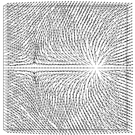
(a) $\|{\boldsymbol{d}}\|_{\infty}=0.9977852.$

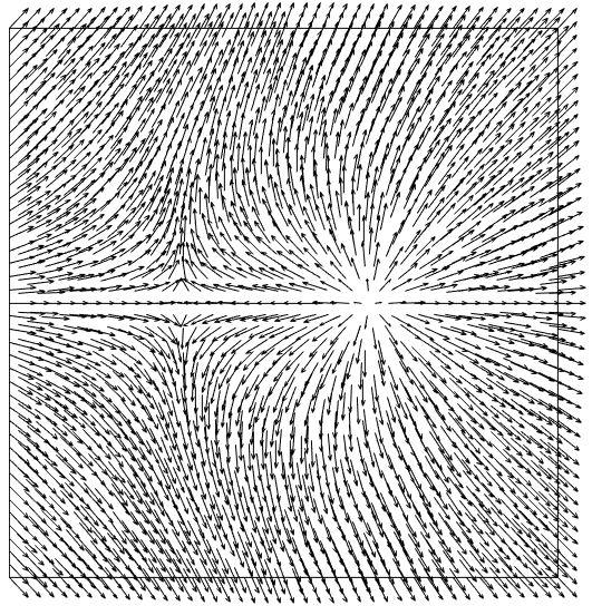
(b) $\|{\boldsymbol{d}}\|_{\infty}=0.9971739.$

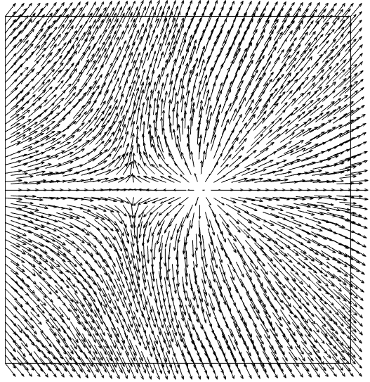
(c) $\|{\boldsymbol{d}}\|_{\infty}=0.9973484.$

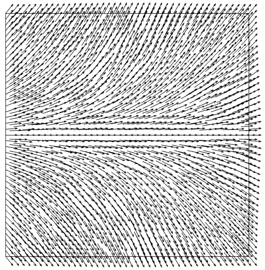
(d) $\|{\boldsymbol{d}}\|_{\infty}=0.9974461.$

(e) $\|{\boldsymbol{u}}\|_{\infty}=0.0.$

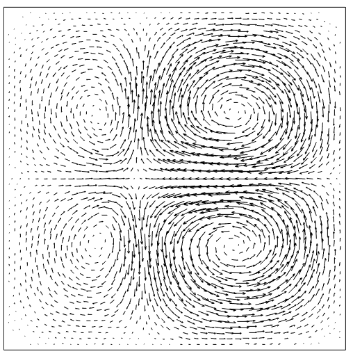
(f) $\|{\boldsymbol{u}}\|_{\infty}=0.289702.$

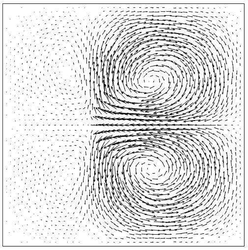
(g) $\|{\boldsymbol{u}}\|_{\infty}=0.4079601.$

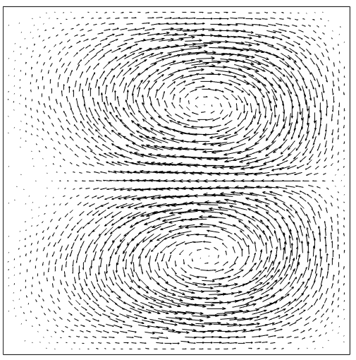
(h) $\|{\boldsymbol{u}}\|_{\infty}=0.2954702.$

Figure 1. Evolution of the director field (a)-(d) and the velocity field (e)-(h) for the annihilation of two singularities at times $t=0.0,0.1,0.2,0.3$. Here $\beta=-1$ and $H_{F}=0$.

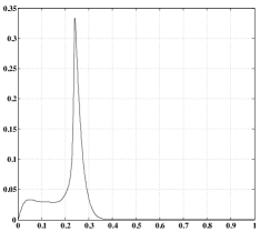
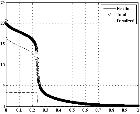
Figure 2. Evolution in time of the energies for the experiment of two singularities. Kinetic energy (left) and total, elastic, and penalization energies (right). Here $\beta=-1$ and $M=0$.

4.2.2. Four singularities

In this case, the initial director field has two singularities on the $x-$axis located at the points $(\pm 0.5,0)$ and two more singularities on the $y-$axis, located at the points $(0,\pm 0.25)$. More precisely, we consider the initial conditions

$${\boldsymbol{u}}_{0}=\boldsymbol{0},\quad{\boldsymbol{d}}_{0}=\frac{\tilde{\boldsymbol{d}}}{\sqrt{|\tilde{\boldsymbol{d}}|^{2}+\varepsilon^{2}}},\mbox{ where }\tilde{\boldsymbol{d}}=\left(\frac{x^{2}}{0.5^{2}}+\frac{y^{2}}{0.25^{2}}-1,-xy\right).$$

In Figure 3, we present snapshots of the director and velocity fields displayed at times $t=0.02,0.06,0.08$ and $0.12$. We observe that the dynamics of the four singularities is faster than in the two-singularity case. The two singularities located on the $x-$axis begin to move toward each other, while those located on the $y-$axis remains without moving till all the singularities are positioned at the same distance from the origin. Then they move uniformly to the origin and simultaneously disappear at the origin. This behavior is due to the dynamics of the velocity field in the $y-$axis, preventing the singularities located there from moving to the origin.

As in the case of two singularities, we note that the annihilation time is smaller than in[6]. Now, this time is at $t\thickapprox 0.071$ which is the half of the time reported in [6]. This behavior is due to the increase of the magnitude of the velocity field. Additionally, at the beginning of the experiment, we note the formation of four big vortices in each quadrant of the $xy$ plane and other four more close to the $y-$axis. This last four vortices disappear as time moves on. When the singularities annihilate, we note only three vortices in the velocity field.

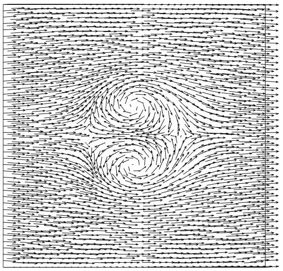
(a) $\|{\boldsymbol{d}}\|_{\infty}=0.9999915.$

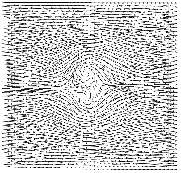
(b) $\|{\boldsymbol{d}}\|_{\infty}=0.9999619$

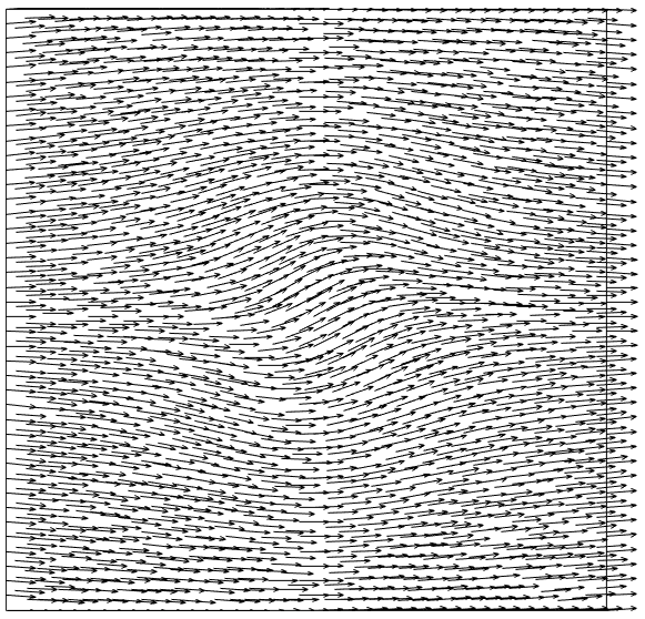
(c) $\|{\boldsymbol{d}}\|_{\infty}=0.9999404.$

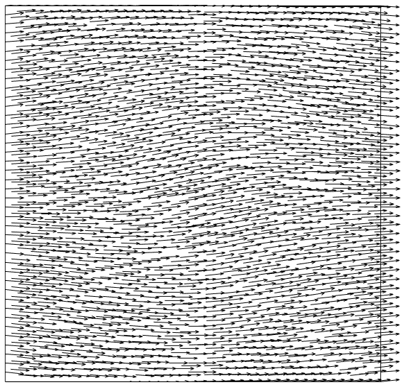
(d) $\|{\boldsymbol{d}}\|_{\infty}=0.9999247.$

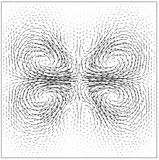
(e) $\|{\boldsymbol{u}}\|_{\infty}=1.21298.$

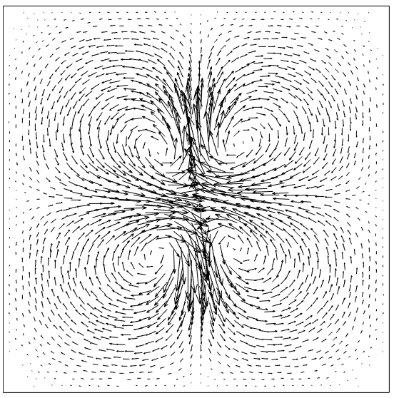
(f) $\|{\boldsymbol{u}}\|_{\infty}=1.765187.$

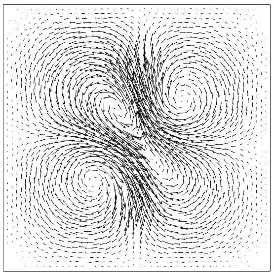
(g) $\|{\boldsymbol{u}}\|_{\infty}=1.299686.$

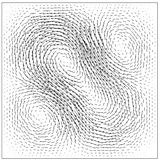
(h) $\|{\boldsymbol{u}}\|_{\infty}=0.2250148.$

Figure 3. Evolution of the director field (a)-(d) and the velocity field (e)-(h) for the annihilation of four singularities at times $t=0.02,0.06,0.08,0.12$. Here $\beta=-1$ and $H_{F}=0$.

The graphs of the energies are shown in Figure 4. In particular, we highlight that the maximum value of the kinetic energy is attained at about the annihilation time. On the other hand, as described in [6], such a maximum is reached at the very beginning of the simulation far away from the annihilation. The evolution of the other energies behaves similarly. The total and elastic energies decrease with time, whilst the penalized one presents an increase at the beginning to adopt a constant behavior and, finally, decreases with time after the annihilation of the singularities.

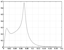
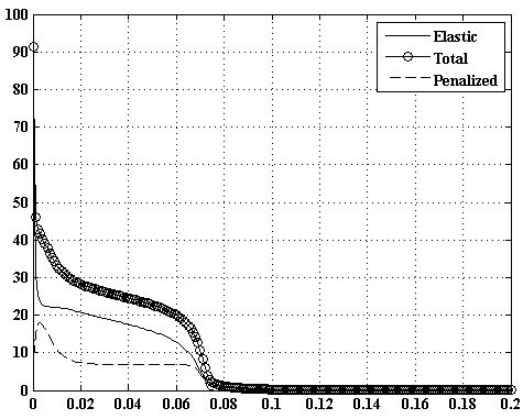
Figure 4. Evolution in time of the energies for the experiment of four singularities. Kinetic energy (left) and total, elastic, and penalization energies (right).

4.3. Stability dependence on $H_{F}$

Next, we carry out a sensitivity study of scheme (14)-(16). More precisely, we give a detailed look to the relation among the stabilization constant $H_{F}$ defined in (18), the geometrical parameter $\beta$ and the penalization parameter $\varepsilon$. The results were generated by considering the problems of annihilation of singularities described previously; see Tables 1, 4, 2 and 3.

Table 1. Stability dependence of scheme (14)-(16) on the parameters $M$ and $\beta$ for the annihilation of two singularities. In this case $\varepsilon=0.05,k=0.001$ and $h=0.0913931$. $T_{\max}$ is the time where the kinetic energy reaches its maximum value.

$\beta\backslash M$	0	0.5	1	1.5	2
	✓	✓	✓	✓	✓	Stab.
0	0.293	0.412	0.486	0.542	0.628	$T_{A}$
	3.12172$\times 10^{-34}$	1.084$\times 10^{-34}$	2.5296$\times 10^{-34}$	1.1265$\times 10^{-34}$	9.61286$\times 10^{-34}$	$E_{kin}$
	✓	✓	✓	✓	✓	Stab.
$-$0.2	0.302	0.426	0.501	0.571	0.64	$T_{A}$
	0.0321312	0.0214626	0.0176872	0.0150644	0.0131091	$E_{kin}$
	✓	✓	✓	✓	✓	Stab.
$-$0.5	0.285	0.41	0.485	0.555	0.624	$T_{A}$
	0.156098	0.0991694	0.0802572	0.0674879	0.0581182	$E_{kin}$
	✓	✓	✓	✓	✓	Stab.
$-$0.8	0.259	0.385	0.461	0.532	0.601	$T_{A}$
	0.27635	0.16469	0.130359	0.108019	0.0918922	$E_{kin}$
	✓	✓	✓	✓	✓	Stab.
$-$1.0	0.242	0.369	0.445	0.517	0.586	$T_{A}$
	0.332162	0.189956	0.148277	0.121708	0.102846	$E_{kin}$

4.3.1. Study of $M$ vs. $\beta$

We are concerned with the dependence of the stability on the parameters $H_{F}$ and $\beta$. The results are presented in Tables 1 and 2. The former corresponds to the two-singularity case and the latter corresponds to the four-singularity case. We take $(\varepsilon,k,h)=(0.05,0.001,0.0913931)$ and vary

$$(\beta,M)\in\{0,-0.2,-0.5,-0.8,-1\}\times\{0,0.5,1,1.5,2\}.$$

For each pair $(\beta,M)$ and both cases of singularities, Tables 1 and 4 say us that the algorithm is stable and, that the geometrical parameter $\beta$ has a little or no influence in the stability of scheme (14)-(16). An analysis similar to that in [12] leads us to think that the selected values for the parameters $(\varepsilon,k,h)$ are such that they must satisfy a certain relation among them. Thus scheme (14)-(16) is stable for $H_{F}=0$ and, consequently, for $H_{F}>0$. In Table 1 we also provide the maximum value of the kinetic energy $E_{kin}$ and the corresponding time $T_{A}$ (called annihilation time) at which is reached. If we fix $\beta$ and move the values of $H_{F}$ (taking $M$ from 0 to 2), we observe that the value of the kinetic energy decreases whilst the value of the annihilation time $T_{A}$ increases. On the contrary, if we fix $H_{F}$ and move the values of $\beta$ from -0.2 to -1, we observe that the value of the kinetic energy increases whilst the value of the annihilation time $T_{A}$ decreases. The only exceptional case that does not follow this pattern is for $\beta=0$, where the kinetic energy is almost zero and, however, we have annihilation for the cases of two and four singularities.

Table 2. Stability dependence of scheme (14)-(16) on the parameters $M$ and $\beta$ for the annihilation of four singularities.In this case $\varepsilon=0.05,k=0.001$ and $h=0.0913931$. $T_{\max}$ is the time where the kinetic energy reaches its maximum value.

$\beta\backslash M$	0	0.5	1.0	1.5	2.0
	✓	✓	✓	✓	✓	Stab.
0	0.065	0.097	0.115	0.132	0.148	$T_{A}$
	1.74106$\times 10^{-34}$	5.80466$\times 10^{-34}$	3.52701$\times 10^{-34}$	9.66597$\times 10^{-34}$	5.92986$\times 10^{-34}$	$E_{kin}$
	✓	✓	✓	✓	✓	Stab.
$-$0.2	0.07	0.099	0.117	0.134	0.151	$T_{A}$
	0.0209245	0.0119331	0.00905435	0.00720009	0.00588037	$E_{kin}$
	✓	✓	✓	✓	✓	Stab.
$-$0.5	0.073	0.102	0.12	0.137	0.153	$T_{A}$
	0.140803	0.0811353	0.061811	0.0493141	0.0404074	$E_{kin}$
	✓	✓	✓	✓	✓	Stab.
$-$0.8	0.073	0.103	0.12	0.137	0.153	$T_{A}$
	0.357074	0.204117	0.155465	0.124123	0.101823	$E_{kin}$
	✓	✓	✓	✓	✓	Stab.
$-$1.0	0.071	0.101	0.119	0.135	0.152	$T_{A}$
	0.526868	0.299899	0.227447	0.181156	0.148931	$E_{kin}$

Table 3. Stability dependence of scheme (14)-(16) on the parameters $M$ and $\varepsilon$ for the annihilation phenomenon. In this case $\beta=-1,k=0.001$ and $h=0.0913931$. $T_{\max}$ is the time where the kinetic energy reaches its maximum value.

$\varepsilon\backslash M$	0	0.5	1	1.5	2
0.1	✓	✓	✓	✓	✓	Stab.
	0.041	0.045	0.047	0.048	0.05	$T_{\max}$
	0.51046	0.441406	0.406151	0.376596	0.350638	$E_{kin}$
0.05	✓	✓	✓	✓	✓	Stab.
	0.071	0.1	0.118	0.134	0.151	$T_{\max}$
	0.682407	0.419277	0.332545	0.273872	0.231861	$E_{kin}$
0.01	✗	✓	✓	✓	✓	Stab.
	$--$	No annihil.	No annihil.	No annihil.	No annihil.	$T_{\max}$
	$--$	0.258405	0.169371	0.123507	0.096421	$E_{kin}$
0.001	✗	✓	✓	✓	✓	Stab.
	$--$	No annihil.	No annihil.	No annihil.	No annihil.	$T_{\max}$
	$--$	0.167737	0.0974185	0.06874	0.0524003	$E_{kin}$

4.3.2. Study of $M$ vs. $\varepsilon$

We are now interested in the dependence of the stability on the parameters $H_{F}$ and $\varepsilon$. The results are presented in Tables 4 and 3. As before, the former is for the two-singularity case, while the latter is for the four-singularity case. We fix $(\beta,k,h)=(-1,0.001,0.0913931)$ and move

$$(\varepsilon,M)\in\{0.1,0.05,0.01,0.001\}\times\{0,0.5,1,1.5,2\}.$$

The results are similar to those presented in [6, Table 3] for the two-singularity case. In fact, for both cases of singularities, scheme (14)-(16) is unconditionally stable for $H_{F}$ such that $M\geq 0.5$ and conditionally stable for $H_{F}=0$, where strong spurious oscillations appear for $\varepsilon=0.01$ and $0.001$. Moreover, for $\varepsilon=0.1$ and $0.05$, the annihilation time becomes smaller and smaller as $H_{F}$ decreases to 0, and the maximum of the kinetic energy decreases as $H_{F}$ becomes bigger and bigger, but the qualitative behavior remains the same. This situation changes drastically as $\varepsilon$ takes the values $0.01$ and $0.001$ where there is no longer annihilation. Figure 5 shows that the kinetic energy decreases for two- and four-singularity cases, being larger in the two-singularity case. As was pointed in [6], a possible explanation of this behavior might be that the velocity field produced via the elastic tensor is not enough to move the singularity points through the convective term in the director equation. In particular, for $\varepsilon=0.01$ and $0.001$, the kinetic energy decays practically to zero from the beginning. In light of the above, one might think that if the kinetic energy associated to a velocity field was large enough to move the singularities, then they would move each other.

Table 4. Stability dependence of scheme (14)-(16) on the parameters $M$ and $\varepsilon$ for the annihilation phenomenon. In this case $\beta=-1,k=0.001$ and $h=0.0913931$. $T_{\max}$ is the time where the kinetic energy reaches its maximum value.

$\varepsilon\backslash M$	0	0.5	1.0	1.5	2.0
0.1	✓	✓	✓	✓	✓	Stab.
	0.168	0.188	0.2	0.211	0.222	$T_{\max}$
	0.2392326	0.2011553	0.1828	0.1679	0.1551	$E_{kin}$
0.05	✓	✓	✓	✓	✓	Stab.
	0.242	0.369	0.445	0.516	0.585	$T_{\max}$
	0.3335189	0.1909416	0.1490	0.1222	0.1032	$E_{kin}$
0.01	✗	✓	✓	✓	✓	Stab.
	$--$	No annihil.	No annihil.	No annihil.	No annihil.	$T_{\max}$
	$--$	0.007549	0.0032	0.0018	0.0014	$E_{kin}$
0.001	✗	✓	✓	✓	✓	Stab.
	$--$	No annihil.	No annihil.	No annihil.	No annihil.	$T_{\max}$
	$--$	0.105065	0.004	0.0022	0.0016	$E_{kin}$

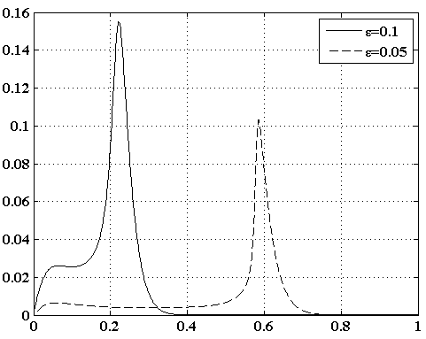
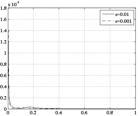
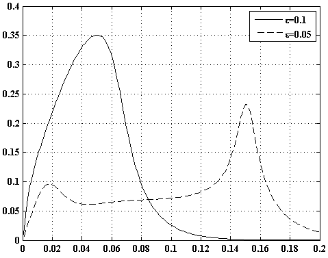
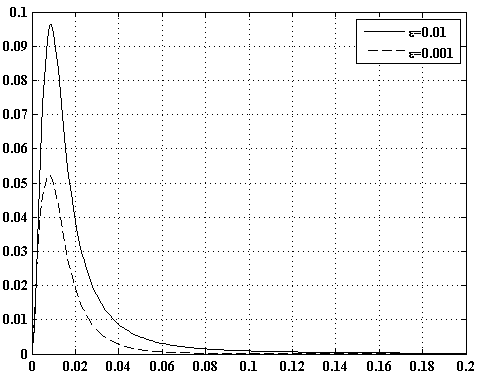
Figure 5. Evolution in time of the kinetic energy for $\varepsilon=0.1,0.05,0.01,0.001$. Top figures are for the two singularities experiment, meanwhile, bottom figures are for the four singularities experiment. In this case, we consider $M=2.0$.

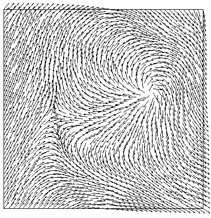
(a) $\|{\boldsymbol{d}}\|_{\infty}=1.11139$

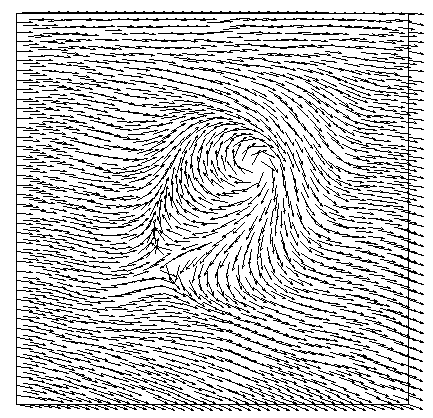
(b) $\|{\boldsymbol{d}}\|_{\infty}=1.01984$

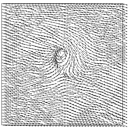
(c) $\|{\boldsymbol{d}}\|_{\infty}=1.06926$

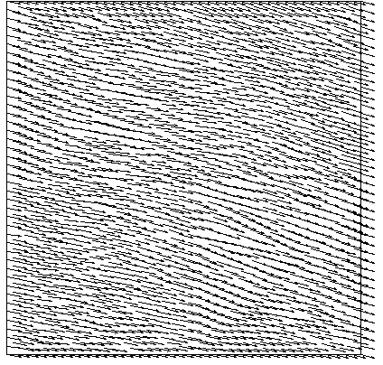
(d) $\|{\boldsymbol{d}}\|_{\infty}=0.992742$

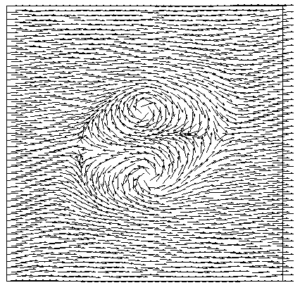
(e) $\|{\boldsymbol{d}}\|_{\infty}=1.04313$

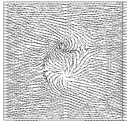
(f) $\|{\boldsymbol{d}}\|_{\infty}=1.06166$

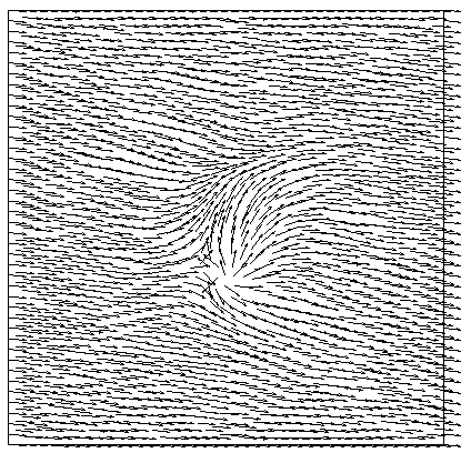
(g) $\|{\boldsymbol{d}}\|_{\infty}=1.03869$

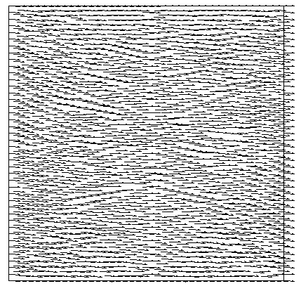
(h) $\|{\boldsymbol{d}}\|_{\infty}=1$

Figure 6. Evolution of the director field for a rotating flow. Top figures: two singularities experiment at times $t=0.2,0.5,2.0,3$. Bottom figures: four singularities experiment at times $t=0.1,0.6,1.3,3$.

References

- [1] S. Badia. On stabilized finite element methods based on the Scott-Zhang projector. Circumventing the inf-sup condition for the Stokes problem. Comput. Methods Appl. Mech. Engrg. 247/248 (2012), 65-72.
- [2] S. Badia, F. Guillén-Gonzalez, J. V. Gutiérrez-Santacreu. Finite element approximation of nematic liquid crystal flows using a saddle-point structure. J. Comput. Phys. 230 (2011), no. 4, 1686-1706.
- [3] S. Badia, F. Guillén-Gonzalez, J. V. Gutiérrez-Santacreu. An overview on numerical analyses of nematic liquid crystal flows. Arch. Comput. Methods Eng. 18 (2011), no. 3, 285-313.
- [4] R. Becker, X. Feng, A. Prohl. Finite element approximations of the Ericksen-Leslie model for nematic liquid crystal flow. SIAM J. Numer. Anal. 46 (2008), no. 4, 1704-1731.
- [5] E. Burman, M.A. Fernández. Galerkin finite element methods with symmetric pressure stabilization for the transient Stokes equations: stability and convergence analysis, SIAM J. Numer. Anal. 47 (2008), no. 1, 409-439.
- [6] R.C. Cabrales, F. Guillén-González, J.V. Gutierrez-Santacreu. A time-splitting finite-element stable approximation for the Ericksen-Leslie equations. SIAM J. Sci. Comput., 37(2015), B261-B282.
- [7] R. Codina. Pressure stability in fractional step finite element methods for incompressible flows. J. Comput. Phys. 170 (2001), no. 1, 112-140.
- [8] J. Ericksen. Conservation laws for liquid crystals. Trans. Soc. Rheol., 5 (1961), 22-34.
- [9] J. Ericksen. Continuum theory of nematic liquid crystals. Res. Mechanica, 21 (1987), 381-392.
- [10] V. Girault, F. Guillén-González. Mixed formulation, approximation and decoupling algorithm for a nematic liquid crystals model. Math. Comput. 80 (2011), no. 274, 781-819.
- [11] J.-L. Guermond, P. Minev, J. Shen. An overview of projection methods for incompressible flows. Comput. Methods Appl. Mech. Engrg. 195 (2006), 6011-6045
- [12] F. Guillén-Gonzalez, J. V. Gutiérrez-Santacreu. A linear mixed finite element scheme for a nematic Ericksen-Leslie liquid crystal model. ESAIM: M2AN. 47 (2013), no. 5, 1433-1464.
- [13] F. Hecht. New development in freefem++. J. Numer. Math. 20 (2012), no. 3-4, 251-265.
- [14] Jeffery, G.B. The motion of ellipsoidal particles immersed in a viscous fluid. Roy. Soc. Proc. 102 (1922), 161-179.
- [15] F. Leslie. Theory of flow phenomena in liquid crystals. The Theory of Liquid Crystals. W. Brown, ed. Academic Press, New York, 4 (1979), 1-81.
- [16] F. Leslie. Some constitutive equations for liquid crystals. Arch. Ration. Mech. Anal., 28 (1968), 265-283.
- [17] P. Lin, C. Liu, H. Zhang. An energy law preserving finite element scheme for simulating the kinematic effects in liquid crystal flow dynamics. Journal of Computational Physics 227 (2007), 348-362.
- [18] C. Liu, J. Shen, X. Yang. Dynamics of Defect Motion in Nematic Liquid Crystal Flow: Modeling and Numerical Simulation. Commun. Comput. Phys. 2 (2007), 1184-1198.
- [19] C. Liu, N.J. Walkington. Mixed methods for the approximation of liquid crystal flows. M2AN Math. Model. Numer. Anal. 36 (2002), 205-222.
- [20] C. Liu, N.J. Walkington. Approximation of liquid crystal flows. SIAM J. Numer. Anal. 37 (2000), 725-741.
- [21] L. R. Scott, S. Zhang. Finite element interpolation of non-smooth functions satisfying boundary conditions. Math. Comp., 54, (1990), 483–493.
- [22] R. Temam. Navier-Stokes equations, theory and numerical analysis. AMS Chelsea Publishing, Providence, 2001.