Redshift Measurement and Spectral Classification
for eBOSS Galaxies with the redmonster Software

Abstract

We describe the redmonster automated redshift measurement and spectral classification software designed for the extended Baryon Oscillation Spectroscopic Survey (eBOSS) of the Sloan Digital Sky Survey IV (SDSS-IV). We describe the algorithms, the template standard and requirements, and the newly developed galaxy templates to be used on eBOSS spectra. We present results from testing on early data from eBOSS, where we have found a 90.5% automated redshift and spectral classification success rate for the luminous red galaxy sample (redshifts 0.6 $\lesssim$ $z$ $\lesssim$ 1.0). The redmonster performance meets the eBOSS cosmology requirements for redshift classification and catastrophic failures, and represents a significant improvement over the previous pipeline. We describe the empirical processes used to determine the optimum number of additive polynomial terms in our models and an acceptable $\Delta\chi_{r}^{2}$ threshold for declaring statistical confidence. Statistical errors on redshift measurement due to photon shot noise are assessed, and we find typical values of a few tens of km s^-1. An investigation of redshift differences in repeat observations scaled by error estimates yields a distribution with a Gaussian mean and standard deviation of $\mu\sim$ 0.01 and $\sigma\sim$ 0.65, respectively, suggesting the reported statistical redshift uncertainties are over-estimated by $\sim$ 54%. We assess the effects of object magnitude, signal-to-noise ratio, fiber number, and fiber head location on the pipeline’s redshift success rate. Finally, we describe directions of ongoing development.

1. Introduction

Redshift surveys are a fundamental tool in modern observational astronomy. These surveys aim to measure redshifts of galaxies, galaxy clusters, and quasars to map the 3-dimensional distribution of matter. These observations allow measurements of the statistical properties of the large-scale structure of the universe. In conjunction with observations of the cosmic microwave background, redshift surveys can also be used to place constraints on cosmological parameters, such as the Hubble constant (e.g., Beutler et al., 2011) and the dark energy equation of state through measurements of the baryon acoustic oscillation (BAO) peak, first detected in the clustering of galaxies (Eisenstein et al., 2005, Cole et al., 2005). The first systematic redshift survey was the CfA Redshift Survey (Davis et al., 1982), measuring redshifts for approximately 2,200 galaxies. Such early surveys were limited in scale due to single object spectroscopy. The development of fiber-optic and multi-slit spectrographs enabled the simultaneous observations of hundreds or thousands of spectra, making possible much larger surveys, such as the DEEP2 Redshift Survey (Newman et al., 2013), the 6dF Galaxy Survey (6dFGS; Jones et al., 2004), Galaxy and Mass Assembly (GAMA; Liske et al., 2015), and the VIMOS Public Extragalactic Survey (VIPERS; Garilli et al., 2014), measuring redshifts for approximately 50,000, 136,000, 300,000, and 55,000 objects, respectively.

The Sloan Digital Sky Survey (SDSS; York et al., 2000) is the largest redshift survey undertaken to date. At the conclusion of SDSS-III, the third iteration of SDSS (Eisenstein et al., 2011), a total of 4,355,200 spectra had been obtained. Of these, 2,497,484 were taken as part of the Baryon Oscillation Spectroscopic Survey (BOSS; Dawson et al., 2013), containing 1,480,945 galaxies, 350,793 quasars, and 274,811 stars. The “constant mass” (CMASS) subset of the BOSS sample is composed of massive galaxies over the approximate redshift range of $0.4<z<0.8$ and typical S/N values of $\sim 5$/pixel. The automated redshift measurement and spectral classification of such large numbers of objects presents a challenge, inspiring refinements of the spectro1d pipeline (Bolton et al., 2012). This software models each co-added spectrum as a linear combination of principal component analysis (PCA) basis vectors and polynomial nuisance vectors and adopts the combination that produces the minimum $\chi^{2}$ as the output classification and redshift. PCA-reconstructed models were chosen due to their close ties to the data, allowing the PCA eigenspectra to potentially capture any intrinsic populations within the training sample. This pipeline was able to achieve an automated classification success rate of 98.7% on the CMASS sample (and 99.9% on the lower-redshift, higher-S/N LOWZ sample). However, the software was only able to successfully classify 79% of the quasar sample, which resulted in the need for the entire sample to be visually inspected (Pâris et al., 2012).

The Sloan Digital Sky Survey IV (SDSS-IV; Blanton et al., 2016) is the fourth iteration of the SDSS. Within SDSS-IV, the Extended Baryon Oscillation Spectroscopic Survey (eBOSS; Dawson et al., 2016) will precisely measure the expansion history of the Universe throughout eighty percent of cosmic time through observations of galaxies and quasars in a range of redshifts left unexplored by previous redshift surveys. Ultimately, eBOSS plans to use approximately 300,000 luminous red galaxies (LRGs; 0.6 $<$ $z$ $<$ 1.0), 200,000 emission line galaxies (ELGs; 0.7 $<$ $z$ $<$ 1.1), and 700,000 quasars (0.9 $<$ $z$ $<$ 3.5) to measure the clustering of matter.

The primary science goal of eBOSS is to measure the length scale of the BAO feature in the spatial correlation function in four discrete redshift intervals to $1-2$% precision, thereby constraining the nature of the dark energy that drives the accelerated expansion of the present-day universe. A set of requirements for the redshift and classification pipeline was established to meet these goals. As given in Dawson et al. (2016), these requirements are: (1) redshift accuracy $c\sigma_{z}/(1+z)<$ 300 km s^-1 for all tracers at redshift $z<1.5$ and $<(300+400(z-1.5))$ km s^-1 RMS for quasars at $z>1.5$ ; and (2) fewer than 1% unrecognized redshift errors of $>1000$ km s^-1 for LRGs and $>3000$ km s^-1 for quasars (referred to in this paper as “catastrophic redshift failures”). Additionally, the pipeline should return confident redshift measurements and classifications for $>90$% of spectra.

The higher-redshift, lower-S/N (typically $\sim 2$/pixel for galaxies) targets in eBOSS present a new challenge for automated redshift measurement and classification software. Initial tests with the spectro1d PCA basis vectors predicted success rates of $\sim 70$% for the LRG sample, which is well below the specified science requirements. This is due, in part, to the flexibility in fitting PCA components to a spectrum, which allows non-physical combinations of basis vectors to pollute the redshift measurements and statistical confidences thereof. Additionally, while possible (e.g., Chen et al., 2012), mapping PCA coefficients onto physical properties is a difficult task. It requires the use of a transformation matrix, and confidence in the results is, at best, unintuitive, and possibly uncertain.

To meet these challenges, we have developed an archetype-based software system for redshift measurement and spectral classification named redmonster. We have developed a set of theoretical templates from which spectra can be classified. redmonster is written in the Python programming language. The project is open source, and is maintained on the first author’s GitHub account. The analysis performed in this paper uses tagged version v1_0_0. The development of this software was driven by the following goals:

1. Redshift measurement and classification on the basis of discrete, non-negative, and physically-motivated model spectra;

2. Robustness against unphysical PCA solutions likely to arise for low-S/N ELG and LRG spectra in eBOSS, particularly in the presence of imperfect sky-subtraction;

3. Determination of joint likelihood functions over redshift and physical parameters;

4. Self-consistent determination and application of hierarchical redshift priors;

5. Self-consistent incorporation of photometry and spectroscopy in performing redshift constraints;

6. Simultaneous redshift and parameter fits to each individual exposure in multi-exposure data;

7. Custom configurability of spectroscopic templates for different target classes;

8. Automated identification of multi-object superposition spectra.

The software as described in this paper meets design goals 1, 2, 3, and 7. We have chosen to enumerate the full list of design goals to provide a forward-looking vision of new and interesting possibilities.

In this paper, we describe redmonster and its application to the eBOSS LRG sample. The organization is as follows: Section 2 describes automated redshift and classification algorithms and procedures of redmonster. We include the requirements and standardized format for templates and a description of the eBOSS galaxy and star templates in Section 2.1. The core redshift measurement algorithm is described in Section 2.2 and Section 2.3. Section 3 gives an overview of the spectroscopic data sample of eBOSS and an analysis of the tuning and performance of the software on eBOSS data, including completeness and purity. Section 4 provides a description of the classification of eBOSS LRG spectra, including redshift success dependence, effects on the final redshift distribution in eBOSS, and precision and accuracy. Finally, Section 5 provides a summary and conclusion. The content and structure of the output files of redmonster are described in Appendix A.

2. Software Overview

The use of physically-motivated templates allows mapping of physical properties from the best-fitting template onto the model used to create the suite of templates. To better facilitate the exploration of large, multi-dimensional parameter spaces, spectral fitting is performed in Fourier space, allowing redmonster to combine the speed of cross-correlation techniques with the statistical framework of forward-modeling. Additionally, significant effort has been made to write software not specific solely to SDSS, but rather in a manner that facilitates use in other redshift surveys, such as the Dark Energy Spectroscopic Instrument (DESI; Levi et al., 2013). We have also prioritized end-user customizability in the way the software operates.

Informed by our design goal of developing survey-agnostic software, the current version of redmonster requires only the following data as input:

1. Wavelength-calibrated, sky-subtracted, flux-calibrated, and co-added spectra, rebinned onto a uniform baseline of constant $\Delta$log${}_{10}\lambda$ per pixel;

2. Statistical error-estimate vectors for each spectrum, expressed as inverse variance.

While SDSS spectra are shifted such that measured velocities will be relative to the solar system barycenter at the mid-point of each 15-minute exposure, no such requirement exists for redmonster input spectra. Redshifts will be measured relative to a frame of the end-user’s choosing.

2.1. Templates

In order to make redshift and parameter measurements and select among galaxy, quasar, and stellar (and possibly other) object types with the highest statistical confidence, the pipeline requires a set of templates that both spans the entire space of object types within the survey and covers the full wavelength range of the spectrograph over the redshift range of interest. To this end, redmonster uses “archetype” template grids, where “archetype” refers to single spectral templates that are not fit in linear combination with any other templates, excluding low-order polynomial nuisance vectors. A series of archetype spectral templates spanning the relevant parameter space is recorded in an ndArch.fits (signifying N-dimensional archetypes) file. These ndArch.fits files conform to a standard that requires a general form of template spectra written by end users and ingested into the redshift software. The format allows highly configurable spectroscopic template classes without any re-coding of the low-level fitting routines. This file standard is oriented towards the familiar units and conventions of optical spectroscopic redshift measurement. Reader and writer routines for ndArch.fits files conforming to this standard are included in the redmonster package. A brief description of the standard is given here, while full documentation can be found in the software package.

The data contained in an ndArch.fits file consists of a single multi-dimensional array that contains all possible spectral templates for a class of object, containing flux densities or luminosity densities in units of $F_{\lambda}$ (power per unit area per unit wavelength) or $L_{\lambda}$ (power per unit wavelength). The absolute normalization may be physically meaningful, but is not required to be so. The first axis of the data array corresponds to vacuum wavelength and is gridded in positive increments of constant $\log\lambda$.

There may be one or more axes in addition to the first axis, up to the maximum number allowed by the FITS standard. Each axis beyond the first will generally correspond to a monotonically ordered physical model-parameter dimension (age, metallicity, emission-line strength, etc.), but may also correspond to an arbitrary labeled or unlabeled collection. The archetype template vectors are assumed to have a uniform resolution characterized by a Gaussian line-spread function with a dispersion parameter $\sigma$ equal to one sampling pixel.

Templates are segregated into template classes, with each class corresponding to a single object type of interest and contained in a single ndArch.fits file. These classes are used by redmonster to classify the object type of a given spectrum. Three template classes have been developed for use in the eBOSS pipeline. Galaxy templates for LRG targets are described in §2.1.1. Quasar and stellar templates have been developed and are included with redmonster. Because this paper focuses primarily on performance of redmonster spectroscopic classifications on the eBOSS LRG target sample, these templates function primarily to identify non-galaxy objects that arise due to targeting impurities. As such, we defer description of quasar and stellar templates to a later work.

2.1.1 Galaxy templates

Our LRG templates are selected from the Flexible Stellar Population Synthesis (FSPS) model suite (Conroy et al., 2009, Conroy & Gunn, 2010) with the Padova isochrones (Marigo et al., 2008) and a Kroupa IMF (Kroupa, 2001). The spectra used in the models are custom high resolution theoretical spectra (Conroy, Kurucz, Cargile, Castelli,, in prep.); the resulting models are referred to as FSPS-C3K. The synthetic spectral library was constructed with the latest set of atomic and molecular line lists (courtesy of R. Kurucz) and is based on the Kurucz suite of spectral synthesis and stellar atmosphere routines (SYNTHE and ATLAS12; Kurucz, 1970, Kurucz, 1993; Kurucz & Avrett, 1981). The grid of spectra was computed assuming the Asplund et al. (2009) solar abundance pattern and a constant microturbulence of 2 km s^-1. For further details see Conroy & van Dokkum (2012a). Table 1 lists the physical parameters of the LRG template suite, their range, and the frequency with which they are binned. All models are solar metallicity. Several example templates are shown in Figure 1. The templates have been vertically offset by 800, 600, 400, 250, and 100 for visual clarity. The wavelength range of the BOSS spectrograph extends from $3600$ Å to $1.04\ \mu$m, while the templates span the range $1525$ Å $<\lambda<10852$ Å, allowing the templates to span the redshift range $0<z<1.36$. These templates will be extended further into the blue to cover the full redshift range of the ELG sample in SDSS DR14.

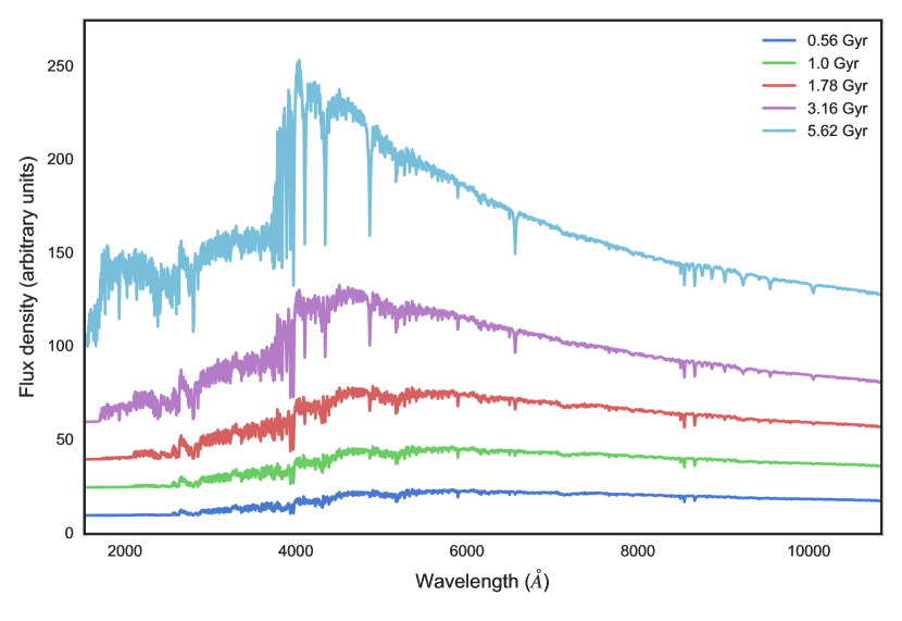
Figure 1.— Example LRG templates of various ages. The templates have been vertically offset for increased visibility.

Table 1 Galaxy template physical parameter dimensions and sampling

Parameter	Range	$N_{samples}$
$\log_{10}\mathrm{(Age)}$	[-2.5, 1] Gyr	15
$\log_{10}\sigma_{vel}$	[2, 2.6] km s-1	4
H$\alpha$ EW	[0, 100] Å	5

2.1.2 Stellar templates

Our stellar templates are synthetic spectra computed using Kurucz ATLAS9 models by Mészáros et al. (2012) and the radiative transfer code ASS$\epsilon$T (Koesterke, 2009). The reference solar abundances are from Asplund et al. (2005), with enhanced $\alpha$-element abundances, mimicking the trends found in the Milky Way, and a constant micro-turbulence velocity of 2 km s^-1. Continuum opacity is based on the Opacity Project and Iron Project photoionization cross-sections, collected by Allende Prieto et al. (2003) and Allende Prieto (2008), and line opacities are based on data compiled by Kurucz, with updates from Barklem et al. (2000). Line absorption coefficients for Balmer lines are computed with the codes provided by Barklem & Piskunov (2015).

2.2. Spectral fitting

The redmonster software approaches redshift measurement and classification as a $\chi^{2}$ minimization problem by cross-correlating the observed spectrum with each spectral template in the ndArch.fits file over a discretely sampled redshift interval. The algorithm is similar to the method described by Tonry & Davis (1979). By default, pixels with S/N $>200$ (which likely indicates a cosmic ray) or with $f_{\lambda}<-10\sigma$ (unphysical negative flux at $10\sigma$ significance), are masked for each observed spectrum. These values are configurable when running the software. The spectrum is then fit with an error-weighted least-squares linear combination of a single template and a low-order polynomial across the range of trial redshifts. The polynomial term serves to absorb Galactic and intrinsic interstellar extinction, sky-subtraction residuals, and spectro-photometric calibration errors not accounted in the templates. By default, trial redshifts are separated by the spacing set by a single pixel in wavelength, though this, too, is configurable. For the eBOSS classifications, we have chosen to separate trial redshifts by one pixel for stars, two pixels for galaxies, and four pixels for quasars ($\sim 69$ km s^-1, $\sim 138$ km s^-1, and $\sim 278$ km s^-1, respectively) to reduce computation time. A redshift range must also be specified for each ndArch.fits file being used; for the eBOSS data, we use $-0.1<z<1.2$ for galaxies, $-0.005<z<0.005$ for stars, and $0.4<z<3.5$ for quasars. This fitting process results in a $\chi^{2}$ value for a spectral template at a single trial redshift. Repeating this fit for all templates within the ndArch.fits and across all trial redshifts defines a $\chi^{2}(\vec{P},z)$ surface, where $\vec{P}$ is a vector spanning the parameter-space of the template class.

The software is able to explore large parameter spaces within a template class by pre-computing some matrix elements in Fourier space during the fitting process (see also Glazebrook et al., 1998). In order to fit a set of data $\vec{d}$ with a set of $n$ basis vectors $\{\vec{x}_{k}\}$ in a minimum $\chi^{2}$ sense, the model $\vec{m}$ takes the form

$$\vec{m}=\sum\limits_{k=1}^{n}a_{k}\vec{x}_{k},$$ (1)

where, in the case of redmonster, $\{\vec{x}_{k}\}$ consists of a single physical template and $n-1$ polynomial terms. Thus, the $\chi^{2}$ of the model relative to the data, assuming $N$ data points, is

$$\chi^{2}=\sum\limits_{i=1}^{N}\frac{(d_{i}-\sum\limits_{k=1}^{n}a_{k}x_{k,i})^{2}}{\sigma_{i}^{2}}$$ (2)

where $\sigma_{i}^{2}$ is the statistical variance of the $i^{\mathrm{th}}$ pixel of $\vec{d}$. We find the $j^{\mathrm{th}}$ maximum likelihood estimator, $\hat{a}_{j}$, by minimizing $\chi^{2}(\vec{a})$ with respect to $a_{j}$. Here, $a_{j}$ is an arbitrarily chosen basis vector coefficient from $\vec{a}$, as the result is independent of our choice. Solving $\partial{\chi^{2}}/\partial{a_{j}}~{}=~{}0$ yields

$$\sum\limits_{i=1}^{N}\sum\limits_{k=1}^{n}\frac{\hat{a}_{k}x_{k,i}x_{j,i}}{\sigma_{i}^{2}}=\sum\limits_{i=1}^{N}\frac{d_{i}x_{j,i}}{\sigma_{i}^{2}}.$$ (3)

Because eBOSS spectra are binned linearly in $\mathbf{\log_{10}}\lambda$, velocity redshifts are uniform linear shifts in pixel space. Thus, fitting at a trial redshift introduces a “lag” in pixel-space $l$ of the basis vectors relative to the data, after which estimators become a function of $l$, and Eq. 3 becomes

$$\sum\limits_{i=1}^{N}\sum\limits_{k=1}^{n}\frac{\hat{a}_{k}(l)x_{k,i-l}x_{j,i-l}}{\sigma_{i}^{2}}=\sum\limits_{i=1}^{N}\frac{d_{i}x_{j,i-l}}{\sigma_{i}^{2}}.$$ (4)

This result can be cast in terms of matrices:

$$(\textbf{P}^{\top}\textbf{N}^{-1}\textbf{P})\vec{\hat{a}}=(\textbf{P}^{\top}\textbf{N}^{-1})\vec{d}$$ (5)

where P is an $(N\times n)$ matrix with each column a basis vector, N is an $(N\times N)$ diagonal matrix with $\textbf{N}_{ii}=$ $\sigma_{i}^{2}$, and $\vec{\hat{a}}$ is the vector of maximum likelihood esimators for which we wish to solve. The product $\textbf{P}^{\top}\textbf{N}^{-1}\textbf{P}$ is the correlation matrix of the templates, with elements

$$(\textbf{P}^{\top}\textbf{N}^{-1}\textbf{P})_{jk}=\sum\limits_{i=1}^{N}\frac{x_{j,i-l}x_{k,i-l}}{\sigma_{i}^{2}},$$ (6)

while the elements $(\textbf{P}^{\top}\textbf{N}^{-1}\vec{d})_{jk}$ are given by the right-hand side of Eq. 4. Over a range of continuous $l$, these elements are the discrete convolutions $(1/\vec{\sigma^{2}})*(\vec{x}_{j}\cdot\vec{x}_{k})(l)$ and $(\vec{d}/\vec{\sigma^{2}})*\vec{x_{j}}(l)$, respectively, and may be computed as products in Fourier space. Since the polynomial terms have no physical meaning, they may remain fixed in the observed frame of the data (i.e., have no $l$ dependence), and it is possible to pre-compute the fraction $(n-1)^{2}/n^{2}$ of the total matrix elements for a template class, greatly reducing computational requirements.

One of the motivations for the development of redmonster and its galaxy templates was the restriction that all redshifts and classifications must be derived from physical models. To that end, the resulting $\hat{a}_{k}(l)$ at each point in redshift-parameter space is evaluated for physicality based on the coefficient of the template component of the model. Fits with a negative template amplitude are rejected, and that point in the $\chi^{2}(\vec{P},z)$ surface is assigned a value of $\chi_{\mathrm{null}}^{2}$, where $\chi_{\mathrm{null}}^{2}$ is defined as the $\chi^{2}$ of the best-fit model where the amplitude of the template coefficient is forced to 0 (i.e., a polynomial-only model). Because the best-fit models produce the lowest possible $\chi^{2}$ value at each point in redshift-parameter space, and because the value of $\chi_{\mathrm{null}}^{2}$ is a function only of the data itself, the effect of this physicality constraint is to introduce a flat “ceiling” in the $\chi^{2}(\vec{P},z)$ surface, while maintaining continuity.

Table 2 redmonster ZWARNING bit-mask definitions

Bit	Name	Definition
0	SKY	Sky fiber
1	LITTLE_COVERAGE	Insufficient wavelength coverage
2	SMALL_DELTA_CHI2	$\chi^{2}$ of best fit is too close to that of second best ($<0.01$ in $\chi_{r}^{2}$)
5	Z_FITLIMIT	$\chi_{\mathrm{min}}^{2}$ at edge of the redshift fitting range (Z_ERR set to -1)
7	UNPLUGGED	Fiber was broken or unplugged, and no spectrum was obtained
8	NULL_FIT	At least one template class had constant-valued $\chi^{2}$ surface

2.3. $\chi^{2}$ interpretation

After the computation of the $\chi^{2}(\vec{P},z)$ surface for each template class, the minimum $\chi^{2}$ in spanning all templates is found at each trial redshift. The resulting series of best fits defines a $\chi^{2}(z)$ curve for each template class (similar to Figure 2 of Bolton et al., 2012). Interpolation over this curve is then performed using a cubic B-spline (i.e., a C2-continuous composite Bézier curve), through which all local minima are identified. The $N$ best redshifts for a particular template class are defined by the $N$ lowest minima of the $\chi^{2}(z)$ curve. The curve around each of these minima is then fit by a quadratic function using the three points nearest the minimum. The analytic minima of each quadratic fit are adopted as the spectrum’s candidate redshifts. The statistical error on each candidate is evaluated as the change in redshift $\pm\delta z$ for which the $\chi^{2}$ of the quadratic fit increases by one from its minimum value.

In the event the global minimum falls on the edge of the explored redshift range, the Z_FITLIMIT bit is triggered within the ZWARNING bit-mask, and both Z and Z_ERR are set to -1. The definitions of all failure modes captured by ZWARNING are shown in Table 2. Bit-masks 0-7 are identical to those of spectro1d, although bits 3, 4 and 6 are not used by redmonster and are retained only for consistency. Bit 4 (MANY_OUTLIERS) was found in SDSS-III to flag too many good quasar redshifts. Bit 6 (NEGATIVE_EMISSION) has been deprecated, allowing all spectra to be considered. The NEGATIVE_MODEL bit (bit 3) is unnecessary as redmonster restricts the template amplitude to be positive for reasons of physicality. Bit 8 is new and is triggered in the rare case of a template class having a $\chi^{2}$ surface with no local minima. The output files are discussed in detail in Appendix A.

Due to noise, some spectra can have multiple minima in the vicinity of one another that are not statistically significant. For all template classes, we ignore local minima that are separated in redshift from a lower-$\chi^{2}$ minimum by less than a given threshold, $\Delta$V. Local minima separated by more than $\Delta$V are explicitly evaluated, since they constitute redshift failures if they are statistically indistinguishable from one another. We define a quantity, $\Delta\chi_{\mathrm{threshold}}^{2}$, as the minimum acceptable $\Delta\chi_{\mathrm{red}}^{2}=(\chi_{2}^{2}-\chi_{1}^{2})/$dof, where $\chi_{1}^{2}$ corresponds to the global minimum and $\chi_{2}^{2}$ corresponds to some secondary minimum. The $\Delta\chi_{\mathrm{red}}^{2}$ between two minima must be greater than this threshold for statistical confidence to be declared. Values of $\Delta\chi_{\mathrm{red}}^{2}$ less than this threshold will trigger the SMALL_DELTA_CHI2 bit in the ZWARNING bit-mask, indicating a lack of statistical confidence. This process is illustrated schematically in Figure 2 of Bolton et al. (2012); example $\chi^{2}(z)$ curves from eBOSS spectra are shown in Figure 2.

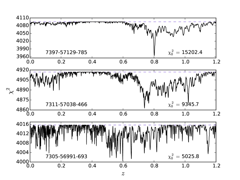
Figure 2.— Example $\chi^{2}(z)$ curves from the fits to spectra of three different LRG targets. The spectra are labeled by PLATE-MJD-FIBERID. The dashed purple lines show the value of $\chi_{\mathrm{null}}^{2}$. The $\chi_{0}^{2}$ values shown are the $\chi^{2}$ of a $\vec{0}$ model (i.e., the (S/N)² of the data). Note that the vertical axis shows raw $\chi^{2}$, and must be scaled by the number of degrees of freedom (i.e., the number of unmasked spectrum pixels minus the number of components in the fit) for comparison with $\Delta\chi_{\mathrm{threshold}}^{2}$. The top panel shows a $z=0.802$ galaxy with ZWARNING $=0$, indicating a confident redshift measurement and classification. The middle panel shows an LRG target with statistically indistinguishable fits at $z=0.738$ and $z=1.021$, triggering the SMALL_DELTA_CHI2 flag (ZWARNING $=4$). The bottom panel shows an LRG target with no $\chi^{2}$ minima separated from $\chi_{\mathrm{null}}^{2}$ with significance greater than $\Delta\chi_{\mathrm{threshold}}^{2}=0.005$.

The fits are then compared across template classes if multiple ndArch files were used. The $N$ best fits from each template class are combined into a single set, and are then sorted in ascending order of $\chi_{\mathrm{{red}}}^{2}$. The $N$ best fits from this combined set are adopted as the best redshifts and classifications for the object. These fits are re-evaluated for statistical confidence and flagged according to the above criteria, although $\chi_{\mathrm{min}}^{2}$ separated by less than $\Delta$V will no longer trigger the SMALL_DELTA_CHI2 flag. Additionally, redshift differences between two classes less than the quadrature sum of the error estimates are not flagged even if the $\Delta\chi^{2}$ is below the threshold, as the redshift, and not the class, is the primary measurement being made. By default, the software keeps five redshifts and classifications per spectrum ($N=5$), but this is user-configurable.

We note here that, strictly speaking, the use of minimium-$\chi^{2}$ regression should be limited to cases where the measurement errors account for all of the statistical scatter and the model is correctly specified (i.e., the template class is correct). Otherwise, the parameter values and their confidence intervals may not be scientifically meaningful. While the measurement errors of eBOSS data do not account for all of the scatter and the chosen template family is not a complete representation of the galaxies present in the sample, we empirically calibrate the robustness of our statistics through the use of repeat observations, as discussed in §4.3.

3. Optimization of redmonster parameters for eBOSS LRGs

The main targets for eBOSS spectroscopy consist of LRGs at redshifts $0.6<z<1.0$ (Prakash et al., 2015), ELGs in the range $0.6<z<1.1$ (Comparat et al., 2015, Raichoor et al., 2016, Delubac et al., 2016), “clustering” quasars in the range $0.9<z<2.2$, re-observations of faint Ly$\alpha$ quasars in the range $2.1<z<3.5$, and new Ly$\alpha$ quasars at redshifts $2.1<z<3.5$ (Myers et al., 2015). A selection of example eBOSS spectra is shown in Figure 3. The spectral classification and redshift software described here will be applied to all spectra obtained with the BOSS spectrograph, including targets outside the LRG, ELG, and quasar selection algorithms. Here we demonstrate the tuning of redmonster parameters and the performance of redmonster on the LRG target sample from eBOSS.

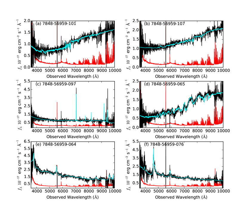
Figure 3.— Example eBOSS spectra. The data, smoothed over a 5-pixel window, are presented in black, the best-fit model from redmonster is shown in cyan, and the 1-$\sigma$ error (as estimated by idlspec2d) is shown in red. Each spectrum has been labeled with its unique PLATE-MJD-FIBERID. The objects shown here are: (a) LRG-target galaxy, $z=0.664$; (b) LRG-target galaxy, $z=0.943$; (c) ELG-target galaxy, $z=0.891$; (d) M-star; (e) quasar, $z=0.978$; (f) quasar, $z=2.823$.

The LRG target class consists of massive red galaxies that have been color-selected using SDSS imaging (Gunn et al., 1998) in ugriz filters (Fukugita et al., 1996) and imaging from the Wide-field Infrared Survey Explorer (WISE; Wright et al., 2010). These targets have a faint magnitude limit of $i<21.8$ (AB). A full investigation of the LRG selection is presented in Prakash et al. (2015).

Spectroscopic data for eBOSS are obtained using the 2.5-m Sloan Telescope at Apache Point Observatory (Gunn et al., 2006) with the BOSS spectrograph system. The BOSS instrument is composed of two double-arm spectrographs fed by 1000 optical fibers plugged into a drilled aluminum plate that is positioned in the telescope focal plane. A summary of this system is given in Table 2 of Bolton et al. (2012) and a full account is given in Smee et al. (2013). Each of the optical fibers feeding the spectrographs is numbered with a FIBERID index ranging from 1-1000. Each physical plug plate is given a unique PLATE number. Finally, because a given PLATE may be observed more than once with different mappings between FIBERID and target spectra, each plugging is given an MJD number corresponding to the modified Julian date of the observation. Thus, any combination of PLATE, MJD, and FIBERID constitutes a unique eBOSS co-added spectrum. Pluggings are observed in 15-minute exposures, which are co-added during the data reduction process as described in Dawson et al. (2013). The 1D spectral outputs of this calibration, extraction, and co-addition process are stored in the “spPlate” FITS files, which become the inputs to the software described in this paper.

Two significant changes have been made to the spectral extraction and co-addition of individual exposures for the second data release (DR14) of SDSS-IV. These changes were developed to improve classification of lower signal-to-noise data in eBOSS. The first major change improves the way atmospheric differential refraction (ADR) corrections are applied to eBOSS spectra, and is described in Jensen et al. (2016). The improved ADR corrections are similar to prior work (Margala et al., 2015, Harris et al., 2016) and primarily improve flux calibrations for quasar spectra. The second change corrects a known bias in the co-addition of individual exposures. This correction has significant impact on the classification of galaxy spectra; thus, we provide a description below.

Individual exposures are initially flux calibrated with no constraint that the same object has the same flux across different exposures. Empirical “fluxcorr” vectors are broadband corrections to bring the different exposures into alignment for each object prior to co-addition. In DR13 and prior, these were implemented for each spectrum by minimizing

$$\chi^{2}_{i}=\sum_{\lambda}{(f_{i\lambda}-f_{\mathrm{ref},\lambda}/a_{i\lambda})^{2}\over(\sigma_{i\lambda}^{2}+\sigma_{\mathrm{ref},\lambda}^{2}/a_{i\lambda}^{2})}$$ (7)

where $f_{i\lambda}$ is the flux of exposure $i$ at wavelength $\lambda$, $f_{\mathrm{ref},\lambda}$ is the flux of the selected reference exposure, and $a_{i\lambda}$ are low order Legendre polynomials. The number of polynomial terms is dynamic, up to a maximum of 5 terms. Higher order terms are added only if they improve the $\chi^{2}$ by 5 compared to one less term. This approach is biased toward small $a_{i\lambda}$ since that inflates the denominator to reduce the $\chi^{2}$.

For DR14, we solve the fluxcorr vectors relative to a common weighted co-add $F_{\lambda}$ which is treated as noiseless compared to the individual exposures,

$$\chi^{2}_{i}=\sum_{\lambda}{(f_{i\lambda}-F_{\lambda}/a_{i\lambda})^{2}\over\sigma_{i\lambda}^{2}}.$$ (8)

We additionally include an empirically tuned prior that $a_{i\lambda}\sim 1$ to avoid large excursions in the solution for very low signal-to-noise data. Figure 4 shows the fluxcorr corrections for five exposures of 155 LRGs. The left panel shows the DR13 corrections, which have a large scatter and average value less than one due to biased fluxcorr. The right panel shows the new algorithm in DR14, which reduces scatter and gives the corrections a mean close to unity.

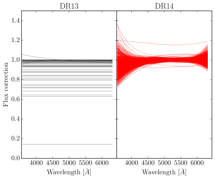
Figure 4.— Calibration corrections for 5 exposures of 155 LRG spectra on plate 7898 (blue camera) in DR13 (left panel) and DR14 (right panel).

Due to the highly configurable nature of redmonster, several input values must be determined for each unique data set to optimize performance. In this section, we demonstrate the optimization of the most influential, interesting, and challenging of those: $\Delta\chi_{\mathrm{threshold}}^{2}$ and the degree of the polynomial, $n_{\mathrm{poly}}$ to be fit in linear combination with the templates. A third important parameter to be determined is $\Delta V$, the half-width of the window around a $\chi^{2}$-minimum in which secondary minima are ignored. This was chosen for eBOSS as 1000 km s^-1 based on clustering science requirements, and thus will not be discussed here.

In order to explore the effects of these parameters and quantify performance of the software on galaxy spectra, we analyze the eBOSS LRG target sample, containing 99,449 unique observations of LRG targets. We use reductions produced by the tagged version v5_10_0 of the idlspec2d pipeline that will be released in DR14. Determination of the configurable $n_{\mathrm{poly}}$ is described in §3.1, and that of $\Delta\chi_{\mathrm{threshold}}^{2}$ in §3.2.

3.1. Determination of $n_{\mathrm{poly}}$

The number of additive polynomial terms fit in linear combination with the template spectrum can have a large impact on the quality of the fits and, thus, the failure rate and redshift errors. Some polynomial terms are necessary to absorb broad-band spectrophotometric calibration errors and astrophysical signal not reflected in the templates. Allowing too much freedom to the polynomial terms (i.e., too high an order) will allow them to fit real astrophysical features. Shifting the quality of the fit to the non-physical components of the model reduces the ability of the physical templates to provide statistically distinguishable fits to the data, thus increasing failure rates. In order to understand the effects of $n_{\mathrm{poly}}$, we processed the LRG sample with redmonster four separate times, using each of a constant, linear, quadratic, and cubic polynomial, producing a unique output file for each.

First, we computed the failure rate for each degree of polynomial. In all cases, the ZWARNING flag corresponding to SMALL_DELTA_CHI2 dominates the redshift failure modes. The failure rates for a constant, linear, quadratic, and cubic polynomial were 9.5%, 20.9%, 14.2%, and 12.9%, respectively. Additionally, we computed the distribution of $\Delta\chi^{2}$ per degree of freedom for each run, shown in Figure 5. The use of a constant polynomial term stands out as having both the lowest failure rate ($\sim 9.5\%$), and a systematic shift in the $\Delta\chi^{2}/\mathrm{dof}$ distribution toward higher values.

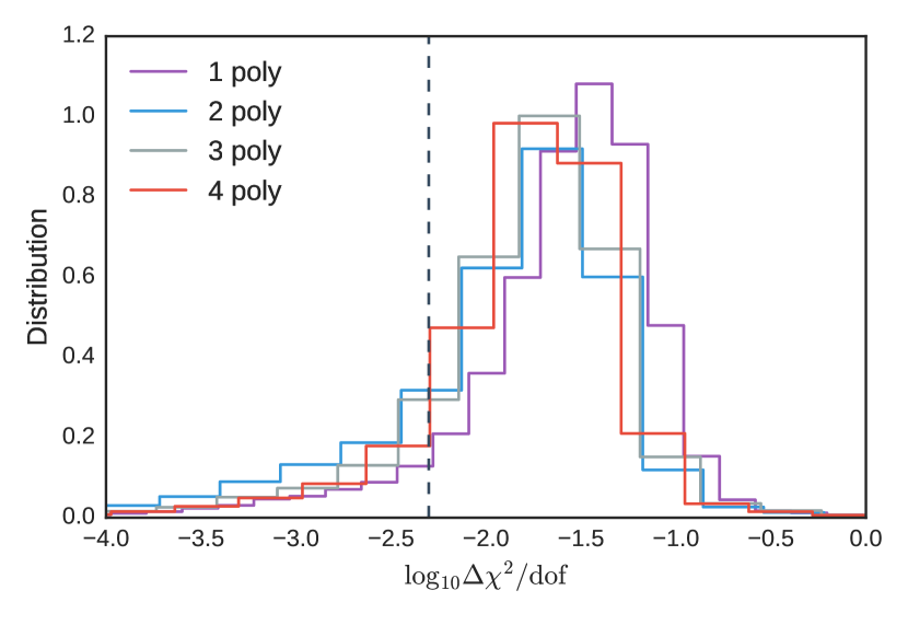
Figure 5.— Distribution of $\Delta\chi^{2}$ per degree of freedom of eBOSS LRGs for several orders of polynomial terms. The dashed vertical line represents a $\Delta\chi^{2}_{\mathrm{threshold}}$ cutoff of 0.005.

In order to understand how the order of the polynomial affects our best-fit models and their distinguishing power, we focus on the two candidates with the lowest failure rates - constant and cubic.

Figure 6 shows object-matched comparisons of several statistics of our fits for the constant- and cubic-order polynomials. We have highlighted cases where one of the models returned a successful measurement (ZWARNING = 0) while the other failed. The top panel shows the value $\chi^{2}_{\mathrm{null}}$ of each spectrum for both model types. All points lie to the right of the dashed line, meaning the constant-polynomial model absorbs less information from the spectrum than does the cubic-polynomial in every case. Further, the constant-polynomial has an RMS of $\sim$37,000, roughly 6.5 times larger than the RMS of the cubic-polynomial. The narrow range of values around $\chi_{\mathrm{null,4}}^{2}=4000-6000$ suggests the cubic-polynomial is consistently absorbing most of the broadband information, while the constant-polynomial often cannot. Meanwhile, the central plot, showing the minimum $\chi^{2}_{\mathrm{red}}$ for both models, shows a similar range of values for each. Thus, in the cases where the constant-polynomial component is unable to fit broadband information, the templates effectively take a significant fraction of the signal absorbed by the cubic-polynomial and transfer it to the physical template. The bottom panel of Figure 6 illustrates this further. The data show a linear relationship between the two values of $\Delta\chi^{2}/\mathrm{dof}$ with a slope of $<1$. On average, $\Delta\chi^{2}_{\mathrm{red}}$ is larger for the constant-polynomial model than for the cubic-polynomial model, consistent with the trend in Figure 5.

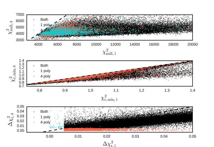
Figure 6.— Comparisons between several model-fit statistics on an object-by-object basis for a constant polynomial ($\chi_{~{},1}^{2}$) and cubic polynomial model ($\chi_{~{},4}^{2}$). The salmon and teal points correspond to objects where only the constant-polynomial and cubic-polynomial model returned a successful measurement, respectively. The dashed line shows the 1-to-1 line in each plot. Top: $\chi^{2}$ of polynomial-only model (i.e., no template component). Center: The $\chi^{2}/\mathrm{dof}$ of the polynomial + template combination that produces the best fit to the observed spectrum. Bottom: Difference in $\chi^{2}/\mathrm{dof}$ between best and second-best model.

Figure 7 shows $(\chi^{2}_{0}-\chi^{2}_{\mathrm{null}})/\chi^{2}_{0}$ of both polynomial choices for each object, where $\chi^{2}_{0}$ is the $\chi^{2}$ of a zero model (i.e, the (S/N)² of the data); thus, this quantity may be interpreted as the fraction of the total (S/N)² of the data absorbed by the polynomial. Note that all data points fall above the unity relationship, meaning the cubic polynomial always absorbs more of the information in the spectrum than does the constant. We have overlaid contours from a bivariate kernel density estimate, which has a maximum at (0.573, 0.831). The marginal plots show the univariate kernel density estimates for the constant polynomial on the horizontal axis and cubic polynomial on the vertical axis. The median values of the constant and cubic are 0.553 and 0.787, respectively, suggesting that, on average, the cubic polynomial and spectral template absorbs $\sim 23\%$ more, in absolute terms, of the spectrum’s signal than does the constant polynomial and spectral template.

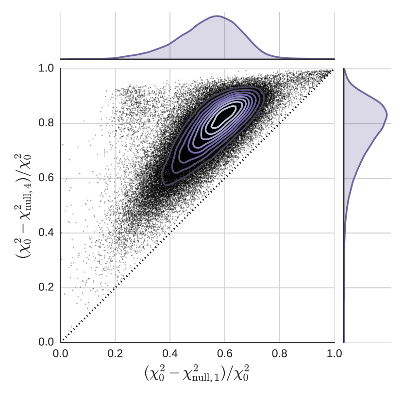
Figure 7.— Fraction of each object’s total (S/N)² absorbed by the polynomial-only model for a constant and cubic polynomial, with bivariate kernel density estimate overlaid. The dotted line shows the unity relationship. Marginal plots show univariate kernel density estimates for each axis.

As a final means of exploring the effects of changing the order of the polynomial, we visually inspected spectra which returned a successful measurement in one run but a failure in the other. The visual inspections help us to develop a qualitative understanding of the types of spectra or spectral features that are handled successfully in one case and are problematic for the other. Figure 8 shows a $z=0.743$ galaxy from the LRG sample for which the constant-polynomial model returned a successful redshift measurement and the cubic-polynomial model returned a failure. This spectrum was chosen as being representative of the typical behavior of models with constant-success and cubic-failure. There is a clear unphysical upturn in the noisy blue end of the spectrum due to calibration errors, which happens occasionally among low S/N eBOSS spectra. The higher flexibility of the cubic-polynomial fit allows the model to chase this upturn, which shifts power into the non-physical component of the model and away from the physical template. Because the long wavelength corrections are coupled to the short wavelength corrections through the cubic polynomial, this results in the suppression of the equivalent width of narrow-band features such as Ca H&K at 3968.5 and 3933.7 Å, respectively, H$\beta$ at 4863 Å, Mg I at 5175 Å, and Na I at 5894 Å. In low signal-to-noise spectra, such as those of eBOSS, it becomes difficult for the software to distinguish between the model fitting a real narrow-band feature and fitting noise. In this case, the cubic-polynomial model does, in fact, have the correct redshift, but due to reduced template amplitude relative to the constant-polynomial model, lacks the statistical confidence to declare a confident measurement.

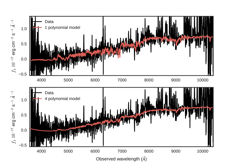
Figure 8.— Example of an object (PLATE 7572 MJD 56944 FIBERID 515) in which a constant-polynomial model returned a successful measurement while the cubic-polynomial measurement failed. The data are shown in black, and the best-fit model is shown in red.

On the other hand, for spectra with the largest broadband deviations from the templates or deviations that extend beyond the blue end (due to flux calibration errors, object superpositions, etc.), the constant-polynomial model lacks the flexibility to fit these features. In these cases, the $\chi^{2}$ is driven by poor fitting of the broadband features, and the relative contribution from the astrophysical features is small. This hinders the software’s ability to distinguish between models with different physical parameters. The cubic-polynomial, on the other hand, has the flexibility to absorb these strong broadband features, allowing the astrophysical features to dominate the $\chi^{2}$, and the software is able to return a successful measurement. An example of this type of spectrum is shown in Figure 9, a $z=0.513$ galaxy in the LRG sample in which broadband features extend across the entire range of the spectrograph. The constant-polynomial is unable to capture this, forcing the fitter to choose a stellar template, despite clear absorption features being visible from Ca H&K around 6000 Å, the G-band around 6500 Å, H$\beta$ around 7350 Å, and a less well-defined Mg I line around 7800 Å. The cubic-polynomial was able to absorb the broadband features, meaning the $\chi^{2}$ is dominated by the template’s fit to astrophysical signal and a successful measurement was returned.

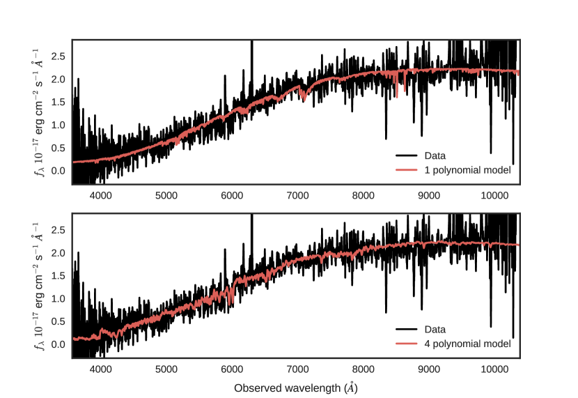
Figure 9.— Example of an object (PLATE 7575 MJD 56947 FIBERID 434) in which a cubic-polynomial model returned a successful measurement while the constant-polynomial measurement failed. The data are shown in black, and the best-fit model is shown in red.

At this point, it is clear that a constant-polynomial term produces lower failure rates, and is empirically the best choice for our data set. Further, a qualitative understanding of the failure modes of the two model types leads us to believe that, in the presence of better flux calibration, the failure rates of a constant-polynomial are likely to decrease further. Thus, we use a constant-polynomial model to classify the eBOSS LRG sample and in all subsequent analyses.

3.2. Determination of $\Delta\chi_{\mathrm{threshold}}^{2}$

Decreasing the value of $\Delta\chi_{\mathrm{threshold}}^{2}$ relaxes the requirement for a declaration of statistical confidence, resulting in higher redshift completeness rates. Doing so comes at the expense of higher rates of catastrophic failures, as incorrect measurements that would have been flagged at a higher threshold are allowed through with no ZWARNING flag. Similarly, increasing the value of $\Delta\chi_{\mathrm{threshold}}^{2}$ decreases catastrophic failure rates as it restricts statistical confidence to only the best of fits, but does so at the expense of completeness rates, reducing usable sample size and statistical power towards cosmology constraints. Thus, determining a value of $\Delta\chi_{\mathrm{threshold}}^{2}$ means striking an optimal balance between completeness and purity while ensuring science requirements are met. Here, we remind the reader that $\Delta\chi_{\mathrm{threshold}}^{2}$ is always scaled to the degrees of freedom to account for possibly varying degrees of freedom between fits, where the number of degrees of freedom is defined as the number of unmasked pixels in the spectrum less the number of template components (i.e., $n_{\mathrm{pix}}-(n_{\mathrm{poly}}+1)$).

We first investigate the failure rate as a function of $\Delta\chi_{\mathrm{threshold}}^{2}$, as shown in Figure 10. At $\Delta\chi_{\mathrm{threshold}}^{2}=0.01$, the value used by spectro1d, redmonster reduces the failure rate from 24.3% to 16.3%. While significant, the failure rate is still more than a factor of 1.5 times the desired $\leq 10$% failure rate for eBOSS science. To ensure sub-10% failure rates, the ZWARNING flag for SMALL_DELTA_CHI2 would need to be set at or below $\Delta\chi_{\mathrm{threshold}}^{2}=0.005$.

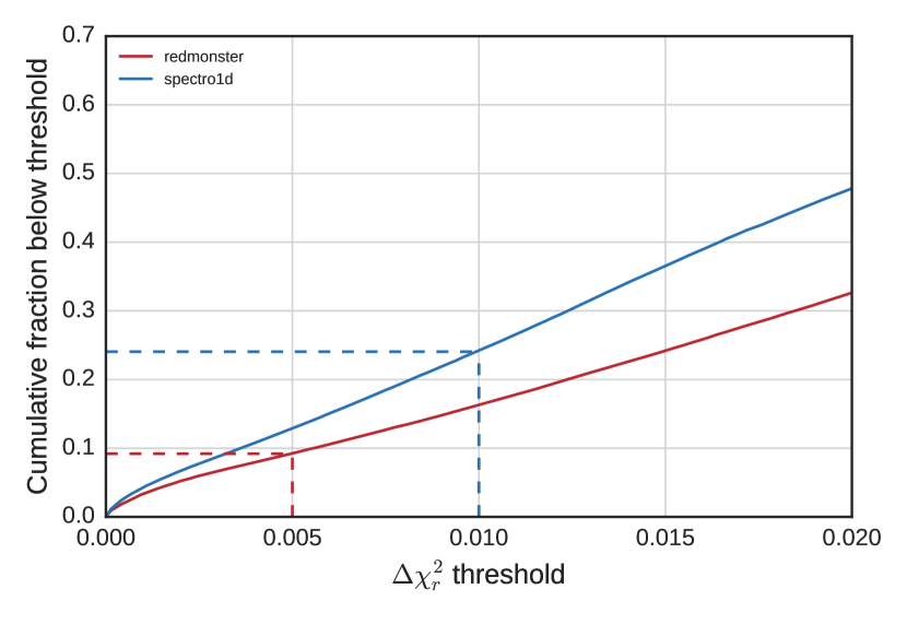
Figure 10.— Redshift failure (ZWARNING $>0$) rate of redmonster and spectro1d pipelines as a function of $\Delta\chi_{\mathrm{r,threshold}}^{2}$to trigger the SMALL_DELTA_CHI2 bit. Dashed red and blue lines serve to visually illustrate the failure rates of redmonster and spectro1d at $\Delta\chi_{\mathrm{r,threshold}}^{2}$ values of 0.005 and 0.01, respectively.

While quantifying completeness is straightforward, doing so for catastrophic failure rates is not. The eBOSS science requirement for catastrophic failures is $<1\%$. By definition, catastrophic failures pass through the software unnoticed, making identification difficult. We consider two tests to characterize the rate of catastrophic failures.

We first asses the completeness of eBOSS sky fibers as a function of $\Delta\chi_{\mathrm{threshold}}^{2}$ as a proxy for catastrophic failures. Sky fibers are those fibers that are not placed on any target, but rather are intended to measure the sky emission, unpolluted by astronomical objects, to aid in sky-subtraction. Roughly $\sim 10\%$ of the fibers on each eBOSS plate are placed as sky fibers. While a small fraction of these will inevitably be placed over real objects, the vast majority should contain no object at all. These should trigger the softwares’ SMALL_DELTA_CHI2 flag since there is no astronomical object; a confident redshift is impossible. While the rate of false positives within this sample is not a direct measurement of the catastrophic failure rate, it does provide a testing ground for the software’s behavior in the limit of low signal-to-noise. As signal-to-noise is the best predictor of redshift measurement success, this sample is informative of the true rates of catastrophic failures. The left panel of Figure 11 shows the cumulative fraction of eBOSS sky fibers above a given $\Delta\chi_{\mathrm{threshold}}^{2}$ for redmonster and spectro1d. At a given threshold, redmonster returns a factor of seven fewer confident measurements.

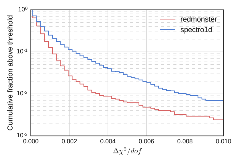
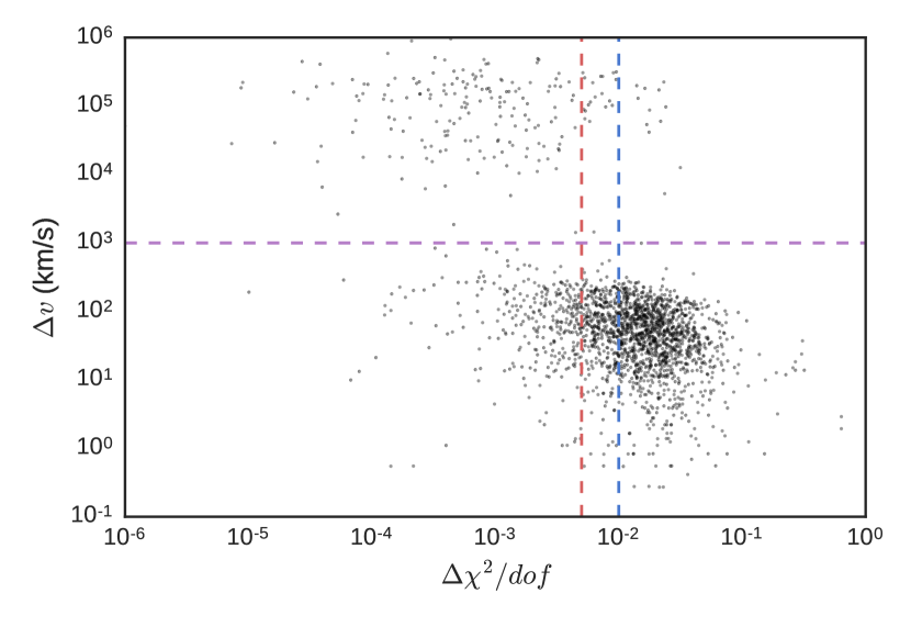
Figure 11.— Left: Cumulative fraction of eBOSS sky fibers with confident redshift measurement and classification as a function of $\Delta\chi_{\mathrm{threshold}}^{2}$. Right: Scatterplot showing redshift difference (in km s^-1) between independent observations of the same LRG target. The red and blue vertical lines represent $\Delta\chi^{2}/\mathrm{dof}$ thresholds of 0.005 and 0.01, respectively. The horizontal dashed line shows the limit of velocity difference to be considered a catastrophic failure.

The increased rigidity of modeling with a single, physically-motivated template over a set of PCA basis vectors reduces the ability of redmonster to fit sky residuals and noise, greatly reducing its rate of false positives. The eBOSS science requirement for catastrophic failures is $<1\%$, which we see in redmonster at a $\Delta\chi_{\mathrm{threshold}}^{2}$ value of $\sim~{}0.004$. In spectro1d, meanwhile, it does not reach sub-1% values until $\sim 0.008$.

We then assess the redshift differences between different spectra of the same object, as in Dawson et al. (2016). First, we identified 2128 targets that were tiled on more than one plate and, thus, have multiple independent observations. We then compared redshift differences as a function of $\Delta\chi^{2}/\mathrm{dof}$, as shown in the right panel of Figure 11. Assuming that, in the cases of discrepant redshifts, one redshift is correct, the rate of catastrophic failures can be estimated by counting objects with $\delta z>1000$ km s^-1 and $\Delta\chi^{2}/\mathrm{dof}$ above the threshold. For this sample, there are 12 catastrophic failures out of 2520 confident measurements for $\Delta\chi_{\mathrm{threshold}}^{2}=0.01$ and 32 catastrophic failures out of 3270 confident measurements for $\Delta\chi_{\mathrm{threshold}}^{2}=0.005$, corresponding to catastrophic failure rates of $0.48\pm 0.14$% and $0.98\pm 0.22$%, respectively. A similar analysis for the spectro1d reductions yields failure rates of $0.35\pm 0.11$% and $0.92\pm 0.16$%.

In order to maximize completeness while maintaining an acceptable catastrophic failure rate, we set $\Delta\chi_{\mathrm{threshold}}^{2}=0.005$ for all subsequent analyses. We also use $\Delta\chi_{\mathrm{threshold}}^{2}=0.01$ for spectro1d when making comparisons, to ensure that the catastrophic failure rate requirement is being met in both sets of reductions. Amongst the full set of eBOSS LRG target spectra, we find an automated completeness (ZWARNING == 0) rate of 90.5%, with a catastrophic failure rate of 0.98%. Meanwhile, spectro1d produces a completeness of 75.6% with a catastrophic failure rate of 0.32%. Thus, redmonster satisfies the requirements of completeness and purity, while spectro1d does not. This improvement is illustrated by the dashed lines in Figure 10.

4. Classification of LRG spectra from eBOSS

We made use of 99,449 eBOSS LRG targets reduced with tagged version v5_10_0 of idlspec2d to demonstrate the performance of redmonster. Galaxy redshift success dependence is described in §4.1, the effect on the final LRG sample redshift distribution is described in §4.2, and galaxy redshift precision and accuracy in §4.3. A description of composite spectra and the distribution of physical galaxy parameters in the sample is given in §4.4.

4.1. Galaxy redshift success dependence

As in all redshift surveys, spectroscopic S/N is the primary determinant of redshift success. In the eBOSS LRG sample, 95.4% of spectra with ZWARNING $>$ 0 are due solely to a SMALL_DELTA_CHI2 failure. Figure 12 shows the dependence of the LRG galaxy redshift failure rate as a function of the median spectroscopic signal-to-noise ratio over the SDSS r, i, and z bandpass ranges. These represent the most relevant regions of the spectrum for measuring redshifts of passive galaxies over the redshift range of interest for the large-scale structure science in eBOSS. Failure is defined in the sense of ZWARNING $>0$, so that targets confidently identified as objects other than galaxies are counted as a success for the pipeline. We see a decrease in the failure rate as a function of r-band S/N up to S/N $\sim 1.8$, where it becomes asymptotic to $\sim 3\%$. The $i$- and $z$-bands behave in a more expected manner, with failure rate decreasing until S/N $\sim 4$, where it reaches an asymptotic minimum of $\sim 2\%$. The $i$- and $z$-band S/N is more predictive of redshift success rate due to the 4000 Å break and the small number of strong narrow absorption features (e.g., Ca H&K, Na I, etc.) being located in those bands over the targeted redshift range.

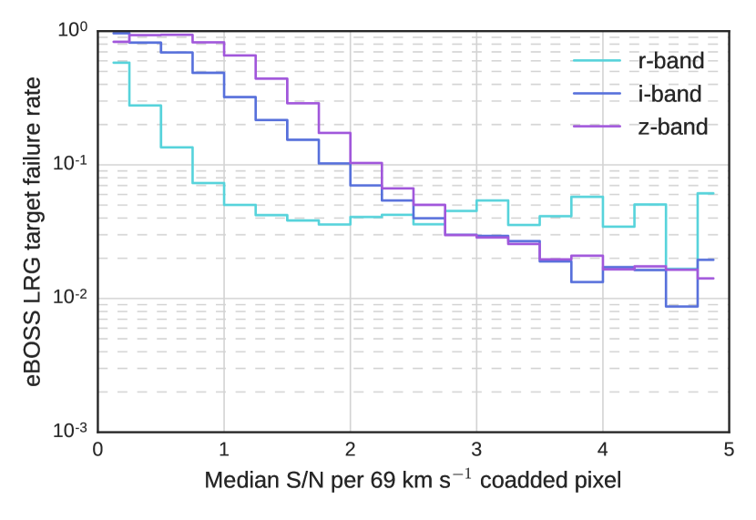
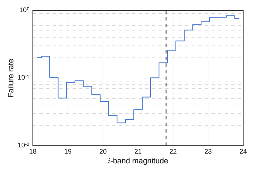
Figure 12.— Left: Redshift failure (ZWARNING $>0$) rate of the eBOSS LRG sample as a function of median S/N in SDSS $r$-, $i$-, and $z$-bands. Right: Redshift failure (ZWARNING $>0$) rate of the eBOSS LRG sample as a function of SDSS $i$-band magnitude. The dashed vertical line indicates the faint-magnitude limit of $i=21.8$.

Galaxy magnitude correlates strongly with spectroscopic S/N and hence with redshift success; this is the motivation for the $i$-band magnitude limit of $<21.8$ in the target selection algorithm. To assess the dependence of redshift completeness on target selection, the right panel of Figure 12 shows the LRG sample’s redshift failure rate as a function of $i_{\mathrm{fiber}}$, defined as the $i$-band magnitude in a 2″ diameter eBOSS fiber. At the formal eBOSS LRG magnitude cutoff, the marginal failure rate is $\sim~{}11\%$.

Additionally, redshift success has a weak dependence on fiber identification number along the spectrograph slit heads. The left panel in Figure 13 shows this effect for eBOSS LRGs. Upturns near fibers 1, 500 and 1000 are due to imperfections in the camera optics near the edge of the spectrograph focal plane. Narrow peaks, such as those around fibers 525-530, are due to bad CCD columns. Fiber numbers below 500 show a higher average failure rate (9.4%) than those above 500 (9.0%) due to lower end-to-end throughput of spectrograph 1 relative to spectrograph 2 (Smee et al., 2013).

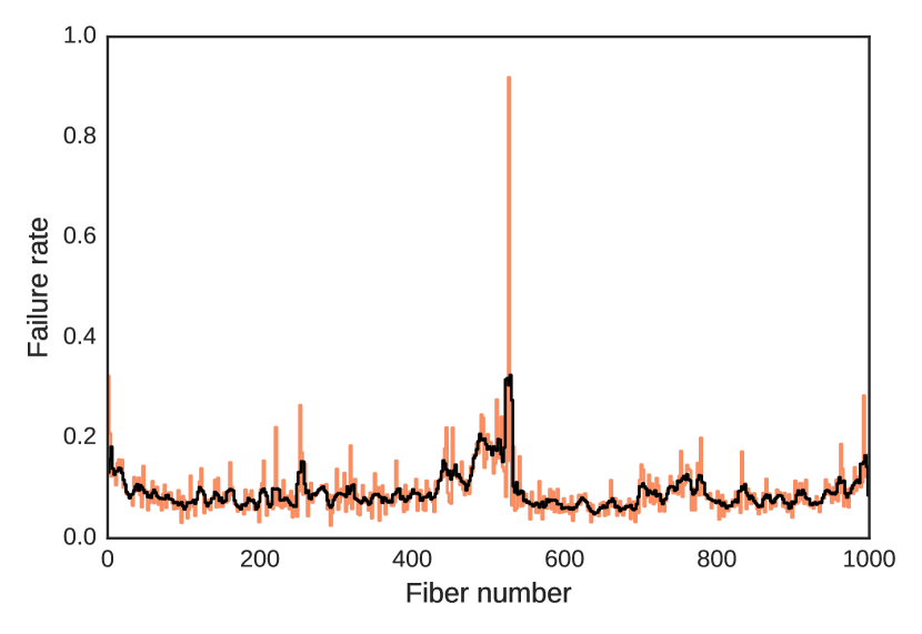
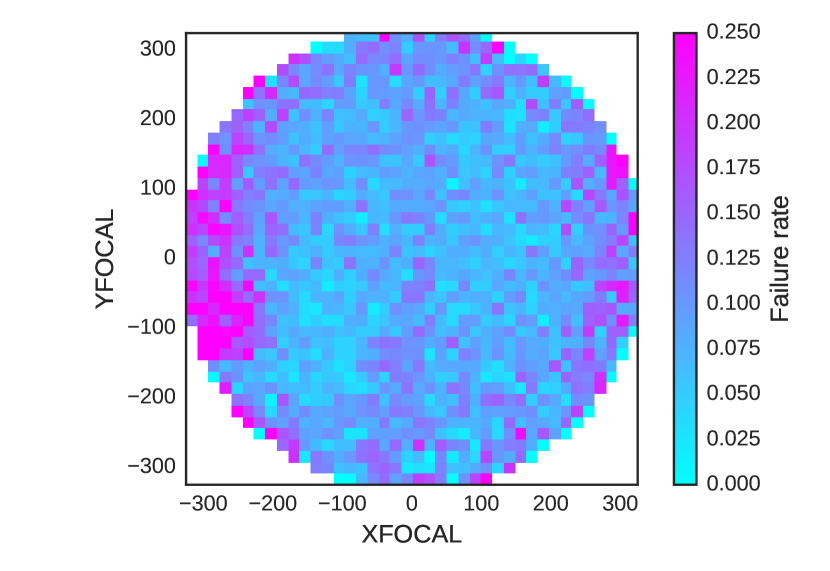
Figure 13.— Left: eBOSS LRG sample failure rate as a function of fiber number. The orange plot shows individual fibers, while the black has been smoothed by 5 pixels to highlight large-scale structure. Right: Failure rate of eBOSS LRG sample as a function of location of fiber head on the physical plug plate.

Finally, we investigated the dependence of failure rate on the location of the fiber on the plug plate. The right panel of Figure 13 shows this relationship. The fibers within the central region covering 50% of the total area show failure rates of $7.8\%$. However, near the edges and, particularly, the left and right sides of the plate, failure rates spike to values of 25% or greater. Plates are generally plugged in a counter-clockwise direction, beginning in the first quadrant, meaning the right edge of the plate contains fibers near 1 and 1000, while the left edge contains fibers near 500; thus, the increased failure rates at the extreme values of XFOCAL are primarily due to the imperfect spectrograph optics described above.

4.2. Effect on final redshift distribution and cosmological projections

In order to quantify the effects of the redmonster spectral classification on the survey’s expected cosmological constraints, we compare the resulting redshift distribution to the predictions presented in Dawson et al. (2016). Those cosmological projections were based on the redshift distribution derived from visually inspected redshifts and classifications for 1997 LRG targets across 16 plates. Plates with deeper than average observations were intentionally chosen to facilitate these visual inspections. These spectra were processed using idlspec2d tagged version v5_8_0, and were visually inspected by ten members of the eBOSS team in August 2015. Each spectrum was manually assigned a redshift and spectral classification, as well as a confidence value $q_{\mathrm{conf}}$ ranging from 0 (entirely uncertain) to 3 (entirely certain). A full qualitative description of all $q_{\mathrm{conf}}$ values is given in Dawson et al. (2016). A subset of plates was inspected by two people, providing a degree of self-calibration of the results.

Table 3 Redshift distribution for the LRG sample from visual inspections, spectro1d, and redmonster using tagged versions v5_9_0 and v5_10_0 of the reductions. The surface densities are presented in units of deg^-2 assuming that 100% of the objects in the parent sample are spectroscopically observed. Entries highlighted in bold font denote the fraction of the sample that satisfies the high-level requirement for the redshift distribution of the sample.

	Visual	Visual	spectro1d	redmonster	spectro1d	redmonster
	($q_{\mathrm{conf}}>0$)	($q_{\mathrm{conf}}>1$)	(DR13)	(DR13)	(DR14)	(DR14)
Poor Spectra	4.0	6.7	17.7	7.7	14.3	5.7
Stellar	5.3	5.3	6.5	2.9	5.4	4.9
$0.0<z<0.5$	0.6	0.6	0.6	0.5	0.6	0.5
$0.5<z<0.6$	6.2	5.9	5.2	6.2	3.4	6.2
$0.6<z<0.7$	15.2	14.8	11.3	14.3	12.4	14.7
$0.7<z<0.8$	15.3	14.7	11.4	16.1	12.9	15.3
$0.8<z<0.9$	9.4	8.7	5.6	8.8	6.8	8.9
$0.9<z<1.0$	3.2	2.7	1.4	2.5	1.7	2.7
$1.0<z<1.1$	0.5	0.4	0.3	0.9	0.3	1.0
$1.1<z<1.2$	0.1	0.1	0.1	0.2	0.1	0.2
Total Targets	60	60	60	60	60	60
Total Tracers	43.1	41.0	29.7	41.7	33.9	41.7

The survey science goals require a minimum of 40 deg^-2 spectroscopically confirmed LRGs in the redshift range $0.6<z<1.0$. To compensate for incomplete fiber assignment, the LRG parent sample is selected at a surface density of 60 deg^-2. Table 3 shows the estimated final tracer density of the LRG sample, binned by redshift. We show the optimistic ($q_{\mathrm{conf}}>0$) and conservative ($q_{\mathrm{conf}}>1$) scenarios from the visual inspections alongside the redmonster and spectro1d N$(z)$ results using reduction versions v5_9_0 and v5_10_0. The surface density of tracers is increased by redmonster relative to spectro1d by 40.4% and 23.9% in DR13 and DR14, respectively. While the improvements to the reductions described in §3 increased the rate of successful redshifts by spectro1d by 14.1%, the tracer density for redmonster remained constant at 41.7 deg^-2. Twenty-six percent of spectra that were previously failures were reclassified by redmonster as stars in the improved reductions. In the optimistic case using extra deep spectra, the visual inspections report a failure of $\sim 6.7$%, while redmonster finds a failure rate of 7.4% on those same spectra. This suggests redmonster is producing failure rates nearly as low as what any software can achieve.

We use the final redshift distribution from redmonster to predict changes to the cosmological projections given in Dawson et al. (2016). Those projections were made using the conservative case ($q_{\mathrm{conf}}>1$) of the visual inspections. The surface density of tracers using redmonster is increased by $3.5\%$ relative to those used in the projections. Because the measurements of cosmological parameters are Poisson-limited, redmonster provides an additional 2% margin on achieving the cosmological precision expected from the eBOSS LRG sample.

4.3. Galaxy redshift precision and accuracy

Redshift errors are calculated from the curvature of the $\chi^{2}(z)$ function in the vicinity of the value that is used to determine the best-fit redshift measurement. To assess the precision of these statistical error estimates, we used the same repeat spectra as those used to assess catastrophic failure rates. We scaled the redshift difference between the two observations by the quadrature sum of the error estimates from the spectra from each observation. We then assessed the full distribution of the velocity differences and fit it with a Gaussian function. If the estimated errors accounted for all the statistical uncertainty, the fit would have a dispersion parameter of unity and a mean of zero. Figure 14 shows the results of this analysis. The fitted dispersion is $\sigma=0.65$ and the mean is $\mu=0.01$. Thus, redshift errors are overestimated by $\sim$54%, meaning that redshift estimates are more precise than reported. A similar analysis performed on the spectro1d reductions of the SDSS-III CMASS (for “constant mass”) galaxy sample ($0.4\lesssim z\lesssim 0.7$) in Bolton et al. (2012) resulted in a fitted dispersion parameter of $\sigma=1.19$.

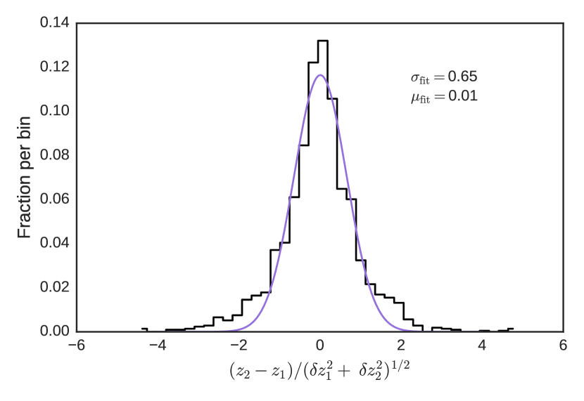
Figure 14.— Histogram of redshift differences of eBOSS LRG targets on extra-deep plates that have had observations split into spectra of typical eBOSS depth, scaled by the quadrature sum of the statistical error estimates of each split. Over-plotted is the best-fit Gaussian model, with a standard deviation of $\sigma=0.65$ and a mean of $\mu=0.01$.

Next, we examine the statistical redshift error distributions as a function of median S/N in the SDSS $r$-, $i$-, and $z$-bands, and find a weak anti-correlation. This is as expected, and is consistent with previous SDSS data sets. A summary of these statistics is given in Table 4. Finally, for all LRG targets, we also compute the distribution of estimated redshift errors as a function of redshift. A summary of the statistics is given in Table 5. In all cases, typical errors are a few tens of km s^-1. They should be reduced by an additional factor of 1.54 to reflect the statistical scatter displayed in Figure 14. These errors are well below the 300 km s^-1 redshift precision requirement of the eBOSS galaxy large-scale structure and redshift space distortion science analyses.

Table 4 Mean and standard deviation of estimated statistical redshift error in several S/N bins in SDSS $r$-, $i$-, and $z$-bands. Values are given in km s^-1.

SDSS band	S/N range	$\bar{\sigma}_{\mathrm{v}}$	Var$(\sigma_{\mathrm{v}})^{1/2}$
$r$	$1.0<$ S/N $<1.5$	34.50	10.41
$r$	$1.5<$ S/N $<2.0$	28.10	8.83
$r$	$2.0<$ S/N $<2.5$	22.38	7.99
$r$	$2.5<$ S/N $<3.0$	18.59	15.25
$i$	$1.0<$ S/N $<1.5$	52.18	17.40
$i$	$1.5<$ S/N $<2.0$	46.50	14.80
$i$	$2.0<$ S/N $<2.5$	41.56	12.52
$i$	$2.5<$ S/N $<3.0$	36.76	9.97
$i$	$3.0<$ S/N $<3.5$	32.89	8.88
$i$	$3.5<$ S/N $<4.0$	29.56	8.48
$z$	$1.0<$ S/N $<1.5$	51.51	16.88
$z$	$1.5<$ S/N $<2.0$	46.10	13.99
$z$	$2.0<$ S/N $<2.5$	40.38	10.96
$z$	$2.5<$ S/N $<3.0$	35.68	9.42
$z$	$3.0<$ S/N $<3.5$	32.02	8.49
$z$	$3.5<$ S/N $<4.0$	28.93	7.38

Table 5 Mean and standard deviation of estimated statistical redshift error in several redshift bins. Values are given in km s^-1.

Redshift range	$\bar{\sigma}_{\mathrm{v}}$	Var$(\sigma_{\mathrm{v}})^{1/2}$
$0.6<z<0.7$	37.36	12.24
$0.7<z<0.8$	38.69	13.21
$0.8<z<0.9$	41.70	15.23
$0.9<z<1.0$	45.22	17.33

4.4. Composite spectra and distribution of galaxy parameters

A primary advantage of redmonster over PCA-based redshift classification techniques is the simple manner in which the best-fitting template can be translated to physical parameters. In this section, we briefly discuss two types of analyses made possible by this parameterization. We seek only to demonstrate these possibilities and defer analysis of the results to a later work.

Stacking large numbers of spectra has become a widely-used technique in extragalactic physics and cosmology. We derive composite spectra of high signal-to-noise ratios to enable analysis of the quality of our templates in relation to the true spectral features in eBOSS galaxies. Previous work (e.g., Eisenstein et al., 2003) concentrated on analyzing and averaging spectra based on observed quantities, such as color or magnitude. The physicality of the redmonster parameterization allows us to separate and bin our galaxy sample based on quantities such as age, velocity dispersion, emission line ratio and strength, metallicity, and star formation history (SFH), as determined by the best-fitting template.

We first binned a subset of the eBOSS galaxy sample based on the age of the template that produced the best-fit model. Objects were chosen with best-fitting templates of zero line flux to identify a passively-evolving sample. To derive meaningful composites, these spectra then must be normalized. Due to the relatively low signal-to-noise of eBOSS spectra, we cropped the noisy blue- and red-end of each spectrum, and scaled the spectrum such that the median of the pixels in the wavelength range $4000<\lambda<9000$ is unity. We scaled the template corresponding to each bin to fit the composite spectrum. Example composite spectra for observed spectra best fit by the 0.56 Gyr, 1.0 Gyr, 1.78 Gyr, 3.16 Gyr, and 5.62 Gyr templates are shown in Figure 15; they contain 412, 1,486, 14,739, 22,288, and 11,134 unique galaxies, respectively. We stress that these composites are selected only by template age; metallicity is assumed to be solar (Asplund et al., 2009) and velocity dispersion is assumed to be 250 km s^-1. An example of fitting similar composites over the wavelength range $0.4-0.8\mu m$ while allowing metallicity and velocity dispersion to vary is given in Conroy et al. (2014). These eBOSS data will allow a similar analysis to be extended to shorter wavelengths.

In general, the templates better describe the continuum in the red than the blue. The templates systematically over-estimate flux density between $\sim 2500$ Å and $\sim 3600$ Å. All three templates have a broad feature at $\sim 2700$ Å that is exaggerated relative to the composite spectra, likely due to missing atomic opacities in the models. Discrepancies in the continuum may be due to the effects of dust attenuation. In the core fitting algorithm, these effects can be accounted for by the polynomial nuisance vectors; the models in this figure are scaled to the composite spectra without any polynomial terms, allowing the effects of dust in the data to appear as shortcomings in the templates. On the other hand, the models are able to reproduce the observed behavior of the narrow-band features. All five composite spectra clearly display lines from the Mg II doublet (2796 Å and 2803 Å), Ca H&K (3934 Å and 3968 Å), H$\delta$ (4103 Å), G-band (4307 Å), and H$\beta$ (4863 Å) that are well fit by the templates. The 0.56 Gyr and 1.0 Gyr composite spectra have a well-fit H$\gamma$ line (4341 Å) and more prominent Balmer features, as expected from a younger stellar population. Additionally, an Mg I line at 2852 Å, a band of Mg I absorption just blueward of Ca H&K, and an Mg I line at 5175 Å become more prominent at older stellar populations.

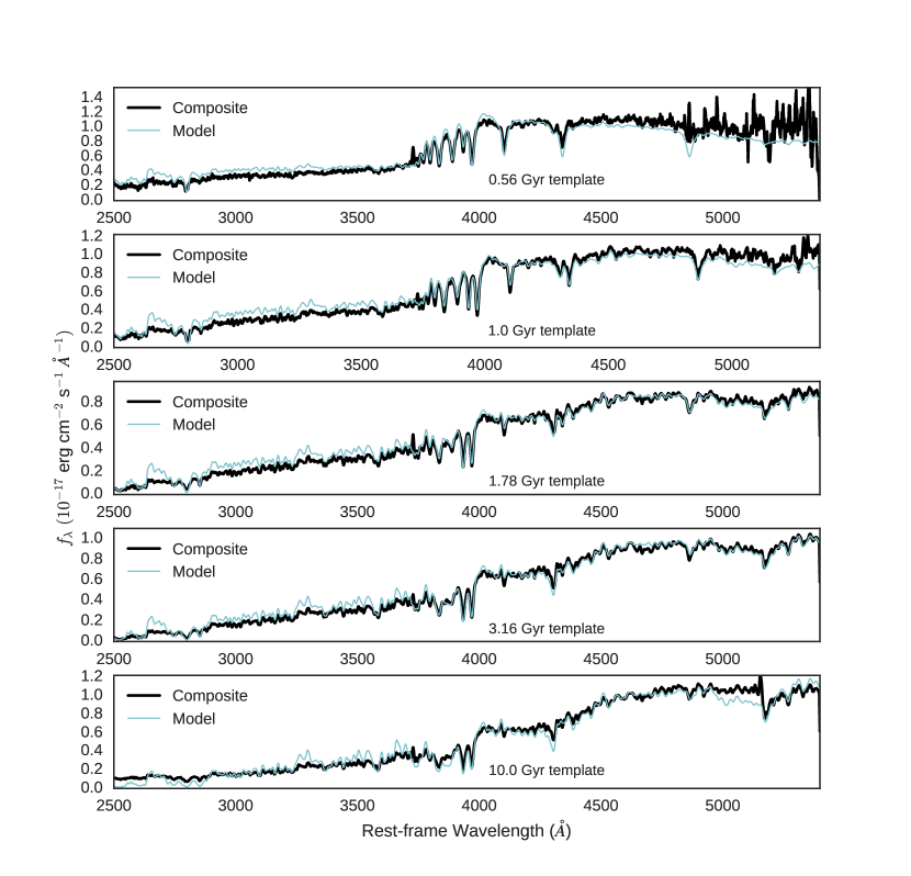
Figure 15.— Composite spectra for five ages as estimated by redmonster. The data are shown in black, and the template of corresponding age is shown in teal. Here, age is the only free parameter; thus, one should not over-interpret mismatches between composites and models.

Next, we evaluate the distribution of the physical parameters across the galaxy sample. These distribitions are informative of both the accuracy of the spectral features in the templates and the targeting completeness and selection bias of the survey. As an example, we again consider galaxy template age. We binned our sample into four redshift bins and show the distribution of the ages of the best-fit templates in Figure 16. The mean values of the four redshift bins, $0.5<z<0.6$, $0.6<z<0.7$, $0.7<z<0.8$, and $0.8<z<0.9$, are 4.9 Gyr, 4.3 Gyr, 3.9 Gyr, and 3.7 Gyr, respectively. Assuming a $\Lambda$CDM cosmology with $k=0$, $H_{0}=67.8$ km s^-1 Mpc^-1, $\Omega_{\mathrm{m}}=0.308$, and $w_{\Lambda}=-1$ (Planck Collaboration et al., 2015), the age of the universe at redshifts $z=0.56$, $z=0.65$, $z=0.75$, and $z=0.84$, the sample mean in each bin, is 8.18 Gyr, 7.61 Gyr, 7.03 Gyr, and 6.57 Gyr, respectively. A comparison with the median template age in each bin reveals a galaxy sample that ages more slowly than the universe. Due to not allowing metallicity and abundance patterns to be fit as free parameters (as the templates in this paper use only solar metallicity), it is likely not possible to meaningfully interpret the ages. However, a more careful analysis could be used to investigate targeting selection bias in the survey.

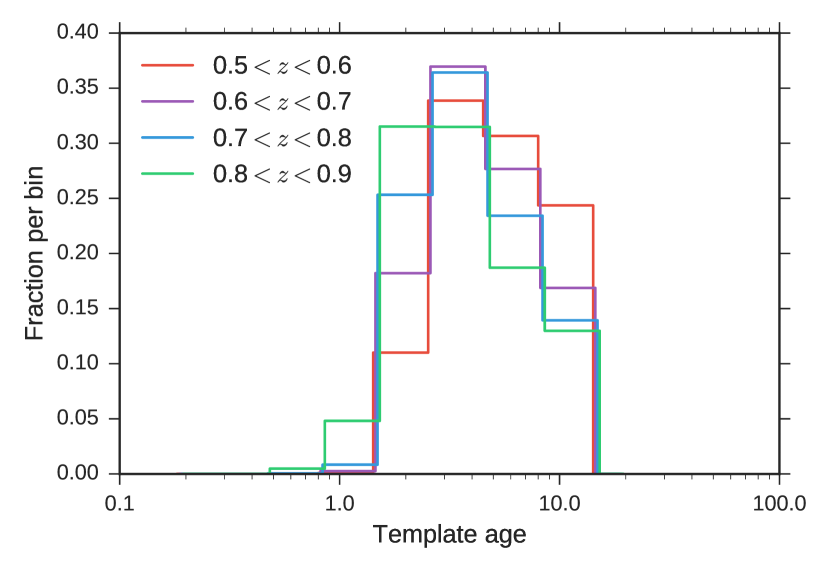
Figure 16.— Distributions of the age of the template component in the best-fit model to each spectrum in four redshift slices.

5. Summary and Conclusion

We have described the redmonster software that provides automated redshift measurement and spectral classification and its performance on the SDSS-IV eBOSS LRG sample, comprising 99,449 spectra. This software provides a new algorithm and new sets of templates that restrict all spectral fitting to only physically-motivated models. The advantages over the current algorithm include robustness against unphysical solutions likely to arise for low signal-to-noise spectra (particularly in the presence of imperfect sky-subtraction), determination of joint likelihood functions over redshift and physical parameters, and custom configurability of spectroscopic templates for different target classes.

The redshift success rate of the redmonster software on eBOSS LRGs is 90.5%, meeting the eBOSS scientific requirement of 90% and providing a significant improvement over the previous redshift pipeline, spectro1d. The improvement translates to a 23.9% increase in the surface density of tracers that can now be used to constrain cosmology through clustering measurements. We have shown catastrophic failure rates for redmonster of 0.98%, in agreement with the scientific requirements of $<1$%. The software also provides robust estimates of statistical redshift errors that are Gaussian distributed, typically a few tens of km s^-1, well below the specified maximum of 300 km s^-1.

Looking forward, using $\Delta\chi_{\mathrm{threshold}}^{2}=0.0015$ would give redmonster a completeness of 95.7% and a catastrophic failure rate of 1.9%, which would very nearly meet the DESI science requirements of at least 95% completeness and a maximum of 5% catastrophic failures on eBOSS data. The raw S/N in DESI will be comparable to that in eBOSS, though the image quality in eBOSS two-dimensional spectra is degraded relative to the image quality we expect in the bench-mounted DESI system. eBOSS also shows a failure rate that increases to $\sim 25\%$ near the edges of the focal plane. This is imperfect optics towards the edges of the spectrographs, which will be less significant in DESI. Therefore, we expect improved redmonster performance on the more well-behaved DESI spectra.

Development work is ongoing for eBOSS, both in the calibration and extraction of spectra and on redmonster itself. The next priority for redmonster development is to build and test templates for ELG and quasar spectra. Additionally, we will incorporate simultaneous fitting to the individual exposures at their native resolution to remove covariances between neighboring pixels introduced by the co-adding process. Subsequent eBOSS data releases will be accompanied by catalogues of redshift measurements and spectral classifications produced by redmonster.

Appendix A Output files

The redmonster software generates two output files for each input set of spectra and summary files of all objects processed by the software. The “redmonsterAll” file is the primary output and contains all redshifts, spectral classifications, parameter estimates, and models, and is described in §A.0.1. The “chi2arr” file is an optional output containing the entire $\chi^{2}(\vec{P},z)$ surface for a template class and is described in §A.0.2. A more detailed description of these files can be found in the online documentation.

A.0.1 redmonster files

The “redmonsterAll” file is the primary output of the software. This file contains all redshift and parameter measurements, spectral classifications, and the best fit model for each object. This output is an uncompressed FITS file with all relevant information in the primary HDU header and first BIN table. The contents of the BIN table are detailed in Table 6. It has the naming scheme redmonsterAll-vvvvvv.fits, where vvvvvv is the version of the reduction used. This file is the parallel to the spAll file produced by spectro1d in BOSS and eBOSS.

Additionally, a batch file is created for each batch of spectra processed. It is the parallel to spectro1d’s spZall for an SDSS plate in BOSS and eBOSS, and is named redmonster-pppp-mmmmm.fits, where pppp is the plate number and mmmmm is the MJD. The file contains a primary header, a binary extension (similar in format to that of redmonsterAll) containing the best five redshifts and classifications for each fiber, and an imageHDU containing a two-dimensional image of the five best-fit models for all fibers. The size of this file is approximately 20 MB for 1000 spectra of $\sim 4600$ pixels each.

A.0.2 chi2arr file

The software also has the ability to write the full $\chi^{2}(\vec{P},z)$ surfaces for each template class to an output file. These are also uncompressed FITS files. The primary HDU contains a multi-dimensional image of all $\chi^{2}$ values for a single template class for each spectrum. These files follow the naming scheme chi2arr-ttttttt-vvvvvv.fits, where tttttt is the name of the template class and vvvvvv is the version of the reduction used. The primary HDU contains a multi-dimensional array of the full $\chi^{2}$ surface for that template class. These files are written per batch of spectra processed. A summary file similar to redmonsterAll does not exist due to the large size of these files (often several GB per 1000 spectra).

Table 6 redmonsterAll file binary table contents

Name	Description
FIBERID	spPlate fiber number (0-based) for each object
PLATE	spPlate plate number for each object
MJD	spPlate MJD for each object
DOF	Degrees of freedom used to calculate $\chi_{\mathrm{red}}^{2}$
BOSS_TARGET1	BOSS targeting bit
EBOSS_TARGET0	SEQUELS targeting bit
EBOSS_TARGET1	EBOSS targeting bit
Z	Best redshift (least $\chi_{\mathrm{red}}^{2}$)
Z_ERR	1-$\sigma$ error associated with Z
CLASS	Object type classification
SUBCLASS	Best-fit template parameters
FNAME	Full name of ndArch file of template
MINVECTOR	Coordinates of best-fit template in ndArch file
MINRCHI2	$\chi_{\mathrm{red}}^{2}$ value of fit
NPOLY	Number of additive polynomials used
NPIXSTEP	Pixel step size used
THETA	Coefficients of template and polynomial terms in fit
ZWARNING	ZWARNING flags
RCHI2DIFF	$\Delta\chi_{\mathrm{red}}^{2}$ between first- and second-best fits
CHI2NULL	$\chi_{\mathrm{null}}^{2}$ value for each spectrum
SN2DATA	(S/N)2 of each spectrum

Note. — Each SDSS plate’s reduction file contains the best five redshifts, errors, and classifications (Z1, Z_ERR1, CLASS1, etc.).

References

- Alam et al. (2015) Alam, S., Albareti, F. D., Allende Prieto, C., et al. 2015, ApJS, 219, 12
- Allende Prieto et al. (2003) Allende Prieto, C., Lambert, D. L., Hubeny, I., & Lanz, T. 2003, ApJS, 147, 363
- Allende Prieto (2008) Allende Prieto, C. 2008, Physica Scripta Volume T, 133, 014014
- Asplund et al. (2005) Asplund, M., Grevesse, N., & Sauval, A. J. 2005, Cosmic Abundances as Records of Stellar Evolution and Nucleosynthesis, 336, 25
- Asplund et al. (2009) Asplund, M., Grevesse, N., Sauval, A. J., & Scott, P. 2009, ARA&A, 47, 481
- Barklem et al. (2000) Barklem, P. S., Piskunov, N., & O’Mara, B. J. 2000, A&AS, 142, 467
- Barklem & Piskunov (2015) Barklem, P. S., & Piskunov, N. 2015, Astrophysics Source Code Library, ascl:1507.008
- Beutler et al. (2011) Beutler, F., Blake, C., Colless, M., et al. 2011, MNRAS, 416, 3017
- Blanton et al. (2016) Blanton, et al. 2016, in preparation
- Bolton et al. (2012) Bolton, A. S., Schlegel, D. J., Aubourg, É., et al. 2012, AJ, 144, 144
- Chen et al. (2012) Chen, Y.-M., Kauffmann, G., Tremonti, C. A., et al. 2012, MNRAS, 421, 314
- Cole et al. (2005) Cole, S., Percival, W. J., Peacock, J. A., et al. 2005, MNRAS, 362, 505
- Comparat et al. (2015) Comparat, J., Delubac, T., Jouvel, S., et al. 2015, arXiv:1509.05045
- Conroy et al. (2009) Conroy, C., Gunn, J. E., & White, M. 2009, ApJ, 699, 486
- Conroy & Gunn (2010) Conroy, C., & Gunn, J. E. 2010, ApJ, 712, 833
- Conroy & van Dokkum (2012a) Conroy, C., & van Dokkum, P. 2012, ApJ, 747, 69
- Conroy et al. (2014) Conroy, C., Graves, G. J., & van Dokkum, P. G. 2014, ApJ, 780, 33
- Conroy, Kurucz, Cargile, Castelli, (in prep.) Conroy, C., Kurucz, R., Cargile, P. A., Castelli, F. 2016, in preparation
- Davis et al. (1982) Davis, M., Huchra, J., Latham, D. W., & Tonry, J. 1982, ApJ, 253, 423
- Dawson et al. (2013) Dawson, K. S., Schlegel, D. J., Ahn, C. P., et al. 2013, AJ, 145, 10
- Dawson et al. (2016) Dawson, K. S., et al. 2016, in preparation
- Delubac et al. (2016) Delubac, T., et al. 2016, in preparation
- Eisenstein et al. (2003) Eisenstein, D. J., Hogg, D. W., Fukugita, M., et al. 2003, ApJ, 585, 694
- Eisenstein et al. (2005) Eisenstein, D. J., Zehavi, I., Hogg, D. W., et al. 2005, ApJ, 633, 560
- Eisenstein et al. (2011) Eisenstein, D. J., Weinberg, D. H., Agol, E., et al. 2011, AJ, 142, 72
- Fukugita et al. (1996) Fukugita, M., Ichikawa, T., Gunn, J. E., et al. 1996, AJ, 111, 1748
- Garilli et al. (2014) Garilli, B., Guzzo, L., Scodeggio, M., et al. 2014, A&A, 562, A23
- Glazebrook et al. (1998) Glazebrook, K., Offer, A. R., & Deeley, K. 1998, ApJ, 492, 98
- Gunn et al. (1998) Gunn, J. E., Carr, M., Rockosi, C., et al. 1998, AJ, 116, 3040
- Gunn et al. (2006) Gunn, J. E., Siegmund, W. A., Mannery, E. J., et al. 2006, AJ, 131, 2332
- Harris et al. (2016) Harris, D. W., Jensen, T. W., Suzuki, N., et al. 2016, arXiv:1603.08626
- Heavens (1993) Heavens, A. F. 1993, MNRAS, 263, 735
- Jensen et al. (2016) Jensen, T., Vivek, M., Dawson, K. S., et al. 2016, in preparation
- Jones et al. (2004) Jones, D. H., Saunders, W., Colless, M., et al. 2004, MNRAS, 355, 747
- Kaiser (1987) Kaiser, N. 1987, MNRAS, 227, 1
- Koesterke (2009) Koesterke, L. 2009, American Institute of Physics Conference Series, 1171, 73
- Kroupa (2001) Kroupa, P. 2001, MNRAS, 322, 231
- Kurucz (1970) Kurucz, R. L. 1970, SAO Special Report, 309, 309
- Kurucz & Avrett (1981) Kurucz, R. L., & Avrett, E. H. 1981, SAO Special Report, 391, 391
- Kurucz (1993) Kurucz, R. L. 1993, Kurucz CD-ROM, Cambridge, MA: Smithsonian Astrophysical Observatory, —c1993, December 4, 1993,
- Levi et al. (2013) Levi, M., Bebek, C., Beers, T., et al. 2013, arXiv:1308.847
- Liske et al. (2015) Liske, J., Baldry, I. K., Driver, S. P., et al. 2015, MNRAS, 452, 2087
- Margala et al. (2015) Margala, D., Kirkby, D., Dawson, K., et al. 2015, arXiv:1506.04790
- Marigo et al. (2008) Marigo, P., Girardi, L., Bressan, A., et al. 2008, A&A, 482, 883
- Mészáros et al. (2012) Mészáros, S., Allende Prieto, C., Edvardsson, B., et al. 2012, AJ, 144, 120
- Myers et al. (2015) Myers, A. D., Palanque-Delabrouille, N., Prakash, A., et al. 2015, arXiv:1508.04472
- Newman et al. (2013) Newman, J. A., Cooper, M. C., Davis, M., et al. 2013, ApJS, 208, 5
- Pâris et al. (2012) Pâris, I., Petitjean, P., Aubourg, É., et al. 2012, A&A, 548, A66
- Planck Collaboration et al. (2015) Planck Collaboration, Ade, P. A. R., Aghanim, N., et al. 2015, arXiv:1509.06555
- Prakash et al. (2015) Prakash, A., Licquia, T. C., Newman, J. A., et al. 2015, arXiv:1508.04478
- Raichoor et al. (2016) Raichoor, A., Comparat, J., Delubac, T., et al. 2016, A&A, 585, A50
- Schlegel et al. (1998) Schlegel, D. J., Finkbeiner, D. P., & Davis, M. 1998, ApJ, 500, 525
- Smee et al. (2013) Smee, S. A., Gunn, J. E., Uomoto, A., et al. 2013, AJ, 146, 32
- Tonry & Davis (1979) Tonry, J., & Davis, M. 1979, AJ, 84, 1511
- Wright et al. (2010) Wright, E. L., Eisenhardt, P. R. M., Mainzer, A. K., et al. 2010, AJ, 140, 1868
- York et al. (2000) York, D. G., Adelman, J., Anderson, J. E., Jr., et al. 2000, AJ, 120, 1579