Study of baryon acoustic oscillations with SDSS DR12 data and measurement of $\Omega_{\textrm{DE}}(a)$

Abstract

We define Baryon Acoustic Oscillation (BAO) distances $\hat{d}_{\alpha}(z,z_{c})$, $\hat{d}_{z}(z,z_{c})$, and $\hat{d}_{/}(z,z_{c})$ that do not depend on cosmological parameters. These BAO distances are measured as a function of redshift $z$ with the Sloan Digital Sky Survey (SDSS) data release DR12. From these BAO distances alone, or together with the correlation angle $\theta_{\textrm{MC}}$ of the Cosmic Microwave Background (CMB), we constrain the cosmological parameters in several scenarios. We find $4.3\sigma$ tension between the BAO plus $\theta_{\textrm{MC}}$ data and a cosmology with flat space and constant dark energy density $\Omega_{\textrm{DE}}(a)$. Releasing one and/or the other of these constraints obtains agreement with the data. We measure $\Omega_{\textrm{DE}}(a)$ as a function of $a$.

I Introduction

A point-like peak in the primordial density of the universe results, well after recombination and decoupling, in two spherical shells of overdensity: one of radius $\approx 150$ Mpc, and one of radius $\approx 18$ Mpc Eisenstein ; BAO1 ; BAO2 . (All distances in this article are “co-moving”, i.e. are referred to the present time $t_{0}$.) The “acoustic length scale” $r^{\prime}_{S}\approx 150$ Mpc is approximately the distance that sound waves of the tightly coupled plasma of photons, electrons, protons, and helium nuclei traveled from the time of the Big Bang until the electrons recombined with the protons and helium nuclei to form neutral atoms, and the photons decoupled. The inner spherical shell of $\approx 18$ Mpc becomes re-processed by the hierarchical formation of galaxies BH , while the radius of the outer shell is unprocessed to better than 1% BAO2 (or even 0.1% with corrections BAO2 ) and therefore is an excellent standard ruler to measure the expansion of the universe as a function of redshift $z$. Histograms of galaxy-galaxy distances show an excess of galaxy pairs with distances in the approximate range $150-18$ to $150+18$ Mpc. This “Baryon Acoustic Oscillation” (BAO) signal has a signal-to-background ratio of the order of 0.1% to 1%. Measurements of these BAO signals are by now well established (see BAO1 ; BAO2 for extensive lists of early publications).

In this article we present studies of BAO with Sloan Digital Sky Survey (SDSS) data release DR12 DR12 .

II The homogeneous universe

To establish the notation, let us recall the equations that describe the metric and evolution of a homogeneous universe in the General Theory of Relativity: PDG

$$ds^{2} = dt^{2}-R^{2}(t)\left[\frac{dr^{2}}{1-kr^{2}}+r^{2}(d\theta^{2}+\sin^{2}{\theta}d\phi^{2})\right],$$

$$\frac{H}{H_{0}} \equiv E(a)=\sqrt{\frac{\Omega_{\textrm{m}}}{a^{3}}+\frac{\Omega_{\textrm{r}}}{a^{4}}+\Omega_{\textrm{DE}}(a)+\frac{\Omega_{k}}{a^{2}}},$$ (2)

where the expansion and Hubble parameters are defined as

$$a(t)\equiv\frac{R(t)}{R(t_{0})},\qquad H(t)\equiv\frac{da/dt}{a}.$$ (3)

We rescale $r$ such that the curvature constant $k$ adopts one of three values: $k=0,1$ or $-1$ for a spatially flat, closed or open universe, respectively. Today $t=t_{0}$, $a(t_{0})\equiv a_{0}\equiv 1$ and $H(t_{0})\equiv H_{0}$. The “red shift” $z$ is related to the expansion parameter:

$$a=\frac{1}{1+z}\equiv\frac{f_{0}}{f}$$ (4)

where $f$ and $f_{0}$ are the frequencies of emission and reception of a ray of light as measured by comoving observers. Note that along a light ray $fa$ is constant. $\Omega_{\textrm{m}}/a^{3}$ and $\Omega_{\textrm{r}}/a^{4}$ are, respectively, the densities of non-relativistic matter and ultra-relativistic radiation measured in units of the “critical density” $\rho_{c}\equiv 3H^{2}_{0}/(8\pi G_{N})$. $\Omega_{k}\equiv-k/\left[R(t_{0})H_{0}\right]^{2}$. In the General Theory of Relativity $\Omega_{\textrm{DE}}=\Lambda/(3H_{0}^{2})$, where $\Lambda$ is the “cosmological constant”. To test the theory we let $\Omega_{\textrm{DE}}(a)\equiv\Omega_{\textrm{DE}}f(a)$ (with $f(1)=1$) be a function of $a$ to be determined by observations. Note that from Eq. (2) at $t_{0}$ we obtain the identity

$$\Omega_{\textrm{m}}+\Omega_{\textrm{r}}+\Omega_{\textrm{DE}}+\Omega_{k}\equiv 1.$$ (5)

It is observed that $\Omega_{k}\ll 1$ PDG so we expand expressions up to first order in $\Omega_{k}$. At the late times of interest the density of radiation is negligible with respect to the density of matter so we set $\Omega_{\textrm{r}}=0$.

We consider four scenarios:

1. The observed acceleration of the expansion of the universe is due to the cosmological constant, i.e. $f(a)=1$.

2. The observed acceleration of the expansion of the universe is due to a gas of negative pressure with an equation of state $w\equiv p/\rho<0$. We allow the index $w$ to be a function of $a$ BAO1 ; Linder : $w(a)=w_{0}+w_{a}(1-a)$. While this gas dominates $E(a)$ the equation PDG

   $$\frac{d\rho}{dt}=-3\frac{da/dt}{a}(\rho+p)$$ (6)

   can be integrated with the result BAO1 ; Linder

   $$f(a)=a^{-3(1+w_{0}+w_{a})}\exp{\left\{-3w_{a}(1-a)\right\}}.$$ (7)

   If $w_{0}=-1$ and $w_{a}=0$ we obtain $f(a)=1$ as in the General Theory of Relativity.

3. Same as Scenario 2 with $w(a)$ constant, i.e. $w_{a}=0$.

4. We measure the dependence of $\Omega_{\textrm{DE}}(a)$ on $a$ in the linear approximation

   $$f(a)=1+w_{1}(1-a).$$ (8)

Note that BAO measurements can constrain $\Omega_{\textrm{DE}}(a)$ for $0.5\lesssim a\leq 1$ where $\Omega_{\textrm{DE}}(a)$ contributes significantly to $E(a)$.

III BAO observables

Problem: An astronomer observes two galaxies at the same redshift $z$ separated by an angle $\alpha\lesssim 1$. What is the distance $d^{\prime}_{\alpha}$ between these two galaxies today? Answer to sufficient accuracy:

$$d^{\prime}_{\alpha} \equiv \frac{c}{H_{0}}d_{\alpha}=\frac{c}{H_{0}}2d_{A}(z)\sin{\left(\frac{\alpha}{2}\right)},$$

$$d_{A}(z) = \chi(z)\left(1+\frac{1}{6}\Omega_{k}\chi^{2}(z)\right),$$

$$\chi(z) \equiv \int_{0}^{z}{\frac{dz^{\prime}}{E(z^{\prime})}}.$$ (9)

Here we have written the speed of light $c$ explicitly. The function $\chi(z)$ is presented in Table 1 for some bench mark universes. ($\chi(z)$ is not to be confused with the $\chi^{2}$ of fits.)

Table 1: Function $\chi(z)$ for several values of $z$, $\Omega_{\textrm{m}}$ and $\Omega_{\textrm{DE}}$. $\Omega_{k}=1-\Omega_{\textrm{m}}-\Omega_{\textrm{DE}}$. Measurements at the “Lyman alpha forest” correspond to $z\approx 2.4$. Decoupling of photons occurs at $z=1090.2\pm 0.7$ PDG . All columns have $w_{0}=-1$, $w_{a}=0$, except the row (*) which has $w_{0}=-0.9$, $w_{a}=0$. An approximation to $\chi(z)$ good to an accuracy of $\pm 1\%$ for $z$ in the range 0 to 1 is $\chi(z)=z\exp(-z/z_{c})$ with $z_{c}$ given in the next-to-last row. $r_{S}$ is calculated from Eq. (19) with $\theta_{\textrm{MC}}$ given by (12).

$\Omega_{\textrm{m}}$	0.25	0.30	0.35	0.25	0.30 (*)
$\Omega_{\textrm{DE}}$	0.75	0.70	0.65	0.70	0.70
$\Omega_{k}$	0.00	0.00	0.00	0.05	0.00
$z=0.2$	0.192	0.191	0.189	0.191	0.189
$z=0.4$	0.368	0.362	0.357	0.364	0.357
$z=0.6$	0.526	0.515	0.505	0.520	0.506
$z=0.8$	0.668	0.651	0.635	0.659	0.638
$z=1.0$	0.796	0.771	0.750	0.783	0.756
$z=2.4$	1.400	1.333	1.276	1.371	1.306
$z=3.0$	1.564	1.484	1.417	1.532	1.456
$z=1090.2$	3.416	3.178	2.988	3.368	3.147
$z_{c}$	4.33	3.84	3.48	4.07	3.58
$r_{S}\times 100$	3.557	3.309	3.112	3.839	3.277

Table 2: Function $1/E(z)$ for several values of $z$, $\Omega_{\textrm{m}}$ and $\Omega_{\textrm{DE}}$. $\Omega_{k}=1-\Omega_{\textrm{m}}-\Omega_{\textrm{DE}}$. All columns have $w_{0}=-1$, $w_{a}=0$, except the row (*) which has $w_{0}=-0.9$, $w_{a}=0$. An approximation to $1/E(z)$ good to an accuracy of $\pm 1\%$ for $z$ in the range 0 to 1 is $1/E(z)=(1-z/z_{c})\exp(-z/z_{c})$ with $z_{c}$ given in the last row.

$\Omega_{\textrm{m}}$	0.25	0.30	0.35	0.25	0.30 (*)
$\Omega_{\textrm{DE}}$	0.75	0.70	0.65	0.70	0.70
$\Omega_{k}$	0.00	0.00	0.00	0.05	0.00
$z=0.2$	0.920	0.906	0.893	0.911	0.892
$z=0.4$	0.834	0.810	0.788	0.821	0.791
$z=0.6$	0.751	0.720	0.693	0.735	0.701
$z=0.8$	0.673	0.639	0.610	0.657	0.622
$z=1.0$	0.603	0.568	0.538	0.587	0.554
$z_{c}$	4.33	3.84	3.48	4.07	3.58

Problem: An astronomer observes two galaxies at redshifts $z_{1}$ and $z_{2}$ with a negligible angle of separation $\alpha$. What is the distance $d^{\prime}_{z}$ between these two galaxies today? Answer:

$$d^{\prime}_{z} \equiv \frac{c}{H_{0}}d_{z}=\frac{c}{H_{0}}\left[\chi(z_{1})-\chi(z_{2})\right].$$ (10)

For small separation $z_{1}-z_{2}=\Delta z$, $d_{z}\approx\Delta z/E(z)$. The function $1/E(z)$ is presented in Table 2 for some bench mark universes.

Problem: An astronomer observes two galaxies at redshifts $z_{1}$ and $z_{2}$ separated by an angle $\alpha\lesssim 1$. What is the distance $d^{\prime}$ between these two galaxies today? Answer: $d^{\prime}\equiv(c/H_{0})d$, where, to sufficient accuracy,

$$d = \sqrt{d^{2}_{\alpha}+d^{2}_{z}},$$

$$d_{\alpha} = 2\sin{\left(\frac{\alpha}{2}\right)}\sqrt{\chi(z_{1})\chi(z_{2})}\left[1+\frac{1}{6}\Omega_{k}\chi(z_{1})\chi(z_{2})\right],$$

$$d_{z} = \chi(z_{1})-\chi(z_{2}).$$ (11)

The distances $d$, $d_{\alpha}$ and $d_{z}$ are dimensionless: they are expressed in units of $c/H_{0}$. This way we decouple BAO observables from the uncertainty of $H_{0}$.

Equations (9) can be applied to the cosmic microwave background (CMB). It is observed that fluctuations in the CMB have a correlation angle PDG

$$\theta_{\textrm{MC}}=0.010413\pm 0.000006$$ (12)

(we have chosen a measurement with no input from BAO). The extreme precision with which $\theta_{\textrm{MC}}$ is measured makes it one of the primary parameters of cosmology. The corresponding distance today is

$$r^{\prime}_{S}=\frac{c}{H_{0}}2d_{A}(z_{\textrm{dec}})\sin{\left(\frac{1}{2}\theta_{\textrm{MC}}\right)},$$ (13)

and depends on the cosmological parameters. For the six-parameter $\Lambda$CDM cosmology fit to Plank CMB data PDG ,

$$r^{\prime}_{S}=147.5\pm 0.6\textrm{ Mpc}.$$ (14)

From Eqs. (9) with $H_{0}\equiv 100$ $h$ km s^-1 Mpc^-1, $h=0.673\pm 0.012$ PDG , and $\chi(z_{\textrm{dec}})\approx 3.178$ from Table 1, we obtain $r^{\prime}_{S}(z_{\textrm{dec}})\approx 147.4$ Mpc and $r_{S}\equiv(H_{0}/c)r^{\prime}_{S}(z_{\textrm{dec}})\approx 0.0331$. We expect an excess of galaxy pairs with a present day separation $r^{\prime}_{S}$.

We find the following approximations to $\chi(z)$ and $1/E(z)$ valid in the range $0\leq z<1$ with precision $\pm 1\%$:

$$\chi(z)\approx z\exp{\left(-\frac{z}{z_{c}}\right)},\qquad\frac{1}{E(z)}\approx\left(1-\frac{z}{z_{c}}\right)\exp{\left(-\frac{z}{z_{c}}\right)}.$$ (15)

The values of $z_{c}$ for some bench-mark universes are given in Tables 1 or 2.

Our strategy is as follows: We consider galaxies with red shift in a given range $z_{\textrm{min}}<z<z_{\textrm{max}}$. For each galaxy pair we calculate $d_{\alpha}(z,z_{c})$, $d_{z}(z,z_{c})$ and $d(z,z_{c})$ with Eqs. (11) with the approximation (15), and with $\Omega_{k}=0$, and fill one of three histograms of $d(z,z_{c})$ (with weights to be discussed later) depending on the ratio $d_{z}(z,z_{c})/d_{\alpha}(z,z_{c})$:

• If $d_{z}(z,z_{c})/d_{\alpha}(z,z_{c})<1/3$ fill a histogram of $d(z,z_{c})$ that obtains a BAO signal centered at $\hat{d}_{\alpha}(z,z_{c})$. For this histogram, $d^{2}_{z}(z,z_{c})$ is a small correction relative to $d^{2}_{\alpha}(z,z_{c})$ that is calculated with sufficient accuracy with the approximation (15) and $\Omega_{k}=0$.

• If $d_{\alpha}(z,z_{c})/d_{z}(z,z_{c})<1/3$ fill a second histogram of $d(z,z_{c})$ that obtains a BAO signal centered at $\hat{d}_{z}(z,z_{c})$. For this histogram, $d^{2}_{\alpha}(z,z_{c})$ is a small correction relative to $d^{2}_{z}(z,z_{c})$ that is calculated with sufficient accuracy with the approximation (15) and $\Omega_{k}=0$.

• Else, fill a third histogram of $d(z,z_{c})$ that obtains a BAO signal centered at $\hat{d}_{/}(z,z_{c})$.

BAO observables $\hat{d}_{\alpha}(z,z_{c})$, $\hat{d}_{z}(z,z_{c})$, and $\hat{d}_{/}(z,z_{c})$ were chosen because (i) they are dimensionless, (ii) they do not depend on any cosmological parameter, and (iii) are almost independent of $z$ (for an optimized value of $r_{c}\approx 3.79$) so that a large bin $z_{\textrm{max}}-z_{\textrm{min}}$ may be analyzed.

The BAO distance $d_{\textrm{BAO}}$ is obtained from the BAO observables $\hat{d}_{\alpha}(z,z_{c})$, $\hat{d}_{z}(z,z_{c})$, or $\hat{d}_{/}(z,z_{c})$ as follows:

$$d_{\textrm{BAO}} = \hat{d}_{\alpha}(z,z_{c})\frac{\chi(z)\left[1+\frac{1}{6}\Omega_{k}\chi^{2}(z)\right]}{z\exp{(-z/z_{c})}},$$ (16)

$$d_{\textrm{BAO}} = \hat{d}_{z}(z,z_{c})\frac{1}{(1-z/z_{c})\exp{(-z/z_{c})}E(z)},$$ (17)

$$d_{\textrm{BAO}} = \hat{d}_{/}(z,z_{c})\left(\frac{\chi(z)\left[1+\frac{1}{6}\Omega_{k}\chi^{2}(z)\right]}{z\exp{(-z/z_{c})}}\right)^{n/3}$$ (18)

$$\times\left(\frac{1}{(1-z/z_{c})\exp{(-z/z_{c})}E(z)}\right)^{1-n/3}.$$

The dimensionless correlation distance $r_{S}$ is obtained from $\theta_{\textrm{MC}}$ as follows:

$$r_{S} = 2\sin{\left(\frac{1}{2}\theta_{\textrm{MC}}\right)}\chi(z_{\textrm{dec}})$$ (19)

$$\times\left[1+\frac{1}{6}\Omega_{k}\chi^{2}(z_{\textrm{dec}})\right].$$

For $\chi(z_{\textrm{dec}})$ we do not neglect $\Omega_{\textrm{r}}$ of photons, or three generations of massless Dirac neutrinos, i.e. $N_{\textrm{eq}}=3.36$. We set $r_{S}=d_{\textrm{BAO}}$.

A numerical analysis obtains $n=1.70$ for $z=0.2$, dropping to $n=1.66$ for $z=0.8$ (in agreement with the method introduced in Eisenstein that obtains $n=2$ when $d$ covers all angles). Note that $d_{\textrm{BAO}}=r_{S}$, but we use different notations because $r_{S}$ given by Eq. (19) depends on cosmological parameters while $d_{\textrm{BAO}}$ does not, and $d_{\textrm{BAO}}$ and $r_{S}$ have different systematic uncertainties and may require different corrections. The redshifts $z$ in Eqs. (16), (17) and (18) correspond to the weighted mean of $z$ in the range $z_{\textrm{min}}$ to $z_{\textrm{max}}$. The fractions in Eqs. (16), (17) and (18) are very close to 1 for $z_{c}\approx 3.79$. Note that the limits of $\hat{d}_{\alpha}(z,z_{c})$ or $\hat{d}_{z}(z,z_{c})$ or $\hat{d}_{/}(z,z_{c})$ as $z\rightarrow 0$ are all equal to $d_{\textrm{BAO}}$.

IV Galaxy selection and data analysis

We obtain the following data from the SDSS DR12 catalog DR12 for all objects identified as galaxies that pass quality selection flags: right ascension ra, declination dec, redshift $z$, redshift uncertainty $zErr$, and the absolute values of magnitudes $g$ and $r$. There are 991504 such galaxies. We require a good measurement of redshift, i.e. $zErr<0.001$, leaving 987933 galaxies. To have well defined edge effects, we limit the present study to galaxies with right ascension in the range $110^{0}$ to $260^{0}$, and declination in the range $0^{0}$ to $70^{0}$. This selection leaves 832507 galaxies (G).

We renormalize the magnitudes $g$ and $r$ to a common redshift $z=0.35$ ($g_{35}$ and $r_{35}$ respectively) and calculate their absolute luminosities in the $r$ band relative to the absolute luminosity corresponding to $r_{35}=19.0$ ($F$). We define “luminous galaxy” (LG), e.g. $r_{35}<19.8$, “luminous red galaxy” (LRG), e.g. $r_{35}<19.5$ and $g_{35}-r_{35}>1.65$, “clusters” (C), and “large clusters” (LC). Clusters C are based on a cluster finding algorithm that uses LG’s as seeds. Large clusters LC are based on a cluster finding algorithm that obtains averages (with weights $F$) of ra, dec and $z$ of galaxies in cubes of size $(0.017c/H_{0})^{3}$ and then selects cubes with a total absolute luminosity greater than a minimum such that the cube occupancy is less than 0.5. We define “field galaxy” (FG) as a galaxy with $d>0.003$ from any C. We define “cluster galaxy” (CG) as a galaxy with $d<0.003$ from at least one C.

We define a “run” by specifying a range of redshifts $(z_{\textrm{min}},z_{\textrm{max}})$, and a selection of “galaxies” (G, LG, FG, or CG) and “centers” (G, LG, LRG, C, or LC). We fill histograms of center-galaxy distances and obtain the BAO distances $\hat{d}_{\alpha}(z,z_{c})$, $\hat{d}_{z}(z,z_{c})$, and $\hat{d}_{/}(z,z_{c})$ by fitting these histograms. Histograms are filled with weights $(0.033/d)^{2}$ or $F_{i}F_{j}(0.033/d)^{2}$ where $F_{i}$ and $F_{j}$ are the absolute luminosities $F$ of galaxies $i$ and centers $j$ respectively. We obtain histograms with $z_{c}=3.79,3.0$ and $5.0$. We repeat the measurements with fine and coarse binnings of $z$, and with overlapping bins of $z$. The reason for this large degree of redundancy is the difficulty to discriminate the BAO signal from the background with its statistical and cosmological fluctuations due to galaxy clustering.

The fitting function is a second degree polynomial for the background and, for the BAO signal, a step-up-step-down function of the form

$$\frac{\exp{(x_{<})}}{\exp{(x_{<})}+\exp{(-x_{<})}}-\frac{\exp{(x_{>})}}{\exp{(x_{>})}+\exp{(-x_{>})}}$$

where

$$x_{<}=\frac{d-\hat{d}+\Delta d}{\sigma},\qquad x_{>}=\frac{d-\hat{d}-\Delta d}{\sigma}.$$

An example of a BAO distance histogram is presented in Fig. 1. A close-up of the fit to the BAO signal in Fig. 1 is presented in Fig. 2. The most prominent features of the BAO signal are its lower edge at $\hat{d}-\Delta d$ and its upper edge at $\hat{d}+\Delta d$, see Fig. 2.

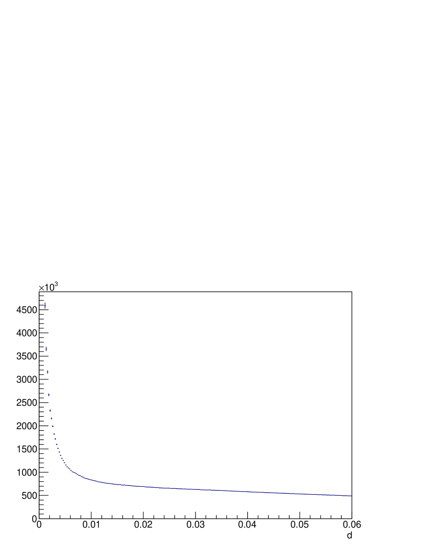
Figure 1: Histogram of the galaxy-galaxy BAO distances $d(z,z_{c})$ with weights $(0.033/d)^{2}$ for galaxy pairs with $d_{z}(z,z_{c})<d_{\alpha}(z,z_{c})/3$ corresponding to the entry with $z=0.54$ in Table 3. This histogram obtains $\hat{d}_{\alpha}(0.54,z_{c})$ as shown in Fig. 2. Note galaxy clustering at small $d$.

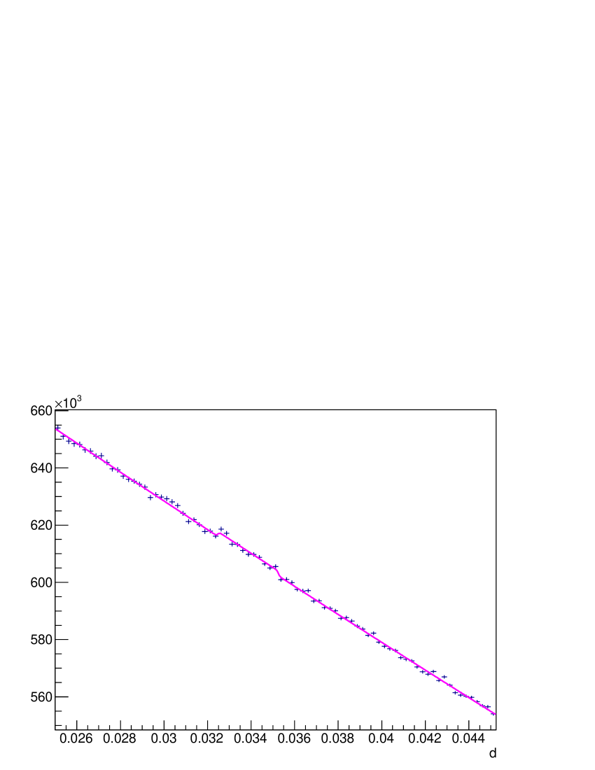
Figure 2: Detail of Fig. 1 with fit that obtains $\hat{d}_{\alpha}(0.54,z_{c})$. Note the fluctuations in the background due to galaxy clustering.

With few exceptions, we only accept runs with good fits for all three BAO distances $\hat{d}_{\alpha}(z,z_{c})$, $\hat{d}_{z}(z,z_{c})$, and $\hat{d}_{/}(z,z_{c})$ with consistent relative amplitudes and half-widths $\Delta d$ of the signal.

Final results of these BAO distance measurements are presented in Table 3. These 18 BAO distances are independent, do not depend on cosmological parameters, and are the main result of the present analysis. As cross-checks, and to estimate the systematic uncertainties, we present additional BAO distance measurements in Table 4.

V Systematic uncertainties

The backgrounds of BAO distance histograms have fluctuations due to the clustering of galaxies BH as seen in Fig. 2. These fluctuations are the dominant source of systematic uncertainties of the BAO distance measurements. These systematic effects are independent for each entry in Table 3. We estimate the systematic uncertainties directly from the data by calculating the standard deviations of measurements presented in Tables 3 and 4 with similar $z$ separately for $\hat{d}_{\alpha}(z,z_{c})$, $\hat{d}_{z}(z,z_{c})$, and $\hat{d}_{/}(z,z_{c})$. These measurements have different galaxy and center selections and different bins $(z_{\textrm{min}},z_{\textrm{max}})$ so the fluctuations of the backgrounds of the BAO distance histograms are different. The resulting standard deviations are approximately $0.00060$ for $\hat{d}_{\alpha}(z,z_{c})$, $\hat{d}_{z}(z,z_{c})$, and $\hat{d}_{/}(z,z_{c})$ independently of $z$, so we assign an independent systematic uncertainty $\pm 0.00060$ to each entry in Tables 3 and 4 to be summed in quadrature with the statistical uncertainties obtained from the fits. The histograms of BAO distances have a bin size $0.00025$ that is much smaller than the systematic uncertainty.

Here are two ideas left for future studies: (i) The systematic uncertainty $\pm 0.00060$ is about three times larger than the statistical uncertainties from the fits. Therefore it should be possible to improve the selection of galaxies and centers to reduce the systematic uncertainty at the expense of increasing the statistical uncertainties. (ii) For some bins in $z$ it was possible to fit several runs, e.g. G-G, LG-LG and G-C, which are partially independent, see Tables 3 and 4. Averaging such measurements may be considered.

Table 3: Independent measured BAO distances $\hat{d}_{\alpha}(z,z_{c})$, $\hat{d}_{z}(z,z_{c})$, and $\hat{d}_{/}(z,z_{c})$ in units of $c/H_{0}$ with $z_{c}=3.79$ (see text) from SDSS DR12 galaxies with right ascension $110^{0}$ to $260^{0}$ and declination $0^{0}$ to $70^{0}$. Uncertainties are statistical from the fits to the BAO signal. Each BAO distance has an independent systematic uncertainty $\pm 0.00060$. No corrections have been applied.

$z$	$z_{\textrm{min}}$	$z_{\textrm{max}}$	galaxies	centers	type	$\hat{d}_{\alpha}(z,z_{c})\times 100$	$\hat{d}_{z}(z,z_{c})\times 100$	$\hat{d}_{/}(z,z_{c})\times 100$
$0.10$	0.0	0.2	297220	5770	G-C	$3.338\pm 0.003$	$3.354\pm 0.006$	$3.361\pm 0.017$
$0.25$	0.2	0.3	56545	3552	G-LG	$3.454\pm 0.016$	$3.301\pm 0.008$	$3.432\pm 0.011$
$0.35$	0.3	0.4	78634	32095	G-LG	$3.318\pm 0.006$	$3.276\pm 0.013$	$3.410\pm 0.009$
$0.46$	0.4	0.5	124225	124225	G-G	$3.535\pm 0.013$	$3.494\pm 0.017$	$3.442\pm 0.036$
$0.54$	0.5	0.6	168766	168766	G-G	$3.385\pm 0.007$	$3.450\pm 0.019$	$3.547\pm 0.014$
$0.67$	0.6	0.9	95206	2617	G-C	$3.485\pm 0.019$	$3.471\pm 0.027$	$3.364\pm 0.070$

Table 4: Additional measured BAO distances $\hat{d}_{\alpha}(z,z_{c})$, $\hat{d}_{z}(z,z_{c})$, and $\hat{d}_{/}(z,z_{c})$ in units of $c/H_{0}$ with $z_{c}=3.79$ (see text) from SDSS DR12 galaxies with right ascension $110^{0}$ to $260^{0}$ and declination $0^{0}$ to $70^{0}$. Uncertainties are statistical from the fits to the BAO signal. Each BAO distance has an independent systematic uncertainty $\pm 0.00060$. No corrections have been applied.

$z$	$z_{\textrm{min}}$	$z_{\textrm{max}}$	galaxies	centers	type	$\hat{d}_{\alpha}(z,z_{c})\times 100$	$\hat{d}_{z}(z,z_{c})\times 100$	$\hat{d}_{/}(z,z_{c})\times 100$
$0.13$	0.1	0.2	175841	175841	G-G		$3.450\pm 0.012$
$0.25$	0.2	0.3	14699	4026	FG-C	$3.431\pm 0.015$
$0.25$	0.2	0.3	41846	4026	CG-C		$3.335\pm 0.010$	$3.389\pm 0.019$
$0.32$	0.2	0.4	135179	16446	G-C	$3.427\pm 0.014$	$3.413\pm 0.019$	$3.457\pm 0.011$
$0.35$	0.3	0.4	26130	5112	FG-C			$3.345\pm 0.018$
$0.38$	0.2	0.5	237651	25318	G-C	$3.388\pm 0.058$	$3.416\pm 0.016$	$3.404\pm 0.011$
$0.38$	0.2	0.5	259404	259404	G-G	$3.588\pm 0.014$	$3.329\pm 0.008$	$3.382\pm 0.009$
$0.38$	0.2	0.5	259404	28515	G-C		$3.413\pm 0.017$	$3.431\pm 0.008$
$0.41$	0.3	0.5	202859	45033	G-LG	$3.398\pm 0.060$	$3.318\pm 0.036$	$3.387\pm 0.009$
$0.46$	0.4	0.5	124225	12089	G-C	$3.501\pm 0.012$	$3.445\pm 0.033$	$3.435\pm 0.015$
$0.46$	0.4	0.5	68361	4945	FG-C	$3.337\pm 0.021$		$3.453\pm 0.015$
$0.54$	0.5	0.6	168766	11671	G-C	$3.429\pm 0.015$	$3.637\pm 0.026$	$3.627\pm 0.016$
$0.54$	0.5	0.6	168766	5553	G-LC	$3.373\pm 0.018$	$3.485\pm 0.010$	$3.423\pm 0.012$
$0.54$	0.5	0.6	168766	1608	G-C	$3.545\pm 0.034$	$3.568\pm 0.013$	$3.578\pm 0.054$
$0.54$	0.5	0.6	49102	4180	CG-C	$3.453\pm 0.013$	$3.404\pm 0.171$
$0.59$	0.5	0.9	263973	1959	G-C	$3.557\pm 0.028$	$3.531\pm 0.031$	$3.576\pm 0.026$
$0.59$	0.5	0.9	120927	120927	LG-LG	$3.414\pm 0.071$	$3.586\pm 0.083$	$3.530\pm 0.017$
$0.59$	0.5	0.9	263973	263973	G-G	$3.380\pm 0.008$	$3.560\pm 0.013$	$3.576\pm 0.011$
$0.67$	0.6	0.9	95206	95206	G-G	$3.397\pm 0.019$		$3.492\pm 0.009$
$0.67$	0.6	0.9	51310	51310	LG-LG	$3.469\pm 0.017$	$3.586\pm 0.018$	$3.459\pm 0.014$
$0.67$	0.6	0.9	95206	6741	G-C	$3.505\pm 0.020$		$3.459\pm 0.014$
$0.67$	0.6	0.9	109488	109488	G-G	$3.391\pm 0.121$	$3.549\pm 0.014$	$3.397\pm 0.025$

VI Corrections

Let us consider corrections to the BAO distances due to peculiar velocities and peculiar displacements of galaxies towards their centers. A relative peculiar velocity $v_{p}$ towards the center causes a reduction of the BAO distances $\hat{d}_{z}(z,z_{c})$, $\hat{d}_{/}(z,z_{c})$, and $\hat{d}_{\alpha}(z,z_{c})$ of order $v_{p}/c$. In addition, the Doppler shift produces an apparent shortening of $\hat{d}_{z}(z,z_{c})$ by $v_{p}/c$, and somewhat less for $\hat{d}_{/}(z,z_{c})$.

From the studies in Ref. Scoccimarro we add the following corrections to the measured BAO distances presented in Tables 3 and 4:

$$\Delta d_{z}=0.0012,\Delta d_{/}=0.75\Delta d_{z},\Delta d_{\alpha}=0.5\Delta d_{z}$$ (20)

respectively to $\hat{d}_{z}(z,z_{c})$, $\hat{d}_{/}(z,z_{c})$, and $\hat{d}_{\alpha}(z,z_{c})$. These corrections depend on $z$ and on the mass of the halos so $\Delta d_{z}$ lies in the approximate range 0.0006 to 0.0024 Scoccimarro .

We would like to obtain the peculiar motion corrections directly from the data. We exploit the fact that the corrections $\Delta d_{z}$ and $\Delta d_{\alpha}\approx 0.5\Delta d_{z}$ Scoccimarro are different so the correct $\Delta d_{z}$ should minimize the $\chi^{2}$ of fits. In Table 5 we present fits to the cosmological parameters $\Omega_{k}$, $\Omega_{\textrm{DE}}-0.5\Omega_{k}$ and $d_{\textrm{BAO}}$ that minimize the $\chi^{2}$ with 18 terms corresponding to the 18 entries in Table 3 for $\Delta d_{z}=0.0000$, $0.0012$, $0.0024$, and $0.0036$. The fits correspond to Scenario 4 with free $\Omega_{k}$. We present $\Omega_{\textrm{DE}}+0.5\Omega_{k}$ which has a smaller uncertainty than $\Omega_{\textrm{DE}}$. We observe that the $\chi^{2}$ of the fits is minimized at $\Delta d_{z}=0.0012\pm 0.0013$. The same result $\Delta d_{z}=0.0012\pm 0.0013$ is obtained for Scenario 1 with free $\Omega_{k}$. Minimizing the $\chi^{2}$ with 19 terms corresponding to the 18 BAO measurements plus the measurement of $\theta_{\textrm{MC}}$ in Scenario 4 with free $\Omega_{k}$ results in a minimum $\chi^{2}$ at $\Delta d_{z}=0.0018\pm 0.0008$.

Table 5: Cosmological parameters obtained from the 18 BAO measurements in Table 3 in Scenario 4, i.e. $\Omega_{\textrm{DE}}(a)=\Omega_{\textrm{DE}}\left[1+w_{1}(1-a)\right]$, for several peculiar motion corrections $\Delta d_{z}$, see Eq. (20). The minimum $\chi^{2}$ is obtained at $\Delta d_{z}=0.0012\pm 0.0013$.

	Scenario 4	Scenario 4	Scenario 4	Scenario 4
$\Delta d_{z}$	0.0000	0.0012	0.0024	0.0036
$\Omega_{k}$	$-0.560\pm 0.277$	$-0.235\pm 0.283$	$0.096\pm 0.288$	$0.433\pm 0.291$
$\Omega_{\textrm{DE}}+0.5\Omega_{k}$	$0.693\pm 0.066$	$0.656\pm 0.065$	$0.618\pm 0.064$	$0.581\pm 0.063$
$w_{1}$	$0.254\pm 0.612$	$0.132\pm 0.783$	$-0.085\pm 1.096$	$-0.558\pm 1.851$
$d_{\textrm{BAO}}\times 100$	$3.38\pm 0.06$	$3.45\pm 0.07$	$3.51\pm 0.07$	$3.57\pm 0.07$
$\chi^{2}/$d.f.	$19.4/14$	$18.6/14$	$19.3/14$	$21.3/14$

The distribution of the galaxies peculiar velocity component in one direction peaks at zero and drops to about 10% at $v_{p}\approx\pm 1000$ km/s BH corresponding to $v_{p}/c=0.0033$. Most of these galaxies at large $v_{p}$ are in clusters. For relative peculiar velocities of galaxies towards centers at the large BAO distance we expect $v_{p}/c\ll 0.0033$.

In the limit $z\rightarrow 0$ we obtain the corrected BAO distances $\hat{d}_{z}(0,z_{c})=\hat{d}_{\alpha}(0,z_{c})$. If from Scoccimarro we take approximately $\Delta d_{\alpha}\approx 0.5\Delta d_{z}$, we obtain $\Delta d_{z}\approx-0.0003\pm 0.0017$ from the row $z=0.1$ of Table 3, and $\Delta d_{z}\approx 0.0031\pm 0.0013$ from the row $z=0.25$, with an average $\Delta d_{z}\approx 0.0014\pm 0.0011$.

In conclusion, we apply to the entries of Tables 3 and 4 the corrections in Eqs. (20) with $\Delta d_{z}=0.0012\pm 0.0012$, which is coherent for all entries. In the next Section we present fits for $\Delta d_{z}=0.0012$ and $\Delta d_{z}=0.0000$.

Table 6: Cosmological parameters obtained from the 18 BAO measurements in Table 3 in several scenarios. Corrections for peculiar motions are given by Eq. (20) with the indicated $\Delta d_{z}$. Scenario 1 has $\Omega_{\textrm{DE}}$ constant. Scenario 2 has $w(a)=w_{0}+w_{a}(1-a)$. Scenario 3 has $w=w_{0}$. Scenario 4 has $\Omega_{\textrm{DE}}(a)=\Omega_{\textrm{DE}}\left[1+w_{1}(1-a)\right]$.

	Scenario 1	Scenario 1	Scenario 1	Scenario 2	Scenario 3	Scenario 4
$\Delta d_{z}$	0.0000	0.0012	0.0012	0.0012	0.0012	0.0012
$\Omega_{k}$	$0$ fixed	$0$ fixed	$-0.216\pm 0.257$	$-0.240\pm 0.283$	$-0.238\pm 0.283$	$-0.235\pm 0.283$
$\Omega_{\textrm{DE}}+0.5\Omega_{k}$	$0.660\pm 0.022$	$0.642\pm 0.022$	$0.646\pm 0.022$	$0.830\pm 0.797$	$0.663\pm 0.099$	$0.656\pm 0.065$
$w_{0}$	n.a.	n.a.	n.a.	$-0.821\pm 0.729$	$-0.948\pm 0.270$	n.a.
$w_{a}$ or $w_{1}$	n.a.	n.a.	n.a.	$0.754\pm 1.496$	n.a.	$0.132\pm 0.783$
$d_{\textrm{BAO}}\times 100$	$3.38\pm 0.03$	$3.44\pm 0.03$	$3.45\pm 0.03$	$3.45\pm 0.07$	$3.45\pm 0.06$	$3.45\pm 0.07$
$\chi^{2}/$d.f.	$23.4/16$	$19.3/16$	$18.6/15$	$18.5/13$	$18.6/14$	$18.6/14$

Table 7: Cosmological parameters obtained from the 18 BAO measurements in Table 3 plus $\theta_{\textrm{MC}}$ from Eq. (12) in several scenarios. Corrections for peculiar motions are given by Eq. (20) with $\Delta d_{z}=0.0012$. Scenario 1 has $\Omega_{\textrm{DE}}$ constant. Scenario 2 has $w(a)=w_{0}+w_{a}(1-a)$. Scenario 3 has $w=w_{0}$. Scenario 4 has $\Omega_{\textrm{DE}}(a)=\Omega_{\textrm{DE}}\left[1+w_{1}(1-a)\right]$.

	Scenario 1	Scenario 1	Scenario 2	Scenario 3	Scenario 4	Scenario 4
$\Delta d_{z}$	$0.0012$	$0.0012$	$0.0012$	$0.0012$	$0.0012$	$0.0012$
$\Omega_{k}$	$0$ fixed	$0.061\pm 0.012$	$0$ fixed	$0$ fixed	$0$ fixed	$0.065\pm 0.043$
$\Omega_{\textrm{DE}}+2\Omega_{k}$	$0.754\pm 0.004$	$0.733\pm 0.005$	$0.808\pm 0.075$	$0.745\pm 0.004$	$0.732\pm 0.006$	$0.734\pm 0.008$
$w_{0}$	n.a.	n.a.	$-0.795\pm 0.092$	$-0.730\pm 0.046$	n.a.	n.a.
$w_{a}$ or $w_{1}$	n.a.	n.a.	$0.705\pm 0.170$	n.a.	$1.157\pm 0.245$	$-0.113\pm 0.985$
$d_{\textrm{BAO}}\times 100$	$3.58\pm 0.02$	$3.44\pm 0.03$	$3.44\pm 0.04$	$3.40\pm 0.04$	$3.37\pm 0.04$	$3.45\pm 0.06$
$\chi^{2}/$d.f.	$52.2/17$	$19.7/16$	$19.4/15$	$20.4/16$	$22.1/16$	$19.7/15$

Table 8: Cosmological parameters obtained from the 18 BAO measurements in Table 3 plus $\theta_{\textrm{MC}}$ from Eq. (12) in several scenarios. No corrections for peculiar motions are applied. Scenario 1 has $\Omega_{\textrm{DE}}$ constant. Scenario 2 has $w(a)=w_{0}+w_{a}(1-a)$. Scenario 3 has $w=w_{0}$. Scenario 4 has $\Omega_{\textrm{DE}}(a)=\Omega_{\textrm{DE}}\left[1+w_{1}(1-a)\right]$.

	Scenario 1	Scenario 1	Scenario 2	Scenario 3	Scenario 4	Scenario 4
$\Delta d_{z}$	$0.0000$	$0.0000$	$0.0000$	$0.0000$	$0.0000$	$0.0000$
$\Omega_{k}$	$0$ fixed	$0.037\pm 0.011$	$0$ fixed	$0$ fixed	$0$ fixed	$0.043\pm 0.041$
$\Omega_{\textrm{DE}}+2\Omega_{k}$	$0.733\pm 0.004$	$0.716\pm 0.006$	$0.777\pm 0.087$	$0.724\pm 0.005$	$0.718\pm 0.006$	$0.716\pm 0.006$
$w_{0}$	n.a.	n.a.	$-0.906\pm 0.110$	$-0.817\pm 0.051$	n.a.	n.a.
$w_{a}$ or $w_{1}$	n.a.	n.a.	$0.825\pm 0.279$	n.a.	$0.729\pm 0.237$	$-0.161\pm 0.941$
$d_{\textrm{BAO}}\times 100$	$3.46\pm 0.02$	$3.38\pm 0.03$	$3.39\pm 0.05$	$3.35\pm 0.04$	$3.34\pm 0.04$	$3.39\pm 0.06$
$\chi^{2}/$d.f.	$36.5/17$	$23.9/16$	$23.2/15$	$24.3/16$	$25.0/16$	$23.9/15$

VII Cosmological parameters from BAO

Let us try to understand qualitatively how the BAO distance measurements presented in Table 3 constrain the cosmological parameters. In the limit $z\rightarrow 0$ we obtain $d_{\textrm{BAO}}=\hat{d}_{\alpha}(0,z_{c})=\hat{d}_{z}(0,z_{c})=\hat{d}_{/}(0,z_{c})$, so the row with $z=0.1$ in Table 3 approximately determines $d_{\textrm{BAO}}$. This $d_{\textrm{BAO}}$ and the measurement of, for example, $\hat{d}_{z}(0.3,z_{c})$ then constrains the derivative of $\Omega_{\textrm{m}}/a^{3}+\Omega_{\textrm{DE}}+\Omega_{\textrm{k}}/a^{2}$ with respect to $a$ at $z\approx 0.3$, i.e. constrains approximately $\Omega_{\textrm{DE}}+0.5\Omega_{k}$ or equivalently $\Omega_{\textrm{DE}}-\Omega_{\textrm{m}}$. The fit to the BAO data of Table 3 for Scenario 1 (with the correction (20) with $\Delta d_{z}=0.0012$) obtains $\Omega_{\textrm{DE}}+0.5\Omega_{k}=0.646\pm 0.022$, while the constraint on the orthogonal relation is quite weak: $\Omega_{\textrm{DE}}-2.0\Omega_{k}=1.184\pm 0.682$. We need an additional constraint for Scenario 1. At small $a$, $E(a)$ is dominated by $\Omega_{\textrm{m}}$, so $\theta_{\textrm{MC}}$ plus $d_{\textrm{BAO}}$ approximately constrain $\Omega_{\textrm{m}}$, or equivalently $\Omega_{\textrm{DE}}+\Omega_{k}$, see Eq. (19). The additional BAO distance measurements in Table 3 then also constrain $w_{0}$ and $w_{a}$ or $w_{1}$.

In Table 6 we present the cosmological parameters obtained by minimizing the $\chi^{2}$ with 18 terms corresponding to the 18 BAO distance measurements in Table 3 for several scenarios. We find that the data (with the correction (20) with $\Delta d_{z}=0.0012$) is in agreement with the simplest cosmology with $\Omega_{k}=0$ and $\Omega_{\textrm{DE}}(a)$ constant with $\chi^{2}$ per degree of freedom (d.f.) $19.3/16$, so no additional parameter is needed to obtain a good fit to this data. Note that the BAO data alone place a tight constraint on $\Omega_{\textrm{DE}}+0.5\Omega_{k}=0.646\pm 0.022$ for constant $\Omega_{\textrm{DE}}(a)$, or $0.656\pm 0.065$ when $\Omega_{\textrm{DE}}(a)$ is allowed to depend on $a$ as in Scenario 4. The constraint on $\Omega_{k}$ is weak.

In Table 7 we present the cosmological parameters obtained by minimizing the $\chi^{2}$ with 19 terms corresponding to the 18 BAO distance measurements listed in Table 3 (with the correction (20) with $\Delta d_{z}=0.0012$) plus the measurement of $\theta_{\textrm{MC}}$ from the CMB given in Eq. (12). We present the variable $\Omega_{\textrm{DE}}+2\Omega_{\textrm{k}}$ instead of $\Omega_{\textrm{DE}}$ because it has a smaller uncertainty. The simplest cosmology with $\Omega_{k}=0$ and $\Omega_{\textrm{DE}}(a)$ constant has $\chi^{2}$ per d.f. $52.2/17$ and is therefore disfavored with a significance corresponding to $4.3\sigma$ for one degree of freedom. Releasing one of the parameters $\Omega_{k}$ or $w_{0}$ or $w_{1}$ obtains a good fit to the data. Releasing only $\Omega_{k}$ obtains $\Omega_{k}=0.061\pm 0.012$ with $\chi^{2}$ per d.f. $19.7/16$. Releasing only $w_{0}$ obtains $w_{0}=-0.730\pm 0.046$ with $20.4/16$. Releasing only $w_{1}$ obtains $w_{1}=1.157\pm 0.245$ with $22.1/16$. Releasing both $\Omega_{k}$ and $w_{1}$ obtains $\chi^{2}$ per d.f. $19.7/15$, $\Omega_{k}=0.065\pm 0.043$ and $w_{1}=-0.113\pm 0.985$. Details of these and other fits are presented in Table 7. Table 8 presents the corresponding fits with no correction for peculiar motions.

In summary, we find that the BAO$+\theta_{\textrm{MC}}$ data are in agreement with a family of universes with different $\Omega_{k}$. Two examples are presented in Table 7: see the fits for Scenario 4. Fixing $\Omega_{k}=0.065$ we obtain $\Omega_{\textrm{DE}}$ independent of $a$ within uncertainties: $w_{1}=-0.105\pm 0.279$. Fixing $\Omega_{k}=0$ we obtain $\Omega_{\textrm{DE}}(a)$ that does depend significantly on $a$: $w_{1}=1.157\pm 0.245$. However, if we require both $\Omega_{k}=0$ and $\Omega_{\textrm{DE}}(a)$ constant we obtain disagreement with the data with $\chi^{2}$ per d.f. $52.2/17$.

VIII Cross-checks

The reference fit in this Section is Scenario 1 with $\Omega_{k}=0$ fixed, $\chi^{2}$ with 19 terms: 18 BAO terms from Table 3 (corrected with $\Delta d_{z}=0.0012$) plus $\theta_{\textrm{MC}}$ from Eq. (12). The $\chi^{2}$ per d.f. is $52.2/17$, see Table 7. This tension is equivalent to $4.3\sigma$ for one degree of freedom. Releasing a single parameter reduces the tension to less than $1.5\sigma$.

The main contributions to the $\chi^{2}$ of the reference fit are $\hat{d}_{/}(0.54,z_{c})$ contributing 8.5, $\hat{d}_{z}(0.46,z_{c})$, $\hat{d}_{z}(0.67,z_{c})$, $\hat{d}_{\alpha}(0.10,z_{c})$, $\hat{d}_{z}(0.54,z_{c})$, and $\hat{d}_{\alpha}(0.35,z_{c})$ contributing 4.7. So we see no obvious pattern or mistake in the identification of the BAO signals.

Removing the term corresponding to $\theta_{\textrm{MC}}$ from the $\chi^{2}$ obtains $19.3/16$, so the tension is between the $\theta_{\textrm{MC}}$ measurement and the BAO measurements. Does $\theta_{\textrm{MC}}$ need a correction?

Here are fits with less BAO terms in the $\chi^{2}$ than the reference fit. Fitting the 6 $\hat{d}_{z}(z,z_{c})$ measurements plus $\theta_{\textrm{MC}}$ obtains $23.7/5$. Fitting the 6 $\hat{d}_{\alpha}(z,z_{c})$ measurements plus $\theta_{\textrm{MC}}$ obtains $13.7/5$. Fitting the 6 $\hat{d}_{/}(z,z_{c})$ measurements plus $\theta_{\textrm{MC}}$ obtains $11.0/5$. Removing $\hat{d}_{\alpha}(0.10,z_{c})$ obtains $44.7/16$. Removing the 3 BAO entries with $z=0.1$ obtains $39.0/14$. Removing the 3 BAO entries with $z=0.67$ obtains $42.4/14$. Removing the 6 BAO entries with $z=0.1$ and $z=0.25$ obtains $35.3/11$. Removing the 6 BAO entries with $z=0.54$ and $z=0.67$ obtains $26.0/11$. In conclusion, none of these removals of BAO measurements from the $\chi^{2}$ of the fit removes the tension.

We now perform a fit with different BAO measurements listed in Table 4: $0.2<z<0.4$ G-C, $0.4<z<0.5$ G-C, $0.5<z<0.6$ G-LC, and $0.6<z<0.9$ LG-LG. These measurements have different selections of centers and/or galaxies, or different binnings of $z$, and different fits from the measurements in Table 3. The fit to these 12 BAO measurements plus $\theta_{\textrm{MC}}$ for Scenario 1 with $\Omega_{k}=0$ fixed obtains $32.0/11$, equivalent to a tension of $3.4\sigma$ for 1 degree of freedom. Releasing only $\Omega_{k}$ obtains $4.6/10$ with $\Omega_{k}=0.072\pm 0.017$. Releasing only $w_{0}$ obtains $5.9/10$ with $w_{0}=-0.658\pm 0.065$. Releasing only $w_{1}$ obtains $7.2/10$ with $w_{1}=1.745\pm 0.458$. Note that releasing a single parameter removes the tension. These last three fits are consistent with the ones presented in Table 7, and have $\chi^{2}$ per d.f. less than 1 confirming that we are not underestimating the systematic uncertainty of the BAO distances.

To remove the tension between the Scenario with $\Omega_{k}=0$ fixed and $\Omega_{\textrm{DE}}(a)$ constant it is necessary to shift $\theta_{\textrm{MC}}$ by $200\sigma$ or increase the systematic uncertainty of the BAO distances $\pm 0.00060$ by a factor 1.7. It is difficult to imagine that the systematic uncertainty is wrong by a factor 1.7 when it was obtained directly from the data, and in addition we obtain $\chi^{2}$ per d.f. close to 1 by releasing a single parameter.

The conclusions are: (i) Scenario 1 with $\Omega_{k}=0$ and constant $\Omega_{\textrm{DE}}(a)$ has tension with the BAO plus $\theta_{\textrm{MC}}$ data, and (ii) dropping the constraint $\Omega_{k}=0$ and/or allowing $\Omega_{\textrm{DE}}(a)$ to be variable leaves no significant tension. These conclusions are robust with respect to the selection of the BAO data.

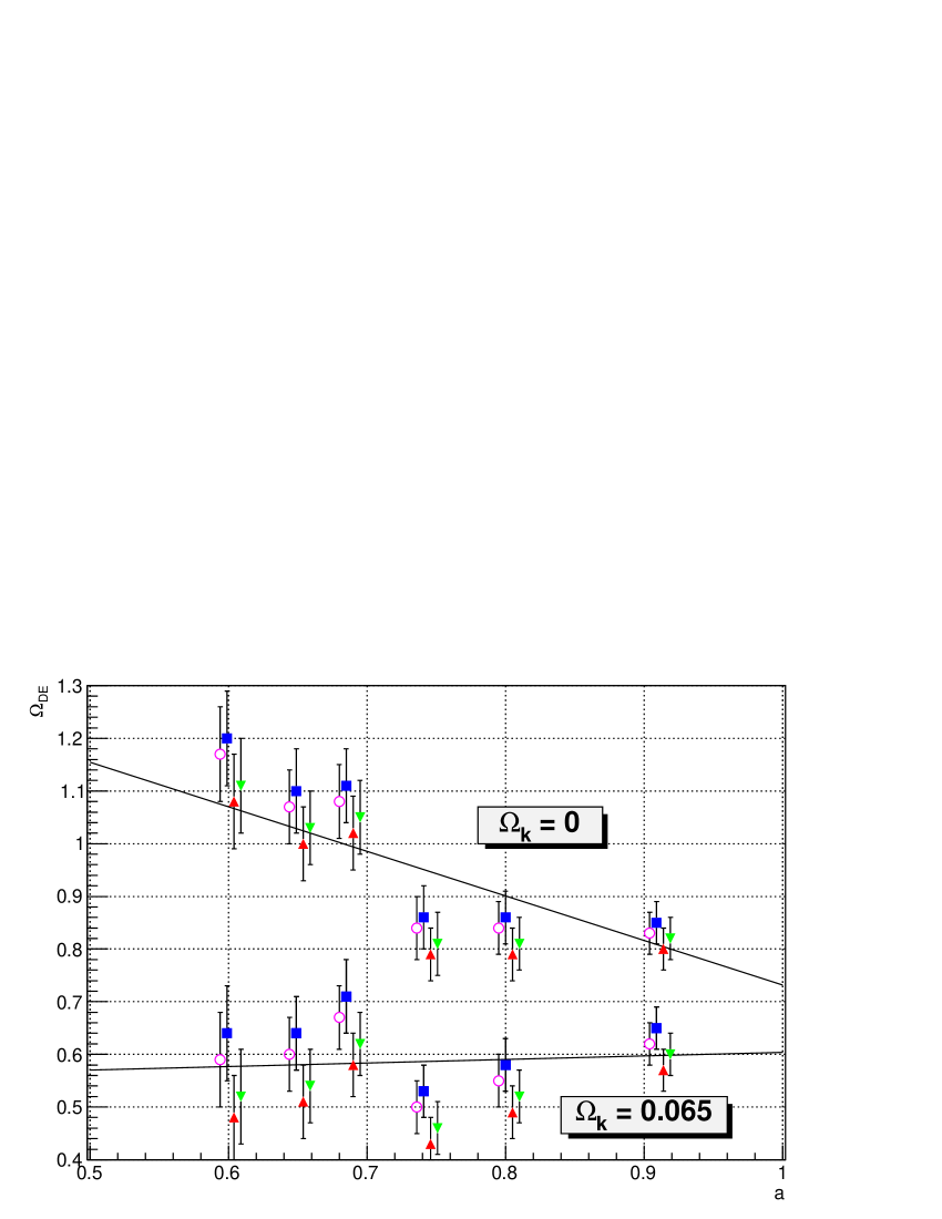
Figure 3: Measurements of $\Omega_{\textrm{DE}}(a)$ obtained from the 6 $\hat{d}_{z}(z,z_{c})$ in Table 3 for $\Omega_{k}=0$ and $\Omega_{k}=0.065$, and the corresponding $d_{\textrm{BAO}}$ and $\Omega_{\textrm{DE}}$ from the fits for Scenario 4 in Table 7. The straight lines are $\Omega_{\textrm{DE}}=0.732\left[1+1.157(1-a)\right]$ and $\Omega_{\textrm{DE}}=0.604\left[1-0.113(1-a)\right]$ from these fits. The uncertainties correspond only to the total uncertainties of $\hat{d}_{z}(z,z_{c})$. For clarity some offsets in $a$ have been applied. For $\Omega_{k}=0$ we have $(d_{\textrm{BAO}},\Omega_{\textrm{DE}})=(0.0337-0.0004,0.732)$ (squares), $(0.0337+0.0004,0.732)$ (triangles), $(0.0337,0.732-0.006)$ (inverted triangles), $(0.0337,0.732+0.006)$ (circles). For $\Omega_{k}=0.065$ we have $(0.0345-0.0006,0.604)$ (squares), $(0.0345+0.0006,0.604)$ (triangles), $(0.0345,0.604-0.008)$ (inverted triangles), $(0.0345,0.604+0.008)$ (circles).

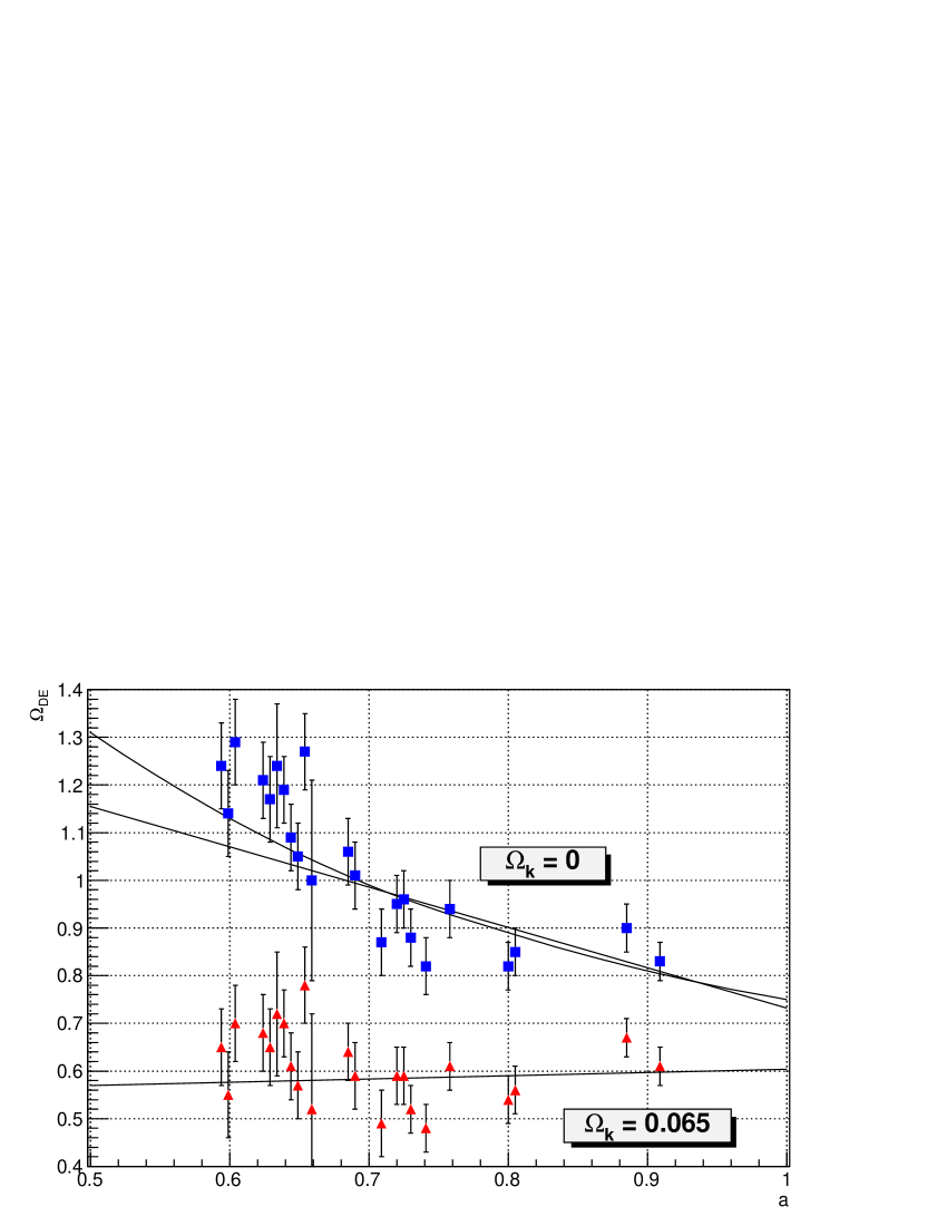
Figure 4: Same as Figure 3 with the addition of the 17 measurements of $\hat{d}_{z}(z,z_{c})$ in Table 4. These measurements are partially correlated. For $\Omega_{k}=0$ we have $(d_{\textrm{BAO}},\Omega_{\textrm{DE}})=(0.0337,0.732)$ (squares). For $\Omega_{k}=0.065$ we have $(0.0345,0.604)$ (triangles). The curve corresponding to the fit for Scenario 3 in Table 7 has been added.

IX Measurement of $\Omega_{\textrm{DE}}(a)$

We obtain $\Omega_{\textrm{DE}}(a)$ from the 6 independent measurements of $\hat{d}_{z}(z,z_{c})$ in Table 3 with the correction $\Delta d_{z}=0.0012$ and Eqs. (17) and (2), for the cases $\Omega_{k}=0.065$ and $\Omega_{k}=0$. The values of $d_{\textrm{BAO}}$ and $\Omega_{\textrm{DE}}$ are obtained from the fits for Scenario 4 in Table 7. The results are presented in Fig. 3. To guide the eye, we also show the straight line corresponding to Scenario 4.

To cross-check the robustness of $\Omega_{\textrm{DE}}(a)$ in Fig. 3 we add the 17 measurements of $\hat{d}_{z}(z,z_{c})$ in Table 4 and obtain Fig. 4. Note that these measurements of $\hat{d}_{z}(z,z_{c})$ are partially correlated.

Note that $\Omega_{\textrm{DE}}(a)$ is consistent with a constant for $\Omega_{k}=0.065$, but not for $\Omega_{k}=0$.

X Conclusions

The main results of these studies are the 18 independent BAO distance measurements presented in Table 3 which do not depend on any cosmological parameter. These BAO distance measurements alone place a strong constraint on $\Omega_{\textrm{DE}}+0.5\Omega_{k}=0.646\pm 0.022$ (for constant $\Omega_{\textrm{DE}}$) or $0.656\pm 0.065$ (when $\Omega_{\textrm{DE}}(a)$ is allowed to depend on $a$), while the constraint on $\Omega_{k}$ is weak.

Constraints on the cosmological parameters in several scenarios from the BAO measurements alone and from BAO plus $\theta_{\textrm{MC}}$ measurements are presented in Tables 6, 7 and 8. We find that the 18 BAO distance measurements plus $\theta_{\textrm{DE}}$ are in agreement with a family of universes with different $\Omega_{k}$. Two examples are $\Omega_{k}=0.065$ with $\Omega_{\textrm{DE}}(a)$ constant, and $\Omega_{k}=0$ with $\Omega_{\textrm{DE}}(a)$ varying significantly with $a$. For these two examples we present measurements of $\Omega_{\textrm{DE}}(a)$ in Figs. 3 and 4. The cosmology with both $\Omega_{k}=0$ and $\Omega_{\textrm{DE}}(a)$ constant has a tension of $4.3\sigma$ with the BAO plus $\theta_{\textrm{MC}}$ data.

The BAO plus $\theta_{\textrm{MC}}$ data for constant $\Omega_{\textrm{DE}}(a)$ obtains $\Omega_{k}=0.061\pm 0.012$ for $\Delta d_{z}=0.0012$ and $\Omega_{k}=0.037\pm 0.011$ for $\Delta d_{z}=0$. These results have some tension with independent observations: $\Omega_{k}=-0.042^{+0.024}_{-0.022}$ from CMB data alone with the assumption of constant $\Omega_{\textrm{DE}}(a)$ PDG , and $\Omega_{k}\approx 0.000\pm 0.013$ from CMB plus supernova (SN) data with the assumption of constant $\Omega_{\textrm{DE}}(a)$ PDG . If $\Omega_{\textrm{DE}}(a)$ is allowed to be variable there are only loose constraints on $\Omega_{k}$ from independent measurements, so the case with $\Omega_{k}=0$ with non-constant $\Omega_{\textrm{DE}}(a)$ is viable.

XI Acknowledgment

Funding for SDSS-III has been provided by the Alfred P. Sloan Foundation, the Participating Institutions, the National Science Foundation, and the U.S. Department of Energy Office of Science. The SDSS-III web site is http://www.sdss3.org/.

SDSS-III is managed by the Astrophysical Research Consortium for the Participating Institutions of the SDSS-III Collaboration including the University of Arizona, the Brazilian Participation Group, Brookhaven National Laboratory, Carnegie Mellon University, University of Florida, the French Participation Group, the German Participation Group, Harvard University, the Instituto de Astrofisica de Canarias, the Michigan State/Notre Dame/JINA Participation Group, Johns Hopkins University, Lawrence Berkeley National Laboratory, Max Planck Institute for Astrophysics, Max Planck Institute for Extraterrestrial Physics, New Mexico State University, New York University, Ohio State University, Pennsylvania State University, University of Portsmouth, Princeton University, the Spanish Participation Group, University of Tokyo, University of Utah, Vanderbilt University, University of Virginia, University of Washington, and Yale University.

The author acknowledges the use of computing resources of Universidad de los Andes, Bogotá, Colombia.

References

- (1) D. J. Eisenstein, H.-J. Seo, and M. White, ApJ, 664: 660-674 (2007).
- (2) Bruce A. Bassett and Renée Hlozek, arXiv:0910.5224 (2009).
- (3) David H. Weinberg et.al., arXiv:1201.2434 (2013).
- (4) B. Hoeneisen, arXiv:astro-ph/0009071 (2000).
- (5) Shadab Alam, et al. (SDSS-III), arXiv:1501.00963 (2015).
- (6) K.A. Olive et al. (Particle Data Group). Chin. Phys. C, 2014, 38(9): 090001.
- (7) Eric V. Linder, Phys.Rev.Lett. 90:091301 (2003)
- (8) R.E. Smith, R. Scoccimarro, and R.K. Sheth, Phys. Rev. D, 75 (6): 063512 (2007). arXiv astro-ph/0703620.