Diclique clustering in a directed random graph

Abstract

We discuss a notion of clustering for directed graphs, which describes how likely two followers of a node are to follow a common target. The associated network motifs, called dicliques or bi-fans, have been found to be key structural components in various real-world networks. We introduce a two-mode statistical network model consisting of actors and auxiliary attributes, where an actor $i$ decides to follow an actor $j$ whenever $i$ demands an attribute supplied by $j$. We show that the digraph admits nontrivial clustering properties of the aforementioned type, as well as power-law indegree and outdegree distributions.

1 Introduction

1.1 Clustering in directed networks

Many real networks display a tendency to cluster, that is, to form dense local neighborhoods in a globally sparse graph. In an undirected social network this may be phrased as: your friends are likely to be friends. This feature is typically quantified in terms of local and global clustering coefficients measuring how likely two neighbors of a node are neighbors [11, 13, 14, 16]. In directed networks there are many ways to define the concept of clustering, for example by considering the thirteen different ways that a set of three nodes may form a weakly connected directed graph [5].

In this paper we discuss a new type of clustering concept which is motivated by directed online social networks, where a directed link $i\to j$ means that an actor $i$  follows actor $j$. In such networks a natural way to describe clustering is to say that your followers are likely to follow common targets. When the topology of the network is unknown and modeled as a random graph distributed according to a probability measure $P$, the above statement can be expressed as

$$P(i_{2}\to i_{4}\,\bigr{|}\,i_{1}\to i_{2},\,i_{1}\to i_{3},\,i_{2}\to i_{3})\ >\ P(i_{2}\to i_{4}),$$ (1)

where ’you’ corresponds to actor $i_{3}$. Interestingly, the conditional probability on the left can stay bounded away from zero even for sparse random digraphs [9]. The associated subgraph (Fig. 1) is called a diclique. Earlier experimental studies have observed that dicliques (a.k.a. bi-fans) constitute a key structural motif in gene regulation networks [10], citation networks, and several types of online social networks [17].

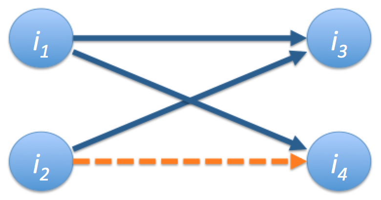
Figure 1: Forming a diclique by adding a link $i_{2}\to i_{4}$.

Motivated by the above discussion, we define a global diclique clustering coefficient of a finite directed graph $D$ with an adjacency matrix $(D_{ij})$ by

$${\cal C}_{\rm di}(D)=\frac{\sum_{(i_{1},i_{2},i_{3},i_{4})}D_{i_{1},i_{3}}D_{i_{1},i_{4}}D_{i_{2},i_{3}}D_{i_{2},i_{4}}}{\sum_{(i_{1},i_{2},i_{3},i_{4})}D_{i_{1},i_{3}}D_{i_{1},i_{4}}D_{i_{2},i_{3}}},$$ (2)

where the sums are computed over all ordered quadruples of distinct nodes. It provides an empirical counterpart to the conditional probability (1) in the sense that the ratio in (2) defines the conditional probability

$$P_{D}\bigl{(}I_{2}\to I_{4}\,\,\bigl{|}\,\,I_{1}\to I_{3},\,I_{1}\to I_{4},\,I_{2}\to I_{3}\bigr{)},$$ (3)

where $P_{D}$ refers to the distribution of the random quadruple $(I_{1},I_{2},I_{3},I_{4})$ sampled uniformly at random among all ordered quadruples of distinct nodes in $D$.

To quantify diclique clustering among the followers of a selected actor $i$, we may define a local diclique clustering coefficient by

$${\cal C}_{\rm di}(D,i)=\frac{\sum_{(i_{1},i_{2},i_{4})}D_{i_{1},i}D_{i_{1},i_{4}}D_{i_{2},i}D_{i_{2},i_{4}}}{\sum_{(i_{1},i_{2},i_{4})}D_{i_{1},i}D_{i_{1},i_{4}}D_{i_{2},i}},$$ (4)

where the sums are computed over all ordered triples of distinct nodes excluding $i$. We remark that ${\cal C}_{\rm di}(D,i)=P_{D}\bigl{(}I_{2}\to I_{4}\,\bigl{|}\,I_{1}\to I_{3},I_{1}\to I_{4},I_{2}\to I_{3},\,I_{3}=i\bigr{)}$.

Remark 1

By replacing $\to$ by $\leftrightarrow$ in (3), we see that the analogue of the above notion for undirected graphs corresponds to predicting how likely the endpoints of the 3-path $I_{2}\leftrightarrow I_{3}\leftrightarrow I_{1}\leftrightarrow I_{4}$ are linked together.

1.2 A directed random graph model

Our goal is to define a parsimonious yet powerful statistical model of a directed social network which displays diclique clustering properties as discussed in the previous section. Clustering properties in many social networks, such as movie actor networks or scientific collaboration networks, are explained by underlying bipartite structures relating actors to movies and scientists to papers [7, 12]. Such networks are naturally modeled using directed or undirected random intersection graphs [1, 3, 4, 6, 8].

A directed intersection graph on a node set $V=\{1,\dots,n\}$ is constructed with the help of an auxiliary set of attributes $W=\{w_{1},\dots,w_{m}\}$ and a directed bipartite graph $H$ with bipartition $V\cup W$, which models how nodes (or actors) relate to attributes. We say that actor $i$ demands (or follows) attribute $w_{k}$ when $i\to w_{k}$, and supplies it when $i\leftarrow w_{k}$. The directed intersection graph $D$ induced by $H$ is the directed graph on $V$ such that $i\to j$ if and only if $H$ contains a path $i\to w_{k}\to j$, or equivalently, $i$ demands one or more attributes supplied by $j$ (see Fig. 2). For example, in a citation network the fact that an author $i$ cites a paper $w_{k}$ coauthored by $j$, corresponds to $i\to w_{k}\to j$.

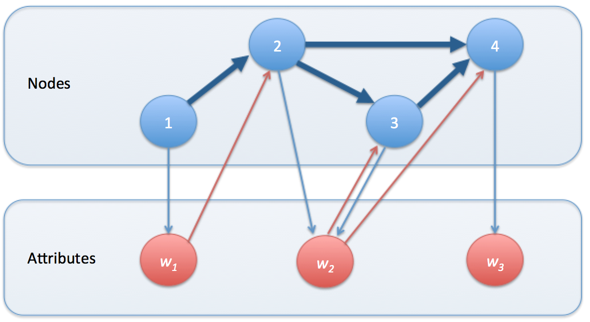
Figure 2: Node 1 follows node 2, because 1 demands attribute $w_{1}$ supplied by 2.

We consider a random bipartite digraph $H$ where the pairs $(i,w_{k})$, $i\in V$, $w_{k}\in W$ establish adjacency relations independently of each other. That is, the bivariate binary random vectors $({\mathbb{I}}_{i\to k},\,{\bf I}_{k\to i})$, $1\leq i\leq n$, $1\leq k\leq m$, are stochastically independent. Here ${\mathbb{I}}_{i\to k}$ and ${\bf I}_{k\to i}$ stand for the indicators of the events that links $i\to w_{k}$ and $w_{k}\to i$ are present in $H$. We assume that every pair $(i,w_{k})$ is assigned a triple of probabilities

$$p_{ik}=P(i\to w_{k}),\quad\ q_{ik}=P(w_{k}\to i),\quad\ r_{ik}=P(i\to w_{k},\,w_{k}\to i).$$ (5)

Note that, by definition, $r_{ik}$ satisfies the inequalities

$$\max\{p_{ik}+q_{ik}-1,0\}\ \leq\ r_{ik}\ \leq\ \min\{p_{ik},q_{ik}\}.$$ (6)

A collection of triples $\{(p_{ik},\,q_{ik},\,r_{ik}),\,1\leq i\leq n,\,1\leq k\leq m\}$ defines the distribution of a random bipartite digraph $H$.

We will focus on a fitness model where every node $i$ is prescribed a pair of weights $x_{i},y_{i}\geq 0$ modelling the demand and supply intensities of $i$. Similarly, every attribute $w_{k}$ is prescribed a weight $z_{k}>0$ modelling its relative popularity. Letting

$$p_{ik}=\min\Bigl{\{}1,\gamma x_{i}z_{k}\Bigr{\}}\qquad{\text{and}}\qquad q_{ik}=\min\Bigl{\{}1,\gamma y_{i}z_{k}\Bigr{\}},\qquad i,k\geq 1,$$ (7)

we obtain link probabilities proportional to respective weights. Furthermore, we assume that

$$r_{ik}=r(x_{i},y_{i},z_{k},\gamma),\qquad i,k\geq 1,$$ (8)

for some function $r\geq 0$ satisfying (6). Here $\gamma>0$ is a parameter, defining the link density in $H$, which generally depends on $m$ and $n$. Note that $r$ defines the correlation between reciprocal links $i\to w_{k}$ and $w_{k}\to i$. For example, by letting $r(x,y,z,\gamma)=(\gamma xz\wedge 1)(\gamma yz\wedge 1)$, we obtain a random bipartite digraph with independent links.

We will consider weight sequences having desired statistical properties for complex network modelling. For this purpose we assume that the node and attributes weights are realizations of random sequences $X=(X_{i})_{i\geq 1}$, $Y=(Y_{i})_{i\geq 1}$, and $Z=(Z_{k})_{k\geq 1}$, such that the sequences $\{(X_{i},Y_{i}),\,i\geq 1\}$ and $\{Z_{k},\,k\geq 1\}$ are mutually independent and consist of independent and identically distributed terms. The resulting random bipartite digraph is denoted by ${\cal H}$, and the resulting random intersection digraph by ${\cal D}$. We remark that ${\cal D}$ extends the random intersection digraph model introduced in [1].

1.3 Degree distributions

When $\gamma=(mn)^{-1/2}$ and $m,n\to\infty$, the random digraph ${\cal D}$ defined in Sec. 1.2 becomes sparse, having the number of links proportional to the number of nodes. Theorem 1.1 below describes the class of limiting distributions of the outdegree of a typical vertex $i$. We remark that for each $n$ the outdegrees $d_{+}(1)$,…, $d_{+}(n)$ are identically distributed.

To state the theorem, we let $\Lambda_{1},\Lambda_{2},\Lambda_{3}$ be mixed-Poisson random variables distributed according to

$$P(\Lambda_{i}=r)\ =\ E\,\,e^{-\lambda_{i}}\frac{\lambda_{i}^{r}}{r!},\quad r\geq 0,$$

where $\lambda_{1}=X_{1}\beta^{1/2}E\,Z_{1}$, $\lambda_{2}=Z_{1}\beta^{-1/2}E\,Y_{1}$, and $\lambda_{3}=X_{1}(E\,Y_{1})(E\,Z_{1}^{2})$. We also denote by $\Lambda_{i}^{*}$ a downshifted size-biased version of $\Lambda_{i}$, distributed according to

$$P(\Lambda_{i}^{*}=r)\ =\ \frac{r+1}{E\,\Lambda_{i}}P(\Lambda_{i}=r+1),\quad r\geq 0.$$

Below $\xrightarrow{d}$ refers to convergence in distribution.

Theorem 1.1

Consider a model with $n,m\to\infty$ and $\gamma=(nm)^{-1/2}$, and assume that $E\,Y_{1},E\,Z_{1}^{2}<\infty$.

1. If $m/n\to 0$ then $d_{+}(1)\xrightarrow{d}0$.

2. If $m/n\to\beta$ for some $\beta\in(0,\infty)$, then $d_{+}(1)\xrightarrow{d}\sum_{j=1}^{\Lambda_{1}}\Lambda_{2,j}^{*},$ where $\Lambda_{2,1}^{*},\Lambda_{2,2}^{*},\dots$ are independent copies of $\Lambda_{2}^{*}$, and independent of $\Lambda_{1}$.

3. If $m/n\to\infty$, then $d_{+}(1)\xrightarrow{d}\Lambda_{3}$.

Remark 2

By symmetry, the results of Theorem 1.1 extend to the indegree $d_{-}(1)$ when we redefine $\lambda_{1}=Y_{1}\beta^{1/2}E\,Z_{1}$, $\lambda_{2}=Z_{1}\beta^{-1/2}E\,X_{1}$, and $\lambda_{3}=Y_{1}(E\,X_{1})(E\,Z_{1}^{2})$.

Remark 3

The limiting distributions appearing in Theorem 1.1:(ii)–(iii) admit heavy tails. This random digraph model is rich enough to model power-law indegree and outdegree distributions, or power-law indegree and light-tailed outdegree distributions.

Remark 4

The moment conditions in Theorem 1.1 are not the sharpest possible. For example, in (i) it is sufficient to assume that $E\,Z_{1}<\infty$.

We note that a related result for simple (undirected) random intersection graph has been shown in [2]. Theorem 1.1 extends the result of [2] to digraphs.

1.4 Diclique clustering

We investigate clustering in the random digraph ${\cal D}$ defined in Sec. 1.2 by approximating the (random) diclique clustering coefficient ${\cal C}_{\rm di}({\cal D})$ defined in (2) by a related nonrandom quantity

$$c_{\rm di}:=P(I_{2}\to I_{4}\,\bigr{|}\,I_{1}\to I_{3},\,I_{1}\to I_{4},\,I_{2}\to I_{3}\bigr{)},$$

where $(I_{1},I_{2},I_{3},I_{4})$ is a random ordered quadruple of distinct nodes chosen uniformly at random. Note that here $P$ refers to two independent sources of randomness: the random digraph generation mechanism and the sampling of the nodes. Because the distribution of ${\cal D}$ is invariant with respect to a relabeling of the nodes, the above quantity can also be written as

$$c_{\rm di}\ =\ P\bigl{(}2\to 4\,\bigr{|}\,1\to 3,\,1\to 4,\,2\to 3\bigr{)}.$$

We believe that under mild regularity conditions ${\cal C}_{\rm di}({\cal D})\approx c_{\rm di}$, provided that $m$ and $n$ are sufficiently large. Proving this is left for future work.

Theorem 1.2 below shows that the random digraph ${\cal D}$ admits a nonvanishing clustering coefficient $c_{\rm di}$ when the intensity $\gamma$ is inversely proportional to the number of attributes. For example, by choosing $\gamma=(nm)^{-1/2}$ and letting $m,n\to\infty$ so that $m/n\to\beta>0$, we obtain a sparse random digraph with tunable clustering coefficient $c_{\rm di}$ and limiting degree distributions defined by Theorem 1.1 and Remark 2.

Theorem 1.2

Assume that $m\to\infty$ and $\gamma m\to\alpha$ for some constant $\alpha\in(0,\infty)$, and that $E\,X_{1}^{3},E\,Y_{1}^{3},E\,Z_{1}^{4}<\infty$. Then

$$c_{\rm di}\to\left(1+\alpha\left(\frac{E\,X_{1}^{2}}{E\,X_{1}}+\frac{E\,Y_{1}^{2}}{E\,Y_{1}}\right)\frac{(E\,Z_{1}^{2})(E\,Z_{1}^{3})}{E\,Z_{1}^{4}}+\alpha^{2}\frac{E\,X_{1}^{2}}{E\,X_{1}}\frac{E\,Y_{1}^{2}}{E\,Y_{1}}\frac{(E\,Z_{1}^{2})^{3}}{E\,Z_{1}^{4}}\right)^{-1}.$$ (9)

Remark 5

When $E\,X_{1}^{4},E\,Y_{1}^{4},E\,Z_{1}^{4}<\infty$, the argument in the proof of Theorem 1.2 allows to conclude that $c_{\rm di}\to 0$ when $\gamma m\to\infty$.

To investigate clustering among the followers of a particular ego node $i$, we study a theoretical analogue of the local diclique clustering coefficient ${\cal C}_{\rm di}(D,i)$ defined in (4). By symmetry, we may relabel the nodes so that $i=3$. We will consider the weights of node 3 as known and analyze the conditional probability

$$c_{\rm di}(X_{3},Y_{3})\ =\ P_{X_{3},Y_{3}}(2\to 4\,\,\bigr{|}\,\,1\to 3,\,1\to 4,\,2\to 3\bigr{)},$$

where $P_{X_{3},Y_{3}}$ refers to the conditional probability given $(X_{3},Y_{3})$. Actually, we may we may replace $P_{X_{3},Y_{3}}$ by $P_{Y_{3}}$ above, because all events appearing on the right are independent of $X_{3}$.

One may also be interested in analyzing the conditional probability

$$c_{\rm di}(X,Y)\ =\ P_{X,Y}(2\to 4\,\,\bigr{|}\,\,1\to 3,\,1\to 4,\,2\to 3\bigr{)},$$

where $P_{X,Y}$ refers to the conditional probability given the values of all node weights $X=(X_{i})$ and $Y=(Y_{i})$. Again, we may replace $P_{X,Y}$ by $P_{X_{1},X_{2},Y_{3},Y_{4}}$ above, because the events on the right are independent of the other nodes’ weights. More interestingly, $c_{\rm di}(X,Y)$ turns out to be asymptotically independent of $X_{2}$ and $Y_{4}$ as well in the sparse regime.

Theorem 1.3

Assume that $m\to\infty$ and $\gamma m\to\alpha$ for some constant $\alpha\in(0,\infty)$.

1. If $E\,X_{1}^{3},E\,Y_{1}^{3},E\,Z_{1}^{4}<\infty$, then

   $$c_{\rm di}(X_{3},Y_{3})\ \xrightarrow{P}\ \left(1+\alpha\left(\frac{E\,X_{1}^{2}}{E\,X_{1}}+Y_{3}\right)\frac{(E\,Z_{1}^{3})(E\,Z_{1}^{2})}{E\,Z_{1}^{4}}+\alpha^{2}Y_{3}\frac{E\,X_{1}^{2}}{E\,X_{1}}\frac{(E\,Z_{1}^{2})^{3}}{E\,Z_{1}^{4}}\right)^{-1}.$$

2. If $E\,Z_{1}^{4}<\infty$, then

   $$c_{\rm di}(X,Y)\ \xrightarrow{P}\ \left(1+\alpha(X_{1}+Y_{3})\frac{(E\,Z_{1}^{3})(E\,Z_{1}^{2})}{E\,Z_{1}^{4}}+\alpha^{2}X_{1}Y_{3}\frac{(E\,Z_{1}^{2})^{3}}{E\,Z_{1}^{4}}\right)^{-1}.$$

Note that for large $Y_{3}$, the clustering coefficient $c_{\rm di}(X_{3},Y_{3})=c_{\rm di}(Y_{3})$ scales as $Y_{3}^{-1}$. Similarly, for large $X_{1}$ and $Y_{3}$, the probability $c_{\rm di}(X,Y)$ scales as $X_{1}^{-1}Y_{3}^{-1}$. We remark that similar scaling of a related clustering coefficient in an undirected random intersection graph has been observed in [4].

Remark 6

When all attribute weights are equal to a constant $z>0$, the statement in Theorem 1.3:(ii) simplifies into $c_{\rm di}(X,Y)\xrightarrow{P}\bigl{(}1+\alpha zX_{1}\bigr{)}^{-1}\bigl{(}1+\alpha zY_{3}\bigr{)}^{-1}$, a result reported in [9].

Remark 7

Theorems 1.1, 1.2, and 1.3 do not impose any restrictions on the correlation structure of the supply and demand indicators defined by (8).

1.5 Diclique versus transitivity clustering

An interesting question is to compare the diclique clustering coefficient $c_{\rm di}$ with the commonly used transitive closure clustering coefficient

$$c_{\rm tr}=P\bigl{(}2\to 4\,\bigl{|}\,2\to 3\to 4\bigr{)},$$

see e.g. [5, 15]. The next result illustrates that $c_{\rm tr}$ depends heavily on the correlation between the supply and demand indicators characterized by the function $r(x,y,z,\gamma)$ in (8). A similar finding for a related random intersection graph has been discussed in [1]. We denote $\min\{a,b\}=a\wedge b$.

Theorem 1.4

Let $m,n\to\infty$. Assume that $\gamma=(nm)^{-1/2}$ and $m/n\to\beta$ for some $\beta>0$. Suppose also that $E\,X_{1}^{2},E\,Y_{1}^{2},E\,Z_{1}^{2}<\infty$.

1. If $r(x,y,z,\gamma)=(\gamma xz\wedge 1)(\gamma yz\wedge 1)$, then $c_{\rm tr}\to 0$.

2. If $r(x,y,z,\gamma)=\epsilon(\gamma xz\wedge\gamma yz\wedge 1)$ for some $0<\varepsilon\leq 1$ and $E\,(X_{1}\wedge Y_{1})>0$, then

   $$c_{\rm tr}\ \to\ \left(1+\frac{\sqrt{\beta}}{\varepsilon}\frac{E\,(X_{1}Y_{1})}{E\,(X_{1}\wedge Y_{1})}\frac{(E\,Z_{1}^{2})^{2}}{E\,Z_{1}^{3}}\right)^{-1}.$$ (10)

The assumption in (i) means that the supply and demand indicators of any particular node–attribute pair are conditionally independent given the weights. In contrast, the assumption in (ii) forces a strong correlation between the supply and demand indicators. We note that condition (6) is satisfied in case (ii) for all $i\leq n$ and $k\leq m$ with high probability as $n,m\to\infty$, because $n^{-1/2}\max_{i\leq n}(X_{i}+Y_{i})\xrightarrow{P}0$ and $m^{-1/2}\max_{k\leq m}Z_{k}\xrightarrow{P}0$ imply that $\gamma X_{i}Z_{k}+\gamma Y_{i}Z_{k}\leq 1$ for all $i\leq n$ and $k\leq m$ with high probability.

We remark that in case (i), and in case (ii) with a very small $\varepsilon$, the transitive closure clustering coefficient $c_{\rm tr}$ becomes negligibly small, whereas the diclique clustering coefficient $c_{\rm di}$ remains bounded away from zero. Hence, it make sense to consider the event $\{1\to 3,\,1\to 4,\,2\to 3\}$ as a more robust predictor of the link $2\to 4$ than the event $\{2\to 3\to 4\}$. This conclusion has been empirically confirmed for various real-world networks in [10, 17].

2 Proofs

The proof of Theorem 1.1 goes along similar lines as that of Theorem 1 in [2]. It is omitted. We only give the proofs of Theorems 1.2 and 1.3. The proof of Theorem 1.4 is given in an extended version of the paper available from the authors.

We assume for notational convenience that $\gamma=\alpha m^{-1}$. Denote events ${\cal A}=\{1\to 3,1\to 4,2\to 3\}$, ${\cal B}=\{2\to 4\}$ and random variables

$$\tilde{p}_{ik}=\alpha\frac{X_{i}Z_{k}}{m},\qquad\tilde{q}_{ik}=\alpha\frac{Y_{i}Z_{k}}{m}.$$

By ${\tilde{P}}$ and ${\tilde{E}\,}$ we denote the conditional probability and expectation given $X,Y,Z$. Note that $p_{ik}={\tilde{P}}({\mathbb{I}}_{i\to k}=1)$, $q_{ik}={\tilde{P}}({\bf I}_{k\to i}=1)$, and

$$p_{ik}=1\wedge\tilde{p}_{ik},\qquad q_{ik}=1\wedge\tilde{q}_{ik}.$$ (11)

Proof (of Theorem 1.2)

We observe that ${\cal A}=\cup_{i\in[4]}{\cal A}_{i}$, where

$${\cal A}_{1}=\quad\ \,\bigcup_{k\in{\cal C}_{1}}{\cal A}_{1.k},\qquad\quad\quad\,{\cal A}_{1.k}=\bigl{\{}{\mathbb{I}}_{1\to k}{\mathbb{I}}_{2\to k}{\bf I}_{k\to 3}{\bf I}_{k\to 4}=1\bigr{\}},$$

$${\cal A}_{2}=\ \ \bigcup_{(k,l)\in{\cal C}_{2}}{\cal A}_{2.kl},\qquad\quad\ {\cal A}_{2.kl}=\bigl{\{}{\mathbb{I}}_{1\to k}{\mathbb{I}}_{2\to l}{\bf I}_{k\to 3}{\bf I}_{k\to 4}{\bf I}_{l\to 3}=1\bigr{\}},$$

$${\cal A}_{3}=\ \ \bigcup_{(k,l)\in{\cal C}_{3}}{\cal A}_{3.kl},\qquad\quad\ {\cal A}_{3.kl}=\bigl{\{}{\mathbb{I}}_{1\to k}{\mathbb{I}}_{1\to l}{\mathbb{I}}_{2\to k}{\bf I}_{k\to 3}{\bf I}_{l\to 4}=1\bigr{\}},$$

$${\cal A}_{4}=\bigcup_{(j,k,l)\in{\cal C}_{4}}{\cal A}_{4.jkl},\qquad\quad{\cal A}_{4.jkl}=\bigl{\{}{\mathbb{I}}_{1\to j}{\mathbb{I}}_{1\to k}{\mathbb{I}}_{2\to l}{\bf I}_{j\to 3}{\bf I}_{k\to 4}{\bf I}_{l\to 3}=1\bigr{\}}.$$

Here ${\cal C}_{1}=[m]$, ${\cal C}_{2}={\cal C}_{3}=\{(k,l):\,k\not=l;\,k,l\in[m]\}$, and ${\cal C}_{4}=\{(j,k,l):\,j\not=k\not=l;\,j,k,l\in[m]\}$. Hence, by inclusion–exclusion,

$$\sum_{i\in[4]}P({\cal A}_{i})-\sum_{\{i,j\}\subset[4]}P({\cal A}_{i}\cap{\cal A}_{j})\leq P({\cal A})\leq\sum_{i\in[4]}P({\cal A}_{i}).$$

We prove the theorem in Claims $1-3$ below. Claim $2$ implies that $P({\cal A})=\sum_{i\in[4]}P({\cal A}_{i})+O(m^{-4})$. Claim $3$ implies that $P({\cal A}\cap{\cal B})=P({\cal A}_{1})+O(m^{-4})$. Finally, Claim $1$ establishes the approximation (9) to the ratio ${\cal C}_{\rm di}=P({\cal A}\cap{\cal B})/P({\cal A})$.

Claim 1. We have

$$P({\cal A}_{1})=\alpha^{4}m^{-3}A_{1}(1+o(1)),$$ (12)

$$P({\cal A}_{2})=\alpha^{5}m^{-3}A_{2}(1+o(1)),$$ (13)

$$P({\cal A}_{3})=\alpha^{5}m^{-3}A_{3}(1+o(1)),$$ (14)

$$P({\cal A}_{4})=\alpha^{6}m^{-3}A_{4}(1+o(1)).$$ (15)

Here we denote

$$A_{1}=a_{1}^{2}b_{1}^{2}h_{4},\quad A_{2}=a_{1}^{2}b_{1}b_{2}h_{2}h_{3},\quad A_{3}=a_{1}a_{2}b_{1}^{2}h_{2}h_{3},\quad A_{4}=a_{1}a_{2}b_{1}b_{2}h_{2}^{3}.$$

and $a_{r}=E\,X_{1}^{r}$, $b_{4}=E\,Y_{1}^{r}$, $h_{r}=E\,Z_{1}^{r}$.

Claim 2. For $1\leq i<j\leq 4$ we have

$$P({\cal A}_{i}\cap{\cal A}_{j})=O(m^{-4}).$$ (16)

Claim 3. We have

$$P({\cal B}\cap{\cal A})=P({\cal A}_{1})+O(m^{-4}).$$ (17)

Proof of Claim 1. We estimate every $P({\cal A}_{r})$ using inclusion-exclusion $I_{1}-I_{2}\leq P({\cal A}_{r})\leq I_{1}$. Here

$$I_{1}=I_{1}(r)=\sum_{x\in{\cal C}_{r}}P({\cal A}_{r.x}),\qquad I_{2}=I_{2}(r)=\sum_{\{x,y\}\subset{\cal C}_{r}}P({\cal A}_{r.x}\cap{\cal A}_{r.y}).$$

Now (12-15) follow from the approximations

$$I_{1}=\alpha^{4}m^{-3}A_{1}(1+o(1)),\qquad\qquad\,I_{2}=\alpha^{5}m^{-3}A_{2}(1+o(1)),$$ (18)

$$I_{3}=\alpha^{5}m^{-3}A_{3}(1+o(1)),\qquad\quad\ I_{4}=\alpha^{6}m^{-3}A_{4}(1+o(1))$$

and bounds $I_{2}(r)=o(m^{-3})$, for $1\leq r\leq 4$.

Firstly we show (18). We only prove the first relation. The remaining cases are treated in much the same way. From the inequalities, see (11),

$$\tilde{p}_{1k}\tilde{p}_{2k}\tilde{q}_{3k}\tilde{q}_{4k}\geq p_{1k}p_{2k}q_{3k}q_{4k}\geq\tilde{p}_{1k}\tilde{p}_{2k}\tilde{q}_{3k}\tilde{q}_{4k}{\mathbb{I}}_{k}^{\prime}\geq\tilde{p}_{1k}\tilde{p}_{2k}\tilde{q}_{3k}\tilde{q}_{4k}-\tilde{p}_{1k}\tilde{p}_{2k}\tilde{q}_{3k}\tilde{q}_{4k}{\mathbb{I}}_{k}^{*},$$

$${\mathbb{I}}_{k}^{\prime}={\mathbb{I}}_{\tilde{p}_{1k}\leq 1}{\mathbb{I}}_{\tilde{p}_{2k}\leq 1}{\mathbb{I}}_{\tilde{q}_{3k}\leq 1}{\mathbb{I}}_{\tilde{q}_{4k}\leq 1},\qquad{\mathbb{I}}_{k}^{*}={\mathbb{I}}_{\tilde{p}_{1k}>1}+{\mathbb{I}}_{\tilde{p}_{2k}>1}+{\mathbb{I}}_{\tilde{q}_{3k}>1}+{\mathbb{I}}_{\tilde{q}_{4k}>1},$$

we obtain that

$$P({\cal A}_{1.k})=E\,p_{1k}p_{2k}q_{3k}q_{4k}=E\,\tilde{p}_{1k}\tilde{p}_{2k}\tilde{q}_{3k}\tilde{q}_{4k}+R,$$ (19)

where

$$E\,\tilde{p}_{1k}\tilde{p}_{2k}\tilde{q}_{3k}\tilde{q}_{4k}=\alpha^{4}m^{-4}A_{1}\qquad{\text{and}}\qquad|R|\leq E\,\tilde{p}_{1k}\tilde{p}_{2k}\tilde{q}_{3k}\tilde{q}_{4k}{\mathbb{I}}_{k}^{*}=o(m^{-4}).$$

Hence $I_{1}=mP({\cal A}_{1.k})=\alpha^{4}m^{-3}A_{1}(1+o(1))$.

Secondly we show that $I_{2}(r)=o(m^{-3})$, for $1\leq r\leq 4$. For $r=1$ the bound $I_{2}(1)={\binom{m}{2}}P({\cal A}_{1.k}\cap{\cal A}_{1.l})=o(m^{-3})$ follows from the inequalities

$$P({\cal A}_{1.k}\cap{\cal A}_{1.l})\leq E\,\tilde{p}_{1k}\tilde{p}_{2k}\tilde{q}_{3k}\tilde{q}_{4k}\tilde{p}_{1l}\tilde{p}_{2l}\tilde{q}_{3l}\tilde{q}_{4l}=O(m^{-8}).$$

For $r=2,3$ we split $I_{2}(r)=J_{1}+\dots+J_{5}$, where

$$J_{1}=\sum_{\{(k,l),(k,l^{\prime})\}\subset{\cal C}_{r}}P({\cal A}_{r.kl}\cap{\cal A}_{r.kl^{\prime}}),\qquad\,J_{2}=\sum_{\{(k,l),(k^{\prime},l)\}\subset{\cal C}_{r}}P({\cal A}_{r.kl}\cap{\cal A}_{r.k^{\prime}l}),$$

$$J_{3}=\sum_{\{(k,l),(k^{\prime},l^{\prime})\}\subset{\cal C}_{r}}P({\cal A}_{r.kl}\cap{\cal A}_{r.k^{\prime}l^{\prime}}),\qquad J_{4}=\sum_{\{(k,l),(k^{\prime},k)\}\subset{\cal C}_{r},\,k^{\prime}\not=l}P({\cal A}_{r.kl}\cap{\cal A}_{r.k^{\prime}k}),$$

$$J_{5}=\sum_{(k,l)\in{\cal C}_{r}}P({\cal A}_{r.kl}\cap{\cal A}_{r.lk}).$$

In the first (second) sum distinct pairs $x=(k,l)$ and $y=(k^{\prime},l^{\prime})$ share the first (second) coordinate. In the third sum all coordinates of the pairs $(k,l),(k^{\prime},l^{\prime})$ are different. In the fourth sum the pairs $(k,l),(k^{\prime},k)$ only share one common element, but it appears in different coordinates. We show that each $J_{i}=o(m^{-3})$. Next we only consider the case of $r=2$. The case of $r=3$ is treated in a similar way. We have

$$J_{1}=m{\binom{m-1}{2}}P({\cal A}_{2.kl}\cap{\cal A}_{2.kl^{\prime}})\leq m^{3}E\,H_{1},\quad H_{1}=p_{1k}p_{2l}p_{2l^{\prime}}q_{3k}q_{4k}q_{3l}q_{3l^{\prime}},$$

$$J_{2}=m{\binom{m-1}{2}}P({\cal A}_{2.kl}\cap{\cal A}_{2.k^{\prime}l})\leq m^{3}E\,H_{2},\quad H_{2}=p_{1k}p_{1k^{\prime}}p_{2l}q_{3k}q_{4k}q_{3k^{\prime}}q_{4k^{\prime}}q_{3l},$$

$$J_{3}=\binom{m}{2}{\binom{m-2}{2}}P({\cal A}_{2.kl}\cap{\cal A}_{2.k^{\prime}l^{\prime}})\leq m^{4}E\,H_{3},\quad H_{3}=p_{1k}p_{1k^{\prime}}p_{2l}p_{2l^{\prime}}q_{3k}q_{4k}q_{3k^{\prime}}q_{4k^{\prime}}q_{3l}q_{3l^{\prime}},$$

$$J_{4}=m(m-1)(m-2)P({\cal A}_{2.kl}\cap{\cal A}_{2.k^{\prime}k})\leq m^{3}E\,H_{4},\quad H_{4}=p_{1k}p_{1k^{\prime}}p_{2l}p_{2k}q_{3k}q_{4k}q_{3k^{\prime}}q_{4k^{\prime}}q_{3l},$$

$$J_{5}=\binom{m}{2}P({\cal A}_{2.kl}\cap{\cal A}_{2.lk})\leq m^{2}E\,H_{5},\quad H_{5}=p_{1k}p_{1l}p_{2l}p_{2k}q_{3k}q_{3l}q_{4k}q_{4l}.$$

In the product $H_{1}$ we estimate the typical factors $p_{ij}\leq\tilde{p}_{ij}$ and $q_{ij}\leq\tilde{q}_{ij}$, but

$$q_{3l}\leq\tilde{q}_{3l}{\mathbb{I}}_{Y_{3}\leq\sqrt{m}}+{\mathbb{I}}_{Y_{3}>\sqrt{m}}\leq\alpha m^{-1/2}Z_{l}+{\mathbb{I}}_{Y_{3}>\sqrt{m}}.$$ (20)

We obtain

$$E\,H_{1}\leq\alpha^{6}m^{-6}a_{1}a_{2}b_{1}h_{2}h_{3}\bigl{(}b_{2}h_{2}\alpha m^{-1/2}+h_{1}E\,Y_{3}^{2}{\mathbb{I}}_{Y_{3}>\sqrt{m}}\bigr{)}=o(m^{-6}).$$ (21)

Hence $J_{1}=o(m^{-3})$. Similarly, we show that $J_{2}=o(m^{-4})$. Furthermore, while estimating $H_{3}$ we apply (20) to $q_{3l}$ and $q_{3l^{\prime}}$ and apply $p_{ij}\leq\tilde{p}_{ij}$ and $q_{ij}\leq\tilde{q}_{ij}$ to remaining factors. We obtain

$$H_{3}\leq\tilde{p}_{1k}\tilde{p}_{1k^{\prime}}\tilde{p}_{2l}\tilde{p}_{2l^{\prime}}\tilde{q}_{3k}\tilde{q}_{4k}\tilde{q}_{3k^{\prime}}\tilde{q}_{4k^{\prime}}(\alpha m^{-1/2}Z_{l}+{\mathbb{I}}_{Y_{3}>\sqrt{m}})(\alpha m^{-1/2}Z_{l^{\prime}}+{\mathbb{I}}_{Y_{3}>\sqrt{m}}).$$ (22)

Since the expected value of the product on the right is $o(m^{-8})$, we conclude that $E\,H_{3}=o(m^{-8})$. Hence $J_{3}=o(m^{-4})$. Proceeding in a similar way we establish the bounds $J_{4}=o(m^{-5})$ and $J_{5}=O(m^{-6})$.

We explain the truncation step (20) in some more detail. A simple upper bound for $H_{1}$ is the product

$$\tilde{p}_{1k}\tilde{p}_{2l}\tilde{p}_{2l^{\prime}}\tilde{q}_{3k}\tilde{q}_{4k}\tilde{q}_{3l}\tilde{q}_{3l^{\prime}}=\alpha^{7}m^{-7}X_{1}X_{2}^{2}Y_{3}^{3}Y_{4}Z_{k}^{3}Z_{l}^{2}Z_{l^{\prime}}^{2}.$$

It contains an undesirable high power $Y_{3}^{3}$. Using (20) instead of the simple upper bound $q_{3l}\leq\tilde{q}_{3l}$ we have reduced in (21) the power of $Y_{3}$ down to $2$. Similarly, in (22) we have reduced the power of $Y_{3}$ from $4$ to $2$.

Using the truncation argument we obtain the upper bound $I_{2}(4)=o(m^{-3})$ under moment conditions $E\,X_{1}^{3},E\,Y_{1}^{3},E\,Z_{1}^{4}<\infty$. The proof is similar to that of the bound $I_{2}(2)=o(m^{-3})$ above. We omit routine, but tedious calculation.

Proof of Claim 2. We only prove that $q:=P({\cal A}_{3}\cap{\cal A}_{4})=O(m^{-4})$. The remaining cases are treated in a similar way. For $x=(j,k,l)\in{\cal C}_{4}$ and $y=(r,t)\in{\cal C}_{3}$ we denote, for short, ${\mathbb{I}}_{{\cal A}_{4.x}}={\mathbb{I}}^{*}_{x}={\mathbb{I}}^{*}_{jkl}$ and ${\mathbb{I}}_{{\cal A}_{3.y}}={\mathbb{I}}_{y}={\mathbb{I}}_{rt}$. For $q=E\,{\mathbb{I}}_{{\cal A}_{4}}{\mathbb{I}}_{{\cal A}_{3}}$, we write, by the symmetry,

$$q\leq E\,\Bigl{(}\sum_{x\in{\cal C}_{4}}{\mathbb{I}}^{*}_{x}\Bigr{)}{\mathbb{I}}_{{\cal A}_{3}}=m(m-1)(m-2)E\,{\mathbb{I}}^{*}_{123}{\mathbb{I}}_{{\cal A}_{3}}$$

and

$$E\,{\mathbb{I}}^{*}_{123}{\mathbb{I}}_{{\cal A}_{3}}\leq E\,{\mathbb{I}}^{*}_{123}\Bigl{(}\sum_{y\in{\cal C}_{3}}{\mathbb{I}}_{y}\Bigr{)}=E\,{\mathbb{I}}^{*}_{123}(J_{1}+J_{2}+J_{3}).$$

Here

$$J_{1}=\sum_{r,t\in[m]\setminus[3],\,r\not=t}{\mathbb{I}}_{rt},\qquad J_{2}=\sum_{r\in[m]\setminus[3]}\ \ \sum_{s\in[3]}\bigl{(}{\mathbb{I}}_{sr}+{\mathbb{I}}_{rs}\bigr{)},\qquad J_{3}=\sum_{r,t\in[3],\,r\not=t}{\mathbb{I}}_{rt}.$$

Finally, we show that $E\,{\mathbb{I}}^{*}_{123}J_{i}=O(m^{-7})$, $i\in[3]$. For $i=1$ we have, by the symmetry,

$$E\,{\mathbb{I}}^{*}_{123}J_{1}=(m-3)(m-4)E\,{\mathbb{I}}^{*}_{123}{\mathbb{I}}_{45}.$$ (23)

Invoking the inequalities

$$E\,{\mathbb{I}}^{*}_{123}{\mathbb{I}}_{45}=E\,{\tilde{E}\,}{\mathbb{I}}^{*}_{123}{\mathbb{I}}_{45}\leq E\,\tilde{p}_{11}\tilde{p}_{12}\tilde{p}_{15}\tilde{p}_{23}\tilde{p}_{24}\tilde{q}_{13}\tilde{q}_{24}\tilde{q}_{33}\tilde{q}_{43}\tilde{q}_{54}=O(m^{-10})$$ (24)

we obtain $E\,{\mathbb{I}}^{*}_{123}J_{1}=O(m^{-8})$.

The bound $E\,{\mathbb{I}}^{*}_{123}J_{2}=O(m^{-7})$ is obtained from the identity (which follows by symmetry)

$$E\,{\mathbb{I}}^{*}_{123}J_{2}=(m-3)\sum_{s\in[3]}\bigl{(}E\,{\mathbb{I}}^{*}_{123}{\mathbb{I}}_{s4}+E\,{\mathbb{I}}^{*}_{123}{\mathbb{I}}_{4s}\bigr{)},$$

combined with bounds $E\,{\mathbb{I}}^{*}_{123}{\mathbb{I}}_{s4}+E\,{\mathbb{I}}^{*}_{123}{\mathbb{I}}_{4s}=O(m^{-8})$, $s\in[3]$. We only show the latter bound for $s=3$. The cases $s=1,2$ are treated in a similar way. We have

$$E\,{\mathbb{I}}^{*}_{123}{\mathbb{I}}_{34}\leq E\,\tilde{p}_{11}\tilde{p}_{12}\tilde{p}_{13}\tilde{p}_{23}\tilde{q}_{13}\tilde{q}_{24}\tilde{q}_{33}\tilde{q}_{44}=O(m^{-8}),$$

$$E\,{\mathbb{I}}^{*}_{123}{\mathbb{I}}_{43}\leq E\,\tilde{p}_{11}\tilde{p}_{12}\tilde{p}_{13}\tilde{p}_{23}\tilde{p}_{24}\tilde{q}_{13}\tilde{q}_{24}\tilde{q}_{33}\tilde{q}_{34}\tilde{q}_{43}=O(m^{-10}).$$

The proof of $E\,{\mathbb{I}}^{*}_{123}J_{3}=O(m^{-7})$ is similar. It is omitted.

Proof of Claim 3. We use the notation ${\overline{\mathbb{I}}}_{{\cal A}_{j}}=1-{\mathbb{I}}_{{\cal A}_{j}}$ for the indicator of the event ${\overline{\cal A}_{j}}$ complement to ${\cal A}_{j}$. For $2\leq i\leq 4$ we denote ${\cal H}_{i}=\bigl{(}{\cal A}_{i}\cap{\cal B}\bigr{)}\setminus\cup_{1\leq j\leq i-1}{\cal A}_{j}$. We have

$$P({\cal A}\cap{\cal B})=P(\cup_{i\in[4]}{\cal A}_{i}\cap{\cal B})=P({\cal A}_{1}\cap{\cal B})+R,\qquad 0\leq R\leq P(\cup_{2\leq i\leq 4}{\cal H}_{i}).$$

Note that $P({\cal A}_{1}\cap{\cal B})=P({\cal A}_{1})$. It remains to show that $P({\cal H}_{i})=O(m^{-4})$, $2\leq i\leq 4$.

We have, by the symmetry,

$$P({\cal H}_{2})=E\,{\mathbb{I}}_{{\cal A}_{2}}{\mathbb{I}}_{{\cal B}}{\overline{\mathbb{I}}}_{{\cal A}_{1}}\leq E\,\sum_{x\in{\cal C}_{2}}{\mathbb{I}}_{{\cal A}_{2.x}}{\mathbb{I}}_{{\cal B}}{\overline{\mathbb{I}}}_{{\cal A}_{1}}=m(m-1)E\,{\mathbb{I}}_{{\cal A}_{2.12}}{\mathbb{I}}_{{\cal B}}{\overline{\mathbb{I}}}_{{\cal A}_{1}}.$$ (25)

Furthermore, we have ${\mathbb{I}}_{{\cal A}_{2.12}}{\mathbb{I}}_{{\cal B}}{\overline{\mathbb{I}}}_{{\cal A}_{1}}\leq{\mathbb{I}}_{{\cal A}_{2.12}}\bigl{(}{\bf I}_{2\to 4}+\sum_{3\leq j\leq m}{\mathbb{I}}_{2\to j}{\bf I}_{j\to 4}\bigr{)}$ and, by the symmetry,

$$E\,{\mathbb{I}}_{{\cal A}_{2.12}}{\mathbb{I}}_{{\cal B}}{\overline{\mathbb{I}}}_{{\cal A}_{1}}\leq E\,{\mathbb{I}}_{{\cal A}_{2.12}}{\bf I}_{2\to 4}+(m-2)E\,{\mathbb{I}}_{{\cal A}_{2.12}}{\mathbb{I}}_{2\to 3}{\bf I}_{3\to 4}.$$

A simple calculation shows that $E\,{\mathbb{I}}_{{\cal A}_{2.12}}{\bf I}_{2\to 4}\leq E\,\tilde{p}_{11}\tilde{p}_{22}\tilde{q}_{13}\tilde{q}_{14}\tilde{q}_{23}\tilde{q}_{24}=O(m^{-6})$. Similarly, $E\,{\mathbb{I}}_{{\cal A}_{2.12}}{\mathbb{I}}_{2\to 3}{\bf I}_{3\to 4}=O(m^{-7})$. Therefore, $E\,{\mathbb{I}}_{{\cal A}_{2.12}}{\mathbb{I}}_{{\cal B}}{\overline{\mathbb{I}}}_{{\cal A}_{1}}=O(m^{-6})$. Now (25) implies $P({\cal H}_{2})=O(m^{-4})$. The bounds $P({\cal H}_{j})=O(m^{-4})$, $j=3,4$ are obtained in a similar way.

Proof (of Theorem 1.3)

The proof is the same as that of Theorem 1.2, but while evaluating the probabilities of events ${\cal A}$ and ${\cal A}\cap{\cal B}$ we treat $X_{1},X_{2},Y_{3},Y_{4}$, respectively $Y_{3}$, as constants.

References

- [1] Bloznelis, M.: A random intersection digraph: Indegree and outdegree distributions. Discrete Math. 310(19), 2560–2566 (2010), http://dx.doi.org/10.1016/j.disc.2010.06.018
- [2] Bloznelis, M., Damarackas, J.: Degree distribution of an inhomogeneous random intersection graph. Electron. J. Combin. 20(3) (2013)
- [3] Bloznelis, M., Godehardt, E., Jaworski, J., Kurauskas, V., Rybarczyk, K.: Recent Progress in Complex Network Analysis: Properties of Random Intersection Graphs, pp. 79–88. Springer, Berlin, Heidelberg (2015), http://dx.doi.org/10.1007/978-3-662-44983-7_7
- [4] Deijfen, M., Kets, W.: Random intersection graphs with tunable degree distribution and clustering. Probab. Eng. Inform. Sc. 23(4), 661–674 (2009), http://dx.doi.org/10.1017/S0269964809990064
- [5] Fagiolo, G.: Clustering in complex directed networks. Phys. Rev. E 76, 026107 (Aug 2007), http://link.aps.org/doi/10.1103/PhysRevE.76.026107
- [6] Frieze, A., Karoński, M.: Introduction to Random Graphs. Cambridge University Press (2016)
- [7] Guillaume, J.L., Latapy, M.: Bipartite structure of all complex networks. Information Processing Letters 90(5), 215–221 (2004)
- [8] Karoński, M., Scheinerman, E.R., Singer-Cohen, K.B.: On random intersection graphs: The subgraph problem. Combin. Probab. Comput. 8(1-2), 131–159 (1999), http://dx.doi.org/10.1017/S0963548398003459
- [9] Leskelä, L.: Directed random intersection graphs. Presentation at 18th INFORMS Applied Probability Society Conferencence, Istanbul, Turkey (July 2015)
- [10] Milo, R., Shen-Orr, S., Itzkovitz, S., Kashtan, N., Chklovskii, D., Alon, U.: Network motifs: Simple building blocks of complex networks. Science 298(5594), 824–827 (2002), http://science.sciencemag.org/content/298/5594/824
- [11] Newman, M.E.J.: The structure and function of complex networks. SIAM Review 45(2), 167–256 (2003), http://dx.doi.org/10.1137/S003614450342480
- [12] Newman, M.E.J., Strogatz, S.H., Watts, D.J.: Random graphs with arbitrary degree distributions and their applications. Phys. Rev. E 64 (2001)
- [13] Scott, J.: Social Network Analysis. SAGE Publications (2012)
- [14] Szabó, G., Alava, M., Kertész, J.: Clustering in Complex Networks, pp. 139–162. Springer (2004), http://dx.doi.org/10.1007/978-3-540-44485-5_7
- [15] Wasserman, S., Faust, K.: Social Network Analysis: Methods and Applications. Cambridge University Press (1994)
- [16] Watts, D.J., Strogatz, S.H.: Collective dynamics of ’small-world’ networks. Nature 393, 440–442 (1998)
- [17] Zhang, Q.M., Lü, L., Wang, W.Q., Zhu, Y.X., Tao, Z.: Potential theory for directed networks. PLoS ONE 8(2) (2013)