Optimization of periodic single-photon sources based on combined multiplexing

Abstract

We consider periodic single-photon sources with combined multiplexing in which the outputs of several time-multiplexed sources are spatially multiplexed. We give a full statistical description of such systems in order to optimize them with respect to maximal single-photon probability. We carry out the optimization for a particular scenario which can be realized in bulk optics and its expected performance is potentially the best at the present state of the art. We find that combined multiplexing outperforms purely spatially or time multiplexed sources for certain parameters only, and we characterize these cases. Combined multiplexing can have the advantages of possibly using less nonlinear sources, achieving higher repetition rates, and the potential applicability for continuous pumping. We estimate an achievable single-photon probability between 85% and 89%.

I Introduction

Applications in quantum information science knill ; kok ; gisin ; scarani ; duan ; sangouard ; bennett ; bouwmeester ; merali ; koniorczyk ; spring ; broome ; tillmann and quantum optics cgerry ; lund ; he ; adam ; lee generate an intensive research interest aiming at the construction of periodic single-photon sources (PSPS). Beside the deterministic single-photon sources based on various single quantum emitters such as single atoms hijlkema ; mckeever , ions barros ; keller , molecules lounis ; lettow , diamond color centers beveratos ; gaebel ; Wu , and quantum dots santori ; strauf ; polyakov , probabilistic single-photon sources offer an alternative way to address this problem. This approach is based on the generation of correlated photon pairs. The detection of one of the members of the pair, usually termed as the idler, heralds the presence of the other one, referred to as the signal. In the literature there are two typical ways of realizing a heralded single photon source (HSPS) based on correlated photon pair generation. The two physical phenomena applied for pair generation are spontaneous four-wave mixing (SFWM) in optical fibers Smith2009 ; Cohen2009 ; Soller2011 and spontaneous parametric down-conversion (SPDC) in bulk crystals Mosley2008 ; Zhong2009 ; Evans2010 ; Brida ; Broome or waveguides Fiorentino2007 ; Eckstein2011 . These processes can yield highly indistinguishable single photons in an almost ideal single mode with known polarization Mosley2008 ; Evans2010 ; Eckstein2011 ; Soller2011 ; Fortsch .

The major issue of these sources is the probabilistic nature of pair generation. Though the periodicity can be ensured by periodic pumping, the number of the generated photon pairs still remains uncertain. In the case of pulsed SPDC based HSPS there is a theoretical limit of single-photon probability $P_{1}\simeq 37\%$ (assuming Poissonian statistics for the generation of photon pairs), which is insufficient for most of the applications.

One way to overcome this problem and increase the single-photon probability is spatial multiplexing in which several HSPSs are used in parallel Migdall ; Shapiro . The decrease of the intensity of each source improves the single-photon probability compared to that of multi-photon presence. On the other hand the absence of photons becomes more likely, too. Multiplexing compensates for this latter by making use of one of the photons generated in either of the sources. In principle, the increase in the number of the sources and the decrease of their intensity improves the single-photon probability. In an ideal lossless system this probability tends to one asymptotically. Losses, however, impose a limitation on this approach. In addition, the growing number of required HSPSs appears as a drawback in an experimental implementation. Spatial multiplexing has been realized in experiments indeed, yet with only up to four heralded single-photon sources Zotter ; Collins ; Meany ; Xiong2015 .

Another possible way of enhancing single-photon probability is time multiplexing. Compared to spatial multiplexing, the role of the multiplexed unit is overtaken by time windows in this case, otherwise the basic idea is the same. The heralded pulse should leave the time-multiplexed source precisely at the end of the time period, thus a proper delay should be introduced. The controlled delay system can be realized with a storage cavity or loop Pittman ; Jeffrey ; FJones2015 ; Rohde2015 ; Kaneda2015 or with binary division strategy Schmie ; Mower ; Adam . Time multiplexed arrangements can be pumped either with pulses or continuously. The latter may have benefits for obtaining a real single-mode source of indistinguishable photons. The increase of the time windows, which is necessary in this system in order to improve the single-photon probability, however, introduces a fundamental limitation in the achievable repetition rate.

In actual experimental realizations, the applied optical elements are not ideal; losses have to be taken into account Mower ; Adam ; Bonneau . In Ref. Adam we have introduced a theoretical framework describing all the spatial and time multiplexed single-photon sources realized or proposed thus far. Our statistical description takes into account all the possible relevant loss mechanisms. We have shown there that multiplexed sources can be optimized to reach maximal single-photon probability. This can be achieved by the appropriate choice of the number of multiplexed units of spatial multiplexers or multiplexed time intervals, and the input mean photon number. Furthermore, a novel time-multiplexed scheme based on an SPDC source was proposed by us, which can be realized in bulk optics. This system could provide a single-photon probability of 85% with a choice of experimentally feasible loss parameters.

The ultimate goal of this line of research is to improve the single-photon probability in realistic systems. Hence, as a logical continuation of the outlined antecendents, in this paper we consider combined multiplexing: the simultaneous application of both approaches in the same arrangement. Though the idea of combining spatial and time multiplexing has already been introduced in the literature Glebov ; active ; Latypov , a full statistical analysis of these systems has not yet been performed. In Ref. Glebov the authors have carried out a Monte-Carlo simulation and optimization of a combined multiplexing arrangement, in which the outputs of several storage cavity time multiplexers are spatially multiplexed. In their model, however, losses of the spatial multiplexers were ignored. Reference active , presenting actual experiments, includes an analysis of rather special arrangements, including only a single SPDC source, but pumped from two sides, which is equivalent to the application of two independent nonlinear sources. Reference Latypov focuses on the study of a time multiplexer using variable optical delay lines (instead of binary division networks). The arrangements studied in the latter two papers also contain a special kind of combined multiplexing in which the output of spatial multiplexers is multiplexed in time. The possible drawback of such hybrid systems is that they can be pumped with pulses only.

In the present paper we analyze the most general scheme of combined multiplexing. We assume that the outputs of several time-multiplexed sources are spatially multiplexed. These kind of combined multiplexers reserve the advantage of the time multiplexers that they can be pumped continuously. We give a detailed statistical description of combined multiplexing taking into account the possible loss mechanisms. The derived expressions are applicable for combined systems containing any kind of time and spatial multiplexers. Our statistical description can be used for optimizing the setup with respect to single-photon probability. We analyze in detail a particular arrangement which can be realized in bulk optics and performs potentially the best at the present state of the art. We show how combined multiplexing can overcome the issues of the number of required nonlinear photon pair sources in spatial multiplexing, and repetition rate in time multiplexing. We characterize the cases for which combined multiplexers outperform purely spatially or time multiplexed sources concerning single-photon probability.

The paper is organized as follows. In Sec. II we describe general combined multiplexing systems, and we also introduce the particular one which we shall study in more detail. Section III is devoted to the statistical description of combined multiplexers, while in Sec. IV our results regarding their optimization are described in detail. Finally, in Sec. V our results are summarized and conclusions are drawn.

II Combined multiplexing

The idea of combined multiplexing is to use the output of several time multiplexing arrangements as inputs of a spatial multiplexer in order to realize a periodic single-photon source. The general scheme is depicted in Fig. 1. In the figure TM_k denotes the $k$th time multiplexer while the spatial multiplexer is realized by the photon routers PR_i. The arrangement is fed by $M$ nonlinear, e.g., SPDC sources, any of them producing completely correlated photon pairs in two modes. In the $k$th arm the idler mode i_k is directed to the detector $D_{k}$ while the signal mode s_k enters the time multiplexer TM_k. The scheme of the time multiplexer is not specified in this configuration, any of the known types can be used. The details of different time multiplexers is described in Refs. Pittman ; Jeffrey ; FJones2015 ; Rohde2015 ; Kaneda2015 ; Schmie ; Mower ; Adam .

The operation of the arrangement can be summarized as follows. The idler mode i_k is detected by a detector D_k within measurement time intervals (time windows) of length $\Delta t$. In the case of pulsed pumping $\Delta t$ is equal to the pumping period while for continuous pumping the detector is active for such periods. The observation time covered by $N$ time windows is less than or equal to the desired period $T$ of the PSPS ($N\Delta t\leq T$). As the length of the time window $\Delta t$ evidently has a minimal value determined by the characteristics of the system, the number of applied time windows limits the repetition rate of the signal of the time multiplexer.

When the detector fires, the presence of a number of photons is ensured in the given time window in the signal mode s_k. These heralded photons enter the time multiplexer that delays them appropriately to arrive at its output at the end of the time period $T$. Hence, the output of a single unit TM_k consists of a periodic train of photons with a period of $T$. The number of photons $i$ is random in each cycle, described by a probability distribution $P(i)$. Usually, the probability $P(0)>0$ resulting from the case when no photons are detected during the whole period and due to the losses of the multiplexer. We assume without loss of generality that the time multiplexers in the combined multiplexer are identical and their time period is synchronized.

The outputs of the time multiplexers are directed to the inputs of the spatial multiplexer realized by a sequence of routers. A photon router PR_i has two input ports and a single output. Combining multiple routers, a spatial multiplexer with a number of input ports being powers of 2 and a single output port can be realized, as it is presented in Fig. 1. We note that there exists a chained arrangement of sources and routers, without this limitation of the number of inputs Bonneau ; Mazzarella . The operation of the spatial multiplexer is governed by a priority logic which forwards just a single input mode to the output.

Figure 1: Scheme of the combined multiplexer. TM_k is the $k$th time multiplexer, D_k-s are detectors, PR_k-s are photon routers. i_k and s_k denotes the idler and signal arm of the $k$th nonlinear photon pair source. Dashed lines represent electronic control lines.

From the point of view of our previous results stating that a time multiplexer built with bulk optical elements can have the highest single-photon probability, it seems to be interesting to analyze spatial multiplexing realized with bulk optics as well. Accordingly, we will consider a photon router realized in the way depicted in Fig. 2 for the detailed analysis of a particular setup presented in Sec. IV. This router contains Pockels-cells PC and a polarizing beam splitter PBS. The chosen mode is selected by the PBS according to the polarization set by the control logic via the PC-s. As the reflection efficiency $V_{r}$ and transmission efficiency $V_{t}$ of a PBS are generally different, each arm of the whole spatial multiplexer built from these blocks will have a given, possibly different transmission probability.

At the end of the time period $T$ it is likely that there are more than one time multiplexers from which heralded signal photons are expected to arrive at the corresponding input of the spatial multiplexer. The detectors provide information on the input arm and also the time window in which heralding event occurred. The priority logic of the spatial multiplexer is responsible for forwarding only one of the input modes where the presence of signal photons is predicted by the detector to the output. Taking into account the special characteristics of the spatial multiplexer described above, this control logic has two options for determining the priority. It can simply choose the mode in which a detection event first occurred ignoring the fact that the arms of the spatial multiplexer can have different losses. It seems obvious, however, that the logic should rather choose the arm of the spatial multiplexer with the highest net transmission probability (i.e., lowest loss). Our theoretical description presented in the next section shall cover both of these options.

Figure 2: Scheme of the bulk optical photon router. PCs denote Pockels cells, PBS is a polarizing beam splitter. $V_{r}$ denotes the reflection efficiency and $V_{t}$ the transmission efficiency of the PBS.

III Statistical description of combined multiplexers

In what follows we set up the theoretical framework to calculate the performance of the combined systems in argument. First we describe our improved combined multiplexing system, in which the spatial multiplexer arm with the lowest loss is chosen. For a practical realization we may label the time multiplexers in an order of increasing loss parameters of the corresponding arms of the spatial multiplexer. Thus at the end of a time period the output of the time multiplexer having lowest labeling number and producing heralded photons expectedly, is directed to the output. Now, there are two possibilities. If these labeling numbers correspond to different losses, then the logic will automatically choose the lowest loss. If the labeling numbers correspond to the same loss, then the logic simply chooses any of the multiplexers where heralding event occured, say, e.g. the one with the lowest label.

Assume that $M$ (power of 2) time multiplexers are spatially multiplexed, and each of them has $N$ time windows. For a given time window, let us denote by $P_{0}$ the probability of the event that no photon is detected, and let $P_{j}$ be the probability of the event that $j$ signal photons enter the system from the signal mode of the nonlinear photon pair source upon a detection event in the idler. We calculate the probability $P^{(i)}$ that exactly $i$ photons emanate from the output of the whole arrangement in a single period. We have, from elementary considerations,

$$P^{(i)}=P_{0}^{MN}\delta_{i,0}+\\ \sum_{j=1}^{\infty}\sum_{k=1}^{M}\sum_{n=1}^{N}\binom{j}{i}P_{0}^{N(k-1)}P_{0}^{n-1}P_{j}V_{nk}^{i}(1-V_{nk})^{j-i}.$$ (1)

The first term contributes only to the probability $P^{(0)}$ corresponding to the case where no photons are detected during the whole period. The second term stands for the case when, even though there are $j$ photons emerging from the nonlinear source of the $k$th time multiplexing unit in the $n$th time window, only $i$ of them reaches the output due to the losses of the multiplexing system. The powers of $P_{0}$ correspond to the choice of the priority logic under consideration, that is, accepting the signal photon emerging from the time multiplexer with the lowest labeling number $k$. The $N(k-1)$st power of $P_{0}$ describes the case when no photon pairs were produced in $k-1$ sources in the whole time period while the $(n-1)$st power means that the heralded photons appeared in the $n$th time window of the $k$th source. The summations go over all the possible values of the number of incoming heralded photons $j$, spatially multiplexed time multiplexers $k$ and time windows $n$. Losses are described by the parameters $V_{nk}$: the net transmission (i.e., total probability of transmission) for the $n$th time window and the $k$th spatial multiplexer arm.

Now we describe, in comparison, the other case in which the logic of the spatial multiplexer waits until any heralding photons are detected somewhere in the system. Then it automatically routes the first arriving heralded photons to the output. In the case when multiple detectors click in the same time window, the time multiplexer with the lowest labeling number will be directed to the output. The main difference between this approach and the previous one is that the logic does not wait until the end of the time period; at the very first detection of heralding photons the whole system shuts. The output probabilities to be compared with those in Eq. (1)

$$P^{(i)}=P_{0}^{MN}\delta_{i,0}+\\ \sum_{j=1}^{\infty}\sum_{k=1}^{M}\sum_{n=1}^{N}\binom{j}{i}P_{0}^{M(n-1)}P_{0}^{(k-1)}P_{j}V_{nk}^{i}(1-V_{nk})^{j-i}$$ (2)

Note the difference in the powers of $P_{0}$ compared to the previously described priority logic. In this case, the $M(n-1)$st power means that no heralding events occurred in the first $n-1$ time windows in any of the sources. The $(k-1)$st power says that the $k$th source provided a photon pair in the $n$th time window.

Equations (1) and (2) are capable of describing any kind of combined multiplexer operating with the corresponding priority logic. These expressions are valid even for arrangements containing spatial multiplexers having configurations differing from the one presented in Fig. 1, e.g., for the chained scheme presented in Ref. Bonneau . In that scheme of spatial multiplexer the number of inputs $M$ is arbitrary. For $M=1$ or $N=1$ these equations are able to describe the standalone time and spatial multiplexers, respectively. The explicit form of the probabilities $P_{j}$ are determined by the properties of the detector and the nonlinear source while the parameters $V_{nk}$ depend on the practical implementation of the spatial and time multiplexers, that is, on the parameters of the used optical elements and the geometry of the system. Using Eqs. (1) and (2) one can optimize the combined multiplexers in order to produce maximal single-photon probability.

To proceed, let us unfold all these parameters for a particular arrangement that can be realized in bulk optics. We will analyze such setups in detail in the next section. We assume the use of standard threshold detectors with no photon number resolution and detection efficiency $V_{D}$. The probability that $j$ photons enter the arrangement upon an idler detection event from the signal arm of the nonlinear photon pair source heralded by such a detector is evaluated e.g. in Ref. Adam , and it reads

$${P_{0}} = \sum_{k=0}^{\infty}\binom{k}{0}{P^{(k)}}^{\prime}V_{D}^{0}(1-V_{D})^{k},$$

$${P_{j}} = {P^{(j)}}^{\prime}\sum_{k=0}^{j-1}\binom{j}{j-k}{V_{D}}^{j-k}\,{\left(1-V_{D}\right)}^{k}\,.$$ (3)

In Eq. (3), ${P^{(k)}}^{\prime}$ denotes the probability of the generation of exactly $k$ photon pairs by a single nonlinear source within a time window. In case of a single-mode SPDC it follows a thermal distribution virally ; silberhorn

$${P^{(k)}}^{\prime}=\frac{(\lambda/N)^{k}}{(1+\lambda/N)^{k+1}},$$ (4)

where $\lambda$ is the mean number of photon pairs arriving in all the $N$ time windows. If multiple modes are accessible in the parametric process, the probability of obtaining $k$ photons in the output field follows Poissonian statistics instead virally ; silberhorn :

$${P^{(k)}}^{\prime}=\frac{(\lambda/N)^{k}}{k!}\exp\left(-\frac{\lambda}{N}\right).$$ (5)

Eqs. (3) are valid in both cases. In the following we assume SPDC sources producing photon pairs with Poissonian distribution.

Let us turn our attention to the calculation of the total transmission probability, that is, the net transmission probability $V_{nk}$ for the $n$th time window and $k$th spatial multiplexer arm. This quantity can be obtained in a product form

$$V_{nk}=V_{n}V_{k},$$ (6)

where $V_{n}$ denotes the transmission probability corresponding to the $n$-th time window, and $V_{k}$ is the transmission probability of the $k$-th spatial arm. In order to achieve the highest performance, as inputs of the spatial multiplexer we consider those kind of bulk time multiplexers based on binary division which have been analyzed in our previous paper Adam . The transmission probability corresponding to the $n$th time window for such a setup (see Figs. 3 and 4 in Ref. Adam ) reads

$$V_{n}=V_{r}^{h}V_{t}^{(l-h)}V_{p}^{(N-n)/N}V_{b},$$ (7)

where $h$ is the Hamming weight of $N-n$ (the number of ones in its binary representation), and $l=\log_{2}N$. The coefficient $V_{b}$ is a basic generic transmission, independent of the $n$th time window, which may be due to, e.g. the loss of the optical switches controlling the path of the signal photon, etc. The reflection and transmission efficiencies of the polarization beam splitters are denoted by $V_{r}$ and $V_{t}$, respectively. We remark that in our analysis in general we reasonably suppose that the polarizing beam splitters used in the spatial and time multiplexers are identical. Therefore we use the same notation for the transmission and reflection efficiencies $V_{t}$ and $V_{r}$ for both multiplexers. In certain cases when we assume in our analysis that these parameters differ for the spatial multiplexer we use the notation $V_{t,S}$ and $V_{r,S}$ in our calculations for the parameters of the PBS used in the spatial multiplexer.

The signal photons may be absorbed or scattered out during the propagation in the medium. This loss is taken into account with the propagational transmission efficiency $V_{p}$. The value of $V_{p}$ corresponds to the longest delay which can be introduced by the bulk time multiplexer.

Recall that the spatial multiplexer under consideration is built up from photon routers depicted in Fig. 2. We consider each router to be identical. When building up the multiplexer from the routers according to the scheme in Fig. 1, the role assignment of the inputs of each router (that is, which one is considered as input 1 and which one as input 2) may depend on the actual experimental scenario. Therefore the transmission characteristics of a given arm shall depend on the particular setup, but the transmission probability $V_{k}^{\prime}$ originated from the reflection and transmission connected to the PBS will always be described by a product of the form $V_{r}^{q}V_{t}^{s}$, where $q$ is the total number of reflections, and $s$ is that of the transmissions in the given arm. Moreover, as in the case of $M$ spatial arms we always have $m=\log_{2}M$ “levels” of the system, and $q+s=m$, the final set of possible transmissions is the same, but it arises in an order depending on the above mentioned particular choice. In order to configure priority logics we evaluate all these data and put them into a descending order. Then we relabel the arms according to this new ordering. Assuming that $V_{t}<V_{r}$, the transmission probability $V_{k}^{\prime}$ for the $k$th arm (according to the new ordering) in the spatial multiplexer is given by

$$V_{k}^{\prime}=V_{r}^{m},\quad k=1$$ if (8)

$$V_{k}^{\prime}=V_{r}^{m-1}V_{t},\quad \binom{m}{0}<k\leq\binom{m}{0}+\binom{m}{1}$$ if

$$\vdots\quad \vdots\quad \vdots$$

$$V_{k}^{\prime}=V_{t}^{m}\quad \sum_{i=0}^{m-1}\binom{m}{i}<k\leq\sum_{i=0}^{m}\binom{m}{i}$$ if

Note that for several values of $k$ the transmission probability $V_{k}^{\prime}$ can be the same. Basically the binomial coefficients of $(V_{r}+V_{t})^{m}$ gives us how many times a specific combination of loss of the form $V_{r}^{q}V_{t}^{s}$ appears for a given $m$.

Another loss to be taken into account is due to the propagation through the medium of the spatial multiplexer. We describe it with a propagational transmission efficiency $V_{p,S}$. It depends on the size of the combined system. Let $V_{p0,S}$ stand for the default transmission efficiency corresponding to one level in the spatial multiplexer. Thus the propagational transmission efficiency can be written as

$$V_{p,S}=V_{p0,S}^{\log_{2}(M)}.$$ (9)

The transmission probability corresponding to the $k$th arm of the spatial multiplexer is

$$V_{k}=V_{p,S}V_{k}^{\prime},$$ (10)

that is, the product of the two discussed quantities. Equations (6)-(10) define explicitly the value of the net transmission probabilities $V_{n,k}$ in Eqs. (1) and (2).

IV Optimal combined multiplexers

Here we present our results regarding the optimization of the bulk optical combined multiplexer described in the previous section. Within the described framework, the optimization of a combined multiplexer consists in the following. We fix a set of loss parameters that describes the system. There are three parameters remaining which can be considered as variables of the optimization procedure: the input mean photon number $\lambda$, the number of time multiplexers $M$ and the number of multiplexed time windows $N$. The next step is to find $\lambda_{\text{opt}}$ for each combination of $M$ and $N$, for which the single-photon probability is the highest. The absolute maximum of these probabilities can be found by choosing $M$ and $N$ that maximize it. The reason behind the existence of this optimum is that while the increasing system size improves the efficiency of multiplexing in principle, but the role of the losses increases simultaneously, deteriorating this improvement.

In order to determine the maximal single-photon probability that can be realized by the considered combined multiplexers, first we consider the values of the loss parameters available in state-of-the-art experiments using bulk optical elements. For polarization beam splitters $V_{r}=0.996$ reflection and $V_{t}=0.97$ transmission efficiencies are generally feasible pbs2 . In Ref. pbs1 an ultracompact high-efficiency polarization beam splitter was proposed with $V_{t}=0.99$. It is likely that this device with such a high transmission efficiency will be realized soon. The transmission efficiency describing the loss due to the propagation in the whole medium of the time multiplexer can be taken to be $V_{p}=0.95$ according to Ref. Adam , but a bit higher values seem to be realizable as well. The loss due to propagation in the spatial multiplexer depends strongly on actual experimental realization of the given multiplexer, thus it is not possible to give a generally accurate estimate. We consider the value of the corresponding transmission efficiency assigned to one router unit to be $0.985\leq V_{p0,S}\leq 0.995$. In the following calculations we suppose without loss of generality the value of the basic transmission efficiency $V_{b}=1$, and we consider threshold detectors with an efficiency of $V_{D}=0.9$.

Table 1: Maximal single-photon probabilities $P_{T,\max}^{(1)}$ and $P_{S,\max}^{(1)}$ of standalone time and spatial multiplexers, and the number of multiplexed time windows $N_{T,\text{opt}}$ and spatially multiplexed SPDC sources $M_{S,\text{opt}}$ at which they can be achieved.

No.	$V_{r}$	$V_{t}$	$V_{p}$	$V_{p0,S}$	$P_{T,\max}^{(1)}$	$N_{T,\text{opt}}$	$P_{S,\max}^{(1)}$	$M_{S,\text{opt}}$
1.	0.990	0.97	0.95	0.985	0.832	128	0.800	64
2.	0.990	0.97	0.97	0.990	0.846	128	0.822	64
3.	0.993	0.97	0.96	0.985	0.850	128	0.809	64
4.	0.996	0.97	0.95	0.990	0.854	128	0.842	128
5.	0.996	0.98	0.95	0.990	0.874	128	0.857	128
6.	0.996	0.99	0.95	0.990	0.899	256	0.873	128
7.	0.996	0.99	0.96	0.995	0.907	256	0.904	256

In Tab. 1 we have listed the maximal single-photon probabilities of bulk optical time and spatial multiplexers optimized separately using the described range of loss parameters that can be considered as experimentally feasible. It appears that a single-photon probability as high as 80-90% can be achieved. The table also shows that for higher maximal single-photon probabilities of standalone time and spatial multiplexers $P_{T,\max}^{(1)}$ and $P_{S,\max}^{(1)}$ the number of multiplexed time windows $N_{\text{opt}}$ and spatially multiplexed SPDC sources $M_{\text{opt}}$ at which these maximums can be achieved are also higher. As we already mentioned in the introduction, the growing number of required SPDC sources for the optimal performance appears as a drawback in an experimental implementation, while the increase of the time windows introduces a limitation in the achievable repetition rate.

Now we turn our attention to combined multiplexing. In order to reveal the general characteristics of the system, it is worth to distinguish three cases determined by the relation between the maximal single-photon probability of the spatial multiplexer $P_{S,\max}^{(1)}$ and that of the time multiplexer $P_{T,\max}^{(1)}$. Either of them may outperform the other, or the single-photon probabilities can be roughly equal.

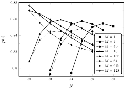
Figure 3: The achievable maximal single-photon probability $P^{(1)}$ at the optimal choice of the input mean photon number $\lambda_{\text{opt}}$ as a function of the number of multiplexed time windows $N$ on semi-logarithmic scale for various number of spatially multiplexed time multiplexers $M$. Loss parameters of the analyzed multiplexer are the following: $V_{r}=0.996$, $V_{t}=0.97$, $V_{p}=0.95$, $V_{p0,S}=0.996$, $V_{D}=0.9$, $V_{b}=1$. Points connected with continuous lines correspond to single-photon probabilities of combined multiplexers operating with the priority logic choosing the photon in the arm of the spatial multiplexer with the lowest loss and points with dotted lines to the one which simply routes the first arriving photon to the output.

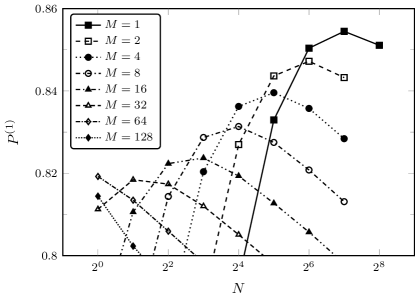
Figure 4: The achievable maximal single-photon probability $P^{(1)}$ at the optimal choice of the input mean photon number $\lambda_{\text{opt}}$ as a function of the number of multiplexed time windows $N$ on semi-logarithmic scale for various number of spatially multiplexed time multiplexers $M$. Loss parameters of the analyzed multiplexer are the following: $V_{r}=0.996$, $V_{t}=0.97$, $V_{p}=0.95$, $V_{p0,S}=0.985$, $V_{D}=0.9$, $V_{b}=1$.

Table 2: Maximal single-photon probabilities $P_{C,\max}^{(1)}$ of the combined multiplexers and the number of multiplexed time windows $N_{C,\text{opt}}$ and spatially multiplexed SPDC sources $M_{C,\text{opt}}$ at which they can be achieved for various loss parameter combinations. The maximal single photon probabilities $P_{T,\max}^{(1)}=P_{S,\max}^{(1)}=P_{T,S,\max}^{(1)}$ of the spatial and time multiplexers if optimized themselves are also presented. The first three rows show cases where combined multiplexing does not enhance the maximal single-photon probabilities of spatial and time multiplexers. The second and the last three rows present cases where combined multiplexing leads to a slightly higher and a definitely higher maximal single-photon probability, respectively.

No.	$V_{t}$	$V_{r}$	$V_{p}$	$V_{t,S}$	$V_{r,S}$	$V_{p0,S}$	$P_{T,S,\max}^{(1)}$	$M_{S,\rm opt}$	$N_{T,\rm opt}$	$P_{C,\max}^{(1)}$	$M_{C,\rm opt}$	$N_{C,\rm opt}$
1.	0.970	0.996	0.9500	0.970	0.996	0.9922	0.8545	128	128	0.8531	2	64
2.	0.988	0.991	0.9589	0.988	0.991	0.9950	0.8784	128	256	0.8784	2	128
3.	0.988	0.992	0.9568	0.990	0.991	0.9949	0.8812	128	256	0.8806	2	128
4.	0.988	0.990	0.9507	0.988	0.990	0.9940	0.8683	128	128	0.8684	2	64
5.	0.990	0.996	0.9297	0.986	0.993	0.9950	0.8834	128	256	0.8840	2	128
6.	0.990	0.996	0.9508	0.990	0.996	0.9943	0.8996	256	256	0.8999	2	128
7.	0.970	0.993	0.9606	0.980	0.993	0.9910	0.8506	128	128	0.8475	2	64
8.	0.980	0.993	0.9656	0.990	0.996	0.9901	0.8740	128	128	0.8720	2	64
9.	0.980	0.996	0.9655	0.990	0.992	0.9950	0.8860	128	256	0.8822	2	128
10.	0.980	0.990	0.9501	0.970	0.996	0.9917	0.8516	128	128	0.8541	2	64
11.	0.990	0.991	0.9493	0.980	0.995	0.9940	0.8762	128	256	0.8799	4	64
12.	0.990	0.993	0.9518	0.980	0.996	0.9951	0.8869	128	256	0.8906	4	64

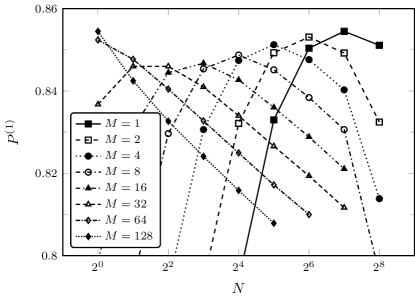
Figure 5: The achievable maximal single-photon probability $P^{(1)}$ at the optimal choice of the input mean photon number $\lambda_{\text{opt}}$ as a function of the number of multiplexed time windows $N$ on semi-logarithmic scale for various number of spatially multiplexed time multiplexers $M$. Loss parameters of the analyzed multiplexer are the following: $V_{r}=V_{r,S}=0.996$, $V_{t}=V_{t,S}=0.97$, $V_{p}=0.95$, $V_{p0,S}=0.9922$, $V_{D}=0.9$, $V_{b}=1$.

Figure 6: The achievable maximal single-photon probability $P^{(1)}$ at the optimal choice of the input mean photon number $\lambda_{\text{opt}}$ as a function of the number of multiplexed time windows $N$ on semi-logarithmic scale for various number of spatially multiplexed time multiplexers $M$. Loss parameters of the analyzed multiplexer are the following: $V_{r}=0.993$, $V_{r,S}=0.996$, $V_{t}=0.99$, $V_{t,S}=0.98$, $V_{p}=0.95$, $V_{p0,S}=0.995$, $V_{D}=0.9$, $V_{b}=1$.

Let us first analyze the case when the maximal single-photon probability of the spatial multiplexer is higher than that of the time multiplexer, that is, $P_{S,\max}^{(1)}>P_{T,\max}^{(1)}$. In Fig. 3 we show the achievable maximal single-photon probability $P^{(1)}$ at the optimal choice of the input mean photon number $\lambda_{\text{opt}}$ as a function of the number of multiplexed time windows $N$ for various number of spatially multiplexed time multiplexers $M$ for an experimentally feasible set of loss parameters. The high performance $P_{S,\max}^{(1)}=0.8763$ of the spatial multiplexer is ensured by choosing a transmission efficiency as high as $V_{p0,S}=0.996$. In this figure the curve $M=1$ corresponds to standalone time multiplexers while the points at $N=2^{0}=1$ are calculated for standalone spatial multiplexers. The figure shows results for both of the considered priority logics treated in Sec. III. The points connected with dotted lines correspond to the logic which routes the signal photons from the first detected heralding event to the output. The points connected with continuous lines correspond to the improved logic choosing the spatial arm of the lowest loss. For $M=1$ (no spatial multiplexing) or $N=1$ (no time multiplexing) obviously the two logics produce the same performance. For the other choices of $N$ and $M$, combined multiplexers operating with the priority logic choosing the photon in the arm of the spatial multiplexer with the lowest loss produce always higher single-photon probabilities. Let us note here that we have made this comparison for all the following calculations, and we have found that the improved logic always outperforms the simpler one. Therefore, while we emphasize this fact here, we omit the details of this comparison in what follows.

The absolute maximal single-photon probability in Fig. 3 is at $M=128$ and $N=1$. This suggests that the best choice would be not to apply time multiplexing at all. However, the corresponding spatial multiplexer would involve 128 SPDC sources in the considered bulk optics setup, which is clearly unreasonable in practice. Combined multiplexing, on the other hand, can solve the issue of system size: single-photon probabilities over 86% can be achieved, for instance, with just 4 SPDC sources. Thus in this case, combined multiplexing enhances the achievable maximal single-photon probability $P^{(1)}=85.4\%$ of a single bulk time multiplexer. Notice that single-photon probabilities over 86% can be achieved with less than $N=128$ multiplexed time windows. As a consequence of this decrease of the number of time windows, higher repetition rates can be achieved with combined multiplexers, as compared to optimized single time multiplexers.

Moreover, the described advantage of the combined multiplexing is valid for several configurations with different number of spatially multiplexed sources $M$ and multiplexed time windows $N$. For such points the single-photon probability of the combined system is between the maximal probabilities of the standalone spatial and time multiplexers but the values of $M$ and $N$ in the combined system are smaller than the values $M_{S,\text{opt}}$ and $N_{T,\text{opt}}$ in the optimized standalone systems. In addition, the single-photon probabilities are significantly higher than the ones that can be achieved with the suboptimal use of the standalone spatial multiplexer when the number of multiplexed units $M$ is far below the optimized value $M_{S,\text{opt}}$, that is, $M\leq M_{S,\text{opt}}/4$.

Now let us consider the complementary case when the maximal single-photon probability of the spatial multiplexer is lower than that of the time multiplexer, that is, $P_{S,\max}^{(1)}<P_{T,\max}^{(1)}$. In Fig. 4 the achievable maximal single-photon probability $P^{(1)}$ is plotted at the optimal choice of the input mean photon number $\lambda_{\text{opt}}$ as a function of the number of multiplexed time windows $N$, for various numbers of spatially multiplexed time multiplexers $M$, for an experimentally feasible set of loss parameters. In this case the propagational transmission efficiency of the spatial multiplexer is chosen to be $V_{p0,S}=0.985$, and it has maximal single-photon probability $P_{S,\max}^{(1)}=82\%$ at $M=64$. It appears that combined multiplexing does not enhance the absolute maximum of single-photon probability ($P_{T,\max}^{(1)}=85.4\%$ at $M=1$, $N=128$) at all in this case. On the other hand, when the number of time windows $N$ is far below the optimized value $N_{T,\text{opt}}$, that is, $N\leq N_{T,\text{opt}}/4$, there are lots of combinations of $M$ and $N$ for which the single-photon probability is higher than one can achieve by this suboptimal use of a standalone time multiplexer. Therefore the benefit of the application of the spatial multiplexer is the possible enhancement of the repetition rate as described before, without the relevant decrease of the single-photon probabilities.

We have analyzed the two cases described above for a variety of different sets of loss efficiencies. Without going into details we remark here that we found the described behavior for all of the choices.

Finally, let us analyze the third possibility when the maximal single-photon probabilities of the spatial and time multiplexers, provided that they are optimized themselves, are equal within a given precision, that is, $P_{S,\max}^{(1)}=P_{T,\max}^{(1)}=P_{T,S,\max}^{(1)}$. We have performed simulations for several combinations of the loss parameters ensuring this equality. We have found that the maximal single-photon probability $P_{C,\max}^{(1)}$ of the combined system can be slightly lower or higher than the maximal single-photon probability $P_{T,S,\max}^{(1)}$ of the spatial and time multiplexers. The difference is generally so small that it cannot be detected in an experiment. As a consequence these quantities can be considered as roughly equal. For certain parameter sets these probabilities are really equal at the given precision. Beside this behavior we have found some rather special sets of loss parameters for which the single-photon probability of the combined system is definitely, yet not significantly lower or higher than that of the spatial or time multiplexed systems separately. Table 2 shows some examples for all these behaviors. In this table we present the maximal single-photon probabilities $P_{C,\max}^{(1)}$ of the combined multiplexers and the number of multiplexed time windows $N_{\text{opt}}$ and spatially multiplexed SPDC sources $M_{\text{opt}}$ at which they can be achieved for various loss parameter combinations. The maximal single photon probabilities $P_{T,S,\max}^{(1)}$ of the spatial and time multiplexers if optimized themselves are also presented.

Rows 1-6 of Tab. 2 contain cases when the optimized performance of the combined multiplexer is roughly equal to that of the standalone spatial and time multiplexers. The first three rows show examples for parameters for which the single-photon probability of the combined multiplexer $P_{C,\max}^{(1)}$ is slightly lower, while for the parameters in the second three rows it is slightly higher than that of the standalone multiplexers $P_{T,S,\max}^{(1)}$. We note that for the parameter set presented in row 2 all the single-photon probabilities are equal at the given precision, although the previous statement is true for this example. Rows 7-9 of Tab. 2 show examples for parameters for which the single-photon probability of the combined multiplexer $P_{C,\max}^{(1)}$ is definitely lower, while for the parameters in the last three rows it is definitely higher than that of the standalone multiplexers $P_{T,S,\max}^{(1)}$. The difference in the probabilities exceeds 0.002 (0.2%). Such a behavior occurs only if at least one of the transmission and reflection efficiencies of the applied PBS-s differs for the time and spatial multiplexers. An interesting feature that can be deduced from Tab. 2 is that the product of the optimal number of spatially multiplexed time multiplexers $M_{C,\rm opt}$ and the optimal number of multiplexed time windows $N_{C,\rm opt}$ for the combined system is equal to the optimal number of multiplexed time windows $N_{T,\rm opt}$ for the standalone time multiplexed source, that is, $M_{C,\rm opt}N_{C,\rm opt}=N_{T,\rm opt}$. This property is valid for other combined configurations, presented in Figs. 3-6, for certain sets of the number of spatially multiplexed time multiplexers $M$ and the number of time windows $N$ ensuring the best performance of the given combined multiplexed system. In these figures, such values of $M$ are $M\leq 32,16,16$ and $32$, respectively. Table 2 also shows, taking into account previous considerations as well, that by using combined multiplexing systems realized in bulk optics single-photon probabilities between 85% and 89% can be achieved experimentally.

Figs. 5 and 6 show the achievable maximal single-photon probability $P^{(1)}$ at the optimal choice of the input mean photon number $\lambda_{\text{opt}}$ as a function of the number of multiplexed time windows $N$ for various numbers of spatially multiplexed time multiplexers $M$ for the loss parameters presented in the first and the last rows of Tab. 2, respectively. In Fig. 6 one can see that beside the point corresponding to the maximal single-photon probability ($M_{C,\text{opt}}=4$ and $N_{C,\text{opt}}=64$) there are other $(M,N)$ pairs for this configuration [(2,64), (2,128), (2,256), (4,32), (4,128), (8,32), (8,64)] at which the single-photon probability exceeds the maximal single-photon probabilities of the standalone spatial and time multiplexers. These figures also show that there are several choices of $M$ and $N$ for which the single-photon probabilities are higher than one can achieve by suboptimal use of a standalone spatial or time multiplexer. Furthermore, these are not significantly lower than the maximal value. The aforementioned benefits of the combined approach, namely the decrease of the required SPDC sources and improvement of the achievable repetition rate, are also present in these cases. Finally, as we have already mentioned before, combined multiplexing allows continuous pumping of the system, which appears as an additional advantage of this arrangement.

V Conclusions

We have studied periodic single-photon sources based on combined multiplexing, in which the outputs of several time multiplexers are spatially multiplexed. We have set up a general framework for the description and optimization of such devices. Such systems can be realized most efficiently in bulk optics. We have pointed out that due to the asymmetry present in such a setup, it is possible to design an improved priority logic for the spatial part of the multiplexer.

We have shown that combined multiplexing systems can be optimized in order to achieve maximal single-photon probability for various sets of loss parameters by the appropriate choice of the number of spatially multiplexed time multiplexers, the number of multiplexed time windows and the input mean photon number.

According to our results concerning bulk optical combined multiplexers, if either the spatial or the time multiplexer outperforms the other, the combination can achieve an improvement compared to the worse one, even though it cannot be superior to the absolute maximum defined by the better one. If the spatial and time multiplexers themselves have a similar optimum performance, their combination may yield an enhanced single-photon probability in some special cases.

Finally, let us note that the performance of the combined multiplexers is generally higher than that of the standalone time or spatial multiplexers below optimized system size. More importantly, the combination can lead to a decrease in the number of the required SPDC sources or a possible increase of the achievable repetition rate of the system compared to the standalone use of the optimized spatial or time multiplexers, while still maintaining a relatively high single-photon probability. All these features of combined multiplexing can be essential from the point of view of experiments.

- (1) E. Knill, R. Laflamme, and G. J. Milburn, Nature 409, 46 (2001).
- (2) P. Kok, W. J. Munro, K. Nemoto, T. C. Ralph, J. P. Dowling, and G. J. Milburn, Rev. Mod. Phys. 79, 135 (2007).
- (3) N. Gisin, G. Ribordy, W. Tittel, and H. Zbinden, Rev. Mod. Phys. 74, 145 (2002).
- (4) V. Scarani, H. Bechmann-Pasquinucci, N. J. Cerf, M. Dušek, N. Lütkenhaus, and M. Peev, Rev. Mod. Phys. 81, 1301 (2009).
- (5) L.-M. Duan, M. D. Lukin, J. I. Cirac, and P. Zoller, Nature 414, 413 (2001).
- (6) N. Sangouard, C. Simon, H. de Riedmatten, and N. Gisin, Rev. Mod. Phys. 83, 33 (2011).
- (7) C. H. Bennett, G. Brassard, C. Crépeau, R. Jozsa, A. Peres, and W. K. Wootters, Phys. Rev. Lett. 70, 1895 (1993).
- (8) D. Bouwmeester, J.-W. Pan, K. Mattle, M. Eibl, H. Weinfurter, and A. Zeilinger, Nature 390, 575 (1997).
- (9) Z. Merali, Science 331, 1380 (2011).
- (10) M. Koniorczyk, L. Szabó, and P. Adam, Phys. Rev. A 84, 044102 (2011).
- (11) J. B. Spring, B. J. Metcalf, P. C. Humphreys, W. S. Kolthammer, X.-M. Jin, M. Barbieri, A. Datta, N. Thomas-Peter, N. K. Langford, D. Kundys, J. C. Gates, B. J. Smith, P. G. R. Smith, and I. A. Walmsley, Science 339, 798 (2013).
- (12) M. A. Broome, A. Fedrizzi, S. Rahimi-Keshari, J. Dove, S. Aaronson, T. C. Ralph, and A. G. White, Science 339, 794 (2013).
- (13) M. Tillmann, B. Dakic, R. Heilmann, S. Nolte, A. Szameit, and P. Walther, Nature Photon. 7, 540 (2013).
- (14) C. C. Gerry, Phys. Rev. A 59, 4095 (1999).
- (15) A. P. Lund, H. Jeong, T. C. Ralph, and M. S. Kim, Phys. Rev. A 70, 020101 (2004).
- (16) B. He, M. Nadeem, and J. A. Bergou, Phys. Rev. A 79, 035802 (2009).
- (17) P. Adam, T. Kiss, Z. Darázs, and I. Jex, Phys. Scripta 2010, 014011 (2010).
- (18) C.-W. Lee, J. Lee, H. Nha, and H. Jeong, Phys. Rev. A 85, 063815 (2012).
- (19) M. Hijlkema, B. Weber, H. P. Specht, S. C. Webster, A. Kuhn, and G. Rempe, Nature Phys. 3, 253-255 (2007).
- (20) J. McKeever, A. Boca, A. D. Boozer, R. Miller, J. R. Buck, A. Kuzmich, and H. J. Kimble, Science 303, 1992 (2004).
- (21) H. G. Barros, A. Stute, T. E. Northup, C. Russo, P. O. Schmidt, and R. Blatt, New J. Phys. 11, 103004 (2009).
- (22) M. Keller, B. Lange, K. Hayasaka, W. Lange, and H. Walther, Nature 431, 1075 (2004).
- (23) B. Lounis and W. E. Moerner, Nature 407, 491 (2000).
- (24) R. Lettow, Y. L. A. Rezus, A. Renn, G. Zumofen, E. Ikonen, S. Götzinger, and V. Sandoghdar, Phys. Rev. Lett. 104, 123605 (2010).
- (25) A. Beveratos, R. Brouri, T. Gacoin, A. Villing, J.-P. Poizat, and P. Grangier, Phys. Rev. Lett. 89, 187901 (2002).
- (26) T. Gaebel, I. Popa, A. Gruber, M. Domhan, F. Jelezko, and J. Wrachtrup, New J. Phys. 6, 98 (2004).
- (27) E. Wu, J. R. Rabeau, G. Roger, F. Treussart, H. Zeng, P. Grangier, S. Prawer, and J.-F. Roch, New J. Phys. 9, 434 (2007).
- (28) C. Santori, D. Fattal, J. Vuckovic, G. S. Solomon, and Y. Yamamoto, Nature 419, 594 (2002).
- (29) S. Strauf, N. G. Stoltz, M. T. Rakher, L. A. Coldren, P. M. Petroff, and D. Bouwmeester, Nature Photon. 1, 704 (2007).
- (30) S. V. Polyakov, A. Muller, E. B. Flagg, A. Ling, N. Borjemscaia, E. Van Keuren, A. Migdall, and G. S. Solomon, Phys. Rev. Lett. 107, 157402 (2011).
- (31) B. J. Smith, P. Mahou, O. Cohen, J. S. Lundeen, and I. A. Walmsley, Opt. Express 17, 23589 (2009).
- (32) O. Cohen, J. S. Lundeen, B. J. Smith, G. Puentes, P. J. Mosley, and I. A. Walmsley, Phys. Rev. Lett. 102, 123603 (2009).
- (33) C. Söller, O. Cohen, B. J. Smith, I. A. Walmsley, and C. Silberhorn, Phys. Rev. A 83, 031806(R) (2011).
- (34) P. J. Mosley, J. S. Lundeen, B. J. Smith, P. Wasylczyk, A. B. U’Ren, C. Silberhorn, and I. A. Walmsley, Phys. Rev. Lett. 100, 133601 (2008).
- (35) P. G. Evans, R. S. Bennink, W. P. Grice, T. S. Humble, and J. Schaake, Phys. Rev. Lett. 105, 253601 (2010).
- (36) T. Zhong, F. N. C. Wong, T. D. Roberts, and P. Battle, Opt. Express 17, 12019 (2009).
- (37) G. Brida, I. P. Degiovanni, M. Genovese, A. Migdall, F. Piacentini, S. V. Polyakov, and I. R. Berchera, Opt. Express 19, 1484 (2011).
- (38) M. A. Broome, M. P. Almeida, A. Fedrizzi, and A. G. White, Opt. Express 19, 22698 (2011).
- (39) M. Fiorentino, S. M. Spillane, R. G. Beausoleil, T. D. Roberts, P. Battle, and M. W. Munro, Opt. Express 15, 7479 (2007).
- (40) A. Eckstein, A. Christ, P. J. Mosley, and C. Silberhorn, Phys. Rev. Lett. 106, 013603 (2011).
- (41) M. Förtsch, J. U. Fürst, C. Wittmann, D. Strekalov, A. Aiello, M. V. Chekhova, C. Silberhorn, G. Leuchs, and C. Marquardt, Nat. Commun. 4, 1818 (2013).
- (42) A. L. Migdall, D. Branning, and S. Castelletto, Phys. Rev. A 66, 053805 (2002).
- (43) J. H. Shapiro and F. N. Wong, Opt. Lett. 32 , 2698 (2007).
- (44) X.-s. Ma, S. Zotter, J. Kofler, T. Jennewein, and A. Zeilinger, Phys. Rev. A 83, 043814 (2011).
- (45) M. Collins, C. Xiong, I. Rey, T. Vo, J. He, S. Shahnia, C. Reardon, T. Krauss, M. Steel, A. Clark, and B. Eggleton, Nat. Commun. 4, 2582 (2013).
- (46) T. Meany, L. A. Ngah, M. J. Collins, A. S. Clark, R. J. Williams, B. J. Eggleton, M. J. Steel, M. J. Withford, O. Alibart, and S. Tanzilli, Laser Photon. Rev. 8: L42-L46, (2014).
- (47) C. Xiong, M. J. Collins, M. J. Steel, T.F. Krauss, B. J. Eggleton, and A. S. Clark, IEEE J. Sel. Top. Quantum Electron. 21, 6400510 (2015).
- (48) T. B. Pittman, B. C. Jacobs, and J. D. Franson, Phys. Rev. A 66, 042303 (2002).
- (49) E. Jeffrey, N. A. Peters, and P. G. Kwiat, New J. Phys. 6, 100 (2004).
- (50) P. P. Rohde, L. G. Helt, M. J. Steel, and A. Gilchrist, Phys. Rev. A 92, 053829 (2015).
- (51) F. Kaneda, B. G. Christensen, J. J. Wong, H. S. Park, K. T. McCusker, and P. G. Kwiat, Optica 2, 1010 (2015).
- (52) R. J. A. Francis-Jones and P. J. Mosley, arXiv: 1503.06178.
- (53) C. T. Schmiegelow and M. A. Larotonda, Appl. Phys. B 116, 447 (2014).
- (54) J. Mower and D. Englund, Phys. Rev. A 84, 052326 (2011).
- (55) P. Adam, M. Mechler, I. Santa, and M. Koniorczyk, Phys. Rev. A 90, 053834 (2014).
- (56) D. Bonneau, G. J. Mendoza, J. L. O’Brien, and M. G. Thompson, New J. Phys. 17, 043057 (2015).
- (57) B. L. Glebov, J. Fan, and A. Migdall, Appl. Phys. Lett. 103, 031115 (2013).
- (58) G. J. Mendoza, R. Santagati, J. Munns, E. Hemsley, M. Piekarek, E. Martín-López, G. D. Marshall, D. Bonneau, M. G. Thompson, and J. L. O’Brien, Optica 3, 127 (2016)
- (59) I. Z. Latypov, A. V. Shkalikov, and A. A. Kalachev, J. Phys. Conf. Ser. 613, 012009 (2015).
- (60) L. Mazzarella, F. Ticozzi, A. V. Sergienko, G. Vallone, and P. Villoresi, Phys. Rev. A 88, 023848 (2013).
- (61) Rong-Chung Tyan, Atul A. Salvekar, Hou-Pu Chou, Chuan-Cheng Cheng, Axel Scherer, Pang-Chen Sun, Fang Xu, and Yeshayahu Fainman, J. Opt. Soc. Am. A 14, 1627-1636 (1997).
- (62) S. Kim, G. P. Nordin, J. Cai, and J. Jiang, Opt. Lett. 28, 2384-2386 (2003).
- (63) S. Virally, S. Lacroix, and N. Godbout, Phys. Rev. A 81, 013808 (2010).
- (64) A. Christ and C. Silberhorn, Phys. Rev. A 85, 023829 (2012).