Exponential ergodicity for a class of non-Markovian stochastic processes

Abstract.

We prove the convergence at an exponential rate towards the invariant probability measure for a class of solutions of stochastic differential equations with finite delay. This is done, in this non-Markovian setting, using the cluster expansion method, inspired from [4] or [14]. As a consequence, the results hold for small perturbations of ergodic diffusions.

Introduction

The aim of this paper is to prove the exponential ergodicity towards the unique invariant probability measure for some solutions of stochastic differential equations with finite delay and non regular drift.

We will consider $\displaystyle\mathbb{R}^{d}$-valued stochastic differential equations of the form :

$$dx_{t}=\left(g(x_{t})+\sigma\;b((x)_{t-t_{0}}^{t})\right)dt+\sigma\;dB_{t}$$

for a small additional drift term $\displaystyle b$, whose only requirement is to be measurable and bounded, and with certain assumptions on the underlying semi-group of the reference process solution of

$$dy_{t}=g(y_{t})dt+\sigma\;dB_{t}$$

Such an interest in those equations comes from a desire to obtain similar results for stochastic Cucker-Smale type models (such as the one presented by Ha, Lee and Levy in [6]), which should be included in a future work.

While results about the existence of invariant probability measures for stochastic differential equations with delay can be found in the literature, going back to the 1964 paper of Itô and Nisio [8] (see [9] for a survey on the topic published in 2003 by Ivanov, Kazmerchuk and Swishchuk), they are mainly valid under strong regularity assumptions on the coefficients. Furthermore, very little has been told about exponential ergodicity for such processes.

As we are dealing with non-Markovian processes, most standard methods are not available to us. Our main tool here will be the so-called cluster expansion method, mainly used in statistical mechanics, in particular in Gibbs field theory. As a consequence, our results will hold for irregular but small (albeit not insignificant) perturbations of the reference process.

Technical results for the adaptation of the cluster expansion methods to Gibbs random fields can be found in the book [13] by Malyshev and Minlos. Subsequent papers have implemented those methods for stochastic processes, for example, interacting diffusions systems or one-dimensional non-Markovian diffusions. It was done by Ignatyuk, Malyshev and Sidoravicius in [7], and, more recently, amongst others in [4], [5] or [14].

Our main result, the exponential convergence of the semi-group towards the invariant probability measure, implies that the decay of correlations is exponentially quick, i.e. we have what is called exponential decorrelation : there exist two constants $\displaystyle\theta_{1}$ and $\displaystyle\theta_{2}$ such that for all $\displaystyle f$ and $\displaystyle g$ measurable and bounded by $\displaystyle 1$, it holds :

$$|cov(f(x_{t}),g(x_{t+s}))|\leqslant\theta_{1}\;e^{-\theta_{2}s}$$

It follows that a central limit theorem can be derived from the mixing properties implied by this inequality.

Contrary to what was done in [4], we do not require for the semi-group associated with the process to be ultracontractive, but only need some strong form of hypercontractivity. One instance of a well-known process which is not ultracontractive but verifies our assumptions is the Ornstein-Uhlenbeck process. We will present some explicit results in this particular setting. Actually, the stochastic Cucker-Smale model can be seen as a mean-field perturbation of the Ornstein-Uhlenbeck process, and this led to this work.

Under those less restrictive hypotheses, the lack of ultracontractive bounds for the underlying reference process introduces several new technical difficulties. We will therefore present a detailed proof for the obtaining of the cluster estimates. The use of these estimates to get to the final main theorem follows the lines of, for instance, [12] and will not be detailed here.

We start by introducing our framework, the objects we will manipulate and the assumptions that will be needed. Then, we set out to obtain a cluster representation for the partition function defined in the first part. In section 3, we study the cluster estimates and show that they tend to $\displaystyle 0$ when the norm of $\displaystyle b$ does. We present the main results in section 4. Finally, in section 5, we explicitly compute some of the bounds in the Ornstein-Uhlenbeck setting.

1. Framework and assumptions

Let $\displaystyle\Omega$ be the space of real $\displaystyle\mathbb{R}^{d}$-valued continuous functions for some $\displaystyle d\geqslant 1$.

1.1. A few notations

We set the following notations :

• $\displaystyle a$, a fixed positive number, destined to become quite large ;

• for every $\displaystyle j$ in $\displaystyle\mathbb{Z}$, $\displaystyle I_{j}=[ja,(j+1)a]$ ;

• for every $\displaystyle N$ in $\displaystyle\mathbb{N}^{*}$, $\displaystyle I(N)=[-Na,Na]=\bigcup_{j=-N}^{N-1}I_{j}$ ;

• for every $\displaystyle u$ in $\displaystyle\Omega$, $\displaystyle u^{(N)}(t)=u(Na)$ if $\displaystyle t\geqslant Na$, $\displaystyle u^{(N)}(t)=u(t)$ if $\displaystyle-Na\leqslant t\leqslant Na$, and $\displaystyle u^{(N)}(t)=u(-Na)$ if $\displaystyle t\leqslant-Na$. That is : $\displaystyle u^{(N)}$ is equal to $\displaystyle u$ frozen outside of the interval $\displaystyle I(N)$.

1.2. The stochastic processes under consideration : hypotheses (H1) and (H2)

We introduce here the process which will serve as a reference in our work : a stochastic process sufficiently regular to be exponentially ergodic towards its invariant probability measure. We present all the assumptions that will be necessary to extend this ergodicity to small perturbations of this process.

We consider the following stochastic differential equation :

(1) $$dy_{t}=g(y_{t})dt+\sigma\;dB_{t}$$

with $\displaystyle g:\mathbb{R}^{d}\rightarrow\mathbb{R}^{d}$ a smooth function, $\displaystyle\sigma$ an invertible $\displaystyle d\times d$ matrix, and $\displaystyle B$ a standard $\displaystyle d$-dimensional Brownian motion.

We assume that $\displaystyle(y_{t})_{t\in\mathbb{R}_{+}}$ is a $\displaystyle\mathbb{R}^{d}$-valued stochastic process, solution of (1) with initial condition $\displaystyle y_{0}=y^{0}$. For every $\displaystyle f$ regular enough, we define $\displaystyle P_{t}f$ its semi-group at time $\displaystyle t$, that is, for any given $\displaystyle x$, $\displaystyle P_{t}f(x)=\mathbb{E}_{x}[f(y_{t})]$, and its infinitesimal generator $\displaystyle L=\frac{1}{2}\sum_{i,j}a_{ij}\partial^{2}_{ij}+\sum_{i}g_{i}\partial i$, with $\displaystyle a_{ij}=(\sigma\sigma^{*})_{ij}$.

We will suppose that $\displaystyle(y_{t})$ admits a symmetric probability measure $\displaystyle\mu$, i.e. for all $\displaystyle f$ and $\displaystyle g$ smooth enough, $\displaystyle\int fLg\>d\mu=\int gLf\>d\mu$. Thus, $\displaystyle\mu$ is an invariant measure : for every $\displaystyle f$ smooth enough, $\displaystyle\mathbb{E}_{\mu}[f(y_{t})]=\int f\;d\mu$. Since there exists $\displaystyle\alpha>0$ such that for all $\displaystyle\xi\in\mathbb{R}^{d}$, $\displaystyle\xi^{*}\sigma\sigma^{*}\xi\geqslant\alpha|\xi|^{2}$, the generator is uniformly elliptic and it is well-known that $\displaystyle\mu$ is absolutely continuous with respect to Lebesgue measure with a positive density. Thus, $\displaystyle\mu$ is of the form $\displaystyle d\mu(x)=C\;e^{-V(x)}dx$ ; in addition, it is known that $\displaystyle V:\mathbb{R}^{d}\rightarrow\mathbb{R}$ is smooth.

According to Kolmogorov’s characterization of reversible diffusions, in [11], this even implies that $\displaystyle\mu$ is symmetric for the semi-group $\displaystyle(P_{t})_{t\geqslant 0}$ and that $\displaystyle g$ can be written as $\displaystyle g=-\frac{1}{2}\;\sigma\;\nabla V$. Thus, equation (1) becomes :

(2) $$dy_{t}=-\frac{1}{2}\;\sigma\;\nabla V(y_{t})dt+\sigma\;dB_{t}$$

Our assumptions imply that $\displaystyle(y_{t})$ is non-explosive and $\displaystyle(P_{t})$ admits a smooth transition density with respect to $\displaystyle\mu$, denoted by $\displaystyle p(t,x,y)$. As the process $\displaystyle(y_{t})_{t\geqslant 0}$ is reversible with respect to the stationary measure $\displaystyle\mu$,

$$\forall\;t,x,y,\quad p(t,x,y)=p(t,y,x).$$

We now introduce two hypotheses which will be essential in the following :

• (H1) : $\displaystyle\mu$ satisfies a Poincaré inequality : there exists a constant $\displaystyle C_{P}$ such that for all smooth functions $\displaystyle f$ in $\displaystyle\mathcal{L}^{2}(\mu)$,

  $$\|\;f-\int f\;d\mu\;\|^{2}_{\mathcal{L}^{2}(\mu)}\leqslant C_{P}\int|\sigma\;\nabla f|^{2}\;d\mu$$

• (H2) : There exists $\displaystyle\delta\geqslant 0$ such that

  $$\sup_{t\geqslant\delta}\|p(t,.,.)\|_{\mathcal{L}^{8}(\mu\otimes\mu)}<\infty$$

Remark 1.

Actually, we only require $\displaystyle\|p(t,.,.)\|_{\mathcal{L}^{8}(\mu\otimes\mu)}$ to be finite for certain values of $\displaystyle t$ and it is not necessary for the supremum over $\displaystyle t$ to be finite. However, the current form of (H2) simplifies the writing of the proofs, and it is satisfied by the important case of the Ornstein-Uhlenbeck process, as will be seen in section 5.

Remark 2.

Using Cauchy-Schwarz’s and Jensen’s inequalities,

$\displaystyle\begin{array}[]{lll}\|P_{\delta}f\|_{\mathcal{L}^{8}(\mu)}^{8}&=&\int\left(\int p(\delta,x,y)f(y)\;\mu(dy)\right)^{8}\mu(dx)\\ &\leqslant&\int\left(\int|f(y)|^{2}\;\mu(dy)\right)^{4}\left(\int p(\delta,x,y)^{2}\;\mu(dy)\right)^{4}\mu(dx)\\ &\leqslant&\|f\|_{\mathcal{L}^{2}(\mu)}^{8}\int\int p(\delta,x,y)^{8}\;\mu(dy)\mu(dx)\end{array}$

This means that :

(3) $$\|P_{\delta}f\|_{\mathcal{L}^{8}(\mu)}\leqslant\|p(\delta,.,.)\|_{\mathcal{L}^{8}(\mu\otimes\mu)}\;\|f\|_{\mathcal{L}^{2}(\mu)}.$$

Thus, if (H2) is satisfied, $\displaystyle P_{\delta}:\mathcal{L}^{2}(\mu)\rightarrow\mathcal{L}^{8}(\mu)$ is a bounded operator and $\displaystyle(P_{t})_{t}$ is hyperbounded, that is, it verifies a defective log-Sobolev inequality : there exists non-negative constants $\displaystyle C_{LS}$ and $\displaystyle\rho$ such that for all smooth functions $\displaystyle f$ in $\displaystyle\mathcal{L}^{2}(\mu)$,

$$\int f^{2}\ln(f^{2})\;d\mu-\int f^{2}\;d\mu\;\ln\;(\int f^{2}d\mu)\leqslant C_{LS}\int|\sigma\;\nabla f|^{2}\;d\mu+\rho\int f^{2}d\mu$$

If, in addition, (H1) is satisfied, the semi-group $\displaystyle(P_{t})_{t}$ is hypercontractive, i.e. for every $\displaystyle k\geqslant 2$, there exists $\displaystyle\delta_{k}$ such that for every $\displaystyle t\geqslant\delta_{k}$, $\displaystyle P_{t}:\mathbb{L}^{2}\rightarrow\mathbb{L}^{k}$ is bounded by $\displaystyle 1$. Equivalently, it means that $\displaystyle\mu$ verifies a tight log-Sobolev inequality : there exists a non-negative constant $\displaystyle\bar{C}_{LS}$ such that for all smooth functions $\displaystyle f$ in $\displaystyle\mathcal{L}^{2}(\mu)$,

$$\int f^{2}\ln(f^{2})\;d\mu-\int f^{2}\;d\mu\;\ln\;(\int f^{2}d\mu)\leqslant\bar{C}_{LS}\int|\sigma\;\nabla f|^{2}\;d\mu$$

Remark 3.

It is well-known (see [1] for example) that hypothesis (H1) is equivalent to the exponential convergence of the semi-group towards $\displaystyle\mu$ :

(H1b) : There exists a constant $\displaystyle C_{S}$ such that for all $\displaystyle f\in\mathcal{L}^{2}(\mu)$, for all $\displaystyle t\geqslant 0$,

$$\|\;P_{t}f-\int f\;d\mu\;\|_{\mathcal{L}^{2}(\mu)}\leqslant e^{-C_{S}t}\|\;f-\int f\;d\mu\;\|_{\mathcal{L}^{2}(\mu)}$$

and, moreover, $\displaystyle C_{S}=1/C_{P}$ (see [3] for a more general statement).

In particular, if (H1) holds and $\displaystyle\int fd\mu=0$, then, for every $\displaystyle t\geqslant 0$,

(4) $$\|P_{t}f\|_{\mathcal{L}^{2}(\mu)}\leqslant e^{-t/C_{P}}\|f\|_{\mathcal{L}^{2}(\mu)}$$

We now prove two lemmas, the second one, resulting in part from the first one, taking into account hypotheses (H1) and (H2) and yielding the assumption we will use in practice, rather than (H1) itself.

Lemma 1.

Suppose that (H1) holds true. Then for all smooth $\displaystyle f$ such that $\displaystyle\int fd\mu=0$,

$$\forall t\geqslant\delta,\quad\|P_{t}f\|_{\mathcal{L}^{8}(\mu)}\leqslant\|p(\delta,.,.)\|_{\mathcal{L}^{8}(\mu\otimes\mu)}\;e^{-(t-\delta)/C_{P}}\;\|f\|_{\mathcal{L}^{8}(\mu)}$$

Remark 4.

It is possible for both sides of the above inequality to be infinite.

Proof.

Let $\displaystyle t$ be a positive number with $\displaystyle t\geqslant\delta$ and $\displaystyle f$ a smooth function such that $\displaystyle\int fd\mu=0$.

For any $\displaystyle t\geqslant\delta$, thanks to the inequality (3) proven in remark 2,

$\displaystyle\begin{array}[]{lll}\|P_{t}f\|_{\mathcal{L}^{8}(\mu)}&=&\|P_{\delta}(P_{t-\delta}f)\|_{\mathcal{L}^{8}(\mu)}\\ &\leqslant&\|p(\delta,.,.)\|_{\mathcal{L}^{8}(\mu\otimes\mu)}\;\|P_{t-\delta}f\|_{\mathcal{L}^{2}(\mu)}\end{array}$

As (H1) is supposed to be satisfied, so is (4) ; hence the conclusion of this proof :

$\displaystyle\begin{array}[]{lll}\|P_{t}f\|_{\mathcal{L}^{8}(\mu)}&\leqslant&\|p(\delta,.,.)\|_{\mathcal{L}^{8}(\mu\otimes\mu)}\;e^{-(t-\delta)/C_{P}}\|f\|_{\mathcal{L}^{2}(\mu)}\\ &\leqslant&\|p(\delta,.,.)\|_{\mathcal{L}^{8}(\mu\otimes\mu)}\;e^{-(t-\delta)/C_{P}}\|f\|_{\mathcal{L}^{8}(\mu)}\end{array}$

∎

Lemma 2.

Under hypotheses (H1) and (H2), for $\displaystyle t\geqslant 2\delta$,

$$\|p(t,x,y)-1\|_{\mathcal{L}^{8}(\mu\otimes\mu)}\leqslant\beta_{\delta}(t)\left(\|p(\delta,.,.)\|_{\mathcal{L}^{8}(\mu\otimes\mu)}\vee 1\right)$$

where $\displaystyle\beta_{\delta}(t)=2M_{\delta}\;e^{-(t-2\delta)/C_{P}}$ with $\displaystyle M_{\delta}=\sup_{a\geqslant\delta}\|p(a,.,.)\|_{\mathcal{L}^{8}(\mu\otimes\mu)}\vee 1$

In particular, $\displaystyle\beta_{\delta}(t)$ goes to $\displaystyle 0$ exponentially fast when $\displaystyle t$ goes to infinity.

Proof.

We start by expressing $\displaystyle p(t,x,y)-1$ using the semi-group :

$\displaystyle\begin{array}[]{lll}p(t,x,y)-1&=&\int\left(p(t-\delta,x,z)p(\delta,z,y)-1\right)\mu(dz)\\ &=&P_{t-\delta}(p(\delta,.,y))(x)-1\\ &=&P_{t-\delta}(p(\delta,.,y)-1)(x)\end{array}$

Thus, applying lemma 1 for $\displaystyle f=p(\delta,.,y)-1$ at time $\displaystyle t-\delta$ ($\displaystyle\geqslant\delta$ as $\displaystyle t\geqslant 2\delta$),

$\displaystyle\begin{array}[]{lll}\int(p(t,x,y)-1)^{8}\mu(dx)&=&\int P^{8}_{t-\delta}(p(\delta,.,y)-1)(x)\;\mu(dx)\\ &\leqslant&\|p(\delta,.,.)\|_{\mathcal{L}^{8}(\mu\otimes\mu)}^{8}\;e^{-8(t-2\delta)/C_{P}}\|p(\delta,.,y)-1\|_{\mathcal{L}^{8}(\mu)}^{8}\\ &\leqslant&2^{8}\|p(\delta,.,.)\|_{\mathcal{L}^{8}(\mu\otimes\mu)}^{8}\;e^{-8(t-2\delta)/C_{P}}\left(\|p(\delta,.,y)\|^{8}_{\mathcal{L}^{8}(\mu)}\vee 1\right),\end{array}$

which leads to :

$$\int(p(t,x,y)-1)^{8}\mu(dx)\mu(dy)\leqslant 2^{8}\|p(\delta,.,.)\|_{\mathcal{L}^{8}(\mu\otimes\mu)}^{8}\;e^{-8(t-2\delta)/C_{P}}\left(\|p(\delta,.,.)\|^{8}_{\mathcal{L}^{8}(\mu\otimes\mu)}\vee 1\right)$$

Hypothesis (H2) ensures that $\displaystyle\|p(u,.,.)\|_{\mathcal{L}^{8}(\mu\otimes\mu)}$ is bounded uniformly in $\displaystyle u$ for $\displaystyle u\geqslant\delta$, hence the result. ∎

Remark 5.

As can be seen in the proof, $\displaystyle M_{\delta}$ is a priori not the optimal bound (although it can correspond with $\displaystyle\|p(\delta,.,.)\|_{\mathcal{L}^{8}(\mu\otimes\mu)}$ as will be seen in the Ornstein-Uhlenbeck example in section 5) but will be good enough for our needs (and will simplify later computations).

In what follows, $\displaystyle P$ will be the law, on $\displaystyle\Omega$, of the stationary solution of (2). It will be our reference measure.

1.3. The perturbed equation

Having established properties and assumptions needed for the reference process, we turn our attention to the stochastic differential equation with finite delay $\displaystyle t_{0}$ :

(5) $$dx_{t}=\left(-\frac{1}{2}\;\sigma\;\nabla V(x_{t})+\sigma\;b((x)_{t-t_{0}}^{t})\right)dt+\sigma\;dB_{t}$$

where $\displaystyle V$, $\displaystyle\sigma$ and $\displaystyle B$ are as previously defined and $\displaystyle b:\mathcal{C}^{0}([-t_{0},0],\mathbb{R}^{d})\rightarrow\mathbb{R}^{d}$ is a bounded measurable function.

Let $\displaystyle Q$ be the law of $\displaystyle x$. For given numbers $\displaystyle a$ and $\displaystyle b$, and for an interval $\displaystyle I$, $\displaystyle Q_{I}^{a,b}$ shall be the law of the stochastic bridge associated with $\displaystyle x$ such that $\displaystyle y(\inf I)=a$ and $\displaystyle y(\sup I)=b$.

Remark 6.

We only require $\displaystyle b$ to be bounded and measurable, without any further assumption on its regularity. This is one of the main advantages of our method.
We give here a few examples (that should be renormalized to be small enough to satisfy the hypotheses of our main result, Theorem 2) :

• we can consider $\displaystyle b$ of the form $\displaystyle b((u)_{t-t_{0}}^{t})=\int_{t-t_{0}}^{t}f(u_{t},u_{s})\;ds$ for any trajectory $\displaystyle u\in\Omega$ with $\displaystyle f$ bounded and measurable ; for instance, $\displaystyle f(x,y)=\text{sign}(x-y)$ or $\displaystyle f(x,y)=\mathds{1}_{y\in A}$ with $\displaystyle A$ a subset of $\displaystyle\mathbb{R}^{d}$ (thus obtaining an occupation time);

• we may wish to have a dependence in the past depending on a single time, of the form $\displaystyle b((u)_{t-t_{0}}^{t})=g(u_{t-t_{0}})$ for a certain function $\displaystyle g$ measurable and bounded, but not necessarily continuous ;

• staying with non continuous perturbation drifts, one can also consider a function with jumps, such as $\displaystyle b((u)_{t-t_{0}}^{t})=\mathds{1}_{(u)_{t-t_{0}}^{t}\in A}$ with $\displaystyle A$ a subset of $\displaystyle\mathcal{C}^{0}([-t_{0},0],\mathbb{R}^{d})$.
  

Using Girsanov theorem (taken for instance from [12]), we can show that the restriction to some finite time interval $\displaystyle I$ of the law of $\displaystyle x$ is absolutely continuous with respect to the restricted law of the reference process $\displaystyle y$, and that its density is of the form $\displaystyle\exp(-H_{I}(u))du$ where the associated Hamiltonian $\displaystyle H_{I}$ is defined by

(6) $$H_{I}(u)=-\int_{I}b((u)_{t-t_{0}}^{t})^{*}\;dB_{t}+\frac{1}{2}\int_{I}|b((u)_{t-t_{0}}^{t})|^{2}\;dt$$

for every trajectory $\displaystyle u$ in the space state $\displaystyle\Omega$. We will denote $\displaystyle H_{N}=H_{I(N)}$.

Our goal is to prove the convergence of the sequence of measures $\displaystyle(Q_{N})$, defined on $\displaystyle\Omega$ by

(7) $$Q_{N}(du)=\exp(-H_{N}(u^{(N)}))P(du)$$

towards a weak solution of the equation (5) that will be time stationary. From this point, classical results of Gibbs theory shall provide further results, such as the exponential decorrelation.

To this end, we introduce the partition function $\displaystyle Z_{N}$ given by

(8) $$Z_{N}=\mathbb{E}_{\mu}[\exp(-H_{N})]$$

with $\displaystyle\mathbb{P}_{\mu}$ being the law under $\displaystyle\mu$ and $\displaystyle\mathbb{E}_{\mu}$ the associated expectation.

The aim of our next section will be to write $\displaystyle Z_{N}$ under the form of a cluster expansion. What this means shall be detailed next.

2. The cluster representation of the partition function

In this paragraph, we aim to expand the partition function into a “cluster expansion”, that is to obtain an expression of $\displaystyle Z_{N}$ of the form :

$$Z_{N}=1+\sum_{\tau}\prod_{i}\Gamma_{\tau_{i}}$$

with the meaning and nature of each of $\displaystyle\tau$, $\displaystyle i$ and $\displaystyle\Gamma_{\tau_{i}}$ to be determined.

A usual, we write $\displaystyle P(X=\;.\;|X^{\prime}=Z)$ for the conditional distribution of $\displaystyle X$ given $\displaystyle X^{\prime}=Z$, i.e. a regular desintegration of the $\displaystyle P$-law of $\displaystyle(X,X^{\prime})$ with respect to the law of $\displaystyle X^{\prime}$.

We start by conditioning with respect to the values taken at times $\displaystyle-Na$, …, $\displaystyle Na$ by the process $\displaystyle(y_{t})_{t}$:

$\displaystyle\begin{array}[]{lll}Z_{N}&=&\int_{\Omega}\exp(-H_{N}(u^{(N)}))P(du)\\ &=&\int_{\mathbb{R}^{(2N+1)d}}\int_{\Omega}\exp(-H_{N}(u^{(N)}))P(du|u(ja)=y_{j},j=-N,...,N)\\ &&\quad\quad\quad\quad\quad\quad\quad\quad\bigotimes_{j=-N}^{N-1}P(y((j+1)a)=dy_{j+1}|y(ja)=y_{j})\otimes P(y(-Na)=dy_{-N})\\ \end{array}$

Thus, first using the Markov property of $\displaystyle y$ and the definition of the bridges $\displaystyle Q_{I}^{a,b}$, and, second, introducing the transition densities $\displaystyle p(t,.,.)$ of $\displaystyle(y_{t})_{t}$ with respect to $\displaystyle\mu$,

$\displaystyle\begin{array}[]{lll}Z_{N}&=&\int_{\mathbb{R}^{(2N+1)d}}\int_{\Omega}\exp(-H_{N}(u^{(N)})\bigotimes_{j=-N}^{N-1}Q_{I_{j}}^{y_{j},y_{j+1}}(du)\left(\bigotimes_{j=-N}^{N-1}P(y(a)=dy_{j+1}|y(0)=y_{j})\right)\otimes\mu(dy_{-N})\\ &=&\int_{\mathbb{R}^{(2N+1)d}}\int_{\Omega}\exp(-H_{N}(u^{(N)}))\bigotimes_{j=-N}^{N-1}Q_{I_{j}}^{y_{j},y_{j+1}}(du)\left(\bigotimes_{j=-N}^{N-1}p(a,y_{j},y_{j+1})\mu(dy_{j+1})\right)\otimes\mu(dy_{-N})\\ \end{array}$

Next, we re-arrange the terms in a convenient way :

$$Z_{N}=\int_{\mathbb{R}^{(2N+1)d}}\int_{\Omega}\prod_{j=-N}^{N-1}\exp(-H_{I_{j}}(u^{(N)}))p(a,y_{j},y_{j+1})\bigotimes_{j=-N}^{N-1}Q_{I_{j}}^{y_{j},y_{j+1}}(du)\bigotimes_{j=-N}^{N}\mu(dy_{j})$$

Contrary to what was done, by mistake, between equations (13) and (14) in [4], we cannot exchange the product and the integral over $\displaystyle\Omega$. This can be corrected in a way by a different decomposition : we write :

(9) $$Z_{N}=\int_{\mathbb{R}^{(2N+1)d}}\int_{\Omega}\prod_{j=-N}^{N-1}\alpha_{j}(a,y,u)\bigotimes_{j=-N}^{N-1}Q_{I_{j}}^{y_{j},y_{j+1}}(du)\bigotimes_{j=-N}^{N}\mu(dy_{j})$$

$\displaystyle\begin{array}[]{llll}\text{ where }\alpha_{j}(a,y,u)&=&\exp(-H_{I_{-N}}(u^{(N)}))\sqrt{p(a,y_{-N},y_{-N+1})}&\text{if }j=-N\\ &=&\exp(-H_{I_{j}}(u^{(N)}))\sqrt{p(a,y_{j-1},y_{j})p(a,y_{j},y_{j+1})}&\text{if }j\in\{-N+1,...,N-2\}\\ &=&\exp(-H_{I_{N-1}}(u^{(N)}))\sqrt{p(a,y_{N-2},y_{N-1})}p(a,y_{N-1},y_{N})&\text{if }j=N-1\end{array}$

In order to obtain a sum of a product of terms that are “temporally independent” from each other, we rewrite differently the product of the $\displaystyle\alpha_{j}$ :

$\displaystyle\begin{array}[]{lll}\prod_{j=-N}^{N-1}\alpha_{j}(a,y,u)&=&\prod_{j=-N}^{N-1}(1+\alpha_{j}(a,y,u)-1)\\ &=&1+\sum_{S}\prod_{j\in S}(\alpha_{j}(a,y,u)-1)\end{array}$

where the sum is taken on all non-empty subsets $\displaystyle S$ of $\displaystyle\{-N,...N-1\}$.

Thus,

$$\prod_{j=-N}^{N-1}\alpha_{j}(a,y,u)=1+\sum_{p\in\mathbb{N^{*}}}\sum_{\;\tau_{1}\sqcup...\sqcup\tau_{p}}\;\prod_{i=1}^{p}\;\prod_{j\in\tau_{i}}\;(\alpha_{j}(a,y,u)-1)$$

with $\displaystyle\tau_{i}$ of the form $\displaystyle\{b,b+1,...,b+r\}$, $\displaystyle b,b+r\in I(N)$, and $\displaystyle d(\tau_{i},\tau_{j})\geqslant 2$

Coming back to the expression of the partition function,

$\displaystyle\begin{array}[]{lll}Z_{N}&=&\int_{\mathbb{R}^{(2N+1)d}}\int_{\Omega}\left(1+\sum_{p\in\mathbb{N^{*}}}\sum_{\;\tau_{1}\sqcup...\sqcup\tau_{p}\subset I(N)}\;\prod_{i=1}^{p}\;\prod_{j\in\tau_{i}}\;(\alpha_{j}(a,y,u)-1)\right)\bigotimes_{j=-N}^{N-1}Q_{I_{j}}^{y_{j},y_{j+1}}(du)\bigotimes_{j=-N}^{N}\mu(dy_{j})\\ &=&1+\sum_{p\in\mathbb{N^{*}}}\sum_{\;\tau_{1}\sqcup...\sqcup\tau_{p}\subset I(N)}\int_{\mathbb{R}^{(2N+1)d}}\int_{\Omega}\prod_{i=1}^{p}\;\prod_{j\in\tau_{i}}\;(\alpha_{j}(a,y,u)-1)\bigotimes_{j=-N}^{N-1}Q_{I_{j}}^{y_{j},y_{j+1}}(du)\bigotimes_{j=-N}^{N}\mu(dy_{j})\end{array}$

The decomposition of the product of the $\displaystyle\alpha_{j}$ was done with in mind the idea of inverting the product for $\displaystyle i$ from $\displaystyle 1$ to $\displaystyle p$ and both integrals. This is indeed now possible :

• Notice that $\displaystyle j_{1}\in\tau_{i_{1}}$ and $\displaystyle j_{2}\in\tau_{i_{2}}$ implies that $\displaystyle|j_{1}-j_{2}|\geqslant 2$.

  Take $\displaystyle\tau_{i}=\{b_{i},...,b_{i}+r_{i}\}$.
  

  As $\displaystyle\prod_{j\in\tau_{i}}\;(\alpha_{j}(a,y,u)-1)$ only depends on $\displaystyle u(t)$ for

  $$t\in\bigcup_{j\in\tau_{i}}[ja-t_{0},(j+1)a]=[(b_{i}a-t_{0}))\wedge(-Na),(b_{i}+r_{i}+1)a]\subset I_{b_{i}-1}\cup...\cup I_{b_{i}+r_{i}}$$

  and $\displaystyle(b_{i_{1}}+r_{i_{1}}+1)a<b_{i_{2}}a-t_{0}$ for $\displaystyle i_{1},i_{2}\in\{1,...,p\}$, $\displaystyle i_{1}\neq i_{2}$ and $\displaystyle a$ large enough, we have

  $$\left(I_{b_{i_{1}}-1}\cup...\cup I_{b_{i_{1}}+r_{i_{1}}}\right)\bigcap\left(I_{b_{i_{2}}-1}\cup...\cup I_{b_{i_{2}}+r_{i_{2}}}\right)=\emptyset.$$

  This allows us to invert the product of the $\displaystyle\alpha_{j}$ with the integral over $\displaystyle\Omega$ : we thus have

  $$Z_{N}=1+\sum_{p\in\mathbb{N^{*}}}\sum_{\;\tau_{1}\sqcup...\sqcup\tau_{p}}\int_{\mathbb{R}^{(2N+1)d}}\prod_{i=1}^{p}\left[\int_{\Omega}\prod_{j\in\tau_{i}}\;(\alpha_{j}(a,y,u)-1)\bigotimes_{k=b_{i}-1}^{b_{i}+r_{i}-1}Q_{I_{k}}^{y_{k},y_{k+1}}(du)\right]\bigotimes_{j=-N}^{N}\mu(dy_{j})$$

• Moreover, notice that the expression between the square brackets only depends on $\displaystyle y_{b_{i}-1},y_{b_{i}},...,y_{b_{i}+r_{i}}$. As a consequence, we can interchange the integral over $\displaystyle\mathbb{R}^{2N+1}$ and the product in $\displaystyle i$.

Thus, we obtain the following cluster representation of the partition function $\displaystyle Z_{N}$ :

(10) $$Z_{N}=1+\sum_{p\in\mathbb{N^{*}}}\sum_{\;\tau_{1}\sqcup...\sqcup\tau_{p}\subset I(N)}\;\prod_{i=1}^{p}\;\Gamma_{\tau_{i}}$$

where

(11) $$\Gamma_{\tau}=\int_{\mathbb{R}^{(|\tau|+1)d}}\int_{\Omega}\prod_{j\in\tau}\;(\alpha_{j}(a,y,u)-1)\bigotimes_{k=\min(\tau)-1}^{\max(\tau)-1}W_{I_{k}}^{y_{k},y_{k+1}}\bigotimes_{l=\min(\tau)-1}^{\max(\tau)}\mu(dy_{l})$$

and the clusters $\displaystyle\tau_{i}$ are such that :

• $\displaystyle\tau_{i}\subset I(N)$;

• $\displaystyle j_{1},j_{2}\in\tau_{i}\;\&\;j_{3}\in[j_{1},j_{2}]\Rightarrow j_{3}\in\tau_{i}$ (connected sets) ;

• $\displaystyle j_{1}\in\tau_{i_{1}}\;\&\;j_{2}\in\tau_{i_{2}}\Rightarrow|j_{1}-j_{2}|\geqslant 2$ (disjoint sets).

3. Study of the cluster estimates

Having obtained the quantities $\displaystyle\Gamma_{\tau}$, we now wish to control them.

More specifically, we will show that, when the perturbation term $\displaystyle b$ is sufficiently small, there exists a positive function $\displaystyle\delta(a)$, which goes to $\displaystyle 0$ when $\displaystyle a$ goes to $\displaystyle+\infty$, such that for $\displaystyle a$ large enough,

(12) $$|\Gamma_{\tau}|\leqslant\delta(a)^{|\tau|}$$

where $\displaystyle|\tau|$ is the cardinal of $\displaystyle\tau$.

3.1. A generalized Hölder inequality

In order to estimate this coefficient $\displaystyle\Gamma_{\tau}$, we will need to commute in some way the integrals and the remaining product (over the elements of $\displaystyle\tau$). The following lemma, taken from [15], will be of a great help in this regard.

Lemma 3.

Let $\displaystyle(\mu_{x})_{x\in\mathcal{X}}$ be a family of probability measures, each one defined on a space $\displaystyle E_{x}$, where the elements $\displaystyle x$ belong to some finite set $\displaystyle\mathcal{X}$. Let us also define a finite family $\displaystyle(f_{i})_{i}$ of functions on $\displaystyle E_{\mathcal{X}}=\times_{x\in\mathcal{X}}E_{x}$ such that each $\displaystyle f_{i}$ is $\displaystyle\mathcal{X}_{i}$-local for a certain $\displaystyle\mathcal{X}_{i}\subset\mathcal{X}$, in the sense that

$$f_{i}(e)=f_{i}(e_{|\mathcal{X}_{i}}),\text{ for }e=(e_{x})_{x\in\mathcal{X}}\in E_{\mathcal{X}}.$$

Let $\displaystyle\rho_{i}>0$ be numbers satisfying the following conditions :

$$\forall x\in\mathcal{X},\sum_{\mathcal{X}_{i}\ni x}\frac{1}{\rho_{i}}\leqslant 1.$$

Then

$$\left|\int_{E_{\mathcal{X}}}\prod_{i}f_{i}\otimes_{x\in\mathcal{X}}d\mu_{x}\right|\leqslant\prod_{i}\left(\int_{E_{\mathcal{X}_{i}}}|f_{i}|^{\rho_{i}}\otimes_{x\in\mathcal{X}_{i}}d\mu_{x}\right)^{1/\rho_{i}}$$

We apply lemma 3 twice consecutively, first with respect to the integral over $\displaystyle\Omega$, then with respect to the integral over $\displaystyle\mathbb{R}^{(|\tau|+1)d}$. We write $\displaystyle\tau=\{b,...,b+r\}$.

• Set $\displaystyle I_{\tau}(y)=\int_{\Omega}\;\prod_{j=b}^{b+r}\;(\alpha_{j}(a,y,u)-1)\bigotimes_{k=b-1}^{b+r-1}Q_{I_{k}}^{y_{k},y_{k+1}}(du)$.
  

  Taking $\displaystyle\mathcal{X}=\{b-1,...,b+r-1\}$, $\displaystyle\mathcal{X}_{i}=\{i-1,i\}$, $\displaystyle E_{\mathcal{X}}=\Omega$, $\displaystyle E_{x}=\mathcal{C}^{\textdegree}(I_{x},\mathbb{R^{d}})$ and $\displaystyle d\mu_{x}=Q_{I_{x}}^{y_{x},y_{x+1}}$, for $\displaystyle(\rho_{j})_{j\in\tau}$ such that $\displaystyle\rho_{j}>1$ and $\displaystyle\frac{1}{\rho_{j}}+\frac{1}{\rho_{j+1}}\leqslant 1$, by lemma 3,

  $$I_{\tau}(y)\leqslant\prod_{j=b}^{b+r}g_{j}^{1/\rho_{j}}$$

  where $\displaystyle g_{j}=\int_{\Omega}|\alpha_{j}(a,y,u)-1|^{\rho_{j}}\;Q_{I_{j-1}}^{y_{j-1},y_{j}}(du)\;Q_{I_{j}}^{y_{j},y_{j+1}}(du)$.
  

• Let $\displaystyle\overset{\sim}{\Gamma_{\tau}}=\int_{\mathbb{R}^{(r+2)d}}\;\prod_{j=b}^{b+r}\;g_{j}^{1/\rho_{j}}\bigotimes_{l=\b{-}1}^{b+r}\mu(dy_{l})$.
  

  Choosing this time $\displaystyle\mathcal{X}=\{b-1,...,b+r\}$, $\displaystyle\mathcal{X}_{i}=\{i-1,i,i+1\}$, $\displaystyle E_{\mathcal{X}}=\mathbb{R}^{(r+2)d}$, $\displaystyle E_{x}=\mathbb{R}^{d}$ and $\displaystyle d\mu_{x}=\mu(y_{x})$, for $\displaystyle(\gamma_{j})_{j\in\{-N,...,N\}}$ such that $\displaystyle\gamma_{j}>1$ and $\displaystyle\frac{1}{\gamma_{j-1}}+\frac{1}{\gamma_{j}}+\frac{1}{\gamma_{j+1}}\leqslant 1$, lemma 3 ensures that

  $$\overset{\sim}{\Gamma_{\tau}}\;\leqslant\;\prod_{j=b}^{b+r}\left(\int_{\mathbb{R}^{3d}}\;|g_{j}|^{\gamma_{j}/\rho_{j}}\;\mu(dy_{j-1})\;\mu(dy_{j})\;\mu(dy_{j+1})\right)^{1/\gamma_{j}}.$$

For every $\displaystyle i\in\tau$, every $\displaystyle j\in\{-N,...,N\}$, we take $\displaystyle\rho_{i}=\gamma_{j}=4$.

This leads us to the following inequality :

(13) $$\Gamma_{\tau}\;\leqslant\;\prod_{j\in\tau}\;\left[\int_{\mathbb{R}^{3d}}\;\int_{\Omega}\;(\alpha_{j}(a,y,u)-1)^{4}\;Q_{I_{j-1}}^{y_{j-1},y_{j}}(du)\;Q_{I_{j}}^{y_{j},y_{j+1}}(du)\;\mu(dy_{j-1})\;\mu(dy_{j})\;\mu(dy_{j+1})\right]^{1/4}$$

We now set, for every $\displaystyle j\in\tau$,

$$A_{j}(a)=\int_{\mathbb{R}^{3d}}\;\int_{\Omega}\;(\alpha_{j}(a,y,u)-1)^{4}\;Q_{I_{j-1}}^{y_{j-1},y_{j}}(du)\;Q_{I_{j}}^{y_{j},y_{j+1}}(du)\;\mu(dy_{j-1})\;\mu(dy_{j})\;\mu(dy_{j+1}).$$

We wish to control this quantity and prove that it goes to $\displaystyle 0$, uniformly in $\displaystyle j$, for a large enough $\displaystyle a$.

3.2. Decomposition of $\displaystyle A_{j}(a)$

Using that

$$xy-1=(x-1)y+(y-1)\quad\text{ and that }\quad(xy-1)^{4}\leqslant 8((x-1)^{4}y^{4}+(y-1)^{4})$$

for non-negative $\displaystyle x$ and $\displaystyle y$, and coming back to the expression of the $\displaystyle\alpha_{j}$, we can decompose $\displaystyle A_{j}(a)$ in two parts that will be dealt with separately :

(14) $$A_{j}(a)\leqslant 8B_{j}(a)+8C_{j}(a)$$

• if $\displaystyle j\in\{-N+1,...,N-2\}$,

  $$B_{j}(a):=\int_{\mathbb{R}^{3d}}\;\int_{\Omega}\;(e^{-H_{I_{j}}(u^{(N)})}-1)^{4}\;p(a,y_{j-1},y_{j})^{2}\;p(a,y_{j},y_{j+1})^{2}\;\\ \quad\quad\quad\quad\quad\quad\quad\quad\quad\;W_{I_{j-1}}^{y_{j-1},y_{j}}(du)\;W_{I_{j}}^{y_{j},y_{j+1}}(du)\;\mu(dy_{j-1})\;\mu(dy_{j})\;\mu(dy_{j+1})\\ =\int_{\Omega}\;(e^{-H_{I_{j}}(u^{(N)})}-1)^{4}\;p(a,u((j-1)a),u(ja))\;p(a,u(ja),u((j+1)a))P(du)$$

  $$C_{j}(a):=\int_{\mathbb{R}^{3d}}\int_{\Omega}\left(\sqrt{p(a,y_{j-1},y_{j})p(a,y_{j},y_{j+1})}-1\right)^{4}W_{I_{j-1}}^{y_{j-1},y_{j}}(du)W_{I_{j}}^{y_{j},y_{j+1}}(du)\mu(dy_{j-1})\mu(dy_{j})\mu(dy_{j+1})\\ =\int_{\mathbb{R}^{3d}}\;\left(\sqrt{p(a,x,y)p(a,y,z)}-1\right)^{4}\mu(dx)\;\mu(dy)\;\mu(dz)$$

• if $\displaystyle j=-N$,

  $$B_{-N}(a):=\int_{\Omega}\;\left(e^{-H_{I_{-N}}(u^{(N)})}-1\right)^{4}\;p(a,u(-Na),u((-N+1)a))\;P(du)$$

  $$C_{-N}(a):=\int_{\mathbb{R}^{2d}}\;\left(\sqrt{p(a,x,y)}-1\right)^{4}\mu(dx)\;\mu(dy)$$

  
  

• if $\displaystyle j=N-1$,

  $$B_{N-1}(a):=\int_{\Omega}\;\left(e^{-H_{I_{N-1}}(u^{(N)})}-1\right)^{4}\;p(a,u((N-2)a),u((N-1)a))\;p(a,u((N-1)a),u(Na))^{2}\;P(du)$$

  $$C_{N-1}(a):=\int_{\mathbb{R}^{3d}}\;\left(\sqrt{p(a,x,y)}p(a,y,z)-1\right)^{4}\mu(dx)\;\mu(dy)\;\mu(dz)$$

We will now study separately the $\displaystyle B_{j}$ and the $\displaystyle C_{j}$, without omitting the two boundary cases, especially the one when $\displaystyle j=N-1$, which will turn out to be the most troublesome.

3.3. Study of $\displaystyle B_{j}(a)$

3.3.1. When $\displaystyle j\in\{-N+1,...,N-2\}$

We will focus our attention on the case $\displaystyle j\in\{-N+1,...,N-2\}$.

Using Cauchy-Schwarz’s inequality, we again decompose the integral in two parts :

$\displaystyle\begin{array}[]{lll}B_{j}(a)&=&\int_{\Omega}\;(e^{-H_{I_{j}}(u^{(N)})}-1)^{4}\;p(a,u((j-1)a),u(ja))\;p(a,u(ja),u((j+1)a))P(du)\\ &\leqslant&\left(\int_{\Omega}\;(e^{-H_{I_{j}}(u^{(N)})}-1)^{8}\;P(du)\right)^{1/2}\left(\int_{\Omega}\;p(a,u((j-1)a),u(ja))^{2}\;p(a,u(ja),u((j+1)a))^{2}P(du)\right)^{1/2}\\ &=&K_{j}(a)\left(\int_{\Omega}\;(e^{-H_{I_{j}}(u^{(N)})}-1)^{8}\;P(du)\right)^{1/2}\end{array}$

where $\displaystyle K_{j}(a)$ is bounded uniformly in $\displaystyle a$. Indeed,

$\displaystyle\begin{array}[]{lll}K_{j}(a)^{4}&:=&\left(\int_{\Omega}\;p(a,u((j-1)a),u(ja))^{2}\;p(a,u(ja),u((j+1)a))^{2}\;P(du)\right)^{2}\\ &\leqslant&\int_{\Omega}\;p(a,u((j-1)a),u(ja))^{4}\;P(du)\;\int_{\Omega}\;p(a,u(ja),u((j+1)a))^{4}\;P(du)\\ &=&\mathbb{E}\left[p(a,y((j-1)a),y(ja))^{4}]\mathbb{E}[p(a,y(ja),y((j+1)a))^{4}\right]\\ &=&\left(\int_{\mathbb{R}^{2d}}p(a,x,y)^{4}\;p(a,x,y)\;\mu(dx)\;\mu(dy)\right)^{2}\\ &=&\|p(a,.,.)\|_{\mathcal{L}^{5}(\mu\otimes\mu)}^{10}\end{array}$

The main goal of this subsection is to find an upper bound for $\displaystyle\overset{\sim}{B}_{j}(a)=\int_{\Omega}\;(e^{-H_{I_{j}}(u^{(N)})}-1)^{8}\;P(du)$ depending on $\displaystyle a$ going to $\displaystyle 0$ as soon as $\displaystyle a$ goes to infinity.

What follows is a direct adaptation of what was done in [16] and [4].

We start by noticing that for every $\displaystyle x\in\mathbb{R}$,

$$(e^{-x}-1)^{8}=x^{8}\left(\int_{0}^{1}e^{-tx}\;dt\right)^{8}=x^{8}\;\int_{[0,1]^{8}}e^{-(t_{1}+...+t_{8})x}\;dt_{1}...dt_{8}$$

and thus

(15) $$\overset{\sim}{B}_{j}(a)=\int_{[0,1]^{8}}\int_{\Omega}\;H_{I_{j}}(u^{(N)})^{8}e^{-(t_{1}+...+t_{8})H_{I_{j}}(u^{(N)})}P(du)\;dt_{1}...dt_{8}$$

Set $\displaystyle L(z)=\int_{\Omega}\;e^{-zH_{I_{j}}(u^{(N)})}P(du)$.

Then, $\displaystyle L$ is an holomorphic function, and its eighth derivative is

$$\frac{\partial}{\partial z^{8}}L(z)=\int_{\Omega}\;H_{I_{j}}(u^{(N)})^{8}e^{-zH_{I_{j}}(u^{(N)})}P(du)$$

which means we can rewrite $\displaystyle\overset{\sim}{B}_{j}$ as

(16) $$\overset{\sim}{B}_{j}(a)=\int_{[0,1]^{8}}\frac{\partial}{\partial z^{8}}L(z)\left|{}_{z=t_{1}+...+t_{8}}\right.\;dt_{1}...dt_{8}$$

On another side, we can obtain an alternative expression of $\displaystyle L$, using Cauchy-Schwarz’s inequality and the martingale property of $\displaystyle\exp(-H)$ :

$$L(z)=\int_{\Omega}\;\exp\left(z\int_{I_{j}}b((u)_{t-t_{0}}^{t})^{*}\;dB_{t}-\frac{z}{2}\int_{I_{j}}|b((u)_{t-t_{0}}^{t})|^{2}\;dt\right)\;P(du)\\ =\int_{\Omega}\;\exp\left(z\int_{ja}^{(j+1)a}\;b((u)_{t-t_{0}}^{t})^{*}\;dB_{t}-z^{2}\int_{ja}^{(j+1)a}\;|b((u)_{t-t_{0}}^{t})|^{2}\;dt\right)\\ \times\;\exp\left(\frac{2z^{2}-z}{2}\int_{ja}^{(j+1)a}\;|b((u)_{t-t_{0}}^{t})|^{2}\;dt\right)\;P(du)\\ \leqslant\left(\int_{\Omega}\;\exp\left(2z\int_{ja}^{(j+1)a}\;b((u)_{t-t_{0}}^{t})^{*}\;dB_{t}-2z^{2}\int_{ja}^{(j+1)a}\;|b((u)_{t-t_{0}}^{t})|^{2}\;dt\right)P(du)\right)^{1/2}\\ \times\left(\int_{\Omega}\;\exp\left(z(2z-1)\int_{ja}^{(j+1)a}\;|b((u)_{t-t_{0}}^{t})|^{2}\;dt\right)P(du)\right)^{1/2}\\ =\left(\int_{\Omega}\;\exp\left(z(2z-1)\int_{ja}^{(j+1)a}\;|b((u)_{t-t_{0}}^{t})|^{2}\;dt\right)P(du)\right)^{1/2}$$

Then, we apply Cauchy’s inequality to $\displaystyle L$, for $\displaystyle\rho$ such that $\displaystyle L$ is well defined on $\displaystyle B(z,\rho)$ :

(17) $$\left|\frac{\partial}{\partial z^{8}}L(z)\right|\leqslant\frac{8!}{\rho^{8}}\;\sup_{v\in B(z,\rho)}|L(v)|$$

Thanks to the above expression of $\displaystyle L$,

$$|L(v)|^{2}\leqslant\int_{\Omega}\;\exp\left(\mathfrak{Re}(v(2v-1))\int_{ja}^{(j+1)a}\;|b((u)_{t-t_{0}}^{t})|^{2}\;dt\right)P(du)$$

Furthermore, $\displaystyle\mathfrak{Re}(v(2v-1))=2\mathfrak{Re}(v)^{2}-2Im(v)^{2}-\mathfrak{Re}(v)\leqslant\mathfrak{Re}(v)(2\mathfrak{Re}(v)-1)$ and as $\displaystyle|v-z|^{2}=\rho^{2}$, we have $\displaystyle(\mathfrak{Re}(v)-z)\leqslant\rho^{2}$ for $\displaystyle z=t_{1}+...+t_{8}$, it follows that $\displaystyle\mathfrak{Re}(v)\in\{x\in\mathbb{R}:|z-x|<\rho\}$, hence $\displaystyle\mathfrak{Re}(v)\leqslant z+\rho$, which implies $\displaystyle\mathfrak{Re}(v(2v-1))\leqslant(z+\rho)(2z+2\rho-1)\leqslant 2(z+\rho)^{2}$.

Subsequently, $\displaystyle|L(v)|^{2}\leqslant\int_{\Omega}\;\exp\left(2(\rho+z)^{2})a\|b\|_{\infty}^{2}\right)P(du)$, and thus,

(18) $$\sup_{v\in\mathcal{C}(z,\rho)}|L(v)|\leqslant\exp\left(a\|b\|_{\infty}^{2}(\rho+z)^{2})\right)$$

Combining (16), (17) and (18),

$$\overset{\sim}{B}_{j}(a)\leqslant\int_{[0,1]^{8}}\frac{8!}{\rho^{8}}\exp\left(a\|b\|_{\infty}^{2}(\rho+t_{1}+...+t_{8})^{2}\right)\;dt_{1}...dt_{8}\leqslant\frac{8!}{\rho^{8}}\exp\left(a\|b\|_{\infty}^{2}(\rho+8)^{2})\right)$$

Thus, for every $\displaystyle\rho\geqslant 8$,

(19) $$\overset{\sim}{B}_{j}(a)\leqslant\frac{8!}{\rho^{8}}e^{4a\|b\|_{\infty}^{2}\rho^{2}}$$

We want to determine which $\displaystyle\rho\geqslant 8$ will minimize the right hand side of this last inequality.

Let $\displaystyle f$ be the function given by $\displaystyle f(\rho)=\frac{8!}{\rho^{8}}e^{4a\|b\|_{\infty}^{2}\rho^{2}}$. Then, $\displaystyle f^{{}^{\prime}}(\rho)=\left(-\frac{8}{\rho}+8a\|b\|_{\infty}^{2}\rho\right)f(\rho)$.

Thus, $\displaystyle f^{{}^{\prime}}(\rho)=0$ if and only if $\displaystyle\rho^{2}=\frac{1}{a\|b\|_{\infty}^{2}}$, which is larger than $\displaystyle 8$ if and only if

(20) $$a\|b\|_{\infty}^{2}\leqslant\frac{1}{8},$$

and the optimal inequality for (19) is

(21) $$\overset{\sim}{B}_{j}(a)\leqslant 8!e^{4}(a\|b\|_{\infty}^{2})^{4}$$

Finally coming back to the expression of $\displaystyle B_{j}$, we have obtained, under condition (20),

(22) $$B_{j}(a)\leqslant\sqrt{8!}e^{2}\;\|p(a,.,.)\|_{\mathcal{L}^{5}(\mu\otimes\mu)}^{5/2}\;(a\|b\|_{\infty}^{2})^{2}$$

3.3.2. Boundary cases

Remember that

$$B_{-N}(a)=\int_{\Omega}\;\left(e^{-H_{I_{-N}}(u^{(N)})}-1\right)^{4}\;p(a,u(-Na),u((-N+1)a))\;P(du).$$

As in the previous case, we can write

$$B_{-N}(a)\leqslant K_{-N}(a)\left(\int_{\Omega}\;(e^{-H_{I_{-N}}(u^{(N)})}-1)^{8}\;P(du)\right)^{1/2}$$

where $\displaystyle K_{-N}(a)^{2}=\int_{\Omega}\;p(a,u(-Na),u((-N+1)a))^{2}\;P(du)$

This square root can be dealt with in exactly the same fashion as is done above.

Furthermore,

$\displaystyle\begin{array}[]{lll}K_{-N}(a)^{2}&=&\mathbb{E}[p(a,y(-Na),y((-N+1)a))^{2}]\\ &=&\int_{\mathbb{R}^{2d}}p(a,x,y)^{2}p(a,x,y)\;\mu(dx)\;\mu(dy)\\ &=&\|p(a,.,.)\|^{3}_{\mathcal{L}^{3}(\mu\otimes\mu)}\\ \end{array}$

Hence the following result :

(23) $$B_{-N}(a)\leqslant\sqrt{8!}e^{2}\;\|p(a,.,.)\|_{\mathcal{L}^{3}(\mu\otimes\mu)}^{3/2}\;(a\|b\|_{\infty}^{2})^{2}$$

We now turn our attention to

$$B_{N-1}(a)=\int_{\Omega}\;\left(e^{-H_{I_{N-1}}(u^{(N)})}-1\right)^{4}\;p(a,u((N-2)a),u((N-1)a))\;p(a,u((N-1)a),u(Na))^{2}\;P(du)$$

We proceed in a similar way to decompose $\displaystyle B_{N-1}(a)$ into the product of two terms and we have to study the quantity :

$$K_{N-1}(a)=\sqrt{\int_{\Omega}\;p(a,u((N-2)a),u((N-1)a))^{2}\;p(a,u((N-1)a),u(Na))^{4}\;P(du)}$$

In order to obtain an upper bound a moment of $\displaystyle p(a,.,.)$ with respect to $\displaystyle\mu\otimes\mu$ smaller than 8, Cauchy-Schwarz’s inequality will not suffice : we have to apply Hölder’s inequality. We choose the conjugated numbers $\displaystyle 3$ and $\displaystyle 3/2$ :

$$K_{N-1}(a)^{2}\leqslant\left(\int_{\Omega}p(a,u((N-2)a),u((N-1)a))^{6}P(du)\right)^{1/3}\left(\int_{\Omega}\;p(a,u((N-1)a),u(Na))^{6}P(du)\right)^{2/3}$$

which leads to

$$K_{N-1}(a)\leqslant\|p(a,.,.)\|_{\mathcal{L}^{7}(\mu\otimes\mu)}^{7}$$

and subsequently to

(24) $$B_{N-1}(a)\leqslant\sqrt{8!}e^{2}\;\|p(a,.,.)\|_{\mathcal{L}^{7}(\mu\otimes\mu)}^{7/2}\;(a\|b\|_{\infty}^{2})^{2}$$

3.3.3. An uniform bound for $\displaystyle B_{j}(a)$

From (22), (23) and (24), we deduce that, for every $\displaystyle j\in\{-N,...,N-1\}$,

(25) $$B_{j}(a)\leqslant\sqrt{8!}e^{2}\;\|p(a,.,.)\|_{\mathcal{L}^{7}(\mu\otimes\mu)}^{7/2}\;(a\|b\|_{\infty}^{2})^{2}$$

3.4. Study of $\displaystyle C_{j}(a)$

3.4.1. General cases

As in the previous paragraph, we will first focus on the more general situation, when $\displaystyle j\in\{-N+1,...,N-2\}$.

We remind that

$$C_{j}(a)=\int_{\mathbb{R}^{3d}}\;\left(\sqrt{p(a,x,y)p(a,y,z)}-1\right)^{4}\mu(dx)\;\mu(dy)\;\mu(dz)$$

Again, we seek an upper bound for $\displaystyle C_{j}(a)$ which vanishes when $\displaystyle a$ goes to infinity.

It can be easily checked that for every positive $\displaystyle U$,

(26) $$(\sqrt{1+U}-1)^{4}\leqslant\frac{1}{16}U^{4},$$

that for positive $\displaystyle x$ and $\displaystyle y$,

(27) $$xy-1=(x-1)(y-1)+(x-1)+(y-1)$$

and that, thanks to the convexity of $\displaystyle u\mapsto u^{4}$, for any $\displaystyle a$, $\displaystyle b$ and $\displaystyle c$,

(28) $$(a+b+c)^{4}\leqslant 27\;(a^{4}+b^{4}+c^{4})$$

Subsequently,

$\displaystyle\begin{array}[]{lll}C_{j}(a)&\leqslant&\frac{1}{16}\int_{\mathbb{R}^{3d}}\;\left(p(a,x,y)p(a,y,z)-1\right)^{4}\mu(dx)\;\mu(dy)\;\mu(dz)\\ &\leqslant&\frac{1}{16}\int_{\mathbb{R}^{3d}}\;\left((p(a,x,y)-1)(p(a,y,z)-1)+(p(a,x,y)-1)+(p(a,y,z)-1)\right)^{4}\mu(dx)\;\mu(dy)\;\mu(dz)\\ &\leqslant&\frac{27}{16}\int_{\mathbb{R}^{3d}}\;\left((p(a,x,y)-1)(p(a,y,z)-1)\right)^{4}\mu(dx)\;\mu(dy)\;\mu(dz)+\frac{27}{8}\int_{\mathbb{R}^{2d}}\;(p(a,x,y)-1)^{4}\mu(dx)\;\mu(dy)\\ &\leqslant&\frac{27}{16}\int_{\mathbb{R}^{2d}}\;(p(a,x,y)-1)^{8}\mu(dx)\;\mu(dy)\;+\frac{27}{8}\int_{\mathbb{R}^{2d}}\;(p(a,x,y)-1)^{4}\mu(dx)\;\mu(dy)\\ \end{array}$

using, once more, Cauchy-Schwarz’s inequality to obtain the final line.

Furthermore,

$$\int_{\mathbb{R}^{2d}}\;(p(a,x,y)-1)^{4}\mu(dx)\;\mu(dy)\leqslant\sqrt{\int_{\mathbb{R}^{2d}}\;(p(a,x,y)-1)^{8}\mu(dx)\;\mu(dy)}$$

Thus, according to lemma 2,

(29) $$C_{j}(a)\leqslant\frac{27}{16}\beta_{\delta}(a)^{8}\left(\|p(\delta,.,.)\|^{8}_{\mathcal{L}^{8}(\mu\otimes\mu)}\vee 1\right)+\frac{27}{8}\beta_{\delta}(a)^{4}\left(\|p(\delta,.,.)\|^{4}_{\mathcal{L}^{8}(\mu\otimes\mu)}\vee 1\right)$$

3.4.2. Boundary cases

We can check that both boundary cases exhibit an analogous behaviour.

Indeed, on the one hand, recall that

$$C_{-N}(a)=\int_{\mathbb{R}^{2d}}\;\left(\sqrt{p(a,x,y)}-1\right)^{4}\mu(dx)\;\mu(dy)$$

Thus, thanks to (26) and lemma 2,

$\displaystyle\begin{array}[]{lll}C_{-N}(a)&\leqslant&\frac{1}{16}\int_{\mathbb{R}^{2d}}\;\left(p(a,x,y)-1\right)^{4}\mu(dx)\;\mu(dy)\\ &\leqslant&\frac{1}{16}\sqrt{\int_{\mathbb{R}^{2d}}\;\left(p(a,x,y)-1\right)^{8}\mu(dx)\;\mu(dy)}\\ &\leqslant&\frac{1}{16}\beta_{\delta}(a)^{4}\left(\|p(\delta,.,.)\|^{4}_{\mathcal{L}^{8}(\mu\otimes\mu)}\vee 1\right)\\ \end{array}$

On the other hand,

$$C_{N-1}(a)=\int_{\mathbb{R}^{3d}}\;\left(\sqrt{p(a,x,y)}p(a,y,z)-1\right)^{4}\mu(dx)\;\mu(dy)\;\mu(dz)$$

Notice that $\displaystyle\quad(\sqrt{p(a,x,y)}p(a,y,z)-1)^{4}\leqslant 8(p(a,y,z)-1)^{4}p(a,x,y)^{2}+8(\sqrt{p(a,x,y)}-1)^{4}$.

This, with Cauchy-Schwarz’s inequality and the computation of $\displaystyle C_{-N}(a)$ thrown in, leads to

$\displaystyle\begin{array}[]{lll}C_{N-1}(a)&\leqslant&8\int_{\mathbb{R}^{3d}}(p(a,y,z)-1)^{4}p(a,x,y)^{2}\mu(dx)\;\mu(dy)\;\mu(dz)\\ &&\quad\quad\quad\quad\quad\quad\quad\quad\quad+\;8\int_{\mathbb{R}^{2d}}(\sqrt{p(a,x,y)}-1)^{4}\mu(dx)\;\mu(dy)\\ &\leqslant&8\;\sqrt{\int_{\mathbb{R}^{2d}}(p(a,x,y)-1)^{8}\mu(dx)\;\mu(dy)}\;\sqrt{\int_{\mathbb{R}^{2d}}p(a,x,y)^{4}\mu(dx)\;\mu(dy)}\\ &&\quad\quad\quad\quad\quad\quad\quad\quad\quad+\;\frac{1}{2}\beta_{\delta}(a)^{4}\left(\|p(\delta,.,.)\|^{4}_{\mathcal{L}^{8}(\mu\otimes\mu)}\vee 1\right)\\ &\leqslant&8\beta_{\delta}(a)^{4}\left(\|p(\delta,.,.)\|^{4}_{\mathcal{L}^{8}(\mu\otimes\mu)}\vee 1\right)\|p(a,.,.)\|^{2}_{\mathcal{L}^{4}(\mu\otimes\mu)}\\ &&\quad\quad\quad\quad\quad\quad\quad\quad\quad+\;\frac{1}{2}\beta_{\delta}(a)^{4}\left(\|p(\delta,.,.)\|^{4}_{\mathcal{L}^{8}(\mu\otimes\mu)}\vee 1\right)\\ &=&\left(8\|p(a,.,.)\|^{2}_{\mathcal{L}^{4}(\mu\otimes\mu)}+\frac{1}{2}\right)\beta_{\delta}(a)^{4}\left(\|p(\delta,.,.)\|^{4}_{\mathcal{L}^{8}(\mu\otimes\mu)}\vee 1\right)\\ \end{array}$

3.4.3. Global upper bound for $\displaystyle C_{j}$

Taking into account all three cases, when $\displaystyle a\geqslant 2\delta$, for every $\displaystyle j\in\{-N,...,N-1\}$,

(30) $$C_{j}(a)\leqslant\left(\left(\frac{27}{16}\beta_{\delta}(a)^{4}+8\right)\left(\|p(\delta,.,.)\|^{4}_{\mathcal{L}^{8}(\mu\otimes\mu)}\vee 1\right)+4\right)\beta_{\delta}(a)^{4}\left(\|p(\delta,.,.)\|^{4}_{\mathcal{L}^{8}(\mu\otimes\mu)}\vee 1\right)$$

To obtain the control of $\displaystyle|\Gamma_{\tau}|$ we are seeking, it remains to put all the pieces together and to determine its domain of validity with respect to $\displaystyle a$ and $\displaystyle b$.

3.5. Back to the clusters

Suppose that $\displaystyle a\geqslant 2\delta$ and that (20) holds, i.e. $\displaystyle\|b\|_{\infty}\leqslant\frac{1}{\sqrt{8a}}$.

Recall that

(31) $$M_{\delta}=\sup_{a\geqslant\delta}\|p(a,.,.)\|_{\mathcal{L}^{8}(\mu\otimes\mu)}\vee 1$$

Thus, we can obtain bounds for $\displaystyle B_{j}$ and $\displaystyle C_{j}$ easier to deal with : according to (25) and (30) respectively,

(32) $$B_{j}(a)\leqslant\sqrt{8!}e^{2}\;M_{\delta}^{7/2}\;(a\|b\|_{\infty}^{2})^{2}$$

(33) $$C_{j}(a)\leqslant M_{\delta}^{4}\left(4+2M_{\delta}^{4}\left(4+\beta_{\delta}(a)^{4}\right)\right)\beta_{\delta}(a)^{4}$$

We aim to prove that, for every positive $\displaystyle\varepsilon$, for $\displaystyle a$ large enough (i.e. $\displaystyle a$ larger than some $\displaystyle a_{\varepsilon}$), there exists $\displaystyle b(\varepsilon)$ such that if $\displaystyle\|b\|_{\infty}\leqslant b(\varepsilon)$,

(34) $$|\Gamma_{\tau}|\leqslant\varepsilon^{|\tau|}.$$

Remember that

$$|\Gamma_{\tau}(a)|\leqslant\;\prod_{j\in\tau}\left(8B_{j}(a)+8C_{j}(a)\right)^{1/4},$$

so (34) will be satisfied if, for $\displaystyle a$ sufficiently large, both $\displaystyle B_{j}(a)$ and $\displaystyle C_{j}(a)$ are smaller than $\displaystyle\frac{\varepsilon^{4}}{16}$.

• One can check, by solving a second order inequality in $\displaystyle\beta_{\delta}(a)^{4}$, that for all $\displaystyle a$ such that

  (35) $$\beta_{\delta}(a)^{4}\leqslant\left(2+\frac{1}{M_{\delta}^{4}}\right)\left(\sqrt{1+\frac{\varepsilon^{4}}{32(1+2M_{\delta}^{4})^{2}}}-1\right)$$

  the condition $\displaystyle C_{j}(a)\leqslant\frac{\varepsilon^{4}}{16}$ is true.
  

  We remind that $\displaystyle\beta_{\delta}$ was introduced in lemma 2 and is defined by $\displaystyle\beta_{\delta}(a)=2M_{\delta}\;e^{-(a-2\delta)/C_{P}}$, with $\displaystyle C_{P}$ the constant associated with the Poincaré’s inequality satisfied by $\displaystyle\mu$, according to hypothesis (H1).
  

  Using this expression, and setting

  (36) $$a_{C}(\varepsilon)=2\delta-\frac{C_{P}}{4}\ln\left(\frac{1}{16M_{\delta}^{4}}\left(2+\frac{1}{M_{\delta}^{4}}\right)\left(\sqrt{1+\frac{\varepsilon^{4}}{32(1+2M_{\delta}^{4})^{2}}}-1\right)\right)$$

  it can be shown that (35) is equivalent to :

  $$a\geqslant a_{C}(\varepsilon)$$

  Thus, for every $\displaystyle a\geqslant a_{C}(\varepsilon)$, $\displaystyle C_{j}(a)\leqslant\frac{\varepsilon^{4}}{16}$.
  

  Remark 7.

  It can be noticed that $\displaystyle a_{C}(\varepsilon)\geqslant 2\delta$ if and only if $\displaystyle\varepsilon\leqslant 2^{5/2}M_{\delta}^{2}(8M_{\delta}^{8}+2M_{\delta}^{4}+1)^{1/4}$.

• From (32), it can be seen that $\displaystyle B_{j}(a)\leqslant\frac{\varepsilon^{4}}{16}$ if

  (37) $$\|b\|_{\infty}\leqslant\frac{1}{2\sqrt{e}(8!)^{1/8}M_{\delta}^{7/8}}\;\frac{\varepsilon}{\sqrt{a}}$$

  Remark 8.

  Notice that $\displaystyle\frac{\varepsilon}{2\sqrt{e}(8!)^{1/8}M_{\delta}^{7/8}}\leqslant\frac{1}{\sqrt{8}}$ if and only if $\displaystyle\varepsilon\leqslant\sqrt{\frac{e}{2}}(8!)^{1/8}M_{\delta}^{7/8}$.

Thus, according to (20), (35) and (37), setting

$$a_{\varepsilon}=a_{C}(\varepsilon)\vee(2\delta)$$

that is

(38) $$a_{\varepsilon}=2\delta-\left[\frac{C_{P}}{4}\ln\left(\frac{1}{16M_{\delta}^{4}}\left(2+\frac{1}{M_{\delta}^{4}}\right)\left(\sqrt{1+\frac{\varepsilon^{4}}{32(1+2M_{\delta}^{4})^{2}}}-1\right)\right)\right]_{-}$$

where $\displaystyle x_{-}=min(x,0)$, and

$$b(\varepsilon)=\left(\frac{\varepsilon}{2\sqrt{e}(8!)^{1/8}M_{\delta}^{7/8}}\;\wedge\;\frac{1}{\sqrt{8}}\right)\;\frac{1}{\sqrt{a_{\varepsilon}}},$$

that is,

(39) $$b(\varepsilon)=\frac{\frac{\varepsilon}{2\sqrt{e}(8!)^{1/8}M_{\delta}^{7/8}}\;\wedge\;\frac{1}{\sqrt{8}}}{\sqrt{2\delta-\left[\frac{C_{P}}{4}\ln\left(\frac{1}{16M_{\delta}^{4}}\left(2+\frac{1}{M_{\delta}^{4}}\right)\left(\sqrt{1+\frac{\varepsilon^{4}}{32(1+2M_{\delta}^{4})^{2}}}-1\right)\right)\right]_{-}}}$$

we have finally obtained the following result :

Proposition 1.

Assume that (H1) and (H2) are satisfied. Suppose that $\displaystyle a\geqslant a_{\varepsilon}$, defined in (38).
Let $\displaystyle\varepsilon$ be a positive number such that $\displaystyle\|b\|_{\infty}\leqslant b(\varepsilon)$, given by (39).
Then, for every cluster $\displaystyle\Gamma_{\tau}$,

(40) $$|\Gamma_{\tau}|\leqslant\varepsilon^{|\tau|}.$$

Remark 9.

In order to connect with classical results about the cluster expansion method, we have to show that $\displaystyle\varepsilon$ can be expressed as a function of $\displaystyle b(\varepsilon)$ that will go to $\displaystyle 0$ when $\displaystyle b(\varepsilon)$ goes to 0.

Suppose that

(41) $$\varepsilon\leqslant\left(2^{5/2}M_{\delta}^{2}(8M_{\delta}^{8}+2M_{\delta}^{4}+1)^{1/4}\right)\;\wedge\;\left(\sqrt{\frac{e}{2}}(8!)^{1/8}M_{\delta}^{7/8}\right):=\varepsilon_{0}.$$

Then according to remarks 7 and 8,

(42) $$b(\varepsilon)=\frac{\varepsilon}{2\sqrt{2e\delta\;}(8!)^{1/8}M_{\delta}^{7/8}\sqrt{1-\frac{C_{P}}{8\delta}\ln\left(\frac{1}{16M_{\delta}^{4}}\left(2+\frac{1}{M_{\delta}^{4}}\right)\left(\sqrt{1+\frac{\varepsilon^{4}}{32(1+2M_{\delta}^{4})^{2}}}-1\right)\right)}}$$

Compute the derivative of $\displaystyle b(\varepsilon)$ with respect to $\displaystyle\varepsilon$ :

$$b^{{}^{\prime}}(\varepsilon)=\frac{b(\varepsilon)}{\varepsilon}\left(1+\frac{(8!)^{1/4}e\;C_{P}\;M_{\delta}^{7/4}}{32\;\delta(1+2M_{\delta}^{4})^{2}}\frac{\varepsilon^{2}\;b(\varepsilon)^{2}}{\left(\sqrt{1+\frac{\varepsilon^{4}}{32(1+2M_{\delta}^{4})^{2}}}-1\right)\sqrt{1+\frac{\varepsilon^{4}}{32(1+2M_{\delta}^{4})^{2}}}}\right)$$

$\displaystyle b^{{}^{\prime}}(\varepsilon)$ is positive for every $\displaystyle\varepsilon$ in $\displaystyle(0,\varepsilon_{0}]$ ; thus, $\displaystyle\varepsilon\mapsto b(\varepsilon)$ is (strictly) increasing from $\displaystyle(0,\varepsilon_{0}]$ to $\displaystyle(0,b_{\varepsilon_{0}}]$.

Therefore, $\displaystyle b$ admits a reciprocal function : there exists a function $\displaystyle\eta:(0,b_{\varepsilon_{0}}]\rightarrow(0,\varepsilon_{0}]$ such that for every $\displaystyle\varepsilon\in(0,\varepsilon_{0}]$, $\displaystyle\eta(b(\varepsilon))=\varepsilon$ ; moreover, $\displaystyle\eta$ is increasing and $\displaystyle\eta(x)$ goes to $\displaystyle 0$ when $\displaystyle x$ goes to $\displaystyle 0$.

We can now rewrite proposition 1 in a more amenable way :

Proposition 2.

Let $\displaystyle\varepsilon_{0}$ be as defined in (41) and associate it $\displaystyle b_{\varepsilon_{0}}$ according to (42).
Suppose that $\displaystyle a\geqslant a_{\varepsilon_{0}}$, as introduced in (38).

If $\displaystyle\|b\|_{\infty}\leqslant b_{\varepsilon_{0}}$, then, for every cluster $\displaystyle\Gamma_{\tau}$,

(43) $$|\Gamma_{\tau}|\leqslant\eta(\|b\|_{\infty})^{|\tau|}$$

where $\displaystyle\eta$, defined just above, is a function that goes to $\displaystyle 0$ in $\displaystyle 0$.

4. Main theorem and consequences

Recall that we wish to prove the convergence of the sequence of measures $\displaystyle(Q_{N})_{N}$, with $\displaystyle Q_{N}(du)=\exp(-H_{N}(u^{(N)}))P(du)$, towards a weak stationary solution $\displaystyle Q$ of the perturbed equation (5).

Proposition 2, just above, is the key point to prove this convergence : the cluster representation (10) of the partition function $\displaystyle Z_{N}$ and the cluster estimate (43) are the crucial elements in order to obtain in a canonical way an expansion for the measures $\displaystyle Q_{N}$ (see [13]).

It has been done in details in both [4] and [14] (see for instance paragraph 3.1.4 of [14], with lemma 10 and what follows) : one obtains a representation of a localized bounded function with respect to the measure $\displaystyle Q_{N}$ and proves its convergence, uniformly in $\displaystyle N$ when $\displaystyle\varepsilon$ is small enough.

This leads to the following result :

Theorem 1.

Assume (H1) and (H2). For $\displaystyle\|b\|_{\infty}$ small enough, there exists a unique probability measure $\displaystyle Q$ on $\displaystyle\Omega$ such that :

$$Q=\lim_{N\rightarrow\infty}Q_{N}$$

One should note that despite the explicit bounds obtained in (39) and (41), the cluster expansion method does not furnish an explicit expression for the required smallness of $\displaystyle\|b\|_{\infty}$.

Further results taken from Gibbs field theory (see proposition 2 and lemma 4 in [4]) ensure that the probability measure $\displaystyle Q$ is indeed a weak stationary solution of the equation :

(5) $$dx_{t}=\left(-\frac{1}{2}\;\sigma\;\nabla V(x_{t})+\sigma\;b((x)_{t-t_{0}}^{t})\right)dt+\sigma\;dB_{t}$$

Hence our main result :

Theorem 2.

Assume (H1) and (H2).

If $\displaystyle\|b\|_{\infty}$ is small enough, then

• the semi-group associated with the above equation (5) converges towards its unique invariant probability measure $\displaystyle\nu$ exponentially fast ;

• furthermore, there exists a constructive way of obtaining this measure $\displaystyle\nu$ ;

• finally, the property of exponential decorrelation is satisfied : there exist two constants $\displaystyle\theta_{1}$ and $\displaystyle\theta_{2}$ such that for all $\displaystyle f$ and $\displaystyle g$ measurable and bounded by $\displaystyle 1$,

  $$|cov(f(x_{t}),g(x_{t+s}))|\leqslant\theta_{1}\;e^{-\theta_{2}s}$$

The final assertion follows from the fact that the short-range correlations hold (see, for instance Theorem 3.1 and Corolllary 3.1 in [17]).

As the correlations decay at an exponential rate, we have strong mixing properties, and, in particular, the central limit theorem below. Though this process is not Markovian, the proof of the following corollary is similar to the famous result obtained by Kipnis and Varadhan in [10] expanded in [2].

Corollary 1.

If a smooth $\displaystyle f$ is such that $\displaystyle\int fd\nu=0$, then

$$\frac{1}{\sqrt{t}}\int_{0}^{t}f(x_{s})\;ds\overset{(d)}{\underset{t\rightarrow+\infty}{\longrightarrow}}\mathcal{N}(0,\sigma^{2}_{f})$$

with

$$\sigma^{2}_{f}:=2\int_{-\infty}^{+\infty}\mathbb{E}_{\nu}[f(x_{0})f(x_{s})]\;ds=\int|\sigma\nabla f|^{2}\;d\nu$$

Remark 10.

Similar results hold if the diffusion matrix $\displaystyle\sigma$ is not square, under the assumption that $\displaystyle\sigma\sigma^{*}$ is invertible.

Remark 11.

We recall hypothesis (H2) : there exists $\displaystyle\delta\geqslant 0$ such that

$$\sup_{t\geqslant\delta}\|p(t,.,.)\|_{\mathcal{L}^{8}(\mu\otimes\mu)}<\infty.$$

It is not optimal, in the sense that it could be weakened and our results would still hold, with similar computations. Indeed, if, instead of Cauchy-Schwarz’s inequality, we would use Hölder’s inequality for the study of $\displaystyle B_{j}(a)$ (resp. $\displaystyle C_{j}(a)$) in section 3.3 (resp. 3.4), we could substitute the power $\displaystyle 8$ in (H2) by $\displaystyle 4+\eta$ for any $\displaystyle\eta>0$ (resp. by $\displaystyle 6$), the limiting case being $\displaystyle B_{N-1}$ (resp. $\displaystyle C_{N-1}$).

Thus, (H2) could be replaced by (H2’) : there exists $\displaystyle\delta\geqslant 0$ such that

$$\sup_{t\geqslant\delta}\|p(t,.,.)\|_{\mathcal{L}^{6}(\mu\otimes\mu)}<\infty,$$

the counterpart being that condition (20) would then be more restrictive and lead to a greater $\displaystyle a_{\varepsilon}$ for a given $\displaystyle b(\varepsilon)$.

5. A concrete example : the Ornstein-Uhlenbeck case

Suppose the reference drift $\displaystyle g$ is a linear one.

In order to simplify the writing of the computations, we restrict ourselves to the one-dimensional situation $\displaystyle d=1$ ; the behaviour in higher dimensions is completely similar.

We are thus considering the one-dimensional Ornstein-Uhlenbeck equation :

(44) $$dy_{t}=-\lambda y_{t}\;dt+\sigma\;dB_{t}$$

where $\displaystyle\lambda$ and $\displaystyle\sigma$ are positive parameters and $\displaystyle(B_{t})$ is a standard one-dimensional Brownian motion.

It is a process whose explicit expression (with respect to the Brownian motion $\displaystyle B$) and general behaviour are well-known ; in particular, it admits the Gaussian law $\displaystyle\mathcal{N}(0,\sigma^{2}/2\lambda)$, whose density is given by

$$\mu(dy)=\sqrt{\frac{\lambda}{\pi\sigma^{2}}}e^{-\lambda y^{2}/\sigma^{2}}dy,$$

as its (unique) symmetric probability measure.

Furthermore, the transition density of $\displaystyle(y_{t})$ with respect to $\displaystyle\mu$ is given by

(45) $$p(t,x,y)=\frac{1}{\sqrt{1-e^{-2\lambda t}}}\exp\left(-\frac{\lambda}{\sigma^{2}(1-e^{-2\lambda t})}\left((x^{2}+y^{2})e^{-2\lambda t}-2xye^{-\lambda t}\right)\right).$$

Thus, all the assumptions made at the beginning of section 1.2 are satisfied, as are hypotheses (H1) and (H2). Indeed, thanks to a well-known result (see, for instance, [1]) on Poincaré’s inequalities verified by Gaussian measures, for a smooth function $\displaystyle f$,

(46) $$Var_{\mu}(f)\leqslant\frac{\sigma^{2}}{2\lambda}\int\;(f^{\prime})^{2}\;d\mu$$

which implies that (H1) holds, with $\displaystyle C_{P}=1/2\lambda$.

Moreover, (H2) follows from the lemma below :

Lemma 4.

For every positive $\displaystyle t$ and for $\displaystyle k\in\mathbb{N}^{*}$,

(47) $$\int_{\mathbb{R}^{2}}p(t,x,y)^{k}\mu(dx)\mu(dy)=\frac{1}{(1-e^{-2\lambda t})^{k/2-1}\sqrt{(1+(k-1)e^{-2\lambda t})^{2}-k^{2}e^{-2\lambda t}}}$$

We thus have immediatly :

Corollary 2.

For every integer $\displaystyle k$,$\displaystyle\|p(t,.,.)\|_{L^{k}(\mu\otimes\mu)}$ goes to $\displaystyle 1$ when $\displaystyle t$ goes to infinity, and for every $\displaystyle K>1$, there exists $\displaystyle t_{K}$ such that

(48) $$\sup_{t\geqslant t_{K}}\|p(t,.,.)\|_{L^{k}(\mu\otimes\mu)}\leqslant K$$

Proof.

Set $\displaystyle I_{k}(t)=\int_{\mathbb{R}^{2}}p(t,x,y)^{k}\mu(dx)\mu(dy)$.

Then, letting $\displaystyle K_{t}=\frac{\lambda}{\sigma^{2}(1-e^{-2\lambda t})}$, $\displaystyle c_{t}=1+(k-1)e^{-2\lambda t}$, and $\displaystyle d_{t}=ke^{-\lambda t}$,

$\displaystyle\begin{array}[]{lll}I_{k}(t)&=&\frac{\lambda}{\pi\sigma^{2}}(1-e^{-2\lambda t})^{-k/2}\int_{\mathbb{R}^{2}}\exp\left(-\frac{\lambda}{\sigma^{2}(1-e^{-2\lambda t})}\left((1+(k-1)e^{-2\lambda t})(x^{2}+y^{2})-2kxye^{-\lambda t}\right)\right)\;dxdy\\ &=&\frac{\lambda}{\pi\sigma^{2}}(1-e^{-2\lambda t})^{-k/2}\int_{\mathbb{R}^{2}}\exp\left(-K_{t}c_{t}(x-\frac{d_{t}}{c_{t}}y)^{2}\right)\exp\left(-K_{t}c_{t}(1-\frac{d_{t}^{2}}{c_{t}^{2}})y^{2}\right)\;dxdy\\ &=&\frac{\lambda}{\pi\sigma^{2}}(1-e^{-2\lambda t})^{-k/2}\sqrt{\frac{\pi}{K_{t}c_{t}}}\sqrt{\frac{\pi}{K_{t}c_{t}(1-\frac{d_{t}^{2}}{c_{t}^{2}})}}\\ &=&\frac{\lambda}{\sigma^{2}}(1-e^{-2\lambda t})^{-k/2}\frac{1}{K_{t}\sqrt{c_{t}^{2}-d_{t}^{2}}}=(1-e^{-2\lambda t})^{1-k/2}\frac{1}{\sqrt{c_{t}^{2}-d_{t}^{2}}}\par\end{array}$

Hence the result we were looking for.
∎

In particular,

$$\|p(a,.,.)\|_{\mathcal{L}^{8}(\mu\otimes\mu)}^{8}=(1-e^{-2\lambda a})^{-3}(1-50e^{-2\lambda a}+49e^{-4\lambda a})^{-1/2}$$

which is finite if and only $\displaystyle a>\frac{\ln(7)}{\lambda}$.

Besides, a study of the function $\displaystyle a\mapsto(1-e^{-2\lambda a})^{-3}(1-50e^{-2\lambda a}+49e^{-4\lambda a})^{-1/2}$ shows that it is decreasing towards $\displaystyle 1$ on the open interval $\displaystyle\left(\frac{\ln(7)}{\lambda},+\infty\right)$.

Thus, for every $\displaystyle\delta>\frac{\ln(7)}{\lambda}$,

$$\sup_{a\geqslant\delta}\|p(a,.,.)\|_{\mathcal{L}^{8}(\mu\otimes\mu)}<\infty$$

and, furthermore,

(49) $$\sup_{a\geqslant\delta}\|p(a,.,.)\|_{\mathcal{L}^{8}(\mu\otimes\mu)}=(1-e^{-2\lambda\delta})^{-3/8}(1-50e^{-2\lambda\delta}+49e^{-4\lambda\delta})^{-1/16}=M_{\delta}$$

where $\displaystyle M_{\delta}$ corresponds to the constant defined in (31). Its graph can be seen in figure 1, when $\displaystyle\lambda$ is $\displaystyle 1$ (as $\displaystyle M_{\delta}$ can be seen as a function of the product $\displaystyle\lambda\delta$, the value chosen for $\displaystyle\lambda$ here is not of much consequence). Notice that it quickly becomes very close to $\displaystyle 1$.

The perturbed equation is

(50) $$dx_{t}=\left(-\lambda x_{t}+\sigma b((x)_{t-t_{0}}^{t})\right)dt+\sigma\;dB_{t}$$

where $\displaystyle b:\mathcal{C}^{0}([-t_{0},0],\mathbb{R})\rightarrow\mathbb{R}$ is a bounded measurable function.

Remark 12.

Having obtained a bound for $\displaystyle\|b\|_{\infty}$, we can nevertheless make $\displaystyle\sigma$ vary as it does not appear in the various computations in order to obtain a larger drift (though, obviously, it also entails a larger diffusion coefficient).

5.1. Numerical applications

5.1.1. Evolution of the bound $\displaystyle b(\varepsilon)$

As $\displaystyle\ln(7)\sim 1.95$, we can for instance choose $\displaystyle\delta=\frac{2}{\lambda}$.
If we do so, then $\displaystyle M_{\delta}=(1-e^{-4})^{-3/8}(1-50e^{-4}+49e^{-8})^{-1/16}\simeq 1.16$.

The evolution of the bound $\displaystyle b(\varepsilon)$, defined in (39), supposing that $\displaystyle\lambda=1$, when $\displaystyle\varepsilon$ evolves between $\displaystyle 0$ and $\displaystyle 10$ can be seen in figure 1.

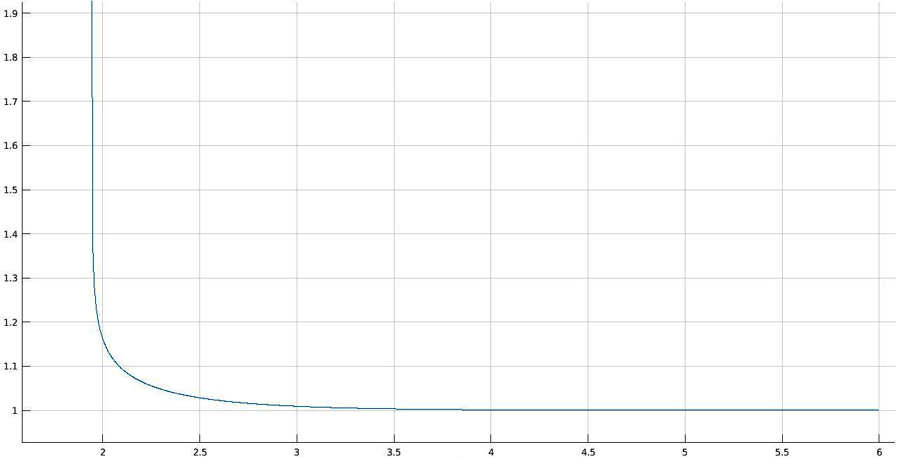
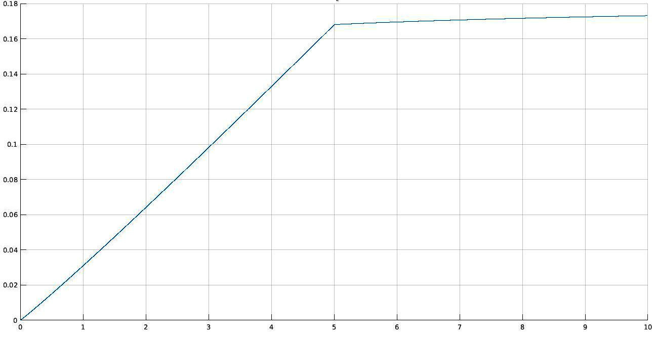
Figure 1. On the left, the graph of $\displaystyle\delta\mapsto M_{\delta}$ when $\displaystyle\lambda=1$ ; on the right, the evolution of $\displaystyle\varepsilon\mapsto b(\varepsilon)$ for $\displaystyle\lambda=1$ and $\displaystyle\delta=2$

This curve is, as expected, non-decreasing (remark that it is not linear by parts) : the smaller $\displaystyle\varepsilon$, the smaller $\displaystyle b(\varepsilon)$ : the result will hold only for very small perturbations $\displaystyle b$ of the reference process.

5.1.2. About the choice of $\displaystyle\delta$

For now, fix $\displaystyle\lambda=1$. Here, we are interested in the optimal value for $\displaystyle\delta$, that is the $\displaystyle\delta$ which allows the largest possible window of choice for $\displaystyle\|b\|_{\infty}$ in order to satisfy proposition 2.

For instance, we set $\displaystyle\varepsilon=1$ and $\displaystyle a=a_{1}$. Then, considering $\displaystyle b_{1}:=b(1)$ as a function of $\displaystyle\delta$, we have :

$$b_{1}(\delta)=\frac{1}{2\sqrt{2e}(8!)^{1/8}}\left(\delta\;M_{\delta}^{7/4}\left(1-\frac{C_{P}}{8\delta}\ln\left(\frac{2M_{\delta}^{4}+1}{16M_{\delta}^{8}}\left(\sqrt{1+\frac{1}{32(1+2M_{\delta}^{4})^{2}}}-1\right)\right)\right)\right)^{-1/2}$$

with $\displaystyle M_{\delta}=(1-e^{-2\delta})^{-3/8}(1-50e^{-2\delta}+49e^{-4\delta})^{-1/16}$.

We wish to determine,

$$\delta_{*}=\underset{\delta>\ln(7)}{\text{argmax}}\;b_{1}(\delta)$$

i.e. the value of $\displaystyle\delta$ for which proposition 1 will be satisfied for the largest value of $\displaystyle\|b\|_{\infty}$.

Differentiating $\displaystyle b_{1}$ with respect to $\displaystyle\delta$ in order to find the points where the derivative vanishes looks a rather hopeless case.

We can nevertheless draw the graph of $\displaystyle b_{1}$ in figure 2 : there seems to be a clear maximum, in this case for $\displaystyle\delta$ close to $\displaystyle 2.22$, with a upper-bound for $\displaystyle\|b\|_{\infty}$ around $\displaystyle 0.0325$.

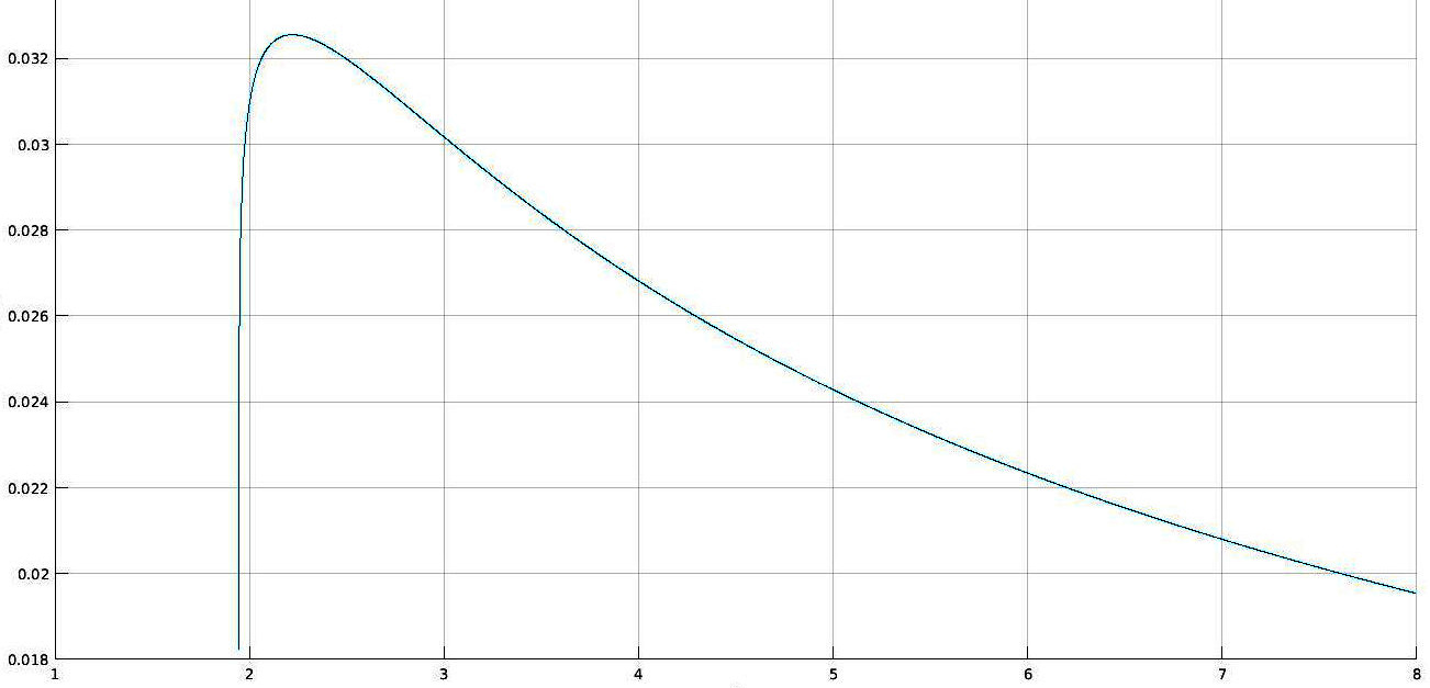
Figure 2. $\displaystyle b_{1}$ as a function of $\displaystyle\delta$ with $\displaystyle\lambda=1$

Other values of $\displaystyle\lambda$ provide similar representations, on a different scale. We observe a surprising correlation, at least at first glance, when looking for the corresponding values for other choices of $\displaystyle\lambda$ ; they are gathered in the following table :

$\displaystyle\begin{array}[]{|c|c|c|c|c|c|c|c|c|}\hline\cr\lambda&0.01&0.1&0.5&1&2&5&10&100\\ \hline\cr\delta_{*}&222&22.2&4.44&2.22&1.11&0.44&0.222&0.0222\\ \hline\cr b_{1}(\delta_{*})&0.00325&0.0103&0.0230&0.0325&0.0460&0.0728&0.103&0.325\\ \hline\cr\end{array}$

From this, we can conjecture approximate links between $\displaystyle\lambda$, $\displaystyle\delta_{*}$ and $\displaystyle b_{1}(\delta_{*})$ : it seems that, one the one hand,

(51) $$\delta_{*}\simeq\frac{2.220296}{\lambda}$$

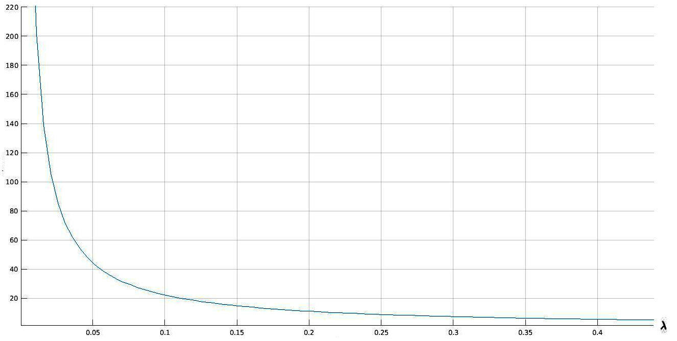
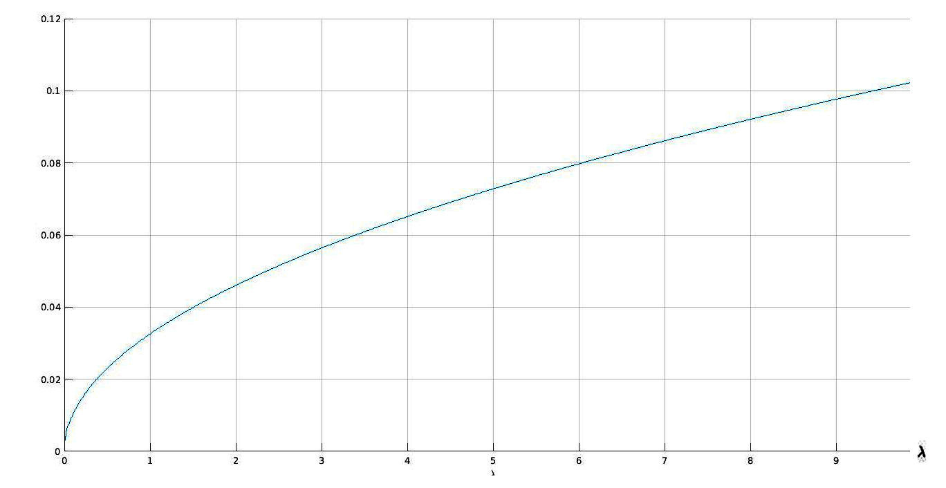
Figure 3. On the left, the optimal value of $\displaystyle\delta$, $\displaystyle\delta_{*}$, as a function of $\displaystyle\lambda$; on the right, the optimal bound $\displaystyle b_{1}(\delta_{*})$, depending on $\displaystyle\lambda$

and, on the other hand,

(52) $$b_{1}(\delta_{*})\simeq 0.3255108\sqrt{\lambda}\simeq\frac{0,04850326}{\sqrt{\delta_{*}}}$$

Thus, we conjecture that the larger $\displaystyle\lambda$ (and thus the reference drift term), the smaller $\displaystyle\delta$ and the larger $\displaystyle b_{1}(\delta_{*})$ (and thus a larger window of possibilities for the perturbation $\displaystyle b$).

Remark 13.

The so-called optimal bound for $\displaystyle\|b\|_{\infty}$, that is $\displaystyle b_{1}(\delta_{*})$, is the one discusses in Proposition 1, and is not linked with the one, unknown, that appears in Theorem 2, about which, as previously mentioned, we are not able to say anything.

Acknowledgements : I would like to thank Sylvie Roelly for her sustained help during the writing of this paper.

References

- [1] C. Ané, S Blachère, D. Chafaï, P. Fougères, I. Gentil, F. Malrieu, C. Roberto, and G. Scheffer. Sur les inégalités de Sobolev logarithmiques. Société mathématique de France, 2000.
- [2] P. Cattiaux, D. Chafaï, and A. Guillin. Central limit theorems for additive functionals of ergodic Markov diffusions processes. Latin American Journal of Probability and Mathematical Statistics, 9(2):337–82, 2012.
- [3] P. Cattiaux, A. Guillin, and P.A. Zitt. Poincaré inequality and hitting times. Ann. Institut Henri Poincaré, 49(1):95–118, 2013.
- [4] P. Dai Pra and S. Roelly. An existence result for infinite-dimensional Brownian diffusions with non-regular and non-Markovian drift. Markov Processes Relat. Fields, 10:113–136, 2004.
- [5] P. Dai Pra, S. Roelly, and H. Zessin. A Gibbs variatonal principle in space-time for infinite-dimensional diffusions. Proba. Theory Relat. Fields, 122(2):289–315, 2002.
- [6] S-Y. Ha, K. Lee, and D. Levy. Emergence of time-asymptotic flocking in a stochastic Cucker-Smale system. Communications in Mathematical Sciences, 7(2):453–69, 2009.
- [7] I. Ignatyuk, V.A. Malyshev, and V. Sidoravicius. Convergence of hte stochatic quantization method. I. Theory Probab. Appl., 37(2):209–21, 1992.
- [8] K. Itô and M. Nisio. On stationary solutions of a stochastic differential equation. J. Math. Kyoto Univ., 4(1):1–75, 1964.
- [9] A.F. Ivanov, Y.I. Kazmerchuk, and A.V. Swishchuk. Theory, Stochastic Stability and Applications of Stochastic Delay Differential Equations: a Survey of Recent Results. Differential Equations and Dynamical Systems, 11:55–115, 2003.
- [10] C. Kipnis and S.R.S. Varadhan. Central limit theorem for additive functionals of reversible Markov processes and applications to simple exclusions. Comm. Math. Phys., 104(1):1–19, 1986.
- [11] A. Kolmogorov. Zur Umkehrbarkeit der statistischen Naturgesetze. Mathematische Annalen, 113(1):766–72, 1937.
- [12] R.S. Lipster and A.N. Shiryayev. Statistics of Random Processes I, General Theory. Springer-Verlag, 1977.
- [13] V.A. Malyshev and R.A. Minlos. Gibbs Random Fields, Cluster Expansions. Kluwer, 1991.
- [14] R.A. Minlos, S. Roelly, and H. Zessin. Gibbs states on space-time. Potential Annal., 13(4):367–408, 2000.
- [15] R.A. Minlos, A. Verbeure, and V. Zagrebnov. A quantum cristal model in the light mass limit : Gibbs states. Rev. Math. Phys., 12(7):981–1032, 2000.
- [16] S. Roelly and W.M. Ruszel. Propagation of Gibbsianness for Infinite-Dimensional Diffusions with Space-Time Interaction. Markov Processes Relat. Fields, 20:653–74, 2014.
- [17] S. Roelly and M. Sortais. Space-time asymptotics of an infinite-dimensional diffusion having a long-range memory. Markov Processes Relat. Fields, 10:653–86, 2004.