Low-Complexity Sub-band Digital Predistortion for Spurious Emission Suppression in Noncontiguous Spectrum Access

Abstract

Noncontiguous transmission schemes combined with high power-efficiency requirements pose big challenges for radio transmitter and power amplifier (PA) design and implementation. Due to the nonlinear nature of the PA, severe unwanted emissions can occur, which can potentially interfere with neighboring channel signals or even desensitize the own receiver in frequency division duplexing (FDD) transceivers. In this article, to suppress such unwanted emissions, a low-complexity sub-band DPD solution, specifically tailored for spectrally noncontiguous transmission schemes in low-cost devices, is proposed. The proposed technique aims at mitigating only the selected spurious intermodulation distortion components at the PA output, hence allowing for substantially reduced processing complexity compared to classical linearization solutions. Furthermore, novel decorrelation based parameter learning solutions are also proposed and formulated, which offer reduced computing complexity in parameter estimation as well as the ability to track time-varying features adaptively. Comprehensive simulation and RF measurement results are provided, using a commercial LTE-Advanced mobile PA, to evaluate and validate the effectiveness of the proposed solution in real world scenarios. The obtained results demonstrate that highly efficient spurious component suppression can be obtained using the proposed solutions.

I Introduction

Spectrum scarcity and ever-increasing data rate requirements are the two main motivating factors behind introducing carrier aggregation (CA) in modern wireless communication systems, such as 3GPP LTE-Advanced [1, 2]. In CA transmission, multiple component carriers (CCs) at different RF frequencies are adopted simultaneously, either within the same RF band (intraband CA), or at different RF bands (interband CA) [3]. While interband CA naturally leads to a non-contiguous transmit spectrum, this can also happen in the intraband CA case when the adopted component carriers are located in a non-contiguous manner. Adopting non-contiguous CA provides lots of flexibility in RF spectrum use, but also poses substantial challenges in the transmitter design, especially in lower-cost devices such as LTE-Advanced user equipment (UE). Moreover, multicarrier type modulations with very large peak-to-average power ratio (PAPR) are used in most state-of-the-art wireless communication systems. When combined with noncontiguous transmission schemes and high power-efficiency requirements, controlling the transmitter unwanted emissions due to power amplifier (PA) nonlinearity becomes a true challenge [4, 5, 6].

In [3], a comparison of different transmitter architectures for CA based transmission schemes was presented, showing that it is more power efficient to combine the CCs before the PA, and thus use only a single PA, instead of having a separate PA for each CC. This is also technically feasible, especially in the intraband CA case. The power savings can be quite significant since the overall transmitter efficiency is dominated by the PA [3], and is particularly critical in mobile terminals and other lower-cost devices, such as small-cell base-stations, with limited computing and cooling capabilities [7, 8]. However, the power efficiency gained from using a single PA for all CCs comes at the expense of more severe unwanted emissions, stemming from the PA nonlinear characteristics, that can occur at adjacent channels or bands, or even at own receiver band in FDD transceiver case [4, 5, 6, 9].

The levels of different unwanted emissions are, in general, regulated by the standardization bodies and ITU-R [10]. It has been recently demonstrated that in the context of LTE-Advanced mobile transmitter with noncontiguous CA or multicluster type transmission, the PA nonlinearities lead to spurious emissions that can seriously violate the given spectrum and spurious emission limits if not properly controlled [2, 4, 5, 6]. Furthermore, in FDD devices, in addition to violating the general spurious emission limits, the generated spurious components can also overlap with the device’s own receive band, causing own receiver desensitization [4, 9, 11, 12]. One obvious solution to decrease the levels of unwanted emissions is to back off the transmit power from its saturation region. In 3GPP UE terminology, this is known as Maximum Power Reduction (MPR), and MPR values up to 16 dB are allowed in some use cases for mobile terminals [2]. However, this approach will end up yielding a significantly lower PA efficiency as well as a substantial reduction in the network coverage. There is thus a clear need for alternative PA linearization solutions which do not have such drastic adverse effects.

Digital predistortion (DPD) is, in general, one of the most effective solutions for mitigating transmitter nonlinear distortion. There have been substantial research efforts in the past 20 years in developing ever more efficient and elaborate DPD techniques, mostly for high-end macro base-station type of devices. The conventional DPD approaches seek to linearize the full composite transmit signal, and we thus refer to such solutions as full-band DPD in this article. There have also been a handful of recent works on efficient concurrent linearization techniques for multi-band transmitters that employ only a single PA [13, 14, 15]. These works assume that the component carriers are separated by a large distance such that the spurious emissions are filtered out by the transmit RF filter, and hence linearization of only the main carriers is pursued.

Complementary to such methods, the scope of this paper is to introduce a low-complexity DPD solution for suppressing the spurious emissions in non-contiguous transmission cases, while not concentrating specifically on the linearization of the main component carriers. Hereafter, we will refer to such linearization solutions as sub-band DPD. This approach is motivated by the following two factors. First, the emission limits in the spurious region are generally stricter than in the spectral regrowth region around the component carriers, and are thus more easily violated. This has been recognized also in 3GPP recently, in the context of intraband noncontiguous carrier aggregation [2, 4, 5, 6]. Moreover, even in interband carrier aggregation scenarios in FDD devices, some of the spurious components can be hitting the own RX band causing own receiver desensitization [11]. Second, by concentrating the linearization efforts to the most critical spurious emissions only, the processing and instrumentation requirements can be significantly relaxed, thus potentially facilitating the DPD processing also in mobile terminals and other lower-cost devices. This applies not only to the DPD main path processing complexity but also to the feedback receiver instrumentation complexity which can also be substantially reduced.

There have been some recent studies in the literature that consider the mitigation of the spurious emissions explicitly. In [16, 17, 18], such processing was added to complement a concurrent linearization system while assuming a frequency-flat PA response within the spurious sub-band. In [16, 17], the DPD parameter estimation was done offline, based on extracting the quasi-memoryless PA parameters using large-signal network analyzer (LSNA) measurements, and covering up to fifth-order processing. In [18], a memoryless least-squares fit between the observed intermodulation distortion (IMD) at the considered sub-band and certain basis functions was performed. The basis functions were generated using a wideband composite carrier baseband equivalent signal, followed by sub-band filtering, implying a very high sample rate and processing complexity, especially for widely spaced carriers. The estimated and regenerated IMD was then applied at the PA input, oppositely phased, such that it is canceled at the PA output. In [19, 20], on the other hand, third-order nonlinearities at the IM3 sub-bands were specifically targeted, through explicit, low-rate, behavioral modeling of the baseband equivalent IM3 sub-band emissions. Furthermore, the parameter estimation of the DPD was based on a closed-loop feedback with a decorrelation-based learning rule, which was shown to have better linearization performance compared to the third-order inverse solution in [16] in terms of the spurious emission suppression. Moreover, an FPGA implementation of this third-order decorrelation-based sub-band DPD was presented in [21], demonstrating fast and reliable performance under real time constraints. A recent overview article [22] highlighted the main principles and advantages of such low complexity sub-band DPD solutions, while not concentrating on the details of the DPD processing or parameter estimation and adaptation algorithms at technical level. In [23], on the other hand, a flexible full-band DPD solution was also proposed by the authors which can optimize the DPD coefficients to minimize the nonlinear distortion at a particular frequency or sub-band in the out-of-band or spurious regions. However, like other full-band DPD techniques, it requires very high sampling rates in the transmitter and feedback receiver when the carrier spacing between the CCs increases.

In this article, we extend the elementary third-order IM3 sub-band DPD solution, proposed by the authors in [19, 20], in two ways. First, the third-order IM3 sub-band DPD is extended to incorporate higher-order processing based on explicit modeling of the higher-order spurious components at the IM3 sub-band. This will enhance the IM3 spurious emission suppression considerably. Furthermore, we also extend the sub-band DPD solution to include higher-order sub-bands, i.e., IM5, IM7, etc., thus offering more flexibility and linearization capabilities beyond the basic IM3 sub-band. All the proposed solutions are derived for wideband nonlinear PAs with memory. Furthermore, we also formulate novel decorrelation-based parameter estimation methods, covering both sample-adaptive and block-adaptive learning rules, to efficiently identify the needed DPD parameters with low complexity. The proposed learning solutions are also shown to offer better performance than the earlier proposed third-order or fifth-order inverse based methods. We also provide comprehensive simulation and RF measurement results, using a commercial LTE-Advanced mobile PA, to evaluate and validate the effectiveness of the proposed solutions in real world scenarios.

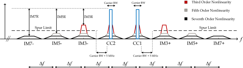
Figure 1: Illustration of different intermodulation distortion components created by a nonlinear PA when excited with a non-contiguous CA signal with two component carriers. Here, nonlinear distortion components up to order 7 are shown.

The rest of this article is organized as follows: Section II presents the mathematical modeling of the different considered spurious components at different sub-bands, produced by a nonlinear PA with memory. Stemming from this modeling, also the corresponding core processing principles of the proposed DPD solutions at different sub-bands are formulated. Then, Section III presents the proposed DPD parameter learning solutions, covering both sample-adaptive and block-adaptive decorrelation solutions at different sub-bands. Section IV addresses then different implementation alternatives of the proposed sub-band DPD concept, and also analyzes the computing complexity of the sub-band DPD in terms of the number of floating point operations together with some hardware complexity aspects. Finally, Sections V and VI report comprehensive simulation and RF measurement results, evidencing excellent spurious emission suppression in different realistic scenarios.

II Spurious Component Modeling and Proposed Sub-band DPD Processing

In this manuscript, we assume a practical case of non-contiguous carrier aggregation with two component carriers. When such noncontiguous dual-carrier signal is applied at the PA input, the PA nonlinearity leads to intermodulation distortion at different sub-bands, as shown in Fig. 1. Assuming a CC separation of $\Delta f$, in addition to the spectral regrowth around the main carriers, intermodulation between the two CCs yields strong IMD at integer multiples of $\Delta f$ from the main CCs. In this article, we refer to the intermodulation (IM) sub-bands located at $\pm\Delta f$ from the main CCs as the IM3 sub-bands. Similarly, the IM5 sub-bands are located at $\pm 2\Delta f$ from the main CCs, and so on. In general, each IM sub-band includes nonlinear distortion components of different orders as shown in Fig. 1. For example, in the case of a seventh-order PA nonlinearity, the IM3 sub-band contains third, fifth and seventh-order nonlinearities, while the IM5 sub-band contains fifth and seventh-order components.

In this section, we start with the fundamental modeling of the nonlinear distortion at the IM3 sub-band as a concrete example. Stemming from that modeling, we then formulate the basic processing of the proposed IM3 sub-band DPD. After that, the modeling is extended to cover the nonlinear distortion components at the higher-order IM sub-bands, followed by the corresponding higher-order sub-band DPD processing. The actual parameter estimation and learning algorithms for the proposed sub-band DPD structures are then presented in details in Section III. In all the modeling and developments, we adopt the widely-used wideband Parallel Hammerstein (PH) PA model [24] to describe the fundamental nonlinear behavior of the PA, as it has been shown to model accurately the measured nonlinear behavior of different classes of true PAs.

II-A Spurious Component Modeling at IM3 Sub-bands

The modeling is carried out at composite baseband equivalent level, where the two component carriers are assumed to be separated by $2f_{IF}$. The composite baseband equivalent input and output signals of the $P^{th}$ order Parallel Hammerstein PA model, with monomial nonlinearities and FIR branch filters, respectively, read

$$x(n) =x_{1}(n)e^{j2\pi\frac{f_{IF}}{f_{s}}n}+x_{2}(n)e^{-j2\pi\frac{f_{IF}}{f_{s}}n},$$ (1)

$$y(n) =\sum_{\begin{subarray}{c}p=1\\ p\text{ odd}\end{subarray}}^{P}f_{p,n}\star|x(n)|^{p-1}x(n),$$ (2)

where $x_{1}(n)$ and $x_{2}(n)$ are the baseband component carrier signals, $f_{p,n}$ denotes the PH branch filter impulse responses of order $p$, and $\star$ is the convolution operator. Intermodulation between the two component carriers leads to the appearance of IMD components at $\pm 3f_{IF}$, $\pm 5f_{IF}$, etc., as shown in Fig. 1 for the corresponding RF spectrum.

As a concrete example, let us analyze the IMD at $\pm 3f_{IF}$. Direct substitution of (1) in (2) allows extracting the baseband equivalent distortion terms at the IM3 sub-bands, which, through straight-forward manipulations, yields

$$y_{IM3_{\pm}}(n)=\sum_{\begin{subarray}{c}p=3\\ p\text{ odd}\end{subarray}}^{P}f_{3\pm,p,n}\star u_{3\pm,p}(n).$$ (3)

Here, $f_{3\pm,p,n}$ denote the baseband equivalent impulse responses corresponding to the wideband PH PA model filters $f_{p,n}$, evaluated at the IM3$\pm$ sub-bands, formally defined as

$$f_{3\pm,p,n} =LPF\{e^{\mp j2\pi\frac{3f_{IF}}{f_{s}}n}f_{p,n}\},$$ (4)

with $LPF\{.\}$ denoting an ideal low pass filtering operation with a passband width $P$ times the bandwidth of the wider CC. Furthermore, $u_{3+,p}(n)$ and $u_{3-,p}(n)$ in (3) are the corresponding $p^{th}$ order static nonlinear (SNL) basis functions, related to the nonlinear distortion at the IM3+ and IM3- sub-bands, respectively. Assuming then an $11^{th}$ order PA model (i.e., $P=11$), as a concrete high-order example, the IM3+ sub-band basis functions read

$$u_{3+,3}(n) =x_{2}^{*}(n)x_{1}^{2}(n)$$ (5)

$$u_{3+,5}(n) =u_{3+,3}(n)\times(2|x_{1}(n)|^{2}+3|x_{2}(n)|^{2})$$ (6)

$$u_{3+,7}(n) =u_{3+,3}(n)\times(3|x_{1}(n)|^{4}+6|x_{2}(n)|^{4}$$

$$+12|x_{1}(n)|^{2}|x_{2}(n)|^{2})$$ (7)

$$u_{3+,9}(n) =u_{3+,3}(n)\times(4|x_{1}(n)|^{6}+10|x_{2}(n)|^{6}$$

$$+30|x_{1}(n)|^{4}|x_{2}(n)|^{2}+40|x_{1}(n)|^{2}|x_{2}(n)|^{4})$$ (8)

$$u_{3+,11}(n) =u_{3+,3}(n)\times(5|x_{1}(n)|^{8}+15|x_{2}(n)|^{8}$$

$$+60|x_{1}(n)|^{6}|x_{2}(n)|^{2}+100|x_{1}(n)|^{2}|x_{2}(n)|^{6}$$

$$+150|x_{1}(n)|^{4}|x_{2}(n)|^{4}).$$ (9)

The corresponding basis functions for the IM3- sub-band, i.e., $u_{3-,p}(n)$, can be obtained by simply interchanging $x_{1}(n)$ and $x_{2}(n)$ in the above expressions. Next, these behavioral modeling results are utilized to formulate the proposed IM3 sub-band DPD concept, specifically tailored to suppress the distortion at the IM3 sub-band.

II-B Proposed IM3 Sub-band DPD Principle

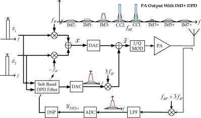
Figure 2: The proposed sub-band DPD processing principle focusing on the IM3+ sub-band. Thick lines are used to indicate complex I/Q processing. For presentation simplicity, TX filtering between the feedback coupler and the antenna is not shown.

For presentation purposes, we focus here on suppressing the spurious emissions at the IM3+ sub-band, while the corresponding emissions at the IM3- sub-band can also be easily mitigated using a very similar structure with minor changes as will be elaborated later in Section II-C. The key idea of the sub-band DPD concept is to inject a proper additional low-power cancellation signal, with structural similarity to (3) and located at $+3f_{IF}$, into the PA input, such that the level of the IM3+ term at the PA output is reduced. Now, stemming from the IMD structure in (3), an appropriate digital injection signal can be obtained by adopting the IM3+ basis functions $u_{3+,p}(n)$ in (5)-(9), combined with proper filtering using a bank of sub-band DPD filters $\alpha_{3+,p,n}$. Incorporating such sub-band DPD processing with polynomial order $Q$, the composite baseband equivalent PA input signal reads

$$\tilde{x}(n) =x(n)+\left[\sum_{\begin{subarray}{c}p=3\\ p\text{ odd}\end{subarray}}^{Q}\alpha_{3+,p,n}\star u_{3+,p}(n)\right]e^{j2\pi\frac{3f_{IF}}{f_{s}}n}$$ (10)

Here, and in the continuation, we use $\tilde{(.)}$ variables to indicate sub-band DPD processing and the corresponding predistorted signals. This DPD processing principle is illustrated in Fig. 2 at a conceptual level, where the TX/RX duplexer filters are omitted for simplicity of the presentation since they do not directly impact the sub-band DPD processing or learning. Similar convention is followed also in other figures. Different implementation alternatives as well as the parameter learning and feedback receiver aspects are addressed in more details in Sections III and IV.

II-C Generalization to Higher-Order IM Sub-bands

The direct substitution of (1) in (2) leads to the appearance of spurious intermodulation terms also at higher-order IM sub-bands, in addition to the previously considered IM3 sub-bands, as illustrated already in Fig. 1. These higher-order sub-band emissions can also be harmful, since they can violate the emission limits, cause own receiver desensitization, or both. Thus, developing a sub-band DPD solution that can tackle also the distortion at these higher-order IM sub-bands with feasible complexity is important. Similar to the above IM3+ sub-band developments, we next extract the IMD terms at the higher-order IM sub-bands. The baseband equivalent IMD terms at the IM5+, IM7+, IM9+, and IM11+ sub-bands, as concrete examples, can be extracted using (1) and (2), interpreted at proper sub-bands, yielding

$$y_{IM5_{+}}(n) =\sum_{\begin{subarray}{c}p=5\\ p\text{ odd}\end{subarray}}^{P}f_{5+,p,n}\star u_{5+,p}(n)$$ (11)

$$y_{IM7_{+}}(n) =\sum_{\begin{subarray}{c}p=7\\ p\text{ odd}\end{subarray}}^{P}f_{7+,p,n}\star u_{7+,p}(n)$$ (12)

$$y_{IM9_{+}}(n) =\sum_{\begin{subarray}{c}p=9\\ p\text{ odd}\end{subarray}}^{P}f_{9+,p,n}\star u_{9+,p}(n)$$ (13)

$$y_{IM11_{+}}(n) =\sum_{\begin{subarray}{c}p=11\\ p\text{ odd}\end{subarray}}^{P}f_{11+,p,n}\star u_{11+,p}(n).$$ (14)

In the above models, $f_{5+,p,n}$, $f_{7+,p,n}$, $f_{9+,p,n}$, and $f_{11+,p,n}$ denote the baseband equivalent impulse responses corresponding to the wideband PA model filters $f_{p,n}$ in (2), evaluated at the IM5+, IM7+, IM9+, and IM11+ sub-bands, respectively. These are formally obtained similar to (4) but replacing $3f_{IF}$ with either $5f_{IF}$, $7f_{IF}$, $9f_{IF}$, or $11f_{IF}$, respectively. The $p^{th}$ order basis functions at the these higher-order IM sub-bands, denoted by $u_{5+,p}(n)$, $u_{7+,p}(n)$, $u_{9+,p}(n)$, and $u_{11+,p}(n)$, and assuming again an $11^{th}$ order PH PA model, read

$$u_{5+,5}(n) =(x_{2}(n)^{*})^{2}x_{1}(n)^{3}$$ (15)

$$u_{5+,7}(n) =u_{5+,5}(n)(4|x_{2}(n)|^{2}+3|x_{1}(n)|^{2})$$ (16)

$$u_{5+,9}(n) =u_{5+,5}(n)(10|x_{2}(n)|^{4}+6|x_{1}(n)|^{4}$$

$$+20|x_{1}(n)|^{2}|x_{2}(n)|^{2})$$ (17)

$$u_{5+,11}(n) =u_{5+,5}(n)(20|x_{2}(n)|^{6}+10|x_{1}(n)|^{6}$$

$$+75|x_{2}(n)|^{4}|x_{1}(n)|^{2}+60|x_{2}(n)|^{2}|x_{1}(n)|^{4})$$ (18)

$$u_{7+,7}(n) =(x_{2}(n)^{*})^{3}x_{1}(n)^{4}$$ (19)

$$u_{7+,9}(n) =u_{7+,7}(n)(5|x_{2}(n)|^{2}+4|x_{1}(n)|^{2})$$ (20)

$$u_{7+,11}(n) =u_{7+,7}(n)(15|x_{2}(n)|^{4}+10|x_{1}(n)|^{4}$$

$$+30|x_{2}(n)|^{2}|x_{1}(n)|^{2})$$ (21)

$$u_{9+,9}(n) =(x_{2}(n)^{*})^{4}x_{1}(n)^{5}$$ (22)

$$u_{9+,11}(n) =u_{9+,9}(n)(6|x_{2}(n)|^{2}+5|x_{1}(n|^{2})$$ (23)

$$u_{11+,11}(n) =(x_{2}(n)^{*})^{5}x_{1}(n)^{6}.$$ (24)

The corresponding baseband equivalent IMD terms at the negative IM sub-bands can be obtained by simply interchanging $x_{1}(n)$ and $x_{2}(n)$ in (15)-(24).

Then, stemming from the distortion structure in (11)-(14), and adopting similar ideology as in the previous IM3 sub-band DPD case, a natural injection signal for suppressing the spur components at higher-order IM sub-bands can be obtained by properly filtering and combining the above higher-order sub-band basis functions. The sub-band specific filters for the $p^{th}$ order basis functions are denoted with $\alpha_{5+,p,n}$, $\alpha_{7+,p,n}$, $\alpha_{9+,p,n}$, and $\alpha_{11+,p,n}$. Incorporating such DPD processing with DPD polynomial order $Q$, and aggregating at the same time parallel sub-band DPDs simultaneously for the IM3+, IM5+, and IM7+ sub-bands, as a concrete example, the composite baseband equivalent PA input signal now reads

$$\tilde{x}(n)=x(n) +\left[\sum_{\begin{subarray}{c}p=3\\ p\text{ odd}\end{subarray}}^{Q}\alpha_{3+,p,n}\star u_{3+,p}(n)\right]e^{j2\pi\frac{3f_{IF}}{f_{s}}n}$$

$$+\left[\sum_{\begin{subarray}{c}p=5\\ p\text{ odd}\end{subarray}}^{Q}\alpha_{5+,p,n}\star u_{5+,p}(n)\right]e^{j2\pi\frac{5f_{IF}}{f_{s}}n}$$

$$+\left[\sum_{\begin{subarray}{c}p=7\\ p\text{ odd}\end{subarray}}^{Q}\alpha_{7+,p,n}\star u_{7+,p}(n)\right]e^{j2\pi\frac{7f_{IF}}{f_{s}}n}$$ (25)

In general, the achievable suppression of the distortion at different IM sub-bands depends directly on the selection and optimization of the different filters $\alpha_{3+,p,n}$, $\alpha_{5+,p,n}$, $\alpha_{7+,p,n}$, and so on. This is addressed in detail in the next section.

III Sub-band DPD Parameter Learning Using the Decorrelation Principle

In this section, based on the previous spurious component modeling and the proposed sub-band DPD principle, we formulate computing feasible and highly efficient estimation algorithms for learning and optimizing the sub-band DPD filter coefficients such that the spurious emissions are minimized at the considered IM sub-bands. We start by deriving some analytical reference solutions, taking the third-order IM3 sub-band DPD as a simple and tractable example, in order to demonstrate that minimizing the IM3 power is essentially identical to decorrelating the IM3 observation against the corresponding sub-band DPD basis functions. Then, both sample-adaptive and block-adaptive decorrelation based learning rules are devised, covering the general cases of higher-order processing with memory at IM3 and higher-order IM sub-bands.

III-A Analytical Reference Solutions

In this subsection, we derive three analytical reference solutions for calculating the IM3 sub-band DPD coefficients. The considered approaches are the third-order inverse solution, also adopted in [16], the IM3 power minimization solution, and the analytical IM3 decorrelation-based solution. To keep the analytical developments simple and tractable, we consider a simplified case with a third-order memoryless IM3+ sub-band DPD and a third-order memoryless PA. The actual sample-adaptive and block-adaptive decorrelation based learning solutions, devised later in this section, are formulated for the general cases of higher-order processing with memory.

Now, starting with the dual carrier signal in (1), and limiting the study to the simplified case of a third-order memoryless IM3+ sub-band DPD and a third-order memoryless PA, the basic signal models are given by (26)-(30).

$$y(n) =f_{1}x(n)+f_{3}|x(n)|^{2}x(n),$$ (26)

$$u(n) =x_{2}^{*}(n)x_{1}^{2}(n),$$ (27)

$$y_{IM3_{+}}(n) =f_{3}u(n),$$ (28)

$$\tilde{x}(n) =x(n)+\alpha u(n)e^{j2\pi\frac{3f_{IF}}{f_{s}}n},$$ (29)

$$\tilde{y}_{IM3_{+}}(n) =(f_{3}+f_{1}\alpha)u(n)+2f_{3}\alpha(|x_{1}(n)|^{2}+|x_{2}(n)|^{2})u(n)$$

$$+f_{3}|\alpha|^{2}\alpha|x_{1}(n)|^{4}|x_{2}(n)|^{2}u(n).$$ (30)

Here, $f_{1}$ and $f_{3}$ are the memoryless PA model parameters, $\alpha$ denotes the memoryless sub-band DPD parameter to be optimized, while ${y}_{IM3_{+}}(n)$ and $\tilde{y}_{IM3_{+}}(n)$ refer to the baseband equivalent PA output at the positive IM3 sub-band without and with sub-band DPD, respectively.

Now, as (30) clearly shows, the IM3 sub-band distortion at the PA output, with DPD adopted, depends directly on, and can thus be controlled by, the DPD coefficient $\alpha$. In the well-known third-order inverse solution, the DPD parameter $\alpha$ is selected such that the third-order term in (30) is canceled, i.e., $f_{3}+f_{1}\alpha=0$. The corresponding solution, denoted by $\alpha_{inv}$, thus reads

$$\alpha_{inv} =-f_{3}/f_{1}.$$ (31)

However, this will not remove all the distortion, because higher-order terms will be created due to the predistortion, as shown in (30).

A more elaborate method for selecting the DPD parameter $\alpha$ is the one that minimizes the power of the total IM3 sub-band signal, $\tilde{y}_{IM3_{+}}(n)$, referred to as the minimum IM3 power or minimum mean-squared error (MMSE) solution in the continuation. For notational convenience, we define the so-called error signal as $e(n)=\tilde{y}_{IM3_{+}}(n)$, as with ideal predistortion the IM3 sub-band signal would be zero, and thus the optimization means minimizing the power of this error signal. The detailed derivation of the optimum DPD parameter which minimizes the mean squared error ${\rm I\kern-3.00003ptE}[|e(n)|^{2}]$ is given in Appendix A, yielding

$$\alpha_{MMSE}=$$

$$\dfrac{-\left[f_{1}f_{3}^{*}{\rm I\kern-2.70003ptE}_{42}+2|f_{3}|^{2}({\rm I\kern-2.70003ptE}_{62}+{\rm I\kern-2.70003ptE}_{44})\right]^{*}}{\left[|f_{1}|^{2}{\rm I\kern-2.70003ptE}_{42}+4\mathbb{R}(f_{1}f_{3}^{*})({\rm I\kern-2.70003ptE}_{62}+{\rm I\kern-2.70003ptE}_{44})+4|f_{3}|^{2}({\rm I\kern-2.70003ptE}_{46}+2{\rm I\kern-2.70003ptE}_{64}+{\rm I\kern-2.70003ptE}_{82})\right]^{*}},$$ (32)

where ${\rm I\kern-3.00003ptE}_{ij}$ refers to the products of the CC signals’ higher-order moments of the form ${\rm I\kern-3.00003ptE}[|x_{1}|^{i}]{\rm I\kern-3.00003ptE}[|x_{2}|^{j}]$, while ${\rm I\kern-3.00003ptE}[.]$ denotes the statistical expectation operator.

As will be shown with concrete examples in Section V, this MMSE solution provides better linearization performance compared to the third-order inverse solution. However, as shown in (32), the analytical MMSE solution requires the knowledge of various higher-order moments of the CC signals. Furthermore, the above solution is valid only in the case of a memoryless third-order nonlinear system, beyond which obtaining an analytical expression for the DPD coefficients becomes overly tedious. Thus, to relax these constraints, an alternative solution, based on minimizing the correlation between the IM3 sub-band observation and the third-order basis function $u(n)=x_{2}^{*}(n)x_{1}^{2}(n)$ was initially discussed in [19], and will be extended to higher nonlinearity orders and higher-order IM sub-bands in this paper. The analytical reference solution for the decorrelation-based sub-band DPD structure is obtained by setting the correlation between the error signal, $e(n)$, and the third-order basis function, $u(n)=x_{2}^{*}(n)x_{1}^{2}(n)$, to zero, i.e., ${\rm I\kern-3.00003ptE}[e(n)u^{*}(n)]=0$. Then, through straight-forward algebraic manipulations, the decorrelation-based DPD coefficient, denoted by $\alpha_{o}$, can be shown to read

$$\alpha_{o}=\frac{-f_{3}}{f_{1}+2f_{3}(\frac{{\rm I\kern-1.89001ptE}_{60}}{{\rm I\kern-1.89001ptE}_{40}}+\frac{{\rm I\kern-1.89001ptE}_{04}}{{\rm I\kern-1.89001ptE}_{02}})}.$$ (33)

Assuming then, for simplicity, that the CC baseband equivalents are complex Gaussians, (33) simplifies to

$$\alpha_{o}=\frac{-f_{3}}{f_{1}+2f_{3}(3\sigma^{2}_{x,1}+2\sigma^{2}_{x,2})},$$ (34)

where $\sigma^{2}_{x,1}={\rm I\kern-3.00003ptE}[|x_{1}|^{2}]$ and $\sigma^{2}_{x,2}={\rm I\kern-3.00003ptE}[|x_{2}|]^{2}$ are the variances of the two CCs [19].

A clear advantage of the decorrelation-based approach compared to the earlier MMSE solution lies in the simple and straightforward adaptive filtering based practical computing solutions, sketched initially in [19] for simple third-order processing at IM3, which do not require any prior knowledge about signal moments or any other parameters. Furthermore, opposed to the MMSE solution, the decorrelation based approach can be easily extended to include higher-order nonlinearities and memory effects, at both the IM3 sub-band as well as the other higher-order IM sub-bands, as will be described in details in the next subsection.

III-B Sample-Adaptive Decorrelation-based Learning

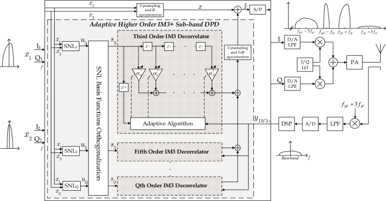
Figure 3: Detailed block diagram of the sample-adaptive decorrelation-based IM3+ sub-band DPD with higher-order nonlinearities and memory.

In this subsection, we provide the actual sample-adaptive learning rules for both IM3 and higher-order IM sub-band DPD structures with memory, whose basic operating principles were described in Section II. To facilitate the learning, we assume a feedback or observation receiver measuring the particular IM sub-band whose sub-band DPD filter coefficients are currently under learning. Notice that opposed to classical wideband DPD principles, where a wideband observation receiver is typically needed, a more narrowband receiver is sufficient here since only the particular IM sub-band is observed. As both the IM3 and the higher-order IM sub-band DPDs are based on multiple strongly correlated basis functions, given in (5)-(9) and (15)-(24), respectively, we start by introducing a basis function orthogonalization procedure, after which the actual proposed adaptive decorrelation algorithms are described.

III-B1 Basis Function Orthogonalization

When a nonlinearity order higher than the IM sub-band order is considered, multiple basis functions are adopted in the sub-band DPD processing, as described in Section II. Taking as an example case the IM3+ sub-band, the SNL basis functions $u_{3+,p}(n)$, $p=1,3,...,Q$, given in (5)-(9), are highly correlated. This can negatively impact the convergence and stability of the adaptive decorrelation-based learning. Therefore, the SNL basis functions are first orthogonalized [25], which yields a new set of DPD basis functions $s_{3+,p}(n)$, $p=1,3,...,Q$, written formally at sample level as

$$\textbf{s}_{3+}(n) =\textbf{W}\textbf{u}_{3+}(n),$$ (35)

where

$$\textbf{u}_{3+}(n) =[u_{3+,3}(n)\>\>u_{3+,5}(n)\>\>...\>\>u_{3+,Q}(n)]^{T},$$ (36)

$$\textbf{s}_{3+}(n) =[s_{3+,3}(n)\>\>s_{3+,5}(n)\>\>...\>\>s_{3+,Q}(n)]^{T},$$ (37)

W $$=\begin{bmatrix}1&0&0&0&0\\ w_{5,3}&w_{5,5}&0&0&0\\ w_{7,3}&w_{7,5}&w_{7,7}&\dots&0\\ \vdots&\vdots&\vdots&\ddots&\vdots\\ w_{Q,3}&w_{Q,5}&w_{Q,7}&\dots&w_{Q,Q}\end{bmatrix}.$$ (38)

The lower triangular matrix W can be obtained, e.g., through Gram-Schmidt orthogonalization, QR or singular value decomposition, or using a lower complexity iterative orthogonalization algorithm [26].

Similarly, the SNL basis functions in (15)-(24) corresponding to the higher-order IM sub-bands are also orthogonalized, to obtain new sets of orthogonal basis functions $\textbf{s}_{5+}(n)$, $\textbf{s}_{7+}(n)$, etc.

III-B2 Adaptive Learning for IM3+ Sub-band

We now present the actual sample-adaptive decorrelation based learning algorithm for the IM3+ sub-band DPD coefficients. For notational convenience, we introduce the following vectors

$$\boldsymbol{\alpha}_{3+,l}(n) =[\alpha_{3+,3,l}(n)\>\>\alpha_{3+,5,l}(n)\>\>...\>\>\alpha_{3+,Q,l}(n)]^{T},$$ (39)

$$\bar{\boldsymbol{\alpha}}_{3+}(n) =[\boldsymbol{\alpha}_{3+,0}(n)^{T}\>\>\boldsymbol{\alpha}_{3+,1}(n)^{T}\>\>...\>\>\boldsymbol{\alpha}_{3+,N}(n)^{T}]^{T},$$ (40)

$$\bar{\textbf{s}}_{3+}(n) =[\textbf{s}_{3+}(n)^{T}\>\>\textbf{s}_{3+}(n-1)^{T}\>\>...\>\>\textbf{s}_{3+}(n-N)^{T}]^{T},$$ (41)

where now $\alpha_{3+,p,l}(n)$ denotes the $l^{th}$ adaptive filter coefficient of the $p^{th}$ order orthogonalized IM3+ basis function $s_{3+,p}(n)$ at time index $n$, and $N$ denotes the adaptive filter memory depth. Furthermore, the vectors $\bar{\boldsymbol{\alpha}}_{3+}(n)$ and $\bar{\textbf{s}}_{3+}(n)$ incorporate all the coefficients and basis function samples up to polynomial order $Q$. Adopting this notation, the instantaneous sample of the composite baseband equivalent PA input signal $\tilde{x}(n)$ now reads

$$\tilde{x}(n) =x(n)+\tilde{x}_{3+}(n)e^{j2\pi\frac{3f_{IF}}{f_{s}}n},$$ (42)

where the instantaneous sample of the baseband equivalent IM3+ injection signal $\tilde{x}_{3+}(n)$ reads

$$\tilde{x}_{3+}(n) =\bar{\boldsymbol{\alpha}}_{3+}(n)^{H}\bar{\textbf{s}}_{3+}(n).$$ (43)

Then, in order to adaptively update the filter coefficients $\bar{\boldsymbol{\alpha}}_{3+}(n)$, the IM3+ sub-band is observed with the feedback receiver, and the coefficient is updated as

$$\bar{\boldsymbol{\alpha}}_{3+}(n+1)=\bar{\boldsymbol{\alpha}}_{3+}(n)-\frac{\mu}{||\bar{\textbf{s}}_{3+}(n)||^{2}+C}\>\bar{\textbf{s}}_{3+}(n)e_{3+}^{*}(n),$$ (44)

where $e_{3+}(n)=\tilde{y}_{IM3_{+}}(n)$ denotes the baseband equivalent observation of the PA output at the IM3+ sub-band with the current DPD coefficients. The scaling factor $||\bar{\textbf{s}}_{3+}(n)||^{2}+C$ normalizing the learning step-size $\mu$ in (44) is philosophically similar to that of the Normalized Least Mean Square (NLMS) algorithm, in effect making the learning characteristics more robust against the input data dynamics.

The proposed coefficient update in (44) is seeking to decorrelate the IM3+ observation and the adopted orthogonalized basis functions. This type of learning algorithm can also be interpreted as a stochastic Newton root search in the objective function $J(\bar{\boldsymbol{\alpha}}_{3+})={\rm I\kern-3.00003ptE}[\tilde{x}_{3+}(n)e_{3+}^{*}(n)]$, where the target is to search for the DPD coefficients $\bar{\boldsymbol{\alpha}}_{3+}$ that minimize the ensemble correlation between $e_{3+}(n)$ and the baseband equivalent of the IM3+ injection signal $\tilde{x}_{3+}(n)$ in (43). The overall processing flow is graphically illustrated in Fig. 3.

III-B3 Adaptive Learning for Higher-Order IM Sub-bands

We now extend the decorrelation based learning to higher-order IM sub-bands. First, adopting vector-based notations again, we introduce the following vectors for notational convenience

$$\boldsymbol{\alpha}_{5+,l}(n) =[\alpha_{5+,5,l}(n)\>\>\alpha_{5+,7,l}(n)\>\>...\>\>\alpha_{5+,Q,l}(n)]^{T},$$ (45)

$$\boldsymbol{\alpha}_{7+,l}(n) =[\alpha_{7+,7,l}(n)\>\>\alpha_{7+,9,l}(n)\>\>...\>\>\alpha_{7+,Q,l}(n)]^{T},$$ (46)

$$\bar{\boldsymbol{\alpha}}_{5+}(n) =[\boldsymbol{\alpha}_{5+,0}(n)^{T}\>\>\boldsymbol{\alpha}_{5+,1}(n)^{T}\>\>...\>\>\boldsymbol{\alpha}_{5+,N}(n)^{T}]^{T},$$ (47)

$$\bar{\boldsymbol{\alpha}}_{7+}(n) =[\boldsymbol{\alpha}_{7+,0}(n)^{T}\>\>\boldsymbol{\alpha}_{7+,1}(n)^{T}\>\>...\>\>\boldsymbol{\alpha}_{7+,N}(n)^{T}]^{T},$$ (48)

$$\textbf{s}_{5+}(n) =[s_{5+,5}(n)\>\>s_{5+,7}(n)\>\>...\>\>s_{5+,Q}(n)]^{T},$$ (49)

$$\textbf{s}_{7+}(n) =[s_{7+,7}(n)\>\>s_{7+,9}(n)\>\>...\>\>s_{7+,Q}(n)]^{T},$$ (50)

$$\bar{\textbf{s}}_{5+}(n) =[\textbf{s}_{5+}(n)^{T}\>\>\textbf{s}_{5+}(n-1)^{T}\>\>...\>\>\textbf{s}_{5+}(n-N)^{T}]^{T},$$ (51)

$$\bar{\textbf{s}}_{7+}(n) =[\textbf{s}_{7+}(n)^{T}\>\>\textbf{s}_{7+}(n-1)^{T}\>\>...\>\>\textbf{s}_{7+}(n-N)^{T}]^{T}.$$ (52)

Then, similar to $\tilde{x}_{3+}(n)$ in (43), the baseband equivalents of the IM5+ and IM7+ sub-band DPD injection signals, denoted by $\tilde{x}_{5+}(n)$ and $\tilde{x}_{7+}(n)$, respectively, read

$$\tilde{x}_{5+}(n)=\bar{\boldsymbol{\alpha}}_{5+}(n)^{H}\bar{\textbf{s}}_{5+}(n),\>\>\tilde{x}_{7+}(n)=\bar{\boldsymbol{\alpha}}_{7+}(n)^{H}\bar{\textbf{s}}_{7+}(n).$$ (53)

Thus, the composite baseband equivalent PA input signal when the IM3+, IM5+, and IM7+ sub-band DPDs are all included, reads

$$\tilde{x}(n)=x(n) +\tilde{x}_{3+}(n)e^{j2\pi\frac{3f_{IF}}{f_{s}}n}+\tilde{x}_{5+}(n)e^{j2\pi\frac{5f_{IF}}{f_{s}}n}$$

$$+\tilde{x}_{7+}(n)e^{j2\pi\frac{7f_{IF}}{f_{s}}n}.$$ (54)

Then, similar to the IM3+ coefficient update in (44), the higher-order IM5+ and IM7+ coefficient updates read

$$\bar{\boldsymbol{\alpha}}_{5+}(n+1) =\bar{\boldsymbol{\alpha}}_{5+}(n)-\frac{\mu}{||\bar{\textbf{s}}_{5+}(n)||^{2}+C}\>\bar{\textbf{s}}_{5+}(n)e_{5+}^{*}(n),$$ (55)

$$\bar{\boldsymbol{\alpha}}_{7+}(n+1) =\bar{\boldsymbol{\alpha}}_{7+}(n)-\frac{\mu}{||\bar{\textbf{s}}_{7+}(n)||^{2}+C}\>\bar{\textbf{s}}_{7+}(n)e_{7+}^{*}(n),$$ (56)

where $e_{5+}(n)=\tilde{y}_{IM5_{+}}(n)$ and $e_{7+}(n)=\tilde{y}_{IM7_{+}}(n)$ denote the baseband equivalents of the PA output at the IM5+ and IM7+ sub-bands, with the corresponding sub-band DPDs included adopting the current coefficients, $\bar{\boldsymbol{\alpha}}_{5+}(n)$ and $\bar{\boldsymbol{\alpha}}_{7+}(n)$, respectively. From the learning perspective, observing a single IM sub-band at a time is the most obvious alternative, which means that the learning for multiple sub-band DPDs happens one at a time. Furthermore, extending the decorrelation-based learning for the negative IM sub-bands is straight-forward. This can be obtained by interchanging $x_{1}(n)$ and $x_{2}(n)$ in the SNL basis functions expressions, and observing the PA output at the corresponding negative IM sub-bands.

III-C Block-Adaptive Decorrelation-based Learning

As Fig. 3 illustrates, the previous sample-adaptive decorrelation-based learning concept is in principle a closed-loop feedback system with nonlinear adaptive processing inside the loop. During the DPD learning phase, and under the potential hardware processing and latency constraints, the DPD parameter convergence and consequently the DPD linearization performance can be affected, especially if the learning loop delay becomes large. Stemming from this, an alternative and new block-adaptive decorrelation-based learning solution is developed next.

The proposed block-adaptive learning rule implies defining two distinct blocks in the processing, as illustrated in Fig. 4. A single update cycle of the learning algorithm will utilize $M$ samples whereas the DPD parameter update interval is $L$ samples, with $M\leq L$. Thus, by proper choice of $M$ and $L$, arbitrarily long loop delays can in principle be tolerated, facilitating stable operation under various hardware and software processing latency constraints. Notice that proper timing synchronization between the observation receiver output and the basis functions is, in general, needed, which can be accomplished prior to executing the actual coefficient learning procedure.

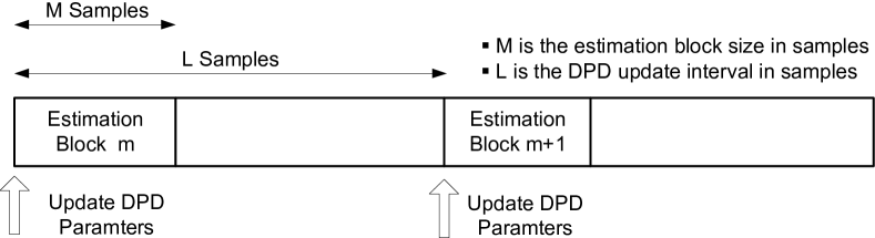
Figure 4: Block-adaptive DPD learning concept. The DPD parameters estimated in the current estimation block $m$ are applied in the sub-band DPD main path processing during the next block.

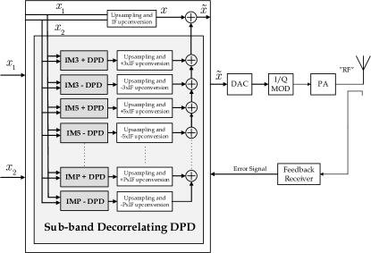
(a) Sub-band DPD Architecture I: Digital IF injection

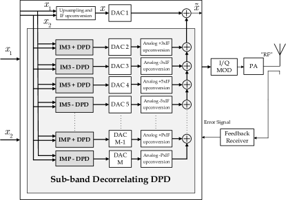
(b) Sub-band DPD Architecture II: Analog IF injection

Figure 5: Overall sub-band DPD architecture with multiple IM sub-bands included. Thick lines indicate complex I/Q processing.

TABLE I: Comparison of running complexities of ninth order sub-band and full-band DPDs. Two 1 MHz CCs with 20 MHz carrier spacing is assumed. DPD sample rate is 189 MSPS for the full-band and 9 MSPS for the sub-band DPD.

	Sub-band DPD				Full-band DPD
	IM3+/- Sub-band	IM5+/- Sub-band	IM7+/- Sub-band	IM9+/- Sub-band	Full-band
Basis Function Generation FLOPs	37	40	45	48	11
DPD Filtering FLOPs	32($N_{1}$+1) - 2	24($N_{1}$+1) - 2	16($N_{1}$+1) - 2	8($N_{1}$+1) - 2	40($N_{2}$+1) - 2
Total Number of FLOPs	32($N_{1}$+1) + 35	24($N_{1}$+1) + 38	16($N_{1}$+1) + 43	8($N_{1}$+1) + 46	40($N_{2}$+1) + 9
GFLOPS ($N_{1}=1$, $N_{2}=3$)	0.891	0.774	0.675	0.558	31.941

Now, assuming an estimation block size of $M$ samples and DPD filter memory depth of $N$ per each of the IM3+ orthogonalized basis functions, the following vectors and matrices, which stack all the samples and the corresponding DPD filter coefficients within block $m$, can be defined:

$$\textbf{s}_{3+}(n_{m}) =[s_{3+,3}(n_{m})\>\>s_{3+,5}(n_{m})\>\>...\>\>s_{3+,Q}(n_{m})]^{T},$$ (57)

$$\bar{\textbf{s}}_{3+}(n_{m}) =[\textbf{s}_{3+}(n_{m})^{T}\>\>...\>\>\textbf{s}_{3+}(n_{m}-N)^{T}]^{T},$$ (58)

$$\textbf{S}_{3+}(m) =[\bar{\textbf{s}}_{3+}(n_{m})\>\>...\>\>\bar{\textbf{s}}_{3+}(n_{m}+M-1)],$$ (59)

$$\boldsymbol{\alpha}_{3+,l}(m) =[\alpha_{3+,3,l}(m)\>\>\alpha_{3+,5,l}(m)\>\>...\>\>\alpha_{3+,Q,l}(m)]^{T},$$ (60)

$$\bar{\boldsymbol{\alpha}}_{3+}(m) =[\boldsymbol{\alpha}_{3+,0}(m)^{T}\>\>\boldsymbol{\alpha}_{3+,1}(m)^{T}\>\>...\>\>\boldsymbol{\alpha}_{3+,N}(m)^{T}]^{T}.$$ (61)

Here, the index of the first sample of block $m$ is denoted by $n_{m}$. The block-adaptive IM3+ sub-band DPD coefficient update then reads

$$\textbf{e}_{3+}(m) =[\tilde{y}_{IM3_{+}}(n_{m})\>\>...\>\>\tilde{y}_{IM3_{+}}(n_{m}+M-1)]^{T},$$ (62)

$$\bar{\boldsymbol{\alpha}}_{3+}(m+1) =\bar{\boldsymbol{\alpha}}_{3+}(m)-\frac{\mu}{||\textbf{S}_{3+}(m)||^{2}+C}\>\textbf{S}_{3+}(m)\textbf{e}_{3+}^{*}(m),$$ (63)

where $\textbf{e}_{3+}^{*}(m)$ refers to the element-wise conjugated error signal vector, while $\textbf{S}_{3+}(m)$ denotes the filter input data matrix, all within the processing block $m$. The obtained new DPD coefficients $\bar{\boldsymbol{\alpha}}_{3+}(m+1)$ are then applied on the next block of $L$ samples as illustrated in Fig. 4. While the above presentation describes the block-adaptive learning only at the IM3+ sub-band, extending the principle to higher-order IM sub-bands is straightforward, and thus not explicitly shown.

IV Implementation Aspects and Complexity Analysis

One of the main advantages of the proposed decorrelation-based sub-band DPD technique is its reduced complexity compared to the classical full-band DPD processing, especially in scenarios where the CCs are widely spaced and thus very high speed ADCs and DACs are required in the classical solutions. In this section, we first address some implementation aspects of the proposed sub-band DPD concept. We then provide a thorough comparison of the computing and hardware complexity perspectives between the full-band and the proposed sub-band DPDs. Finally, some system power efficiency considerations are also presented, with particular focus on low-cost mobile devices.

IV-A Sub-band DPD Implementation Alternatives

Fig. 5 shows two alternative architectures of the overall sub-band DPD processing with multiple IM sub-bands. The first architecture shown in Fig. 5(a) adds an upsampling and digital IF upconversion block after each sub-band DPD stage in order to digitally place the generated injection signals at proper intermediate frequencies. After adding the sub-band DPD outputs in the digital domain, a single wideband DAC per I and Q branch is used after which the signal is upconverted to RF and amplified by the PA.

The second architecture in Fig. 5(b) adds the outputs of the sub-band DPDs in the analog domain, implying that each sub-band DPD is followed by a narrow-band DAC per I and Q branch, together with an analog complex IF upconversion. A common I/Q RF modulator is then used for all sub-bands prior to the PA module.

Both of these two architectures have their own advantages and disadvantages. In particular, if the carrier spacing between the component carriers is not very large, architecture I is likely to be more suitable. On the other hand, when the carrier spacing starts to increase, using a single wideband DAC may not be efficient from cost and power consumption perspectives, so in this case architecture II is likely to be more attractive. However, some extra processing may be required in this architecture in order to achieve proper synchronization between the DACs. This forms an interesting topic for future research.

A common advantage of both architectures is that each sub-band DPD block can be switched on or off according to the prevailing emission levels and limits at the considered sub-bands. Such flexibility is not available in the classical full-band DPD solutions since, by design, a full-band predistorter always tries to linearize the full composite transmit band. With the sub-band DPD concept, the linearization can be flexibly tailored and optimized to those frequencies which are the most critical from the emission limits perspective.

IV-B Sub-band versus Full-band DPD Running Complexity

In general, the computational complexity of any DPD can be classified into three main parts [24]: identification complexity, adaptation complexity and running complexity. The identification part is basically the estimation complexity of the DPD parameters, while the adaptation complexity includes the required processing in order to adapt to new operating conditions or device aging. Finally, the running complexity, which is the most critical especially for mobile-type devices, involves the number of computations done per second while the DPD is operating. In this subsection, we will focus on the DPD running complexity in details, while the DPD parameter identification and feedback receiver complexity perspectives are shortly discussed in section IV-C. For a quantitative comparison of the running complexities, we shall use the number of floating point operations (FLOPs) per sample, the number of DPD coefficients, and the required sample rate in the predistortion path as the main quantitative metrics.

In general, the running complexity is divided into two main parts: the first is the basis function generation, and the second is the actual predistortion filtering using the basis functions [24]. The number of FLOPs required to perform these two operations is shown in Table I for ninth-order sub-band and full-band DPDs, respectively, where $N_{1}$ and $N_{2}$ are the corresponding memory depths per adopted basis function. The full-band DPD architecture that we use also in our comparative performance simulations in Section V, and which is also widely applied otherwise, is based on the PH architecture with ninth order nonlinearity, while the sub-band DPD is based on architecture II shown in Fig. 5(b). Frequency selectivity of the nonlinear PA is another important factor to be considered when comparing the two DPD architectures. This implies that when memory effects of the PA are considered, substantially longer filters are needed for the full-band DPD compared to the sub-band DPD for a certain performance requirement. In the complexity analysis, in the sub-band DPD case, we thus assume a memory depth of $1$ per basis function, while a memory depth of $3$ is assumed for the full-band PH DPD per basis function.

A substantial reduction in the needed sample rates can be achieved when adopting the sub-band DPD. As a concrete example, if we consider a challenging LTE-A UL scenario of two 1 MHz CCs with 20 MHz carrier spacing, the required sample rate by the full-band DPD is $9\times(20+1)=189MSPS$, while for the sub-band DPD it becomes $9\times 1=9MSPS$. Consequently, as shown in Table I, a huge reduction in the number of FLOPs per second (FLOPS) can be achieved using the sub-band DPD. Furthermore, the processing complexity of the sub-band DPD solution is clearly feasible for modern mobile device processing platforms, in terms of the GFLOPS count, while that of the classical fullband DPD is clearly infeasible. However, in some scenarios, when the carrier spacing between the CCs is decreased and/or the CC bandwidth increases, the benefit from using the sub-band DPD approach is reduced since the sample rates of the sub-band and full-band DPD will become more comparable. Notice also that, e.g., in interband CA cases, one can adopt a concurrent 2D-DPD [13, 14] to linearize the main carriers, which can then be easily complemented with the sub-band DPD processing to protect the own receiver if TX filtering does not offer sufficient isolation. Such a scenario could take place, e.g., in uplink Band 1 (1920-1980 MHz) + Band 3 (1710-1785 MHz) interband CA where it is technologically feasible to adopt a single multiband/multimode PA module for amplification. In such scenario, the IM3 sub-band is then directly at the own RX frequencies of Band 1 (2110-2170 MHz).

IV-C Feedback Receiver and Parameter Estimation Complexity

In addition to the complexity reduction in the DPD main processing path, the complexity of the feedback or observation receiver, used for DPD parameter estimation and adaptation, is also greatly reduced. In order to estimate, e.g., the parameters of the IM3+ sub-band DPD, we only need to observe the IM3+ sub-band at the PA output, instead of observing the full-band (including all the IM sub-bands) which is the case in the full-band DPD. This reduces the cost, complexity and power consumption in the feedback path allowing use of simpler instrumentation, in particular the ADC. Moreover, only a single observation receiver is required, even if linearizing multiple sub-bands, since the parameter learning and corresponding observation of the PA output can be done sequentially, in a per sub-band manner. Finally, in terms of the parameter estimation algorithmic complexity, the proposed decorrelation based solutions are extremely simple, when compared to any classical full-band DPD related method, such as least-squares based parameter fitting and indirect learning architecture [8] that are commonly adopted.

IV-D Overall Transmitter Power Efficiency Perspectives

When a DPD is adopted, a less linear but more efficient PA, that can operate near its saturation region, can generally be used. However, the overall power efficiency of the device is only improved if the extra power consumed by the DPD stage is less than the power savings due to increased PA efficiency. Here, we address this aspect from a mobile device perspective.

We consider a practical scenario where the transmit power at the output of the mobile PA is +26 dBm (i.e., 400 mW), stemming from 3GPP LTE-Advanced requirements [2, 5], and assuming that the Tx duplexer filter and connector insertion losses are 3 dB. Then, good examples of practical PA power efficiency figures when operating in highly nonlinear or linear modes are around 35$\%$ and 20$\%$ (or even less), respectively. This means that the power consumed by the highly nonlinear PA is roughly 1150 mwatt, while the corresponding linear PA consumes roughly 2000 mwatt. In other words, adopting a highly power-efficient nonlinear PA saves 850 mwatt of power in this particular example. Then, in order to suppress the spurious emissions at the PA output, in the nonlinear PA case, we adopt the sub-band DPD solution.

In [27], a state of the art 28 nm implementation of the Qualcomm Hexagon DSP capable of supporting up to 4.8 GFLOPS at 1.2 GHz is reported, which is more than enough for carrying out the needed sub-band DPD processing for the IM3 and IM5 sub-bands in our example. In the full-band DPD case, on the other hand, which requires 31.9 GFLOPS as shown in Table I, this is clearly insufficient. The power consumption of the DSP platform in [27] is shown to be approximately 100 mwatt, when running at 840 MHz (i.e., 3.36 GFLOPS assuming 4 FLOPS per cycle), which is again sufficient for linearizing the IM3 and IM5 sub-bands in our example. Thus, adopting the nonlinear PA already saves 850 milliwatt, when it comes to the PA interface, as explained above, while when complemented with the sub-band DPD processing for enhanced linearity, only 100 milliwatt of additional power is consumed. Thus, the overall power budget and power-efficiency are clearly in favor of using a highly non-linear PA, complemented with the sub-band DPD structure, even in a mobile device with non-contiguous uplink carrier aggregation. Furthermore, if the sub-band DPD processing is implemented using a dedicated hardware solution (e.g., a digital ASIC), an even more power-efficient DPD stage can most likely be realized.

V Simulation Results

In this section, a quantitative performance analysis of the proposed sub-band DPD solution is presented using Matlab simulations with practical models for mobile-like PAs designed for low-cost devices. In general, we quantify the suppression of intermodulation power at the IM3 and IM5 sub-bands through the power ratios relative to the component carrier wanted signal power as shown in Fig. 1, which are defined as

$$IM3R =10\log_{10}\frac{P_{wanted}}{P_{IM3}},\>\>IM5R =10\log_{10}\frac{P_{wanted}}{P_{IM5}}.$$ (64)

The inband transmit waveform purity is measured through the error vector magnitude (EVM), which is defined as

$$EVM_{\%}=\sqrt{\frac{P_{error}}{P_{ref}}}\times 100\%.$$ (65)

Here, $P_{error}$ is the power of the error signal, while $P_{ref}$ is the reference power of the ideal symbol constellation. The error signal is defined as the difference between the ideal symbol values and the corresponding synchronized and equalized samples at the PA output, both normalized to have identical linear gains.

V-A Comparison of Analytical IM3 Sub-band DPD Solutions

In Section III-A, analytical reference expressions for the third-order inverse, minimum MSE, and decorrelation-based sub-band DPD solutions were presented. In this subsection, we shortly evaluate and compare the performance of these analytical solutions, assuming a third-order memoryless PA and known parameters, and focus only on the positive IM3 sub-band for simplicity. The memoryless PA model has been identified using a true mobile PA, with transmit power of +23dBm. The main objective is to compare the performance of the three analytical solutions in terms of linearization performance, and thereon to verify that the decorrelation based solution is essentially identifcal to the minimum MSE solution.

The signal used in this performance evaluation is composed of two 1MHz LTE-A UL SC-FDMA CCs with QPSK data modulation, and the CC spacing is 10MHz. The obtained results shown in Table II demonstrate that the decorrelation-based solution is giving almost the same performance as the minimum MSE solution, and also that both of them are substantially better than the classical third-order inverse solution [16] in terms of the IMD suppression at the considered sub-band. It can also be seen from Table II that the EVM is essentially not affected by the sub-band DPD processing.

TABLE II: Comparison of IM3+ suppression and EVM of third-order inverse, MMSE and decorrelation-based analytical sub-band DPD solutions at +23 dBm PA output power

	Positive IM3R [dBc]	EVM [$\%$]
No DPD	28.8342	1.9711
Third-order Inverse	41.9230	1.8912
Analytical Decorrelation-based	51.8248	1.8914
Analytical MMSE	51.8468	1.8917

V-B $P^{th}$-order Inverse vs. Decorrelation-based IM3 Sub-band DPD Solutions

Next we evaluate and compare the performance of 5th-order inverse and decorrelation-based IM3 sub-band DPD solutions. The 5th-order inverse reference solution for IM3+ sub-band is derived in Appendix B. In these simulations, the transmit waveform is again composed of two 1 MHz LTE-A UL SC-FDMA component carriers with QPSK data modulation, and the CC spacing is 10 MHz. The PA model, in turn, is a memoryless 5th-order model whose parameters have been identified using a true mobile PA transmitting at +23 dBm. The 5th-order inverse DPD is using known parameters, while the decorrelation-based one is adopting the proposed sample-adaptive learning described in detail in Section IV.

The PA output spectra with different solutions are illustrated in Fig. 6. It can clearly be seen that the decorrelation-based sub-band DPD substantially outperforms the $P^{th}$-order inverse based sub-band DPD, in both third and fifth-order cases, despite the fact that the $P^{th}$-order inverse solutions are using known parameters. The reason is that the inverse solutions cancel only the third and fifth order terms, as described in Appendix B, but do not suppress the other induced higher-order terms, which have structural similarity and correlation with the third and fifth-order basis functions. On the other hand, the proposed decorrelation-based solution takes this explicitly into account, and thus achieves clearly better spurious emission suppression. The figure also illustrates that the performance of the fifth-order decorrelation-based sub-band DPD is clearly better than that of the third-order one.

In the remaining parts of this section, we shall focus on more detailed performance evaluations of the proposed decorrelation-based sub-band DPD solution, incorporating memory both in the PA and in the predistortion processing. From now on, we refer to the decorrelation-based sub-band DPD simply as ’sub-band DPD’, to simplify the presentation.

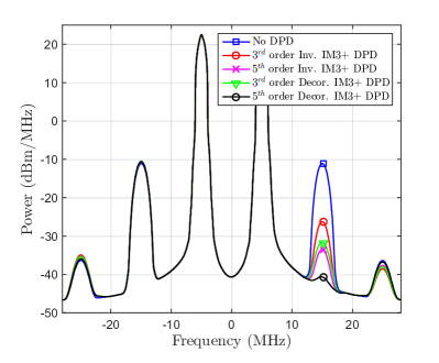
Figure 6: Baseband equivalent PA output spectrum at +23 dBm with two 1 MHz LTE-A UL carriers and 10 MHz CC separation using a fifth-order memoryless PA. $P^{th}$-order inverse and decorrelation-based IM3+ sub-band DPD solutions are compared, with both third-order and fifth-order nonlinear processing.

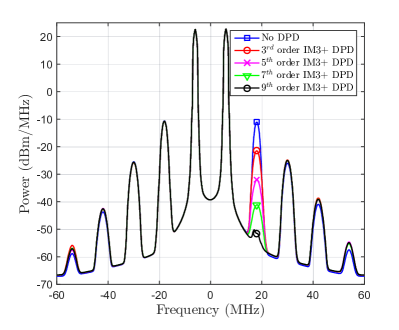
Figure 7: Baseband equivalent PA output spectrum at +24 dBm with two 1 MHz LTE-A UL carriers and 12 MHz CC separation using a ninth-order PA with memory. Different orders of the IM3+ sub-band DPD are compared, with memory depth equal to 1 per DPD SNL basis function.

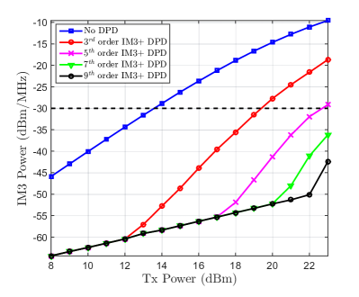
Figure 8: IM3 spurious emissions vs. TX power using different orders of the IM3+ sub-band DPD processing, with memory depth equal to 1 per DPD SNL basis function. A ninth-order PA with memory is used, and 2 dB Tx filter insertion loss is assumed.

V-C Performance of Proposed Higher-Order Sub-band DPD at IM3, IM5 and IM7

In this subsection, we evaluate the performance of the proposed sub-band DPD in the more realistic case of having memory in the PA. The PA model is a 9th-order parallel Hammerstein model, with four memory taps per branch, and the parameters have been identified using measurements with a true mobile PA transmitting at +24 dBm. The sub-band DPD structure contains now also memory, with two taps ($N=1$) per basis function. Block-adaptive learning principle is adopted, with 200 blocks each containing 1000 samples. The transmit waveform is otherwise identical to earlier cases, but the CC separation is now 12 MHz.

TABLE III: Comparison of quantitative running complexity and linearization performance of full-band versus sub-band DPD. Two 1 MHz LTE-A UL carriers with QPSK data modulation and 20 MHz carrier spacing are used.

	DPD Running Complexity			Transmitter Performance
	Coeffs	Fs [MSPS]	GFLOPS	EVM [%]	Positive IM3R [dBc]	Positive IM5R [dBc]	Output Power [dBm]
No DPD	N/A	N/A	N/A	1.2527	35.5744	56.4272	+20
Full-Band ILA DPD	20	189	31.941	0.1058	61.9428	63.9842	+19
IM3+ Sub-Band DPD	8	9	0.891	1.2489	68.3291	N/A	+20
IM5+ Sub-Band DPD	6	9	0.774	1.2529	N/A	71.9823	+20

Fig. 7 shows the effectiveness of the proposed higher-order sub-band DPDs, here processing the IM3+ sub-band, compared to the basic third-order solution presented earlier in [20]. Up to 40 dB suppression for the IM3 spurious emissions is shown when adopting ninth-order processing, something that has not been reported before in any prior works using a practical PA model with memory effects. Fig. 8 shows then how the IM3 spurious emission level changes with varying the TX power and using different sub-band DPD orders. The IM3 spurious emissions are clearly below the general spurious emission limit (-30 dBm/MHz) even at very high TX powers up to +23 dBm, when using a seventh-order, or higher, sub-band DPD.

Another main contribution in this paper is the extension of the IM3 sub-band DPD solution to include also higher-order IM sub-bands. Fig. 9 shows the performance of the negative IM5 and IM7 sub-band DPDs, in addition to the negative IM3 sub-band DPD, when ninth-order nonlinear processing is adopted in the sub-band DPDs. Up to 40 dB, 35 dB, and 18 dB of suppression is achieved at the negative IM3, IM5, and IM7 sub-bands, respectively. This shows the effectiveness of the proposed solutions in processing and suppressing also the spurious emissions at higher IM sub-bands.

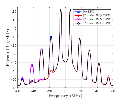
Figure 9: Baseband equivalent of two 1 MHz LTE-A UL carriers with 12 MHz separation using a ninth order PH PA extracted from a real mobile PA at +24 dBm. Ninth order negative IM3, IM5, and IM7 sub-band DPD solutions are shown, with memory depth equal to 1 per DPD SNL basis function.

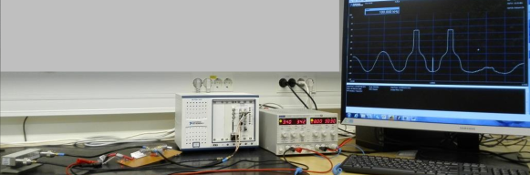
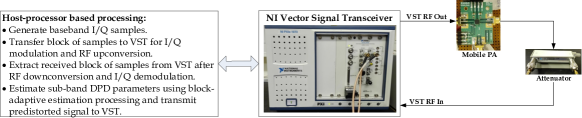
Figure 10: Hardware setup used in the RF measurements for testing and evaluating the proposed sub-band DPD.

V-D Full-Band versus Sub-band DPD Complexity and Performance Analysis

In this subsection, we compare the performance of our proposed sub-band DPD technique against that of a classical full-band DPD adopting parallel Hammerstein based wideband linearization and indirect learning architecture (ILA). The evaluation considers the linearization performance, complexity, and transmitter efficiency utilizing our earlier complexity analysis results reported in Section IV. The ninth-order full-band PH ILA DPD uses 100k samples for parameter learning, per ILA iteration, with a total of 2 ILA iterations, and the number of memory taps per PH branch is 4. The ninth-order block-adpative sub-band DPD, in turn, uses also a total of 200k samples with block size $M=1000$, and adopts two memory taps per DPD SNL basis function.

The results are collected in Table III, which shows that in addition to the significantly lower complexity measured by the number of GFLOPS, the sub-band DPD achieves better linearization performance in terms of spurious IMD suppression at the considered IM3 and IM5 sub-bands. On the other hand, the full-band DPD outperforms the sub-band DPD in terms of the inband distortion mitigation (i.e., EVM). This is expected, since the full-band DPD linearizes the whole transmit band, including the main CCs and the IMD spurious emissions. However, the EVM with the sub-band DPD is only around $1.25\%$ which is by far sufficient for modulations at least up to $64$-QAM. Additionally, the full-band DPD based on the ILA structure requires an additional 1 to 2 dB back off to guarantee stable operation, which is not required in the sub-band DPD. Thus the transmitter becomes more power efficient when using the sub-band DPD as shown in Table III. For fairness, it is to be acknowledged that a full-band DPD can typically enhance the EVM and ACLR, while the sub-band DPD concept is specifically targeting only the spurious emissions.

VI RF Measurement Results

In order to further demonstrate the operation of the proposed sub-band DPD solution, we next report results of comprehensive RF measurements using a commercial LTE-Advanced mobile terminal PA together with a vector signal transceiver (VST), which is implementing the RF modulation and demodulation. The actual sub-band DPD processing and parameter learning algorithms are running on a host processor.

The ACPM-5002-TR1 mobile power amplifier used in our measurements is designed for LTE-A UL band 25 (1850-1915 MHz), with 29 dB gain. The National Instruments (NI) PXIe-5645R VST includes both a vector signal generator (VSG), and a vector signal analyzer (VSA) with 80 MHz instantaneous bandwidth. In these experiments, the digital baseband waveform is divided into 50 blocks of size $M=10k$ samples which are first generated locally on the host processor, and then transferred to the VSG to perform RF I/Q modulation at the desired power level at the PA input. The VST RF output is then connected to the input port of the external power amplifier, whose output port is connected to the VST RF input through a 40 dB attenuator, implementing the observation receiver as illustrated also in Fig. 10. The VSA performs RF I/Q demodulation to bring the signal back to baseband. The baseband I/Q observation block is then filtered to select the IM3 sub-band which is used for block-based sub-band DPD learning, after proper alignment with the locally generated basis functions, as explained in Section III-C. The sub-band DPD block size $M$ used in these experiments is $10k$, and the DPD memory depth $N$ is $1$.

In general, two different intra-band LTE-A CA RF measurement examples are demonstrated in this subsection. The first experiment demonstrates the violation of the spurious emission limit due to the inband emission of the IM3+ spur, thus not being attenuated by the TX filter. The second experiment demonstrates an own RX desensitization example, in FDD transceiver context, where the IM3+ spur is located at the own RX band (1930-1995 MHz) and is not sufficiently attenuated by the duplexer TX filter. Notice that in principle, when tackling specifically the own RX desensitization problem with the proposed sub-band DPD solution, the main receiver of the FDD device could potentially be used as the observation receiver (i.e., learning the sub-band DPD coefficients without an extra auxiliary/observation receiver). However, such an approach would indeed be applicable only in the own RX desensitization case, while when mitigating other harmful emissions, an auxiliary observation receiver would anyway have to be adopted. Thus, in these RF measurements, we adopt the auxiliary receiver based approach, while consider further developments of the main receiver based parameter learning as an important topic for our future work.

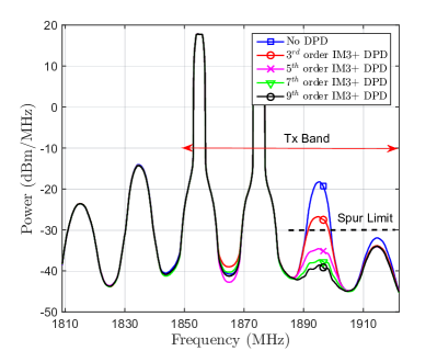
Figure 11: An LTE-A band 25 RF measurement example at the UE PA output showing the gain from using an IM3+ sub-band DPD. IM3 spur reduction with third, fifth, seventh, and ninth-order sub-band DPDs are demonstrated, using a real commercial mobile PA operating at +25 dBm. An LTE-A UL CA signal with two 3 MHz CCs and 20 MHz carrier spacing is used.

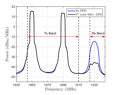
Figure 12: An LTE-A band 25 RF measurement example at the UE PA output showing the gain from using a ninth-order IM3+ sub-band DPD when the IM3+ is falling at own RX band. An LTE-A UL CA signal with two 5 MHz CCs and 40 MHz carrier spacing is used with a real commercial mobile PA operating at +25 dBm.

VI-A Spurious Emission Limit Violation

Fig. 11 shows the measured power spectral density at the PA output using the IM3 sub-band DPD with different orders. The adopted waveform is an intra-band CA LTE-A UL signal with 3 MHz per CC and 20 MHz carrier spacing. The power level at the PA output in this example is +25 dBm. The intermodulation distortion at the IM3+ sub-band is emitted inband, since the total TX band covers 1850-1915 MHz, and is clearly violating the spurious emission limit (-30 dBm/MHz) when no DPD is used. When using the sub-band DPD, the spurious emission level is well below the emission limit, given that at least 5th-order processing is deployed. In general, more than 20 dB of measured spurious emission suppression is achieved with the ninth order IM3 sub-band DPD, thus giving more than 10 dB additional gain compared to the basic third-order sub-band DPD as shown in Fig. 11. Notice that there is no need for predistorting the IM3- sub-band in this example, since those emissions will be filtered out by the TX filter.

VI-B Own Receiver Desensitization

Fig. 12 illustrates another LTE-A intra-band CA UL band 25 example, now with 5 MHz CC bandwidths and 40 MHz carrier spacing. The duplexing distance at LTE-A band 25 is only 80 MHz, thus the IM3+ spur at 1935 MHz in this example is falling on the own RX band, and therefore potentially desensitizing the own receiver. The power level at the PA output in this example is +25 dBm.

Then, by adopting a ninth-order IM3+ sub-band DPD, more than 20 dB of spurious emission suppression is achieved, as can be seen in Fig. 12. Again, two taps ($N=1$) per basis function are used, and block-adaptive parameter learning is deployed. Fig. 13 shows the real-time convergence of the sub-band DPD coefficients for the third, fifth, seventh, and ninth-order basis functions, respectively. It can be seen that the coefficients converge in a stable manner in a real RF environment due to the orthogonalization of the SNL basis functions, as explained in Section III-B.

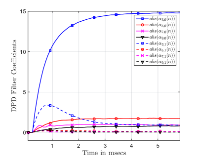
Figure 13: Convergence of the ninth-order sub-band DPD coefficients, with memory depth $N=1$ per basis function, when the positive IM3 sub-band is considered and block-adaptive learning is deployed. An RF measurement example with two 5 MHz LTE-A UL CCs and 40 MHz carrier spacing is used with a real commercial mobile PA operating at +25 dBm.

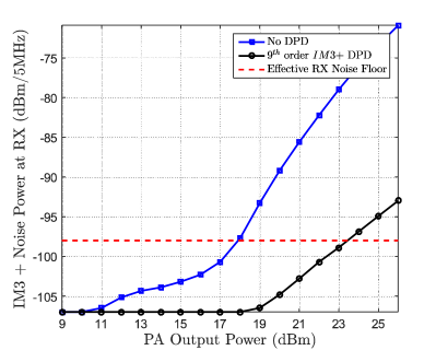
Figure 14: Integrated IM3+ sub-band power at own RX LNA input over 5 MHz vs. PA output power using ninth order IM3+ sub-band DPD processing, with memory depth equal to 1 per DPD SNL basis function. A commercial mobile PA operating at LTE band 25 is used in the RF measurements, and 65 dB duplexer TX filter attenuation [Avago_Duplexer] is assumed at the RX band.

In general, assuming a UE duplexer TX filter with 65 dB attenuation at the own RX band (e.g., ACMD-6125 Band 25 LTE-A UE Duplexer), the integrated power of the IM3+ spur at the RX band without DPD will be approximately -73 dBm/5MHz. This is 25 dB above the effective RX noise floor when assuming 9 dB UE RX noise figure (NF) [28]. This would thus cause significant own receiver desensitization that could lead to a complete blocking of the desired RX signal. On the other hand, when the proposed IM3+ sub-band DPD is deployed, the integrated power of the IM3+ spur at the RX band will be approximately -95 dBm/5MHz, which is only 3 dB above the effective RX noise floor, as shown also in Fig. 14. Though the residual spur is still slightly above the effective RX noise floor, the sensitivity degradation is substantially relaxed, despite operating at a maximum PA output power of +25 dBm. We elaborate on this further in Fig. 14, showing the integrated power of the IM3+ spur at the RX LNA input while changing the PA output power level. With a ninth order sub-band DPD, we can transmit up to +18 dBm PA output power with an effectively perfectly linear TX, in terms of IM3+ spur level, compared to +10 dBm PA output power without DPD. Additionally, with DPD, the integrated IM3+ power is less than the effective RX noise floor up to +23 dBm PA output power, while without DPD it is already 20 dB above the noise floor at the same power level.

VII Conclusions

In this article, a novel low-complexity sub-band digital predistortion (DPD) solution was proposed for suppressing unwanted spurious emissions in non-contiguous spectrum access. Novel decorrelation based adaptive parameter learning methods were also formulated, allowing efficient estimation and tracking with low computational complexity. All algorithm derivations and modeling were carried out in the general case of having memory in the PA as well as in the sub-band DPD processing. Different nonlinear distortion and processing orders, beyond classical third-order cases, were also reported. The proposed technique can find application in suppressing inband spurs which would violate the spurious emission limit, suppressing out-of-band spurs falling, e.g., on the own receiver band, or in protecting primary user transmissions in cognitive radio systems. A quantitative complexity analysis was presented, comparing the proposed solution to conventional full-band DPD solutions available in the literature. The performance was evaluated in a comprehensive manner, showing excellent linearization performance despite the considerably reduced complexity compared to classical full-band solutions. Finally, extensive RF measurement results using a commercial LTE-Advanced mobile power amplifier were reported, evidencing up to 22 dB suppression of the most problematic third-order spurious emissions.

Appendix A: Analytical MMSE Solution for Third-Order IM3 Sub-band DPD

Here, we derive the analytical minimum mean-square error solution shown in (32), which is used as a reference solution in simulations in Section V-A. We first define the so-called error signal as $e(n)=\tilde{y}_{IM3_{+}}(n)$, since with ideal predistortion the IM3+ sub-band signal would be zero, and thus the optimization means minimizing the power of this error signal. From (30), the error signal reads

$$e(n) =(f_{3}+f_{1}\alpha)u(n)+2f_{3}\alpha(|x_{1}(n)|^{2}+|x_{2}(n)|^{2})u(n)$$

$$+f_{3}|\alpha|^{2}\alpha|x_{1}(n)|^{4}|x_{2}(n)|^{2}u(n),$$ (66)

where $f_{1}$ and $f_{3}$ are the third-order memoryless PA model parameters, $\alpha$ denotes the DPD coefficient to be optimized, and $x_{1}(n)$ and $x_{2}(n)$ are the baseband equivalents of the two component carriers. The statistical expectation ${\rm I\kern-3.00003ptE}[|e(n)|^{2}]={\rm I\kern-3.00003ptE}[e(n)e^{*}(n)]$, assuming that the component carrier signals $x_{1}(n)$ and $x_{2}(n)$ are statistically independent, and ignoring some high-order vanishingly small terms, then reads

$${\rm I\kern-2.70003ptE}[e(n)e^{*}(n)]={\rm I\kern-2.70003ptE}_{42}\left[|f_{3}|^{2}+|f_{1}|^{2}|\alpha|^{2}+\alpha f_{1}f_{3}^{*}+\alpha^{*}f_{1}^{*}f_{3}\right]$$

$$+(2{\rm I\kern-2.70003ptE}_{62}+2{\rm I\kern-2.70003ptE}_{44})\left[|f_{3}|^{2}(\alpha+\alpha^{*})+|\alpha|^{2}(f_{1}f_{3}^{*}+f_{1}^{*}f_{3})\right]$$

$$+(4{\rm I\kern-2.70003ptE}_{46}+8{\rm I\kern-2.70003ptE}_{64}+4{\rm I\kern-2.70003ptE}_{82})|f_{3}|^{2}|\alpha|^{2},$$ (67)

where ${\rm I\kern-3.00003ptE}_{ij}$ is used as a shorthand notation for ${\rm I\kern-3.00003ptE}[|x_{1}|^{i}]{\rm I\kern-3.00003ptE}[|x_{2}|^{j}]$. Now, differentiating (67) with respect to $\alpha$, yields

$$\frac{\partial}{\partial\alpha}{\rm I\kern-2.70003ptE}[e(n)e^{*}(n)] ={\rm I\kern-2.70003ptE}_{42}\left[\alpha^{*}|f_{1}|^{2}+f_{1}f_{3}^{*}\right]$$

$$+(2{\rm I\kern-2.70003ptE}_{62}+2{\rm I\kern-2.70003ptE}_{44})\left[|f_{3}|^{2}+\alpha^{*}(f_{1}f_{3}^{*}+f_{1}^{*}f_{3})\right]$$

$$+(4{\rm I\kern-2.70003ptE}_{46}+8{\rm I\kern-2.70003ptE}_{64}+4{\rm I\kern-2.70003ptE}_{82})|f_{3}|^{2}\alpha^{*}.$$ (68)

Then, setting (68) to zero and solving for $\alpha$ yields the optimal MMSE DPD parameter, given by

$$\alpha_{MMSE}=$$

$$\dfrac{-\left[f_{1}f_{3}^{*}{\rm I\kern-2.70003ptE}_{42}+2|f_{3}|^{2}({\rm I\kern-2.70003ptE}_{62}+{\rm I\kern-2.70003ptE}_{44})\right]^{*}}{\left[|f_{1}|^{2}{\rm I\kern-2.70003ptE}_{42}+4\mathbb{R}(f_{1}f_{3}^{*})({\rm I\kern-2.70003ptE}_{62}+{\rm I\kern-2.70003ptE}_{44})+4|f_{3}|^{2}({\rm I\kern-2.70003ptE}_{46}+2{\rm I\kern-2.70003ptE}_{64}+{\rm I\kern-2.70003ptE}_{82})\right]^{*}},$$ (69)

where $\mathbb{R}(.)$ denotes the real-part operator. This concludes the proof.

Appendix B: Analytical Fifth-Order Inverse Based IM3 Sub-band DPD Solution

Here, we derive the $5^{th}$ order inverse solution for the IM3+ sub-band DPD, to be used as a reference solution in the simulations in Section V-B. The output of a memoryless $5^{th}$ order polynomial PA model is

$$y(n) =f_{1}x(n)+f_{3}|x(n)|^{2}x(n)+f_{5}|x(n)|^{4}x(n),$$ (70)

where $f_{1}$, $f_{3}$ and $f_{5}$ are the polynomial coefficients, and $x(n)$ is the composite baseband equivalent input signal, as given in (1). Through direct substitution of (1) in (70), the baseband equivalent IM3+ distortion term, located at three times the IF frequency, can be extracted and reads

$$y_{IM3_{+}}(n) =f_{3}(x_{2}^{*}(n)x_{1}^{2}(n))$$

$$+2f_{5}|x_{1}(n)|^{2}(x_{2}^{*}(n)x_{1}^{2}(n))$$

$$+3f_{5}|x_{2}(n)|^{2}(x_{2}^{*}(n)x_{1}^{2}(n)).$$ (71)

Stemming from the signal structure in (71), the sub-band DPD injection signal is composed of three basis functions of the form $x_{2}^{*}(n)x_{1}^{2}(n)$, $|x_{1}(n)|^{2}x_{2}^{*}(n)x_{1}^{2}(n)$ and $|x_{2}(n)|^{2}x_{2}^{*}(n)x_{1}^{2}(n)$. In case of fifth-order inverse based sub-band DPD, these basis functions are multiplied by proper coefficients such that all the distortion terms at the IM3+ sub-band at the PA output, up to order five, are cancelled. Thus, incorporating such DPD processing, yet with arbitrary coefficients, the composite baseband equivalent PA input signal reads

$$\begin{split}\tilde{x}(n)&=x_{1}(n)e^{j2\pi\frac{f_{IF}}{f_{s}}n}+x_{2}(n)e^{-j2\pi\frac{f_{IF}}{f_{s}}n}\\ &+\alpha_{3,inv}(x_{2}^{*}(n)x_{1}^{2}(n))e^{j2\pi\frac{3f_{IF}}{f_{s}}n}\\ &+\alpha_{51,inv}|x_{1}(n)|^{2}(x_{2}^{*}(n)x_{1}^{2}(n))e^{j2\pi\frac{3f_{IF}}{f_{s}}n}\\ &+\alpha_{52,inv}|x_{2}(n)|^{2}(x_{2}^{*}(n)x_{1}^{2}(n))e^{j2\pi\frac{3f_{IF}}{f_{s}}n},\end{split}$$ (72)

where the subscript $inv$ in the coefficients is emphasizing the $P^{th}$-order inverse based solution. Substituting (72) in (70), and extracting the third and fifth order IM3+ terms, yields

$$\begin{split}\tilde{y}&{}_{IM3_{+}}(n)=(f_{1}\alpha_{3,inv}+f_{3})x_{2}^{*}(n)x_{1}^{2}(n)\\ &+(f_{1}\alpha_{51,inv}+2f_{3}\alpha_{3,inv}+2f_{5})|x_{1}(n)|^{2}(x_{2}^{*}(n)x_{1}^{2}(n))\\ &+(f_{1}\alpha_{52,inv}+2f_{3}\alpha_{3,inv}+3f_{5})|x_{2}(n)|^{2}(x_{2}^{*}(n)x_{1}^{2}(n)).\end{split}$$ (73)

From (73), we now can easily obtain the fifth-order inverse coefficients that null the third and fifth-order terms, yielding

$$\begin{split}\alpha_{3,inv}&=-\frac{f_{3}}{f_{1}},\\ \alpha_{51,inv}=2\frac{f_{3}^{2}}{f_{1}^{2}}-2\frac{f_{5}}{f_{1}},\>&\>\alpha_{52,inv}=2\frac{f_{3}^{2}}{f_{1}^{2}}-3\frac{f_{5}}{f_{1}}.\end{split}$$

This concludes the derivation.

Mahmoud Abdelaziz (S’13) received the B.Sc. degree (with honors) and M.Sc. degree in Electronics and Electrical Communications Engineering from Cairo University, Egypt, in 2006 and 2011. He is currently pursuing the Doctoral degree at Tampere University of Technology, Finland where he works as a researcher with the Department of Electronics and Communications. From 2007 to 2012 he has been working as a communication systems and signal processing engineer at Newport Media, as well as other companies in the wireless industry. His research interests include statistical and adaptive signal processing in flexible radio transceivers, wideband digital pre-distortion, and cognitive radio systems.

Lauri Anttila (S’06, M’11) received the M.Sc. degree and D.Sc. (Tech) degree (with honors) in electrical engineering from Tampere University of Technology (TUT), Tampere, Finland, in 2004 and 2011. Currently, he is a Senior Research Fellow at the Department of Electronics and Communications Engineering at TUT. His research interests are in signal processing for wireless communications, in particular radio implementation challenges in 5G cellular radio and full-duplex radio, flexible duplexing techniques, and transmitter and receiver linearization. He has co-authored over 60 peer reviewed articles in these areas, as well as two book chapters.

Chance Tarver received a B.S. degree in electrical engineering from Louisiana Tech University, Ruston, LA, in 2014, and his M.S. degree in electrical and computer engineering in 2016 from Rice University, Houston, TX. He is currently a Ph.D. student in the Department of Electrical and Computer Engineering at Rice University. His research interests include software defined radio and signal processing for wireless communications.

Kaipeng Li (S’14) received his B.S. degree in physics from Nanjing University, Nanjing, China, in 2013, and his M.S. degree in electrical and computer engineering from Rice University in 2015. He is currently a Ph.D. candidate in the Department of Electrical and Computer Engineering at Rice University, Houston, Texas. His research interests include digital signal processing, parallel computing on GPGPU and multicore CPU, software-defined radios and massive MIMO systems.

Joseph R. Cavallaro (S’78, M’82, SM’05, F’15) received the B.S. degree from the University of Pennsylvania, Philadelphia, PA, in 1981, the M.S. degree from Princeton University, Princeton, NJ, in 1982, and the Ph.D. degree from Cornell University, Ithaca, NY, in 1988, all in electrical engineering. From 1981 to 1983, he was with AT$\&$T Bell Laboratories, Holmdel, NJ. In 1988, he joined the faculty of Rice University, Houston, TX, where he is currently a Professor of electrical and computer engineering. His research interests include computer arithmetic, and DSP, GPU, FPGA, and VLSI architectures for applications in wireless communications. During the 1996-1997 academic year, he served at the National Science Foundation as Director of the Prototyping Tools and Methodology Program. He was a Nokia Foundation Fellow and a Visiting Professor at the University of Oulu, Finland in 2005 and continues his affiliation there as an Adjunct Professor. He is currently the Director of the Center for Multimedia Communication at Rice University. He is a Fellow of the IEEE and a Member of the IEEE SPS TC on Design and Implementation of Signal Processing Systems and the Chair-Elect of the IEEE CAS TC on Circuits and Systems for Communications. He is currently an Associate Editor of the IEEE Transactions on Signal Processing, the IEEE Signal Processing Letters, and the Journal of Signal Processing Systems. He was Co-chair of the 2004 Signal Processing for Communications Symposium at the IEEE Global Communications Conference and General/Program Co-chair of the 2003, 2004, and 2011 IEEE International Conference on Application-Specific Systems, Architectures and Processors (ASAP), General/Program Co-chair for the 2012, 2014 ACM/IEEE GLSVLSI, Finance Chair for the 2013 IEEE GlobalSIP conference, and TPC Co-Chair of the 2016 IEEE SiPS workshop. He was a member of the IEEE CAS Society Board of Governors during 2014.

Mikko Valkama (S’00, M’01, SM’15) was born in Pirkkala, Finland, on November 27, 1975. He received the M.Sc. and Ph.D. Degrees (both with honors) in electrical engineering (EE) from Tampere University of Technology (TUT), Finland, in 2000 and 2001, respectively. In 2002, he received the Best Ph.D. Thesis -award by the Finnish Academy of Science and Letters for his dissertation entitled ”Advanced I/Q signal processing for wideband receivers: Models and algorithms”. In 2003, he was working as a visiting researcher with the Communications Systems and Signal Processing Institute at SDSU, San Diego, CA. Currently, he is a Full Professor and Department Vice-Head at the Department of Electronics and Communications Engineering at TUT, Finland. His general research interests include communications signal processing, estimation and detection techniques, signal processing algorithms for software defined flexible radios, cognitive radio, full-duplex radio, radio localization, 5G mobile cellular radio, digital transmission techniques such as different variants of multicarrier modulation methods and OFDM, and radio resource management for ad-hoc and mobile networks.

References

- [1] S. Parkvall, A. Furuskar, and E. Dahlman, “Evolution of LTE toward IMT-advanced,” IEEE Commun. Mag., vol. 49, no. 2, pp. 84–91, February 2011.
- [2] LTE Evolved Universal Terrestrial Radio Access (E-UTRA) User Equipment (UE) radio transmission and reception, 3GPP TS 36.101 V12.4.0 (Release 12), June 2014.
- [3] S.A. Bassam, W. Chen, M. Helaoui, and F.M. Ghannouchi, “Transmitter architecture for CA: Carrier Aggregation in LTE-Advanced systems,” IEEE Microw. Mag., vol. 14, no. 5, pp. 78–86, July 2013.
- [4] C. Park, L. Sundström, A. Wallen, and A. Khayrallah, “Carrier aggregation for LTE-advanced: Design challenges of terminals,” IEEE Commun. Mag., vol. 51, no. 12, pp. 76–84, Dec. 2013.
- [5] R4-121205, “Way forward for non-contiguous intraband transmitter aspects.”, 3GPP Tech. Rep., Feb. 2013.
- [6] R4-124353, “Non-contiguous intraband unwanted emission.”, 3GPP Tech. Rep., Feb. 2013.
- [7] H. Gandhi, D. Greenstreet, and J. Quintal, “Digital Radio Front-End strategies provide game-changing benefits for small cell base stations,” Tech. Rep., Texas Instruments, May 2013.
- [8] L. Guan and A. Zhu, “Green communications: Digital predistortion for wideband RF power amplifiers,” IEEE Microw. Mag., vol. 15, no. 7, pp. 84–89, Dec. 2014.
- [9] R4-123797, “UE reference sensitivity requirements with two UL carriers.,” 3GPP Tech. Rep., Feb. 2013.
- [10] International Telecommunication Union Radio Communication Sector, Recommendation ITU-R SM.329-12 Unwanted emissions in the spurious domain..
- [11] Chao Yu, Wenhui Cao, Yan Guo, and A. Zhu, “Digital Compensation for Transmitter Leakage in Non-Contiguous Carrier Aggregation Applications With FPGA Implementation,” IEEE Trans. Microw. Theory Techn., vol. 63, no. 12, pp. 4306–4318, Dec 2015.
- [12] A. Kiayani, M. Abdelaziz, L. Anttila, V. Lehtinen, and M. Valkama, “Digital Mitigation of Transmitter-Induced Receiver Desensitization in Carrier Aggregation FDD Transceivers,” IEEE Trans. Microw. Theory Techn., vol. 63, no. 11, pp. 3608–3623, Nov 2015.
- [13] S.A. Bassam, F.M. Ghannouchi, and M. Helaoui, “2-D Digital Predistortion (2-D-DPD) architecture for concurrent dual-band transmitters,” IEEE Trans. Microw. Theory Techn., vol. 59, no. 10, pp. 2547–2553, Oct. 2011.
- [14] P. Roblin, C. Quindroit, N. Naraharisetti, S. Gheitanchi, and M. Fitton, “Concurrent linearization,” IEEE Microw. Mag., vol. 14, no. 7, pp. 75–91, Nov. 2013.
- [15] Y. Liu, J. Yan, and P. Asbeck, “Concurrent dual-band digital predistortion with a single feedback loop,” IEEE Trans. Microw. Theory Techn., vol. 63, no. 5, pp. 1556–1568, May 2015.
- [16] P. Roblin, S. K. Myoung, D. Chaillot, Y. G. Kim, A. Fathimulla, J. Strahler, and S. Bibyk, “Frequency-selective predistortion linearization of RF power amplifiers,” IEEE Trans. Microw. Theory Techn., vol. 56, no. 1, pp. 65–76, Jan. 2008.
- [17] J. Kim, P. Roblin, D. Chaillot, and Z. Xie, “A generalized architecture for the frequency-selective digital predistortion linearization technique,” IEEE Trans. Microw. Theory Techn., vol. 61, no. 1, pp. 596–605, Jan. 2013.
- [18] S.A. Bassam, M. Helaoui, and F.M. Ghannouchi, “Channel-selective multi-cell digital predistorter for multi-carrier transmitters,” IEEE Trans. Microw. Theory Techn., vol. 60, no. 8, pp. 2344–2352, Aug. 2012.
- [19] M. Abdelaziz, L. Anttila, A. Mohammadi, F. Ghannouchi, and M. Valkama, “Reduced-complexity power amplifier linearization for carrier aggregation mobile transceivers,” in IEEE International Conference on Acoustics, Speech, and Signal Processing, pp. 3908–3912, May 2014.
- [20] M. Abdelaziz, L. Anttila, J.R. Cavallaro, S. Bhattacharyya, A. Mohammadi, F.M. Ghannouchi, M. Juntti, and M. Valkama, “Low-complexity digital predistortion for reducing power amplifier spurious emissions in spectrally-agile flexible radio,” in 9th International Conference on Cognitive Radio Oriented Wireless Networks, pp. 323–328, June 2014.
- [21] M. Abdelaziz, C. Tarver, K. Li, L. Anttila, R. Martinez, M. Valkama, J. R. Cavallaro, “Sub-band digital predistortion for noncontiguous transmissions: Algorithm development and real-time prototype implementation,” in 49th Asilomar Conference on Signals, Systems and Computers, pp. 1180–1186, Nov. 2015.
- [22] M. Abdelaziz, Z. Fu, L. Anttila, A. M. Wyglinski and M. Valkama, “Digital predistortion for mitigating spurious emissions in spectrally agile radios,” IEEE Commun. Mag., vol. 54, no. 3, pp. 60–69, March 2016.
- [23] Z. Fu, L. Anttila, M. Abdelaziz, M. Valkama, and A. M. Wyglinski, “Frequency-Selective Digital Predistortion for Unwanted Emission Reduction,” IEEE Trans. Commun., vol. 63, no. 1, pp. 254–267, Jan. 2015.
- [24] A.S. Tehrani, H. Cao, S. Afsardoost, T. Eriksson, M. Isaksson, and C. Fager, “A comparative analysis of the complexity/accuracy tradeoff in power amplifier behavioral models,” IEEE Trans. Microw. Theory Techn., vol. 58, no. 6, pp. 1510–1520, June 2010.
- [25] H. Qian, S. Yao, H. Huang, and W. Feng, “A low-complexity digital predistortion algorithm for power amplifier linearization,” IEEE Trans. Broadcast., vol. 60, no. 4, pp. 670–678, Dec. 2014.
- [26] W. Hoffmann, “Iterative algorithms for Gram Schmidt orthogonalization,” Computing, vol. 41, no. 4, pp. 335–348, 1989.
- [27] M. Saint-Laurent et al., “A 28 nm DSP powered by an on-chip LDO for high-performance and energy-efficient mobile applications,” IEEE J. Solid-State Circuits, vol. 50, no. 1, pp. 81–91, Jan 2015.
- [28] LTE Evolved Universal Terrestrial Radio Access (E-UTRA) RF system scenarios, 3GPP TR 36.942 V10.2.0 (Release 10), May 2011.